Insuring uninsurable income

Abstract

This paper presents a method to avoid the ominous prediction of the previous work: if insured incomes of infinitely lived individuals are unobservable, then efficient allocations lead to permanent welfare inequality between individuals and immiseration of society. The proposed mechanism (i) promises within-period full insurance by postponing risks ; (ii) it does not lead to social ranking among the same age groups; and (iii) it could be sustainable.

JEL: D61; D82.

1 Introduction

An infinite period contract between a firm and individuals whose income is private information is said to lead to an immiseration outcome: individuals’ utility from consumption converges to negative infinity and welfare inequality grows unboundedly [Green, 1987, Thomas and Worrall, 1990, Atkeson and Lucas, 1992, Phelan, 1998]. The existing literature concludes that in the absence of full information, efficient allocations are achieved only at the cost of permanent inequality [Atkeson and Lucas, 1992, Phelan, 2006] or individuals have preferences that almost do not discount future values [Carrasco et al., 2019].

This paper presents a broadly Pareto optimal mechanism that could be a solution to this impossibility problem. The proposed mechanism (i) provides within-period full insurance with inter-period risk transfer; (ii) it does not lead to social ranking among the same age groups; (iii) it could be sustainable. This inter-period risk transfer mechanism in (i) is adapted from Marcet and Marimon [1992].

In a normalised expression, the value of the individual utility of this within-period full insurance in (i) is equal to the value of the individual lifetime utility of this full insurance being guaranteed forever. However, this is a trade-off with inter-period risk transfers. This trade-off is acceptable if we value the equality of individuals and the sustainability of society, as partly mentioned in (ii) and (iii). As previous studies show, if we try to cover within-period risks with within-period income among individuals who privately know their own income, its efficiency is a trade-off with extreme permanent inequality and immiseration in society. The proposed mechanism could maintain equality of opportunity because individuals continue to take their own risks that were postponed in the previous period. However, it is not a version of autarky, since the postponed income shocks are realised biased towards higher incomes. This feature could reduce the contract value of the firm in the long run and could make the mechanism unworkable. However, if we can expect that a new set of individuals to join the mechanism in each period, then the mechanims could be sustainable.

The proposed mechanism is efficient in the sense that it achieves full information Pareto optimality if the degree of risk aversion of individuals is not too large relative to the range of their income shocks. Otherwise, it does not, because it is forced to temporarily change the optimal transfer rules when the contract value that the planner wants to promise cannot be translated into individual utilities. This restriction follows from the assumption that the individual utilities are bounded from above. This assumption is a sufficient condition to ensure that a sequence of individuals’ lifetime utilities converges to an integrable random variable, and does not preclude the possibility that it also converges with some unbounded utilities.

This paper is structured as follows. Section 2 introduces the model and proposes the mechanism using the inter-period risk transfers. Section 3 shows the properties of the proposed mechanism. Section 4 provides comparisons with previous work, and section 5 provides conclusions.

2 Model

Consider a planner, a risk-neutral firm and a continuum of infinitely lived risk-averse individuals on the unit interval. Let $(\Omega,\mathcal{F},P)$ be a probability space, and let $\{e_{t}\}_{t\in\mathbb{N}\cup\{0\}}$ be a sequence of integrable random variables on $(\Omega,\mathcal{F},P)$ denoting idiosyncratic income shocks in a sequence of periods. These income shocks take values in $E:=\{e^{1},e^{2},\dots,e^{M}\}$, where $e^{i}\in\mathbb{R}_{+}$ with $e^{i}<e^{j}$ for $i<j\in\{1,\dots,M\}$, $M\geq 5$. The planner considers a transfer mechanism $\Gamma$ that repeats from a given period to infinity, using a transfer function $\tau:\mathbb{R}_{+}\to\mathbb{R}$ and allocation weights $\lambda\in\mathbb{R}_{++}$.

2.1 Pareto optimal contracts with full information

Let us first consider the case of the full information case. Following Marcet and Marimon [1992], we assume that the planner considers an efficient transfer mechanism with some weight given to the risk-averse individuals. If the weight is $\lambda_{0}>0$ and the initial income of the representative individual is $e_{0}\in E$, the planner’s problem is written as

$$\max_{\tau} (1-\beta)\mathrm{E}_{0}[\sum_{t=0}^{\infty}\beta^{t}[\lambda_{0}u(c_{t})-\tau(e_{t})]],$$ (1)

where $\mathrm{E}_{0}$ is the conditional expectation given $e_{0}$, $u:\mathbb{R}_{+}\to\mathbb{R}$ is the individual’s utility function, $c_{t}=e_{t}+\tau(e_{t})$ is consumption in period $t$, and $\beta\in(0,1)$ is the common discount factor for the parties. The utility function $u$ is assumed to be $u^{\prime}>0$, $u^{\prime\prime}<0$, to satisfy the Inada conditions ($\lim_{c\to 0}u^{\prime}(c)=+\infty$, $\lim_{c\to\infty}u^{\prime}(c)=0$) and to be bounded from above. From the first order condition,

$$u^{\prime}(c_{t})=\frac{1}{\lambda_{0}}\text{ for }t\in\mathbb{N}\cup\{0\}$$

and we obtain $c_{t}=(u^{\prime})^{-1}(\lambda_{0}^{-1})$ for $t\in\mathbb{N}\cup\{0\}$. This is the Pareto optimal contract that gives the individual constant consumption in each period.

Let $v_{1}:\mathbb{R}_{++}\times\mathbb{R}_{+}\to\mathbb{R}$ and $v_{2}:\mathbb{R}_{++}\times\mathbb{R}_{+}\to\mathbb{R}$ be the contract values of individuals and the firm respectively. Then, for given $\lambda_{0}>0$ and $e_{0}\in E$, these contract values are written as follows.

$$v_{1}(\lambda_{0},e_{0}) :=(1-\beta)\mathrm{E}_{0}[\sum_{t=0}^{\infty}\beta^{t}u(c_{t})]=u((u^{\prime})^{-1}(\lambda_{0}^{-1}))=:\overline{v}_{1}(\lambda_{0})$$

$$v_{2}(\lambda_{0},e_{0}) :=(1-\beta)\mathrm{E}_{0}[\sum_{t=0}^{\infty}\beta^{t}(-\tau(e_{t}))],$$

$$\overline{v}_{2}(\lambda_{0}) :=\mathrm{E}[v_{2}(\lambda_{0},e_{t})].$$

Note that the individual contract values could be seen as a function of the initial allocation weight $\lambda_{0}$. So we write it $\overline{v}_{1}(\lambda_{0})$. On the other hand, the firm’s contract value still depends on incomes. We write its expectation $\overline{v}_{2}(\lambda_{0})$. We also let $\tau^{*}(\cdot\ |\lambda):\mathbb{R}_{+}\to\mathbb{R}$ be the solution of the problem (1) for given $\lambda\in\mathbb{R}_{++}$: for $x\in\mathbb{R}_{+}$

$$\tau^{*}(x|\lambda):=(u^{\prime})^{-1}(\lambda^{-1})-x.$$

We will use these notations in the following section for the case where income is private information.

2.2 Pareto optimal contracts with asymmetric information

If income is private information, the planner must ask individuals to report their income. Since this is known to lead to an immiseration outcome, the planner does not hope to manipulate the transfer function $\tau^{*}$ to provide incentives for truth telling. The planner takes an alternative approach. It is to vary the allocation weight $\lambda$ in each period. This could also be an incentive to tell the truth as follows. Suppose that for a given allocation weight $\lambda$ for a period, the planner promises to secure the expected utility $\overline{v}_{1}(\lambda)$ for the period, and the allocation weight for the next period is renewed taking into account the current allocation weight and the reported income in the current period. If an individual truthfully reports income $e$ in a period $t$, then the lifetime utility is

$$\overline{v}_{1}(\lambda)=\mathrm{E}\big{[}(1-\beta)u(e+\tau^{*}(e|\lambda))+\beta\overline{v}_{1}(\lambda^{\prime}(e|\lambda))\big{]},$$ (2)

where $\lambda^{\prime}(\cdot|\lambda):E\to\mathbb{R}_{++}$ is the allocation weight for the next period as determined by the self-report. Truth telling is then induced if, given the current allocation weight $\lambda$, the renewed allocation weight $\lambda^{\prime}$ satisfies the following incentive constraints.

$$(1-\beta)u(e+\tau^{*}(e|\lambda)) +\beta\overline{v}_{1}(\lambda^{\prime}(e|\lambda))$$

$$\geq(1-\beta)u(e+\tau^{*}(\tilde{e}|\lambda))+\beta\overline{v}_{1}(\lambda^{\prime}(\tilde{e}|\lambda))\text{ for }e,\tilde{e}\in E.$$ (3)

Such an allocation weight $\lambda^{\prime}$ that satisfies both (2) and (3) could be adapted from the $\lambda$ mechanism of Marcet and Marimon [1992], provided that the mechanism provides $\lambda^{\prime}$ that ensures that the level of expected utility for the next period does not exceed the supremum of the individual’s utility function. That is, let $S$ be the supremum of the individual’s utility function, $S=\sup_{x\in\mathbb{R}_{+}}u(x)$. For given $\lambda>0$, if $\overline{v}_{1}(\lambda)+\lambda^{-1}\beta^{-1}(v_{2}(\lambda,e)-\overline{v}_{2}(\lambda))<S$ for all $e\in E$, define $\lambda^{\prime}$ such that

$$\lambda^{\prime}(e|\lambda)=\overline{v}_{1}^{-1}\big{(}\overline{v}_{1}(\lambda)+\lambda^{-1}\beta^{-1}(v_{2}(\lambda,e)-\overline{v}_{2}(\lambda))\big{)}.$$ (4)

Note that $u(e+\tau^{*}(e|\lambda))=u((u^{\prime})^{-1}(\lambda^{-1}))=\overline{v}_{1}(\lambda)$. So the lifetime utility with $\lambda^{\prime}$ defined in (4) satisfies (2):

$$\mathrm{E}[(1-\beta)u(e+\tau^{*}(e|\lambda)) +\beta\overline{v}_{1}(\lambda^{\prime}(e|\lambda))]$$

$$=\mathrm{E}[\overline{v}_{1}(\lambda)+\lambda^{-1}(v_{2}(\lambda,e)-\overline{v}_{2}(\lambda))]=\overline{v}_{1}(\lambda).$$

In addition, since the planner’s objective function in the problem (1) if the weight $\lambda_{0}=\lambda$:

$$\lambda\big{[}(1-\beta)u(e+\tau^{*}(e|\lambda))+\beta\overline{v}_{1}(\lambda)\big{]}+v_{2}(\lambda,e)$$

is maximised at income $e$, the following inequality holds.

$$\lambda\big{[}(1-\beta) u(e+\tau^{*}(e|\lambda))+\beta\overline{v}_{1}(\lambda)\big{]}+v_{2}(\lambda,e)-\overline{v}_{2}(\lambda)$$

$$\geq\lambda[(1-\beta)u(e+\tau^{*}(\tilde{e}|\lambda))+\beta\overline{v}_{1}(\lambda)]+v_{2}(\lambda,\tilde{e})-\overline{v}_{2}(\lambda)\quad\text{ for }e,\tilde{e}\in E.$$

However, since the term on the left-hand side of the above inequality is equal to the weighted lifetime utility, we have the following inequality and see that (3) holds.

$$\lambda\big{[}(1-\beta)u(e+\tau^{*}(e|\lambda)) +\beta\overline{v}_{1}(\lambda)\big{]}+v_{2}(\lambda,e)-\overline{v}_{2}(\lambda)$$

$$=\lambda\big{[}(1-\beta)u(e+\tau^{*}(e|\lambda))+\beta\overline{v}_{1}(\lambda^{\prime}(e|\lambda))\big{]}$$

$$\geq\lambda[(1-\beta)u(e+\tau^{*}(\tilde{e}|\lambda))+\beta\overline{v}_{1}(\lambda)]+v_{2}(\lambda,\tilde{e})-\overline{v}_{2}(\lambda)$$

$$=\lambda\big{[}(1-\beta)u(e+\tau^{*}(\tilde{e}|\lambda))+\beta\overline{v}_{1}(\lambda^{\prime}(\tilde{e}|\lambda))\big{]}\quad\text{ for }e,\tilde{e}\in E.$$

This might give some intuition about the incentive mechanism. Since $v_{2}(\lambda,e)-\overline{v}_{2}(\lambda)=(1-\beta)(e-\mathrm{E}[e_{t}])$, if reported incomes $e\in E$ are above the average income, $\mathrm{E}[e_{t}]$, this will be rewarded with higher allocation weights for the next period. Conversely, if reported incomes $e\in E$ are below the average income, $\mathrm{E}[e_{t}]$, this will result in lower allocation weights for the next period.

On the other hand, if there is an income $\hat{e}\in E$ such that, for given $\lambda$, the mechanism provides $\lambda^{\prime}$ whose promised value of expected utility for the next period is above the supremum of the individual’s utility function, the planner must find the closest allocation weight to the income $\hat{e}$ for which there is a certainty equivalent to the amount the planner should promise for the next period. That is, for given $\lambda$, if there is $\hat{e}\in E$ such that $\overline{v}_{1}(\lambda)+\lambda^{-1}\beta^{-1}(v_{2}(\lambda,\hat{e})-\overline{v}_{2}(\lambda))\geq S$, for reported income $e\in E$, define $\lambda^{\prime}$ such that

$$\lambda^{\prime}(e|\lambda)=\overline{v}_{1}^{-1}\big{(}\overline{v}_{1}(\lambda)+\lambda^{-1}\beta^{-1}(v_{2}(\lambda,\min\{e,\overline{e}_{\lambda}\})-\mathrm{E}[v_{2}(\lambda,\min\{e_{t},\overline{e}_{\lambda}\})])\big{)},$$ (5)

where $\overline{e}_{\lambda}$ is defined such that

$$\overline{e}_{\lambda}=\arg\max_{e^{\prime}\in E_{N}}v_{2}(\lambda,e^{\prime})$$

subject to

$$\overline{v}_{1}(\lambda)+\frac{1}{\lambda\beta}\big{(}v_{2}(\lambda,e^{\prime})-\mathrm{E}[v_{2}(\lambda,\min\{e_{t},e^{\prime}\})]\big{)}<S,$$

where $E_{N}\supset E$ is a set with $|E_{N}|=N>M$, $N\in\mathbb{N}$, and for $e\in E_{N}$ $e^{1}\leq e\leq e^{M}$. This adjustment also changes the transfers in the current period $t$, and the recursive relation in (5) satisfies the following corresponding incentive constraint.

$$(1-\beta)u(e +\tau^{*}(\min\{e,\overline{e}_{\lambda}\}|\lambda))+\beta\overline{v}_{1}(\lambda^{\prime}(e|\lambda))$$

$$\geq(1-\beta)u(e+\tau^{*}(\min\{\tilde{e},\overline{e}_{\lambda}\}|\lambda))+\beta\overline{v}_{1}(\lambda^{\prime}(\tilde{e}|\lambda))\text{ for }e,\tilde{e}\in E.$$ (6)

This is because the transfer $\tau^{*}(\min\{e,\overline{e}_{\lambda}\}|\lambda)$ in (6) is the solution to the problem (1) subject to $\tau(e_{t})\geq(u^{\prime})^{-1}(\lambda^{-1})-\overline{e}_{\lambda}$ for $t\in\mathbb{N}\cup\{0\}$ when $\lambda_{0}=\lambda$. In other words, since the transfer to the firm is constant for individuals whose income is above the threshold $\overline{e}_{\lambda}$, they are indifferent between reporting and misreporting their true income.

With respect to the promise-keeping constraint, it holds because the expectation of the left-hand side of the inequality in (6) is greater than or equal to the promised level of lifetime utility $\overline{v}_{1}(\lambda)$:

$$\mathrm{E}\big{[}(1-\beta)u(e+\tau^{*}(\min(e,\overline{e}_{\lambda})|\lambda))+\beta\overline{v}_{1}(\lambda^{\prime})\big{]}\geq\overline{v}_{1}(\lambda).$$

An inter-period transfer mechanism $\Gamma^{i}$ is represented by a sequence of allocation weights $(\lambda_{t})_{t\in\mathbb{N}\cup\{0\}}$ satisfying $\overline{v}_{1}(\lambda_{0})\in[\lambda_{\text{min}},\lambda_{\text{max}}]$, either (4) or (5), and the corresponding transfers: $\tau^{*}(e_{t}|\lambda_{t})$ for $\lambda_{t}$ in (4) and $\tau^{*}(\min\{e_{t},\overline{e}_{\lambda_{t}}\}|\lambda_{t})$ for $\lambda_{t}$ in (5). The minimum value of the allocation weights $\lambda_{\text{min}}$ is set at the value of the allocation weight that provides the lifetime utility in the state of autarky. The maximum value of the allocation weights $\lambda_{\text{max}}$ is the value of the allocation weight that provides a fair gamble $\overline{v}_{1}(\lambda_{\text{max}})=u(\mathrm{E}[e_{t}])$.

One could see a case where an allocation weight $\lambda_{t}$ in $\Gamma^{i}$ satisfies (5), for example, if the individuals’ utilities have constant absolute risk aversion, and if it is greater than $\beta/((1-\beta)(e^{M}-\mathrm{E}[e_{t}]))$. To see this, let $F(\lambda)=\overline{v}_{1}(\lambda)+\lambda^{-1}\beta^{-1}(v_{2}(\lambda,e^{M})-\overline{v}_{2}(\lambda))$. If the Arrow-Pratt measure of absolute risk aversion at the optimal level of consumption is less than or equal to $\beta/((1-\beta)(e^{M}-\mathrm{E}[e_{t}]))$, then $F(\lambda)$ is increasing in $\lambda$:

$$F^{\prime}(\lambda)\geq 0\text{ if }-\frac{u^{\prime\prime}((u^{\prime})^{-1}(\lambda^{-1}))}{u^{\prime}((u^{\prime})^{-1}(\lambda^{-1}))}\leq\frac{\beta}{(1-\beta)(e^{M}-\mathrm{E}[e_{t}])}.$$

If the Arrow-Pratt measure of absolute risk aversion at the optimal level of consumption is greater than $\beta/((1-\beta)(e^{M}-\mathrm{E}[e_{t}]))$, then $F(\lambda)$ is decreasing in $\lambda$:

$$F^{\prime}(\lambda)<0\text{ if }-\frac{u^{\prime\prime}((u^{\prime})^{-1}(\lambda^{-1}))}{u^{\prime}((u^{\prime})^{-1}(\lambda^{-1}))}>\frac{\beta}{(1-\beta)(e^{M}-\mathrm{E}[e_{t}])}.$$

In the latter case, if the absolute risk aversion is constant, since $\lim_{\lambda\to 0}F^{\prime}(\lambda)=-\infty$, there is a threshold $\overline{\lambda}$ below which $F(\lambda)\geq S$.

The inter-period transfer mechanism $\Gamma^{i}$ is sequentially incentive compatible. Furthermore, if $(\lambda_{t})$ continues to satisfy (4), like the $\lambda$ mechanism of Marcet and Marimon [1992], $\Gamma^{i}$ is sequentially efficient. That is, sequentially incentive compatible and not dominated by other sequentially incentive compatible mechanisms.

Proposition 2.1.

$\Gamma^{i}$ is sequentially incentive compatible. Furthermore, if $(\lambda_{t})$ continues to satisfy (4) $\Gamma^{i}$ is sequentially efficient.

Proof.

Show: $\Gamma^{i}$ is sequentially incentive compatible. For $\lambda_{t}>0$ satisfying (4)

$$\lambda_{t}\big{[} (1-\beta)u(e+\tau^{*}(e|\lambda_{t}))+\beta\overline{v}_{1}(\lambda_{t+1}(e|\lambda_{t}))\big{]}$$

$$\underset{\eqref{eq:lambda'}}{=}\lambda_{t}\big{[}(1-\beta)u(e+\tau^{*}(e|\lambda_{t}))+\beta\overline{v}_{1}(\lambda_{t})\big{]}+v_{2}(\lambda_{t},e)-\overline{v}_{2}(\lambda_{t})$$

$$\geq\lambda_{t}\big{[}(1-\beta)u(e+\tau^{*}(\tilde{e}|\lambda_{t}))+\beta\overline{v}_{1}(\lambda_{t})\big{]}+v_{2}(\lambda_{t},\tilde{e})-\overline{v}_{2}(\lambda_{t})$$

$$=\lambda_{t}\big{[}(1-\beta)u(e+\tau^{*}(\tilde{e}|\lambda_{t}))+\beta\overline{v}_{1}(\lambda_{t+1}(\tilde{e}|\lambda_{t}))\big{]}\text{ for }e,\tilde{e}\in E.$$

The last inequality follows from the optimality of $\lambda\overline{v}_{1}(\lambda)+v_{2}(\lambda,e)$ in (1) given $\lambda$. Thus, $\Gamma^{i}$ is sequentially incentive compatible for $\lambda>0$ satisfying (4).

For any $\lambda_{t}>0$ satisfying (5)

$$\lambda_{t}\big{[}(1-\beta) u(e+\tau^{*}(\min\{e,\overline{e}_{\lambda_{t}}\}|\lambda_{t}))+\beta\overline{v}_{1}(\lambda_{t}^{\prime}(e|\lambda_{t}))\big{]}$$

$$\underset{\eqref{eq:lambda'-near-e}}{=}\lambda_{t}\big{[}(1-\beta)u(e+\tau^{*}(\min\{e,\overline{e}_{\lambda_{t}}\}|\lambda_{t}))+\beta\overline{v}_{1}(\lambda_{t})\big{]}$$

$$\hskip 86.0pt+v_{2}(\lambda_{t},\min\{e,\overline{e}_{\lambda_{t}}\})-\mathrm{E}[v_{2}(\lambda_{t},\min\{e_{t},\overline{e}_{\lambda_{t}}\})]$$

$$\geq\lambda_{t}\big{[}(1-\beta)u(e+\tau^{*}(\min\{\tilde{e},\overline{e}_{\lambda_{t}}\}|\lambda_{t}))+\beta\overline{v}_{1}(\lambda_{t})\big{]}$$

$$\hskip 86.0pt+v_{2}(\lambda_{t},\min\{\tilde{e},\overline{e}_{\lambda_{t}}\})-\mathrm{E}[v_{2}(\lambda_{t},\min\{e_{t},\overline{e}_{\lambda_{t}}\})]$$

$$=\lambda_{t}\big{[}(1-\beta)u(e+\tau^{*}(\min\{\tilde{e},\overline{e}_{\lambda_{t}}\}|\lambda_{t}))+\beta\overline{v}_{1}(\lambda_{t}^{\prime}(\tilde{e}|\lambda_{t}))\big{]}\text{ for }e,\tilde{e}\in E.$$

The last inequality follows from the fact that $\tau^{*}(\min\{e,\overline{e}_{\lambda_{t}}\}|\lambda_{t})$ is the solution to the problem (1) subject to $\tau(e_{t})\geq(u^{\prime})^{-1}(\lambda^{-1}_{0})-\overline{e}_{\lambda_{0}}$ for $t\in\mathbb{N}$, where $\lambda_{0}=\lambda_{t}$.

Show: For $\lambda_{t}>0$ satisfying (4) $\Gamma^{i}$ is Pareto optimal and not dominated by any other sequentially incentive compatible mechanisms. Since for $\lambda_{t}>0$ satisfying (4) $\Gamma^{i}$ provides a sequence of truthful income reports and the corresponding transfers are solutions to the Pareto optimal problem (1), it is Pareto optimal.

To see that for $\lambda_{t}>0$ satisfying (4) $\Gamma^{i}$ is not Pareto dominated by any other sequentially incentive compatible mechanism, suppose there exists a sequentially incentive compatible mechanism $\Gamma^{*}$ that Pareto dominates $\Gamma^{i}$ for a given state $e$. Let $(v_{1}^{*},v_{2}^{*})$ be the present value achieved by $\Gamma^{*}$. Set $\lambda=\overline{v}_{1}^{-1}(v_{1}^{*})$. If $\overline{v}_{1}(\lambda)+\lambda^{-1}\beta^{-1}(v_{2}(\lambda,\tilde{e})-\overline{v}_{2}(\lambda))<S$ for all $\tilde{e}\in E$, then this $\lambda$ satisfies (4). We use $(\lambda,e)$ as the initial condition for $\Gamma^{i}$ which satisfies (4). Then, by construction, the risk-averse agent has the same present value for both contracts. Then Pareto dominance requires that $v_{2}^{*}>v_{2}(\lambda,e)$. However, this contradicts the fact that solutions of $\Gamma^{i}$ are Pareto optimal if $\lambda$ satisfies (4). ∎

In a period $t$ where $\lambda_{t}$ satisfies (5), the inter-period transfer mechanism $\Gamma^{i}$ is dominated by a mechanism that keeps using the optimal transfer $\tau^{*}(e|\lambda_{t})$ for $e\in E$ and resets $\lambda_{t+1}=\lambda_{0}$. However, such a mechanism is not incentive-compatible.

3 Properties of the inter-period transfer mechanism

The planner’s approach of using the mechanism $\Gamma^{i}$ successfully avoids an immiseration outcome. That is, the promised contract value of individuals in $\Gamma^{i}$ converges almost everywhere to a random variable with a finite expectation. To see this, we reinterpret $\{\overline{v}_{1}(\lambda_{n})\}_{n\in\mathbb{N}}$ as a sequence of random variables on $(\Omega,\mathcal{F},P)$. This is done recursively as follows. First we interpret $\overline{v}_{1}(\lambda_{1})$ as a random variable $\overline{v}_{1}(\lambda_{1}(e_{0}(\cdot)|\lambda_{0}))$ and let $\mathcal{F}_{1}\subset\mathcal{F}$ be the smallest $\sigma$-algebra induced by $\overline{v}_{1}(\lambda_{1})$. That is, $\mathcal{F}_{1}=\{\overline{v}_{1}(\lambda_{1})^{-1}(B)\ |\ B\in\mathcal{B}(\mathbb{R})\}$, where $\overline{v}_{1}(\lambda_{1})^{-1}(B)=\{\omega\in\Omega\ |\ \overline{v}_{1}(\lambda_{1}(e_{0}(\omega)|\lambda_{0}))\in B\}$. We see that $\overline{v}_{1}(\lambda_{1})$ is $\mathcal{F}_{1}$-measurable, $\overline{v}_{1}(\lambda_{1}):(\Omega,\mathcal{F}_{1})\to(\mathbb{R},\mathcal{B}(\mathbb{R})).$ Second, we consider $\overline{v}_{1}(\lambda_{n})$ as a random variable $\overline{v}_{1}(\lambda_{n}(e_{n-1}(\cdot)|\lambda_{n-1}))$ and define $\mathcal{F}_{n}\subset\mathcal{F}$ as the smallest $\sigma$-algebra induced by the product of the elements in $\{\overline{v}_{1}(\lambda_{i})\}^{n}_{i=1}$ such that

$$\mathcal{F}_{n}=\{(\overline{v}_{1}(\lambda_{1})\times\dots\times\overline{v}_{1}(\lambda_{n}))^{-1}(B)\ |\ B\in\mathcal{B}(\mathbb{R}^{n})\},$$

where

$$(\overline{v}_{1}(\lambda_{1})\times\dots\times \overline{v}_{1}(\lambda_{n}))^{-1}(B)$$

$$=\Big{\{}\omega\in\Omega\ \Big{|}\ \big{(}\overline{v}_{1}(\lambda_{1}(e_{0}(\omega)|\lambda_{0})),\dots,\overline{v}_{1}(\lambda_{n}(e_{n-1}(\omega)|\lambda_{n-1}))\big{)}\in B\Big{\}}.$$

We see that $\overline{v}_{1}(\lambda_{n})$ is $\mathcal{F}_{n}$-measurable, $\overline{v}_{1}(\lambda_{n}):(\Omega,\mathcal{F}_{n})\to(\mathbb{R},\mathcal{B}(\mathbb{R})).$

Proposition 3.1.

The sequence of promised contract values of individuals $\{\overline{v}_{1}(\lambda_{n})\}_{n\in\mathbb{N}\cup\{0\}}$ induced by $\Gamma^{i}$ converges to an integrable random variable.

Proof.

Show: $\{\overline{v}_{1}(\lambda_{n})\}_{n\in\mathbb{N}\cup\{0\}}$ is a martingale.

Since the sequence $\{\lambda_{t}\}_{t\in\mathbb{N}\cup\{0\}}\in\Gamma^{i}$ satisfies (4) or (5), we have

$$\mathrm{E}[\overline{v}_{1}(\lambda_{n})|\overline{v}_{1}(\lambda_{n-1})(\omega)]=\overline{v}_{1}(\lambda_{n-1})(\omega)$$

for given realised $\overline{v}_{1}(\lambda_{n-1})(\omega)$. So we have the relations: For all $B\in\mathcal{B}(\mathbb{R})$ for all $n\in\mathbb{N}$

$$\int_{B}\mathrm{E}\big{[}\overline{v}_{1}(\lambda_{n})\big{|}\overline{v}_{1}(\lambda_{n-1})(\omega)\big{]}dP_{\overline{v}_{1}(\lambda_{n-1})} =\int_{B}\overline{v}_{1}(\lambda_{n-1})(\omega)dP_{\overline{v}_{1}(\lambda_{n-1})},$$

so

$$\int_{B}\mathrm{E}\big{[}\overline{v}_{1}(\lambda_{n})\big{|}\overline{v}_{1}(\lambda_{n-1})(\omega)\big{]}dP_{\overline{v}_{1}(\lambda_{n-1})} =\int_{\{\overline{v}_{1}(\lambda_{n-1})(\omega)\in B\}}\overline{v}_{1}(\lambda_{n})(\omega)dP$$

$$=\int_{\{\overline{v}_{1}(\lambda_{n-1})(\omega)\in B\}}\overline{v}_{1}(\lambda_{n-1})(\omega)dP.$$

From the last equality we have for $n\in\mathbb{N}$ $\mathrm{E}[\overline{v}_{1}(\lambda_{n})|\mathcal{F}_{n}]=\overline{v}_{1}(\lambda_{n-1})$ a.e. $[P]$.

Show: $\sup_{n}\overline{v}_{1}(\lambda_{n})^{+}<\infty$. From (4) and (5) we have $\overline{v}_{1}(\lambda_{n})\leq S$ for $n\in\mathbb{N}$. So we have $\sup_{n}\overline{v}_{1}(\lambda_{n})^{+}<\infty$.

Since $\{\overline{v}_{1}(\lambda_{n-1})\}_{n\in\mathbb{N}}$ is a martingale and $\sup_{n}\mathrm{E}[\overline{v}_{1}(\lambda_{n})^{+}]\leq\sup_{n}\overline{v}_{1}(\lambda_{n})^{+}<\infty$, from the submartingale convergence theorem, there is an integrable random variable $v^{\infty}$ such that $\overline{v}_{1}(\lambda_{n})\to v^{\infty}$ almost everywhere. ∎

However, the convergence of individuals’ lifetime utilities to an integrable random variable with finite expectation does not yet ensure the sustainability of the $\Gamma^{i}$ mechanism. This is because the planner predicts an increasing trend in the lifetime utilities of individuals and a decreasing trend in the contract value of the firm in the long run, for the following reason.

Viewing $\{\overline{v}_{1}(\lambda_{n})\}$ as a random walk, since its random term $\lambda^{-1}\beta^{-1}(v_{2}(\lambda,\min\{e,\overline{e}_{\lambda}\})-\mathrm{E}[v_{2}(\lambda,\min\{e_{t},\overline{e}_{\lambda}\})])$ is not symmetric with respect to upside walk and downside work, it does not converge to a random variable following a normal distribution, but converges to the one that is biased towards upside walk. Also, $\{\overline{v}_{1}(\lambda_{n})\}$ could be stable at high values and unstable at low values. This leads to an increasing trend of $\{\overline{v}_{1}(\lambda_{n})\}$.

Figure 1: Average lifetime utilities

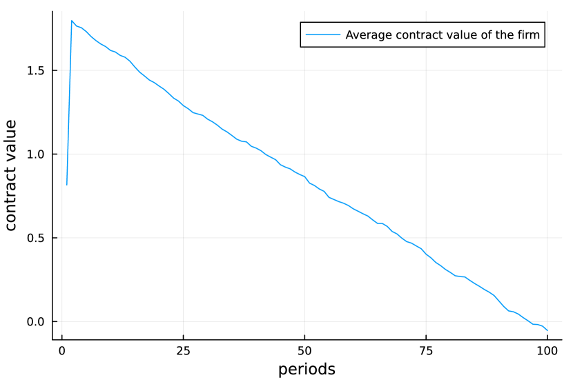
Figure 2: Average contract value

Figure 2 shows a series of sample means of $\overline{v}_{1}(\lambda_{n})$ for $n=1,2,\dots,100$. The $1000$ individuals are assumed to have the utility function

$$u(c)=\frac{1}{1+\gamma}(c+1)^{1+\gamma},$$

where $\gamma=-3$. The initial allocation weight $\lambda_{0}$ is set to $\lambda_{0}=50$ and the discount rate $\beta$ is set to $\beta=0.9$. The parameter $\gamma$ is set to $\gamma=-3$. In this case the planner chooses an allocation weight from $\lambda_{\text{min}}=19.128$ to $\lambda_{\text{max}}=166.375$. The income set $E$ is $E=\{0,1,2,3,4,5,6,7,8,9\}$. The random numbers are generated using the discrete probability distribution $P(e_{t}=0)=Pr(e_{t}=9)=0.025$, $P(e_{t}=1)=P(e_{t}=8)=0.045781$, $P(e_{t}=2)=P(e_{t}=7)=0.092762$, $P(e_{t}=3)=P(e_{t}=6)=0.148524$, $P(e_{t}=4)=Pr(e_{t}=5)=0.187933$.

The series of sample means in Figure 2 has a roughly increasing trend in the long run. The corresponding series of sample means of $\{\overline{v}_{2}(\lambda_{n})\}$ is shown in Figure 2. It clearly has a decreasing trend after about period $10$, although it remains positive until about period $90$. This property implies that the $\Gamma^{i}$ mechanism is not feasible.

To solve the last problem, the planner also considers intergenerational cooporation. Cooporation is achieved by simply entering the mechanism when it is their turn. For example, at the beginning of each period a new set of individuals of the same size enters the mechanism. In this way, the average contract value of the firm could remain positive in the long run.

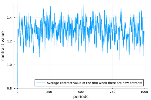
Figure 3: Average lifetime utilities

Figure 3 shows a series of sample means of $\overline{v}_{2}(\lambda_{n})$ for $n=1,\dots,100$, in the case where a thousand individuals join the mechanism in each period. The parameters are the same as in the figure 2. Since a decreasing trend in the firm’s contract values is offset by the revenues from the new entrants, the firm’s average contract value remains positive.

As one might expect, lifetime utilities are much better in $\Gamma^{i}$ than in the state of autarky. This result contrasts with the numerical results of Marcet and Marimon [1992], where the lifetime utility of agent 1 (manager) is higher in the state of autarky than in the state of the incentive contract with agent 2 (investor). This is probably because, first, Marcet and Marimon [1992] is a growth model with the assumption that capital, and hence the manager’s consumption, increases when the manager chooses the optimal level of investment. Second, since the transfers in the numerical example for incentive contracts in Marcet and Marimon [1992] are not competitive, the external financing contracts end up reducing agent 1’s allocation.

4 Discussion

Previous work using the promised utility approach [Green, 1987, Thomas and Worrall, 1990, Atkeson and Lucas, 1992, Phelan, 1998] shows that efficient allocations are possible at the cost of inequality in the absence of full information, or assuming a discounting factor of approximately $1$. In addition, other related studies based on the promised utility approach [Phelan, 2006] show that efficient resource allocation may require social rankings.

The approach in these studies is to manipulate the transfer function $\tau$ to be as efficient as possible at the expense of equality. Only individuals with the highest incomes remain in the highest contract value position in the next period, and contract values in the next period are discounted according to reported incomes. In the absence of such inequality in the future, individuals with higher incomes may prefer to misreport, which results in them receiving the higher transfers provided for individuals with lower incomes. Thus, the value of tomorrow’s contracts for lower income individuals must be reduced relative to their value today. As a result, the average contract value of individuals becomes a decreasing series.

However, the current study shows that incentivising truth-telling to achieve efficient allocation does not necessarily lead to inequality. The proposed mechanism simply shifts risks to the future periods. A similar limitation is that, in order to achieve efficiency, the proposed mechanism leads to a decreasing series of the average contract value of the firm. However, this could be solved naturally by adding new generations to the mechanism in each period. If this intergenerational cooperation is expected, the proposed mechanism is sustainable.

5 Conclusion

This paper presents an alternative solution to avoid the prediction of the previous work: if the incomes of infinitely lived individuals are unobservable, efficient allocations are achieved only at the cost of invoking permanent inequality, leading to an immiseration of society. The proposed inter-period transfer mechanism achieves within-period full insurance by postponing risks. It does not trade off equal opportunities to become wealthy. It could be sustained by intergenerational cooporation. The result sheds light on efficient resource allocation for sustainable societies with equal opportunities.

References

• Atkeson and Lucas [1992] Andrew Atkeson and Robert E. Lucas. On efficient distribution with private information. Review of Economic Studies, 59(3):427–453, 1992.
• Carrasco et al. [2019] Vinicius Carrasco, William Fuchs, and Satoshi Fukuda. From equals to despots: The dynamics of repeated decision making in partnerships with private information. Journal of Economic Theory, 182:402–432, 2019.
• Green [1987] Edward J. Green. Lending and the smoothing of uninsurable income. In Edward C. Prescott and Neil Wallace, editors, Contractual Arrangement for Intertemporal Trade, volume 1 of Minnesota Studies in Macroeconomics. University of Minnesota Press, Minneapolis, 1987.
• Marcet and Marimon [1992] Albert Marcet and Ramon Marimon. Communication, commitment, and growth. Journal of Economic Theory, 58(2):219–249, 1992.
• Phelan [1998] Christopher Phelan. On the long run implications of repeated moral hazard. Journal of Economic Theory, 79(2):174–191, 1998.
• Phelan [2006] Christopher Phelan. Opportunity and social mobility. Review of Economic Studies, 73(2):4870504, 2006.
• Thomas and Worrall [1990] Jonathan Thomas and Tim Worrall. Income fluctuation and asymmetric information: An example of repeated principal-agent problem. Jornal of Economic Theory, 51(2):367–390, 1990.