Polarized Raman Response of Two-Dimensional Quasiperiodic Antiferromagnets: Configuration-Interaction versus Green’s Function Approaches

Abstract

We study Raman response of Heisenberg antiferromagnets on the $\mathbf{C}_{\mathrm{5v}}$ Penrose and $\mathbf{C}_{\mathrm{8v}}$ Ammann-Beenker lattices within and beyond the Loudon-Fleury second-order perturbation scheme intending to explore optical features peculiar to quasiperiodic magnets. Within the Loudon-Fleury mechanism, we find one and only Raman-active mode of $\mathrm{E}_{2}$ symmetry without any dependence on linear incident and scattered polarizations. Beyond the Loudon-Fleury mechanism, two more symmetry species $\mathrm{A}_{1}$ and $\mathrm{A}_{2}$ are activated via dynamic ring exchange and chiral spin fluctuations, respectively, which can be extracted by the use of circular as well as linear polarizations. We employ Green’s functions on one hand and configuration-interaction wavefunctions on the other hand to calculate the multimagnon contributions to inelastic light scatterings. Demonstrating the great advantage of the configuration-interaction scheme, we reveal that a major portion of the Shastry-Shraiman fourth-order Raman intensity is mediated by multimagnon fluctuations.

A variety of quasiperiodic magnetic crystals [3, 4, 5, 6] have renewed the theoretical exploration of novel magnetism of geometric origin. The Penrose and Ammann-Beenker lattices in two dimensions attract much interest in this context. Their Ising [7, 8] and Heisenberg [9, 10, 11, 12] models were calculated by the linear spin-wave (SW) theory and Monte Carlo (MC) methods, whereas their Hubbard models [13, 14] were investigated within a mean-field approximation. In the context of inelastic-neutron-scattering experiments, SW findings for the dynamic structure factor of the Ammann-Beenker Heisenberg antiferromagnet reveal intriguing excitation features possibly due to the quasiperiodicity [10]; the coexistence of linear soft modes near the magnetic Bragg peaks at low frequencies, self-similar structures at intermediate frequencies, and flat bands at high frequencies. We may take further interest in inelastic light scatterings in quasiperiodic magnets, which strongly reflect their lattice symmetry and potentially bring brandnew information by virtue of the light polarization degrees of freedom.

Recent technical progress of manipulating optical lattices [15, 16, 17] also deserves special mention. Two-dimensional (2D) quasiperiodic potentials with five- [18] or eight-fold [19, 20] rotational symmetry were theoretically designed in terms of standing-wave lasers and indeed observed via Bragg diffraction [18, 16]. By trapping ultracold bosonic or fermionic atoms in optically tunable potentials, we can change the on-site interaction and tunneling energy to obtain various effective spin models [21]. There may be an extended-to-localized phase transition [22, 17] of a Bose-Einstein condensate, for instance.

Thus motivated, we study Raman responses of 2D quasiperiodic spin-$\frac{1}{2}$ Heisenberg antiferromagnets on the ${\mathbf{C}}_{\mathrm{5v}}$ Penrose [23, 24] and ${\mathbf{C}}_{\mathrm{8v}}$ Ammann-Beenker [25, 26] lattices, described by the Hamiltonian $\mathcal{H}=J\sum_{\langle i,j\rangle}{\bm{S}}_{i}\cdot{\bm{S}}_{j}\ (J>0),$ where $\sum_{\langle i,j\rangle}$ runs over all pairs of connected vertices. With their bipartite structures in mind, we introduce Holstein-Primakoff bosons [27] and expand the bosonic Hamiltonian in powers of the inverse spin magnitude $1/S$, denoting the terms of order $S^{m}$ by $\mathcal{H}^{(m)}$. When we decompose the quartic boson operators $\mathcal{H}^{(0)}$ into quadratic terms $\mathcal{H}_{\mathrm{BL}}^{(0)}$ and residual normal-ordered quartic interactions $:\mathcal{H}^{(0)}:$ using Wick’s theorem [28, 29], the up-to-$O(S^{0})$ bosonic Hamiltonian reads

$$\mathcal{H}=\mathcal{H}^{(2)}+\mathcal{H}^{(1)}+\mathcal{H}^{(0)}_{\mathrm{BL}}+:\mathcal{H}^{(0)}:\equiv\mathcal{H}_{\mathrm{BL}}+:\mathcal{H}^{(0)}:.$$ (1)

First we diagonalize the bilinear Hamiltonian $\mathcal{H}_{\mathrm{BL}}$ via the generalized Bogoliubov transformation [10, 30, 31],

$$\mathcal{H}_{\mathrm{BL}}=\sum_{m=0}^{2}E^{(m)}+\sum_{\sigma=\pm}\sum_{l_{\sigma}=1}^{L_{\sigma}}\varepsilon_{l_{\sigma}}^{\sigma}\alpha_{l_{\sigma}}^{\sigma\dagger}\alpha_{l_{\sigma}}^{\sigma};\ \sum_{\sigma=\pm}L_{\sigma}\equiv L,$$ (2)

where $E^{(2)}$ is the classical ground-state energy and $E^{(m)}$ ($m=1,0$) are the $O(S^{m})$ quantum corrections to it, while $\alpha_{l_{\sigma}}^{\sigma\dagger}$ creates an antiferromagnetic ($\sigma=+$) or ferromagnetic ($\sigma=-$) SW [32, 33] of energy $\varepsilon_{l_{\sigma}}^{\sigma}$ for the vacuum state $|0\rangle_{\mathrm{BL}}$, enhancing or reducing the ground-state magnetization, respectively [34, 35]. Then we take account of the two-body interactions $:\mathcal{H}^{(0)}:$ in two ways, i.e., Green’s function (GF) perturbative and configuration-interaction (CI) variational approaches.

Shastry and Shraiman [36, 37] formulated magnetic Raman scatterings in an antiferromagnetic insulator by perturbatively treating the single-band Hubbard model in the limit of sufficiently strong correlation $U$ compared to hopping $t$ [38]. With the electron band being half filled, the second-order vertex ${}^{[2]}\mathcal{R}$ results in the well-known Loudon-Fleury operator [39], consisting of pair exchange interactions ${\bm{S}}_{i}\cdot{\bm{S}}_{j}$, whereas the fourth-order vertices ${}^{[4]}\mathcal{R}$ contain three-spin scalar-chirality terms $\propto\bm{S}_{i}\cdot(\bm{S}_{j}\times\bm{S}_{k})$ and four-spin ring-exchange terms $\propto(\bm{S}_{i}\cdot\bm{S}_{j})(\bm{S}_{k}\cdot\bm{S}_{l})$ [40, 41, 42]. With varying incident photon frequency $\omega_{\mathrm{in}}$, ${}^{[2]}\mathcal{R}$ predominates in the far-resonant regime, $t\ll|U-\hbar\omega_{\mathrm{in}}|$, while ${}^{[4]}\mathcal{R}$’s are also of major importance in the near-resonant regime, $t\simeq|U-\hbar\omega_{\mathrm{in}}|$. The Raman operators are classified according to the number of their constituent spin operators, ${}^{[2n]}\mathcal{R}=\sum_{\tau=2}^{2n}{}_{\;\;\;\;\tau}^{[2n]}\mathcal{R}$ $(n=1,2)$, and each component can be expanded in $1/S$ in terms of the bosonic language,

$${}_{\;\;\;\;\tau}^{[2n]}\mathcal{R}=\sum_{m=0}^{\infty}{}_{\;\;\;\;\tau}^{[2n]}\mathcal{R}^{(\tau-m)}=\sum_{m=0}^{\infty}\sum_{l=0}^{m}{}_{\;\;\;\;\tau}^{[2n]}\mathcal{R}_{2l\mathrm{M}}^{(\tau-m)},$$ (3)

where ${}_{\;\;\;\;\tau}^{[2n]}\mathcal{R}^{(\tau-m)}$, consisting of $2l\,(0\leq l\leq m)$-magnon ($2l\mathrm{M}$) vertices, is of order $S^{\tau-m}$. Via the Bogoliubov transformation, (3) truncated at $m=2$, i.e., the up-to-$O(S^{0})$ vertices become

$$\mathcal{R}\simeq\sum_{n=1}^{1\,\mathrm{or}\,2}\sum_{l=0}^{2}{}^{[2n]}\mathcal{R}_{2l\mathrm{M}}=\sum_{n=1}^{1\,\mathrm{or}\,2}\sum_{\tau=2}^{2n}\sum_{l=0}^{2}\sum_{m=l}^{2}{}_{\;\;\;\;\tau}^{[2n]}\mathcal{R}_{2l\mathrm{M}}^{(\tau-m)},$$ (4)

where ${}_{\;\;\;\;\tau}^{[2n]}\mathcal{R}_{2l\mathrm{M}}^{(\tau-m)}$ are normal-ordered with respect to the quasiparticle magnon operators. ${}^{[2n]}\mathcal{R}_{0\mathrm{M}}$ merely contribute to elastic (Rayleigh) scatterings and are thus omitted hereafter.

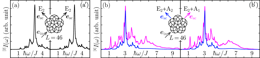
Figure 1: GF calculations of the Raman intensities ${}^{[p]}I(\omega)\equiv\sum_{l=1}^{2}{}^{[p]}I_{2l\mathrm{M}}(\omega)$ for the $L=46$ 2D Penrose lattice of ${\mathbf{C}}_{5\mathrm{v}}$ point symmetry in the Loudon-Fleury second-order ($p=2$) [(a) and (a^′)] and Shastry-Shraiman fourth-order ($p=4$) [(b) and (b^′)] perturbation schemes. ${}^{[p]}I_{2\mathrm{M}}(\omega)$ is obtained from (LABEL:E:1to4MGF(t)b) [51], while ${}^{[p]}I_{4\mathrm{M}}(\omega)$ is calculated in two ways, by the use of (LABEL:E:4MGF22) [51] [(a) and (b)] and (LABEL:E:4MGF31) [51] [(a^′) and (b^′)]. Two combinations of linear incident and scattered polarizations, $\phi_{-}=0,\pi/2$, are simulated. The Shastry-Shraiman perturbation parameter $t/(U-\hbar\omega_{\mathrm{in}})$ is set equal to $1/9$ and $9/10$ within [(a) and (a^′)] and beyond [(b) and (b^′)] the Loudon-Fleury scheme, respectively. Every spectral line is Lorentzian-broadened by a width of $0.1J$.

Putting $\mathcal{R}(t)\equiv e^{i\mathcal{H}t/\hbar}\mathcal{R}e^{-i\mathcal{H}t/\hbar}$ for any operator $\mathcal{R}$, we define the $2l\mathrm{M}$-mediated Raman intensities at absolute zero as [43]

$$\int_{-\infty}^{\infty}\frac{dt\,e^{i\omega t}}{2\pi\hbar L}\sum_{n,n^{\prime}=1}^{p/2}\langle 0|{}^{[2n]}\mathcal{R}_{2l\mathrm{M}}^{\dagger}(t)\,{}^{[2n^{\prime}]}\mathcal{R}_{2l\mathrm{M}}|0\rangle\equiv{}^{[p]}I_{2l\mathrm{M}}(\omega).$$ (5)

Once we find the exact ground state of the Heisenberg Hamiltonian, $\mathcal{H}|0\rangle=E_{0}|0\rangle$, the Loudon-Fleury ($p=2$) and Shastry-Shraiman ($p=4$) intensities can be exactly evaluated as [44, 45, 46, 47]

$${}^{[p]}I(\omega)=\int_{-\infty}^{\infty}\frac{dt\,e^{i\omega t}}{2\pi\hbar L}\sum_{n,n^{\prime}=1}^{p/2}\langle 0|{}^{[2n]}\mathcal{R}^{\dagger}(t)\,{}^{[2n^{\prime}]}\mathcal{R}|0\rangle=\frac{-1}{\pi L}\allowdisplaybreaks$$

$$\quad\times\sum_{n,n^{\prime}=1}^{p/2}\mathop{\mathrm{lim}}_{\eta\rightarrow+0}\mathrm{Im}\langle 0|{}^{[2n]}\mathcal{R}^{\dagger}\frac{1}{\hbar\omega+E_{0}+i\eta-\mathcal{H}}{}^{[2n^{\prime}]}\mathcal{R}|0\rangle$$ (6)

and may be approximated by the sum $\sum_{l=1}^{2}{}^{[p]}I_{2l\mathrm{M}}(\omega)$.

Magnon-magnon interactions significantly modify the Raman spectra [47, 48, 49, 50], because pair-exchange and multiple-spin cyclic-exchange Raman vertices, emergent within and beyond the Loudon-Fleury scheme, respectively, play qualitatively different roles in inelastic photon scatterings. First we demonstrate this by a renormalized perturbation theory [51]. In terms of the magnon GFs (LABEL:E:1to4MGF(t)b) and (LABEL:E:1to4MGF(t)d) [51], the $2l\mathrm{M}$-mediated Raman scattering intensities are calculated as [38]

$$\!\!\!{}^{[p]}I_{2l\mathrm{M}}(\omega)=-\mathrm{Im}\int_{-\infty}^{\infty}\frac{dt\,e^{i\omega t}}{i\pi\hbar L}\sum_{n,n^{\prime}=1}^{p/2}\langle 0|\mathcal{T}\,{}^{[2n]}\mathcal{R}_{2l\mathrm{M}}^{\dagger}(t)\,{}^{[2n^{\prime}]}\mathcal{R}_{2l\mathrm{M}}|0\rangle\allowdisplaybreaks$$

$$\!\!\!\qquad\quad\ \ \ \equiv-\mathrm{Im}\int_{-\infty}^{\infty}\frac{dt\,e^{i\omega t}}{\pi\hbar L}{}^{[p]}\mathcal{G}_{2l\mathrm{M}}(t);\allowdisplaybreaks$$

$$\!\!\!{}^{[p]}\mathcal{G}_{2\mathrm{M}}(t)=\sum_{k_{+},k_{-}^{\prime}}\sum_{l_{+},l_{-}^{\prime}}{}^{[p]}W_{k_{+}k_{-}^{\prime}}^{(2)\,*}G^{k_{+}k_{-}^{\prime}}_{l_{+}l_{-}^{\prime}}(t)\,{}^{[p]}W_{l_{+}l_{-}^{\prime}}^{(2)},\ {}^{[p]}\mathcal{G}_{4\mathrm{M}}(t)\allowdisplaybreaks$$

$$\!\!\!\ \ =\sum_{k_{+},k_{+}^{\prime},k_{-}^{\prime\prime},k_{-}^{\prime\prime\prime}}\sum_{l_{+},l_{+}^{\prime},l_{-}^{\prime\prime},l_{-}^{\prime\prime\prime}}{}^{[p]}X_{k_{+}k_{+}^{\prime}k_{-}^{\prime\prime}k_{-}^{\prime\prime\prime}}^{(7)\,*}G^{k_{+}k_{+}^{\prime}k_{-}^{\prime\prime}k_{-}^{\prime\prime\prime}}_{l_{+}l_{+}^{\prime}l_{-}^{\prime\prime}l_{-}^{\prime\prime\prime}}(t)\,{}^{[p]}X_{l_{+}l_{+}^{\prime}l_{-}^{\prime\prime}l_{-}^{\prime\prime\prime}}^{(7)},$$ (7)

where we numerically obtain the coefficients ${}^{[p]}W_{l_{+}l_{-}^{\prime}}^{(2)}$ and ${}^{[p]}X_{l_{+}l_{+}^{\prime}l_{-}^{\prime\prime}l_{-}^{\prime\prime\prime}}^{(7)}$. Since any perturbative renormalization is hardly tractable for more-than-3M GFs, we decompose 4M GFs into 2M GFs as (LABEL:E:4MGFsimeq2+2) [51] on one hand and into 3M and 1M GFs as (LABEL:E:4MGFsimeq3+1) [51] on the other hand. The renormalized 1M GFs reduce to the Hartree-Fock solutions (LABEL:E:Dyson) [51], whereas the 2M and 3M ones are calculated through ladder-approximation Bethe-Salpeter equations (LABEL:E:2lBS) [51] and (LABEL:E:3lBS) [51, 52], respectively.

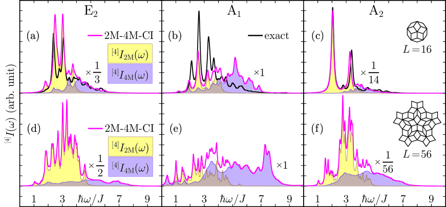
Figure 2: 2M-4M-CI calculations of the Shastry-Shraiman fourth-order Raman intensities ${}^{[4]}I(\omega)\equiv\sum_{l=1}^{2}{}^{[4]}I_{2l\mathrm{M}}(\omega)$ for the $L=16$ [(a) to (c)] and $L=56$ [(d) to (f)] 2D Penrose lattice of ${\mathbf{C}}_{5\mathrm{v}}$ point symmetry, the above three of which are compared with the exact solutions, where the perturbation parameter $t/(U-\hbar\omega_{\mathrm{in}})$ is set to $9/10$ and every spectral line is Lorentzian-broadened by a width of $0.1J$. The pure symmetry components are extracted from three polarization combinations, (15) with $\phi_{-}=0,\pi/2$ and (16) with $\sigma_{\mathrm{in}}\sigma_{\mathrm{sc}}=-1$. All the SW calculations of $I_{2l\mathrm{M}}(\omega)$ each are distinguishably colored.

The Raman operator is written as a rank-$2$ tensor dotted with the polarization vectors of the incident ($\bm{e}_{\mathrm{in}}$) and scattered ($\bm{e}_{\mathrm{sc}}$) photons [50, 53],

$${}^{[p]}\mathcal{R}=\sum_{\mu,\nu=x,y}e_{\mathrm{in}}^{\mu}{}^{[p]}\mathcal{R}^{\mu\nu}e_{\mathrm{sc}}^{\nu\,*},$$ (8)

where we set $\bm{e}_{\mathrm{in}}$ and $\bm{e}_{\mathrm{sc}}$ parallel to the lattice plane ($e_{\mathrm{in}}^{z}=e_{\mathrm{sc}}^{z}=0$) to reduce ${}^{[p]}\mathcal{R}$ to a $2\times 2$ matrix. In terms of the point symmetry group $\mathbf{P}$ of the lattice, this is rewritten as [54, 55]

$${}^{[p]}\mathcal{R}=\mathop{{\sum_{i}}^{\prime}}\sum_{\mu=1}^{d_{\varXi_{i}}^{\mathbf{P}}}E_{\varXi_{i}:\mu}^{\mathbf{P}}\,{}^{[p]}\mathcal{R}_{\varXi_{i}:\mu}^{\mathbf{P}},$$ (9)

where $\sum_{i}^{\prime}$ runs over the Raman-active irreducible representations $\varXi_{i}$ of $\mathbf{P}$, each with dimensionality $d_{\varXi_{i}}^{\mathbf{P}}$, and $E_{\varXi_{i}:\mu}^{\mathbf{P}}$ and $\mathcal{R}_{\varXi_{i}:\mu}^{\mathbf{P}}$ are the $\mu$th polarization-vector basis function and Raman vertex for $\varXi_{i}$, respectively. Since the ground state $|0\rangle$ is invariant under every symmetry operation of $\mathbf{P}$, any expectation value between Raman vertices of different symmetry species for it goes to zero [53, 54, 55, 56]. We can therefore classify the Raman intensities as to symmetry species,

$$\int_{-\infty}^{\infty}\frac{dt\,e^{i\omega t}}{2\pi\hbar L}\sum_{n,n^{\prime}=1}^{p/2}\langle 0|{}^{[2n]}\mathcal{R}_{\varXi_{i}:\mu}^{\mathbf{P}\,\dagger}(t)\,{}^{[2n^{\prime}]}\mathcal{R}_{\varXi_{i}:\mu}^{\mathbf{P}}|0\rangle\equiv{}^{[p]}I_{\varXi_{i}:\mu}^{\mathbf{P}}(\omega).$$ (10)

Considering that ${}^{[p]}I_{\varXi_{i}:1}^{\mathbf{P}}(\omega)={}^{[p]}I_{\varXi_{i}:\mu}^{\mathbf{P}}(\omega)$ $(\mu=2,\cdots,d_{\varXi_{i}}^{\mathbf{P}})$ for any multidimensional representation $\varXi_{i}$ [53, 54], we find

$${}^{[p]}I(\omega)=\mathop{{\sum_{i}}^{\prime}}{}^{[p]}I_{\varXi_{i}:1}^{\mathbf{P}}(\omega)\sum_{\mu=1}^{d_{\varXi_{i}}^{\mathbf{P}}}\bigl{|}E_{\varXi_{i}:\mu}^{\mathbf{P}}\bigr{|}^{2}.$$ (11)

When $\mathbf{P}=\mathbf{C}_{\mathrm{5v}}$, (9) contains two 1D and one 2D symmetry species [57], whose basis functions and vertices are given by

$$E_{\mathrm{A}_{1}:1}^{\mathbf{C}_{\mathrm{5v}}}=e_{\mathrm{in}}^{x}e_{\mathrm{sc}}^{x\,*}+e_{\mathrm{in}}^{y}e_{\mathrm{sc}}^{y\,*},\ E_{\mathrm{A}_{2}:1}^{\mathbf{C}_{\mathrm{5v}}}=e_{\mathrm{in}}^{x}e_{\mathrm{sc}}^{y\,*}-e_{\mathrm{in}}^{y}e_{\mathrm{sc}}^{x\,*},\allowdisplaybreaks$$

$$E_{\mathrm{E}_{2}:1}^{\mathbf{C}_{\mathrm{5v}}}=e_{\mathrm{in}}^{x}e_{\mathrm{sc}}^{y\,*}+e_{\mathrm{in}}^{y}e_{\mathrm{sc}}^{x\,*},\ E_{\mathrm{E}_{2}:2}^{\mathbf{C}_{\mathrm{5v}}}=e_{\mathrm{in}}^{x}e_{\mathrm{sc}}^{x\,*}-e_{\mathrm{in}}^{y}e_{\mathrm{sc}}^{y\,*},\allowdisplaybreaks$$ (12)

$${}^{[p]}\mathcal{R}_{\mathrm{A}_{1}:1}^{\mathbf{C}_{\mathrm{5v}}}=\frac{{}^{[p]}\mathcal{R}^{xx}+{}^{[p]}\mathcal{R}^{yy}}{2},\ {}^{[p]}\mathcal{R}_{\mathrm{A}_{2}:1}^{\mathbf{C}_{\mathrm{5v}}}=\frac{{}^{[p]}\mathcal{R}^{xy}-{}^{[p]}\mathcal{R}^{yx}}{2},\allowdisplaybreaks$$

$${}^{[p]}\mathcal{R}_{\mathrm{E}_{2}:1}^{\mathbf{C}_{\mathrm{5v}}}=\frac{{}^{[p]}\mathcal{R}^{xy}+{}^{[p]}\mathcal{R}^{yx}}{2},\ {}^{[p]}\mathcal{R}_{\mathrm{E}_{2}:2}^{\mathbf{C}_{\mathrm{5v}}}=\frac{{}^{[p]}\mathcal{R}^{xx}-{}^{[p]}\mathcal{R}^{yy}}{2}.$$ (13)

For the linear polarizations $\bm{e}_{\mathrm{in}/\mathrm{sc}}=(\cos\phi_{\mathrm{in}/\mathrm{sc}},\sin\phi_{\mathrm{in}/\mathrm{sc}},0)$, (12) reads $E_{\mathrm{A}_{1}:1}^{\mathbf{C}_{\mathrm{5v}}}=\cos\phi_{-}$, $E_{\mathrm{A}_{2}:1}^{\mathbf{C}_{\mathrm{5v}}}=\sin\phi_{-}$, $E_{\mathrm{E}_{2}:1}^{\mathbf{C}_{\mathrm{5v}}}=\sin\phi_{+}$, and $E_{\mathrm{E}_{2}:2}^{\mathbf{C}_{\mathrm{5v}}}=\cos\phi_{+}$ with $\phi_{\pm}\equiv\phi_{\mathrm{sc}}\pm\phi_{\mathrm{in}}$. Since ${}^{[2]}\mathcal{R}_{\mathrm{A}_{1}:1}^{\mathbf{C}_{\mathrm{5v}}}$ commutes with the Heisenberg Hamiltonian, the $\mathrm{A}_{1}$ species is Raman inactive within the Loudon-Fleury scheme. The $\mathrm{A}_{2}$ species is also Loudon-Fleury-Raman inactive. Since the Raman operator is time-reversal-invariant [37], the $(\bm{e}_{\mathrm{in}}\leftrightarrow\bm{e}_{\mathrm{sc}}^{*})$-exchange-antisymmetric basis function $E_{\mathrm{A}_{2}:1}^{\mathbf{C}_{\mathrm{5v}}}$ demands that ${}^{[p]}\mathcal{R}_{\mathrm{A}_{2}:1}^{\mathbf{C}_{\mathrm{5v}}}$ be also time-reversal-antisymmetric. The second-order pair-exchange Raman vertices are all time-reversal-invariant. ${}^{[2]}\mathcal{R}$ for the 2D Penrose lattice thus consists of one and only Raman-active species ${\mathrm{E}_{2}}$ to yield depolarized spectra,

$${}^{[2]}I(\omega)=\left(\bigl{|}E_{\mathrm{E}_{2}:1}^{\mathbf{C}_{\mathrm{5v}}}\bigr{|}^{2}+\bigl{|}E_{\mathrm{E}_{2}:2}^{\mathbf{C}_{\mathrm{5v}}}\bigr{|}^{2}\right)\,{}^{[2]}I_{\mathrm{E}_{2}:1}^{\mathbf{C}_{\mathrm{5v}}}(\omega)={}^{[2]}I_{\mathrm{E}_{2}:1}^{\mathbf{C}_{\mathrm{5v}}}(\omega),$$ (14)

as is shown in Figs. 1(a) and 1(a^′). This is no longer the case with higher-order Raman vertices. ${}^{[4]}\mathcal{R}_{\mathrm{A}_{1}:1}^{\mathbf{C}_{\mathrm{5v}}}$ contains ring-exchange spin fluctuations $(\bm{S}_{i}\cdot\bm{S}_{j})(\bm{S}_{k}\cdot\bm{S}_{l})$ incommutable with the Heisenberg Hamiltonian, whereas ${}^{[4]}\mathcal{R}_{\mathrm{A}_{2}:1}^{\mathbf{C}_{\mathrm{5v}}}$ comprises chiral spin fluctuations ${\bm{S}}_{i}\cdot({\bm{S}}_{j}\times{\bm{S}}_{k})$ breaking the time-reversal symmetry, both of which drive the fourth-order Raman response to depend on the light polarization,

$${}^{[4]}I(\omega)={}^{[4]}I_{\mathrm{E}_{2}:1}^{\mathbf{C}_{\mathrm{5v}}}(\omega)+{}^{[4]}I_{\mathrm{A}_{1}:1}^{\mathbf{C}_{\mathrm{5v}}}(\omega)\cos^{2}\phi_{-}+{}^{[4]}I_{\mathrm{A}_{2}:1}^{\mathbf{C}_{\mathrm{5v}}}(\omega)\sin^{2}\phi_{-},$$ (15)

as is demonstrated in Figs. 1(b) and 1(b^′).

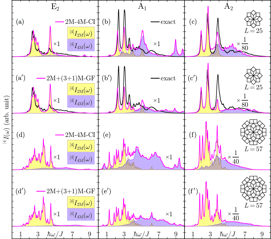
Figure 3: 2M-4M-CI [(a) to (f)] and $2\mathrm{M}+4\mathrm{M}$ [approximated by (LABEL:E:4MGF31)]-GF [(a^′) to (f^′)] calculations of ${}^{[4]}I(\omega)\equiv\sum_{l=1}^{2}{}^{[4]}I_{2l\mathrm{M}}(\omega)$ for the $L=25$ and $L=57$ 2D Ammann-Beenker lattice of ${\mathbf{C}}_{8\mathrm{v}}$ point symmetry, the above six of which are compared with the exact solutions. All other details are the same as Fig. 2.

Figures 1(a) and 1(a^′) present almost the same observations, while Figs. 1(b) and 1(b^′) show artificial differences at $\hbar\omega\gtrsim 5J$. Since we cannot directly evaluate more-than-3M GFs in practice, ${}^{[4]}I(\omega)$ and more generally Raman responses beyond the Loudon-Fleury scheme, containing significant multimagnon contributions, are much harder to reliably calculate in terms of GFs than ${}^{[2]}I(\omega)$ obtainable from the established Bethe-Salpeter equation. Even though we can calculate 3M GFs, for instance, there may be some different Bethe-Salpeter-like manners of renormalization [51, 58] to complicate matters further. In order to reliably evaluate the role of multimagnon scatterings in novel Raman responses beyond the Loudon-Fleury scheme, we propose an alternative approach utilizing CI variational wavefunctions [59]. Once we proceed to the fourth-order perturbation scheme, the polarized Raman spectra (15) for linearly polarized components of the incident and scattered field amplitudes are inadequate to identify all the three Raman-active symmetry species, and therefore, we consider circularly polarized components of them as well [60, 61]. For the incident and scattered fields of circular polarizations, $\bm{e}_{\mathrm{in}/\mathrm{sc}}=(1,\sigma_{\mathrm{in}/\mathrm{sc}}i,0)/\sqrt{2}$, (12) reads $E_{\mathrm{A}_{1}:1}^{\mathbf{C}_{\mathrm{5v}}}=(1+\sigma_{\mathrm{in}}\sigma_{\mathrm{sc}})/2$, $E_{\mathrm{A}_{2}:1}^{\mathbf{C}_{\mathrm{5v}}}=-i(\sigma_{\mathrm{in}}+\sigma_{\mathrm{sc}})/2$, $E_{\mathrm{E}_{2}:1}^{\mathbf{C}_{\mathrm{5v}}}=i(\sigma_{\mathrm{in}}-\sigma_{\mathrm{sc}})/2$, and $E_{\mathrm{E}_{2}:2}^{\mathbf{C}_{\mathrm{5v}}}=(1-\sigma_{\mathrm{in}}\sigma_{\mathrm{sc}})/2$ to yield the second- and fourth-order Raman responses

$${}^{[2]}I(\omega)=(1-\sigma_{\mathrm{in}}\sigma_{\mathrm{sc}})\,{}^{[2]}I_{\mathrm{E}_{2}:1}^{\mathbf{C}_{\mathrm{5v}}}(\omega),\ {}^{[4]}I(\omega)=(1-\sigma_{\mathrm{in}}\sigma_{\mathrm{sc}})\allowdisplaybreaks$$

$$\quad\times{}^{[4]}I_{\mathrm{E}_{2}:1}^{\mathbf{C}_{\mathrm{5v}}}(\omega)+\frac{1+\sigma_{\mathrm{in}}\sigma_{\mathrm{sc}}}{2}\left[{}^{[4]}I_{\mathrm{A}_{1}:1}^{\mathbf{C}_{\mathrm{5v}}}(\omega)+{}^{[4]}I_{\mathrm{A}_{2}:1}^{\mathbf{C}_{\mathrm{5v}}}(\omega)\right].$$ (16)

Substituting (16) with $\sigma_{\mathrm{in}}\sigma_{\mathrm{sc}}=-1$ into (15) with $\phi_{-}=0$ or $\phi_{-}=\pi/2$ reveals all the symmetry species separately.

A CI wavefunction generally consists of a linear combination of Hartree-Fock Slater determinants [62, 63], including a certain set of quasiparticle excited states as well as the ground state $|0\rangle_{\mathrm{BL}}$. In our 2M-4M-CI scheme, the Hilbert space in which the bosonic Hamiltonian (1) operates is spanned by the up-to-4M $N_{\mathrm{CI}}$ basis states (LABEL:E:CIBasisSets0M)–(LABEL:E:CIBasisSets4M) [59]. In terms of the variationally corrected eigenstates and eigenvalues of the 2M-4M-CI Hamiltonian (LABEL:E:CIHV(1)V(4)V(9)) [59], the $2l\mathrm{M}$-mediated Raman scattering intensities read

$$\!\!\!{}^{[p]}I_{2l\mathrm{M}}(\omega)=\frac{1}{L}\!\sum_{\nu=0}^{N_{\mathrm{CI}}-1}\!\left|\langle\nu|\sum_{n=1}^{p/2}{}^{[2n]}\mathcal{R}_{2l\mathrm{M}}|0\rangle\right|^{2}\!\delta(\hbar\omega-\varepsilon_{\nu}+\varepsilon_{0}).$$ (17)

We verify the CI evaluation (17) in Fig. 2. The CI findings for the $\mathrm{E}_{2}$ and $\mathrm{A}_{2}$ symmetry species are in very good agreement with the exact solutions obtained by a recursion method based on the Lanczos algorithm [64, 65]. While the $\mathrm{E}_{2}$ scattering is Loudon-Fleury-Raman active and arises chiefly from pair-exchange spin fluctuations, a nonnegligible portion of this scattering intensity is mediated by 4M fluctuations, as is revealed by our CI scheme. While the $\mathrm{A}_{2}$ scattering intensity is small compared to the other symmetries, it is so interesting as to allow for directly observing the chiral spin fluctuations $\bm{S}_{i}\cdot(\bm{S}_{j}\times\bm{S}_{k})$ [60]. The spin-chirality-driven $\mathrm{A}_{2}$ Raman response is emergent in the honeycomb and kagome lattices consisting of nonparallelograms but impossible in the square and triangular lattices comprising rhombuses [40]. The present scattering of $\mathrm{A}_{2}$ symmetry owes to the quasiperiodic geometry [66] whose rank $D$, i.e., the smallest number of wavevectors that can span the whole diffraction pattern of the crystal by their integral linear combinations, is larger than the actual physical dimension $d$. The $d=2$ Penrose and Ammann-Beenker lattices have the same indexing dimension $D=4$. Our CI scheme well reproduces the $\mathrm{A}_{1}$ exact solution as well but somewhat overestimates its 4M spectral weight. This is because the $\mathrm{A}_{1}$ symmetry species becomes Raman active due to ring exchange interactions such as $S_{i}^{+}S_{j}^{-}S_{k}^{+}S_{l}^{-}$, $S_{i}^{+}S_{j}^{-}S_{k}^{z}S_{l}^{z}$, and $S_{i}^{z}S_{j}^{z}S_{k}^{z}S_{l}^{z}$, the latter two of which are essentially described by six or more Holstein-Primakoff bosons and therefore sensitive to the Hamiltonian of $O(S^{-1})$.

What will happen to clusters without ${\mathbf{C}}_{5\mathrm{v}}$ symmetry? The $\mathrm{A}_{1}$ and $\mathrm{A}_{2}$ symmetry species remain Loudon-Fleury-Raman inactive, considering that ${}^{[2]}\mathcal{R}_{\mathrm{A}_{1}:1}^{\mathbf{C}_{\mathrm{5v}}}$ is commutable with the Heisenberg Hamiltonian and ${}^{[2]}\mathcal{R}_{\mathrm{A}_{2}:1}^{\mathbf{C}_{\mathrm{5v}}}$ is time-reversal-invariant regardless of the size and shape of clusters, whereas the Loudon-Fleury-Raman response ${}^{[2]}I(\omega)=\sum_{\mu=1}^{2}\bigl{|}E_{\mathrm{E}_{2}:\mu}^{\mathbf{P}}\bigr{|}^{2}{}^{[2]}I_{\mathrm{E}_{2}:\mu}^{\mathbf{P}}(\omega)$ is no longer perfectly depolarized without the equality ${}^{[p]}I_{\mathrm{E}_{2}:1}^{\mathbf{P}}(\omega)={}^{[p]}I_{\mathrm{E}_{2}:2}^{\mathbf{P}}(\omega)$. However, the polarization dependence disappears in the thermodynamic limit and it is already faint in such medium-sized clusters of $L\gtrsim 50$. Size dependence of the Raman spectra is further demonstrated in Supplemental Material [67].

Figure 3 shows comparative CI and GF calculations of the 2D Ammann-Beenker lattice. Even though we set $\mathbf{P}$ to $\mathbf{C}_{\mathrm{8v}}$ in (11), the second- and fourth-order Raman responses remain the same as (14), (15) and (16). Depolarization of ${}^{[2]}I(\omega)$ occurs in a certain class of periodic planar magnets as well, including Heisenberg antiferromagnets on the triangular [50] and kagome [40, 68] lattices and Kitaev spin liquids on the pure [69] and decorated [55] honeycomb lattices. In these lattice geometries, the two polarization-vector basis functions $e_{\mathrm{in}}^{x}e_{\mathrm{sc}}^{y\,*}+e_{\mathrm{in}}^{y}e_{\mathrm{sc}}^{x\,*}$ and $e_{\mathrm{in}}^{x}e_{\mathrm{sc}}^{x\,*}-e_{\mathrm{in}}^{y}e_{\mathrm{sc}}^{y\,*}$ span such a 2D irreducible representation as to be one and only Raman-active symmetry species. This criterion is met by 2D lattices with certain rotational symmetry [57], including periodic ones of triangular geometry and all noncrystallographic—in the conventional sense—ones [70, 71].

Figure 3 reveals our CI scheme to be much superior to the conventional GF approach. Indirect evaluation of the 4M GFs cannot reproduce the significant 4M-mediated scattering intensity in general. The spin-chirality-driven $\mathrm{A}_{2}$ scattering intensity is especially misunderstood by the GF approach. Indeed low-energy peaks are almost of 2M character, but high-energy ones clearly owe to both 2M and 4M scatterings, as is revealed by the CI calculations. The inaccurate 4M GFs are totally ignorant of the mixed character of these $\mathrm{A}_{2}$ scattering peaks and such is the case with every symmetry species. The essential features of all the calculational schemes developed are further demonstrated in Supplemental Material [67].

We have demonstrated the advantages of CI over GF in analyzing Raman scattering intensities according to mediating magnons. Once we go beyond the Loudon-Fleury second-order perturbation scheme, or sometimes even within it, we will find out any spectral weight of multimagnon character correctly only by evaluating the Raman correlation functions ${}^{[p]}\mathcal{G}_{2l\mathrm{M}}(t)$ directly. Real-frequency dynamic quantities cannot be obtained directly from path-integral calculations such as quantum MC (QMC) findings. Relevant imaginary-time correlation functions have to be first calculated and then continued to real frequency. Laplace transforms are difficult to invert numerically and maximum-entropy analytic continuation, for instance, of QMC data is not necessarily successful even for small periodic clusters [47]. Under such circumstances, our elaborate CI approach can open up a new path of calculating dynamic properties. In terms of its ability to clarify what kind of intermediate states are essential in which scattering channel, we note that a newly developed representation theory of the quantum affine Lie algebra for the spin-$\frac{1}{2}$ XXZ infinite chain [72, 73] opened the door to a full understanding of its dynamics. We are aware of how much percentage of its total structure factor intensity two- and four-spinon intermediate states contribute [74, 75]. Dynamic spin structure factors of quasiperiodic magnets [10] are also analyzable in full detail with the present CI scheme.

We are grateful to J. Ohara for his critical comments on our coding. This work is supported by JSPS KAKENHI Grant Number 22K03502.

References

• [1]
• [2] yamamoto@phys.sci.hokudai.ac.jp
• [3] B. Charrier and D. Schmitt, J. Magn. Magn. Mater. 171, 106 (1997).
• [4] I. R. Fisher, K. O. Cheon, A. F. Panchula, P. C. Canfield, M. Chernikov, H. R. Ott, and K. Dennis, Phys. Rev. B 59, 308 (1999).
• [5] T. J. Sato, H. Takakura, A. P. Tsai, K. Shibata, K. Ohoyama, and K. H. Andersen, Phys. Rev. B 61, 476 (2000).
• [6] T. J. Sato, H. Takakura, A. P. Tsai, and K. Shibata, Phys. Rev. B 73, 054417 (2006).
• [7] Y. Okabe and K. Niizeki, J. Phys. Soc. Jpn. 57, 16 (1988).
• [8] Y. Komura and Y. Okabe, J. Phys. Soc. Jpn. 85, 044004 (2016).
• [9] S. Wessel, A. Jagannathan, and S. Haas, Phys. Rev. Lett. 90, 177205 (2003).
• [10] S. Wessel and I. Milat, Phys. Rev. B 71, 104427 (2005).
• [11] A. Jagannathan, A. Szallas, S. Wessel, and M. Duneau, Phys. Rev. B 75, 212407 (2007).
• [12] A. Szallas and A. Jagannathan, Phys. Rev. B 77, 104427 (2008).
• [13] A. Koga and H. Tsunetsugu, Phys. Rev. B 96, 214402 (2017).
• [14] A. Koga, Phys. Rev. B 102, 115125 (2020).
• [15] L. Guidoni, C. Triché, P. Verkerk, and G. Grynberg, Phys. Rev. Lett. 79, 3363 (1997).
• [16] K. Viebahn, M. Sbroscia, E. Carter, J.-C. Yu, and U. Schneider, Phys. Rev. Lett. 122, 110404 (2019).
• [17] M. Sbroscia, K. Viebahn, E. Carter, J.-C. Yu, A. Gaunt, and U. Schneider, Phys. Rev. Lett. 125, 200604 (2020).
• [18] L. Sanchez-Palencia and L. Santos, Phys. Rev. A 72, 053607 (2005).
• [19] A. Jagannathan and M. Duneau, Europhys. Lett. 104, 66003 (2013).
• [20] A. Jagannathan and M. Duneau, Eur. Phys. J. B 87, 149 (2014).
• [21] L.-M. Duan, E. Demler, and M. D. Lukin, Phys. Rev. Lett. 91, 090402 (2003).
• [22] D. Johnstone, P. Öhberg, and C. W. Duncan, Phys. Rev. A 100, 053609 (2019).
• [23] N. G. de Bruijn, Indag. Math. Proc. Ser. A 84, 39 (1981).
• [24] N. G. de Bruijn, Indag. Math. Proc. Ser. A 84, 53 (1981).
• [25] J. E. S. Socolar, Phys. Rev. B 39, 10519 (1989).
• [26] M. Baake and D. Joseph, Phys. Rev. B 42, 8091 (1990).
• [27] T. Holstein and H. Primakoff, Phys. Rev. 58, 1098 (1940).
• [28] Y. Noriki and S. Yamamoto, J. Phys. Soc. Jpn. 86, 034714 (2017).
• [29] S. Yamamoto and Y. Noriki, Phys. Rev. B 99, 094412 (2019).
• [30] R. M. White, M. Sparks, and I. Ortenburger, Phys. Rev. 139, A450 (1965).
• [31] See Section S1 in Supplemental Material, where the up-to-$O(S^{0})$ bosonic Hamiltonian $\sum_{m=0}^{2}\mathcal{H}^{(m)}$ is decomposed into $\mathcal{H}_{\mathrm{BL}}$ and $:\mathcal{H}^{(0)}:$, the diagonalization of $\mathcal{H}_{\mathrm{BL}}$ is demonstrated, and $:\mathcal{H}^{(0)}:$ is expressed in terms of the quasiparticle magnon operators.
• [32] S. Yamamoto, T. Fukui, K. Maisinger, and U. Schollwöck, J. Phys.: Condens. Matter 10, 11033 (1998).
• [33] S. Yamamoto, Phys. Rev. B 69, 064426 (2004).
• [34] S. Brehmer, H.-J. Mikeska, and S. Yamamoto, J. Phys.: Condens. Matter 9, 3921 (1997).
• [35] S. Yamamoto and T. Fukui, Phys. Rev. B 57, 14008(R) (1998).
• [36] B. S. Shastry and B. I. Shraiman, Phys. Rev. Lett. 65, 1068 (1990).
• [37] B. S. Shastry and B. I. Shraiman, Int. J. Mod. Phys. B 5, 365 (1991).
• [38] See Section S2 in Supplemental Material, where magnetic Raman scatterings are derived from the half-filled single-band Hubbard model.
• [39] P. A. Fleury and R. Loudon, Phys. Rev. 166, 514 (1968).
• [40] W.-H. Ko, Z.-X. Liu, T.-K. Ng, and P. A. Lee, Phys. Rev. B 81, 024414 (2010).
• [41] F. Michaud, F. Vernay, and F. Mila, Phys. Rev. B 84, 184424 (2011).
• [42] T. Inoue and S. Yamamoto, Phys. Status Solidi B 257, 2000118 (2020).
• [43] While any finite cluster lie in the magnon vacuum at absolute zero, it is not necessarily the case with infinite lattices. In the thermodynamic limit of Heisenberg antiferromagnets on the Penrose and Ammann-Beenker lattices, Goldstone magnons may appear even at absolute zero. In such a case, every conventional spin-wave theory should be modified. [28, 29] Note that $\langle 0|{}^{[2n]}\mathcal{R}_{2l\mathrm{M}}^{\dagger}(t)\,{}^{[2n^{\prime}]}\mathcal{R}_{2l^{\prime}\mathrm{M}}|0\rangle=0$ unless $l=l^{\prime}$ not only for $|0\rangle=|0\rangle_{\mathrm{BL}}$ but also for any ground state $|0\rangle$ corrected by the quartic interaction $:\mathcal{H}^{(0)}:$ perturbatively or variationally.
• [44] F. Lema, J. Eroles, C. D. Batista, and E. R. Gagliano, Phys. Rev. B 55, 15295 (1997).
• [45] J. Eroles, C. D. Batista, S. B. Bacci, and E. R. Gagliano, Phys. Rev. B 59, 1468 (1999).
• [46] F. Nori, R. Merlin, S. Haas, A. W. Sandvik, and E. Dagotto, Phys. Rev. Lett. 75, 553 (1995).
• [47] A. W. Sandvik, S. Capponi, D. Poilblanc, and E. Dagotto, Phys. Rev. B 57, 8478 (1998).
• [48] C. M. Canali and S. M. Girvin, Phys. Rev. B 45, 7127 (1992).
• [49] A. V. Chubukov and D. M. Frenkel, Phys. Rev. B 52, 9760 (1995).
• [50] N. Perkins and W. Brenig, Phys. Rev. B 77, 174412 (2008).
• [51] See Section S3 in Supplemental Material, where we explain our ladder approximation for multimagnon GFs and give them in the Lehmann representation.
• [52] A. Carbone, A. Cipollone, C. Barbieri, A. Rios, and A. Polls, Phys. Rev. C 88, 054326 (2013).
• [53] B. Perreault, J. Knolle, N. B. Perkins, and F. J. Burnell, Phys. Rev. B 92, 094439 (2015).
• [54] T. Kimura and S. Yamamoto, Phys. Rev. B 101, 214411 (2020).
• [55] S. Yamamoto and T. Kimura, J. Phys. Soc. Jpn. 89, 063701 (2020).
• [56] T. P. Devereaux and R. Hackl, Rev. Mod. Phys. 79, 175 (2007).
• [57] See Section S4 in Supplemental Material, where the Raman operator in two dimensions is decomposed into symmetry-definite components and the dimensionality of each symmetry species is discussed.
• [58] C. Barbieri, D. Van Neck, and W. H. Dickhoff, Phys. Rev. A 76, 052503 (2007).
• [59] See Section S5 in Supplemental Material, where we explain our CI scheme and give the CI Hamiltonian.
• [60] P. E. Sulewski, P. A. Fleury, K. B. Lyons, and S-W. Cheong, Phys. Rev. Lett. 67, 3864 (1991).
• [61] R. H. Lehmberg, M. F. Wolford, J. L. Weaver, D. Kehne, S. P. Obenschain, D. Eimerl, and J. P. Palastro, Phys. Rev. A 102, 063530 (2020).
• [62] J. Ohara and S. Yamamoto, Phys. Rev. B 73, 045122 (2006).
• [63] S. Yamamoto, Phys. Rev. B 78, 235205 (2008).
• [64] V. S. Viswanath and G. Müller, The Recursion Method (Springer, Berlin, 1994).
• [65] S. Yamamoto, Physica B 481, 224 (2016).
• [66] R. Lifshitz, Z. Kristallogr. 222, 313 (2007).
• [67] See Section S6 in Supplemental Material, where we show CI and GF calculations of ${}^{[4]}I(\omega)\equiv\sum_{l=1}^{2}{}^{[4]}I_{2l\mathrm{M}}(\omega)$ for various 2D Penrose and Ammann-Beenker clusters.
• [68] O. Cépas, J. O. Haerter, and C. Lhuillier, Phys. Rev. B 77, 172406 (2008).
• [69] J. Knolle, G.-W. Chern, D. L. Kovrizhin, R. Moessner, and N. B. Perkins, Phys. Rev. Lett. 113, 187201 (2014).
• [70] D. Shechtman, I. Blech, D. Gratias, and J. W. Cahn, Phys. Rev. Lett. 53, 1951 (1984).
• [71] S. Van Smaalen, Cryst. Rev. 4, 79 (1995).
• [72] B. Davies, O. Foda, M. Jimbo, T. Miwa, and A. Nakayashiki, Commun. Math. Phys. 151, 89 (1993).
• [73] A. Abada, A. H. Bougourzi, and B. Si-Lakhal, Nucl. Phys. B 497, 733 (1997).
• [74] J.-S. Caux and R. Hagemans, J. Stat. Mech. (2006) P12013.
• [75] M. Mourigal, M. Enderle , A. Klöpperpieper, J.-S. Caux, A. Stunault, and H. M. Rønnow, Nature Phys. 9, 435 (2013). blank blank