Magnetism, rotation, and nonthermal emission in cool stars

Stellar dynamos generate magnetic fields that are of fundamental importance to the variability and evolution of Sun-like and low-mass stars, and for the development of their planetary systems. As a key to understanding stellar dynamos, empirical relations between stellar parameters and magnetic fields are required for comparison to ab initio predictions from dynamo models. We report measurements of surface-average magnetic fields in 292 M dwarfs from a comparison with radiative transfer calculations; for 260 of them, this is the first measurement of this kind. Our data were obtained from more than 15,000 high-resolution spectra taken during the CARMENES project. They reveal a relation between average field strength, $\langle B\rangle$, and Rossby number, $Ro$, resembling the well-studied rotation-activity relation. Among the slowly rotating stars, we find that magnetic flux, $\Phi_{\textrm{B}}$, is proportional to rotation period, $P$, and among the rapidly rotating stars that average surface fields do not grow significantly beyond the level set by the available kinetic energy. Furthermore, we find close relations between nonthermal coronal X-ray emission, chromospheric H$\alpha$ and Ca H&K emission, and magnetic flux. Taken together, these relations demonstrate empirically that the rotation-activity relation can be traced back to a dependence of the magnetic dynamo on rotation. We advocate the picture that the magnetic dynamo generates magnetic flux on the stellar surface proportional to rotation rate with a saturation limit set by the available kinetic energy, and we provide relations for average field strengths and nonthermal emission that are independent of the choice of the convective turnover time. We also find that Ca H&K emission saturates at average field strengths of $\langle B\rangle\approx 800$ G while H$\alpha$ and X-ray emission grow further with stronger fields in the more rapidly rotating stars. This is in conflict with the coronal stripping scenario predicting that in the most rapidly rotating stars coronal plasma would be cooled to chromospheric temperatures.

1 Introduction

Sun-like and low-mass stars generate magnetic fields through a hydromagnetic dynamo operating in their interiors (Parker, 1955; Charbonneau, 2013). The stellar dynamo is believed to transform the kinetic energy, $E_{\textrm{kin}}$, of the star’s turbulent convective motion into magnetic energy, $E_{\textrm{B}}$. In analogy to the Sun, starspots and stellar activity are believed to be a consequence of the emergence of magnetic flux at the stellar surface (e.g., Cameron & Schüssler, 2015; Brun & Browning, 2017). Heating in the stellar corona and chromosphere is closely related to magnetic flux (Pevtsov et al., 2003; Güdel, 2004), and magnetically active regions cause most of the stellar energy output variation on timescales ranging from minutes to centuries (Fröhlich & Lean, 2004).

Magnetic fields determine the variability and rotational evolution of main-sequence stars as well as the evolution of planetary systems. The relation between angular momentum loss and age yields a predictable evolution of stellar rotation and can provide estimates for stellar age from rotation measurements (Skumanich, 1972), a method called gyrochronology (Barnes, 2003). This spin-down mechanism acts most effectively in young stars and, over time, transforms them into old field stars with terminal rotation rates that are mass-dependent (McQuillan et al., 2014). Magnetic activity influences planetary evolution through the amount of high-energy radiation emitted during the phase when the planetary atmosphere is young because intense high-energy radiation and winds can evaporate the atmosphere of a planet in a close orbit (Sanz-Forcada et al., 2011; Johnstone et al., 2015). Magnetic fields and their variability are among the main obstacles for the radial velocity detection of low-mass planets (Reiners et al., 2013; Lisogorskyi et al., 2020; Haywood et al., 2020; Crass et al., 2021).

It is often suggested that the well-established stellar activity-rotation relation (e.g., Skumanich, 1972; Noyes et al., 1984; Pizzolato et al., 2003; Wright et al., 2011, 2018; Reiners et al., 2014) is a causal consequence of a hydromagnetic dynamo generating stronger magnetic fields in more rapidly rotating stars. The influence of rotation on convective motion is often expressed in terms of the Rossby number, $Ro=P/\tau$, the ratio between rotation period, $P$, and convective turnover time, $\tau$; chromospheric and coronal emission are observed to saturate in stars rotating more rapidly than $Ro\approx 0.1$. Slowly rotating stars ($Ro\ga 0.1$) emit chromospheric and coronal emission in approximate proportion to the inverse of the rotational period squared, $P^{-2}$, which leads to a weakening of stellar activity with age because of angular momentum loss. A mild dependence between X-ray emission and rotation is also observed in the saturated regime (Pizzolato et al., 2003; Reiners et al., 2014; Magaudda et al., 2020).

There is some direct evidence of the magnetic dynamo showing a similar dependence on rotation; the magnetic energy generated in rapidly rotating planets and stars is approximately limited by kinetic energy flux from convection (Christensen et al., 2009), and evidence for saturation in magnetic field strength exists from semi-empirical methods (Reiners et al., 2009a) and from detailed modeling in a limited sample (Shulyak et al., 2017). Furthermore, observations in very active M dwarfs reveal a relation between the field strength and rotation rate (Shulyak et al., 2017, 2019; Kochukhov, 2021), and observations of large-scale surface magnetic fields from Zeeman Doppler imaging (ZDI) show a similar relation (Vidotto et al., 2014).

A major challenge in predicting stellar magnetic field strengths is the broad range of timescales and length-scales involved, rendering detailed simulations of stellar convection impractical (Kupka & Muthsam, 2017). Instead, simplified models approximate the effects of turbulent convection, rotation, and Lorentz force feedback (Brun & Browning, 2017). For example, a balance between Coriolis, buoyancy, and Lorentz forces (MAC balance) leads to $E_{\textrm{B}}\sim E_{\textrm{kin}}/Ro$. On the other hand, a balance between advection and Lorentz forces results in magnetic fields in equipartition with convective kinetic energy. Scaling relations between magnetic dynamo efficiency and luminosity or rotation rate can in principle be estimated from models (e.g., Augustson et al., 2019), but the extent to which such simplified models can be compared to physical objects remains unclear. Furthermore, direct magnetic field measurements and the range of stellar parameters covered by observations have so far not provided enough empirical evidence to guide dynamo models, especially in slowly rotating stars.

The signatures of magnetism on surfaces of Sun-like and low-mass stars are very subtle. The most direct diagnostic of stellar magnetic fields is the Zeeman effect (e.g., Landi Degl’Innocenti & Landolfi, 2004; Donati & Landstreet, 2009; Reiners, 2012; Kochukhov, 2021). In general, it can be observed in polarized or in unpolarized light. Measurements in polarized light can detect the distribution of very weak fields on the order of a few Gauss. The analysis of circularly polarized light alone is prone to cancellation effects, but the measurement of linearly polarized light is very demanding. Often, deconvolution techniques are employed to construct average line profiles with very high signal-to-noise ratios (S/N) (e.g., Semel, 1989; Semel et al., 1993; Rosén et al., 2015). Unpolarized light can potentially reveal the full and unbiased magnetic field including very small-scale components, but here averaging spectral lines to boost the signal is not possible, and line formation must be modeled in great detail (see Kochukhov, 2021). Direct measurement of the surface-average magnetic field, $\langle B\rangle$, therefore requires exceptionally high S/N (at high spectral resolution) plus sophisticated radiative transfer calculations that can model polarization. In consequence, only a limited number of average field measurements based on detailed profile modeling exist, and no empirical relation is known between magnetic fields, fundamental stellar parameters, and rotation. On the theory side, ab initio predictions about stellar magnetic fields are very challenging (Brun & Browning, 2017), and empirical information about magnetic fields could help identify the parameter space in which stellar dynamos can operate.

Collecting data that meet the high requirements for average magnetic field measurements in a sizeable sample of low-mass stars is a challenge that can hardly be met by programs investigating the stars or stellar activity alone. On the other hand, radial velocity surveys searching for planetary companions around low-mass stars acquire extensive data sets that can also be used for the study of the host stars. The data we present in this paper were collected during the course of the CARMENES survey for exoplanets around M dwarfs (Reiners et al., 2018; Quirrenbach et al., 2020). Average magnetic field measurements in a subsample of very active stars were already presented in Shulyak et al. (2019). Here, we investigate data from the full CARMENES sample and present average magnetic fields for active and inactive stars.

2 Data

For the CARMENES survey, we observed more than 300 M dwarfs since early 2016 with the goal to monitor radial velocities, leading to a number of exoplanet discoveries (e.g., Ribas et al., 2018; Morales et al., 2019; Zechmeister et al., 2019). The sample used here is based on the one from Reiners et al. (2018) and includes a number of stars that were included later. We excluded the multiple systems reported in Baroch et al. (2021) as well as visual binaries. CARMENES is operating at the 3.5m telescope at Calar Alto observatory, Spain, and consists of the two channels VIS and NIR that cover wavelength ranges 5200–9600 Å (VIS) and 9600–17,100 Å (NIR) at spectral resolution $R=\lambda/\Delta\lambda$ of 94,600 and 80,400, respectively (Quirrenbach et al., 2016). Data from both channels were used for this work.

Data were reduced with the caracal pipeline (Caballero et al., 2016) using optimal extraction (Zechmeister et al., 2014). We computed radial velocities for each spectrum and co-added individual spectra to obtain a master spectrum for each star using the serval package (Zechmeister et al., 2018). Our master spectrum is therefore a time-average of many spectra obtained during the CARMENES survey. Before co-addition, we modeled and removed atmospheric absorption lines from the Earth’s atmosphere with the package molecfit (Smette, A. et al., 2015) as described in Nagel (2019). The S/N of the final spectra depends on the number of observations per star and the amount of telluric contamination. Typical numbers of individual exposures per star are between 10 and 100, and typical values of S/N are in the 100–1000 range. The sample of stars used for our analysis, the number of spectra co-added for each star, and the approximate S/N around $\lambda=8700$ Å are provided in Table B.1.

3 Analysis

Table 1: Absorption lines used for our analysis. The tabulated wavelengths are valid for vacuum.

Species	$\lambda$ (Å)	Landé $g$
Ti I	8355.46	2.25
Ti I	8399.21	0.00
Ti I	8414.67	0.66
Fe I	8470.73	2.49
Fe I	8516.41	1.83
Fe I	8691.01	1.66
Ti I	9678.20	1.35
Ti I	9691.53	1.50
Ti I	9731.07	1.00
Ti I	9746.28	0.00
Ti I	9786.13	1.48
Ti I	9790.37	1.50
FeH	9957.02
K I	12435.68	1.33
K I	12525.56	1.17

We measured average magnetic field strength $\langle B\rangle$ from comparison of spectral absorption lines to radiative transfer calculations as explained in Shulyak et al. (2017, 2019). As demonstrated there, polarized radiative transfer calculations for atmospheres of M-type stars can reproduce observed line profiles with relatively high quality. The degeneracy between line broadening mechanisms can be overcome using lines with different Zeeman sensitivities, that is, including lines with low and high Landé-g factors simultaneously. Furthermore, several lines in the near-infrared part of the spectrum (8000–10,000 Å) are relatively strong and show potentially observable Zeeman enhancement caused by “desaturation” through the wavelength shifts of the individual absorption components in the presence of a magnetic field (Basri et al., 1992).

3.1 Line selection

The selection of spectral lines is crucial for Zeeman broadening analysis, we refer to Kochukhov (2021) for a detailed review. The set of lines should cover a range of Landé-g values to break degeneracies between different broadening mechanisms. Lines at longer wavelengths are more Zeeman sensitive and therefore preferable (Donati & Landstreet, 2009; Reiners, 2012). Unfortunately, the density of absorption lines in M dwarf spectra is relatively low beyond 10,000 Å, and lines are often severely contaminated by telluric absorption. Kochukhov & Lavail (2017) and Shulyak et al. (2017) showed that a group of Ti i lines around 9700 Å is very useful for Zeeman analysis, and some lines of molecular FeH that are relatively free of telluric contamination are available around 10,000 Å. We identified a set of suitable spectral lines with a range of Landé-g values to separate magnetic Zeeman broadening from other broadening effects. Spectral lines available for comparison are summarized in Table 1. The list includes atomic lines from Ti i, Fe i, K i, and a particularly useful pair of lines from molecular FeH. Except for the two K i lines, we could not use any other line beyond $\lambda=10,000$ Å.

For radiative transfer calculations, we used stellar atmosphere models from the MARCS library (Gustafsson et al., 2008). Based on these models, we computed synthetic spectra on a grid of effective temperatures and surface gravity with step sizes of$\Delta T_{\rm eff}=100$ K in the $T_{\rm eff}$ = 2500–4000 K range, and $\log{g}$ = 4.5, 5.0, and 5.5 dex. For each star, we linearly interpolated the specific synthetic spectra according to their value of $T_{\rm eff}$ and $\log{g}$ from the grid (see Sect. 4.1 and Table B.1; we computed $\log{g}$ from mass and radius). The required data about atomic absorption lines, including Landé-g factors, were taken from VALD line lists (Piskunov et al., 1995; Kupka et al., 1999). For lines from the molecule FeH, we followed a semi-empirical approach to compute the wavelength-shifting of individual Zeeman components (Afram et al., 2008; Shulyak et al., 2010).

For each star, we selected a subset of lines from the available line list based on the temperature of the star and the quality of the observed data in the spectral range of each line. A line was selected only if the average S/N in its wavelength range exceeded a value of 50. Some lines are located in close vicinity of telluric absorption lines. Depending on the radial velocity of the star and the time of individual observations, these lines could be more or less affected by telluric contamination and could be selected in some stars but not in all. The intensity of the lines and also of line blends are strong functions of stellar temperature. We investigated the usefulness of the lines from our list as a function of stellar temperature and employed the following scheme. For stars with $T_{\rm eff}>3750$ K, we used all the available lines from Table 1. In stars cooler than $T_{\rm eff}=3750$ K, the lines at $\lambda$ = 8355.46 and 8470.73 Å were not included in the fit, and in stars cooler than $T_{\rm eff}=3600$ K, the line $\lambda=8516.41$ Å was also excluded. In addition to atomic Ti I and Fe I lines, we included the K I lines at $\lambda=12435.68$ and 12525.56 Å in our list. These lines carry relevant information in the presence of strong magnetic fields ($B\ga 1$ kG; Fuhrmeister et al., 2022) but are less useful in weakly magnetic stars because of the strong intrinsic line broadening. We therefore included the K I lines only in very active stars with $\log{L_{\textrm{H}\alpha}/L_{\rm bol}}>-4.6$. All fits were visually inspected, and we removed individual lines in cases where the spectra were obviously affected by systematics. This was necessary in cases where contamination by telluric lines removed a substantial part of the line profile while our threshold average S/N of 50 was still met. In a few stars, individual orders of our spectra were affected by systematics from template construction and/or telluric correction. The multiline approach can only reliably disentangle Zeeman broadening from rotational broadening if the lines cover a range of different Landé-g values. It is particularly important to include at least one line that shows little or no sensitivity to Zeeman broadening in order to determine $\varv\sin{i}$ and disentangle rotational from Zeeman broadening. For all magnetic field strength measurements included in Table B.1, four or more spectral lines were used, of which at least one line has Landé-$g=0.0$.

3.2 Fitting strategy

                                                                        

Figure 1: Top panel:Example fit for one of our stars; J05019+011 (M4.0 V). Data are shown as black line with uncertainties. The best fit solution is shown as red line, the best solution with $\langle B\rangle$$=0$ G as blue dashed line. The absorbing species are indicated together with the effective Landé-g factor for atomic lines. Bottom panel: Cornerplot for posterior MCMC parameter distribution. In this example, six field components $f_{1}$–$f_{6}$ were used, and twelve lines were fit for which one scaling parameter (mag₁–mag₁₁) per line is shown. Corresponding lines are shown in the upper panel in the same order. The posterior distribution for $\langle B\rangle=\Sigma B_{i}f_{i}$ is included in the plot at the bottom row. Inset panel: Relative distribution of filling factors $f_{i}$ for field components $B_{i}$. Uncertainties of individual field components are indicated as cyan lines.

We observed that simultaneously fitting $\varv\,\sin{i}$ and Zeeman broadening often leads to overestimated rotational broadening, which is visible when the model predicts profiles that are too broad in the Landé-$g=0.0$ lines. Therefore, we first determined $\varv\,\sin{i}$ using only the Landé-$g=0.0$ lines. We emphasize that rotation significantly smaller than instrumental broadening ($\varv\,\sin{i}\la$1–2 km s^-1) has little effect on the line profile. In a second step, we fixed $\varv\,\sin{i}$ and determined the magnetic field distribution as described below. A comparison between observations and model spectra was carried out through computation of $\chi^{2}$, that is, the quadratic sum over their residuals. The fitting process was performed with the MCMC-toolkit SoBAt (Anfinogentov et al., 2021). For each star, we constructed a grid of synthetic line profiles for a predefined range of magnetic field strengths. The line profiles were modeled from this grid as the weighted sum of $B$-components with different field strengths; we divided the surface of the star into spatial components that each contribute to the total spectrum with a local spectrum according to the field strength chosen for that $B$ component. The weight of each $B$ component is defined by its filling factor. The choice of field components available to the fit procedure was made according to the predetermined $\varv\,\sin{i}$ and the H$\alpha$ emission of the star. Because the Zeeman shift of our most magnetically sensitive lines is approximately 2.5 km s^-1 kG^-1, we sampled the field distribution in steps of $\Delta B=1$ kG for stars with a projected rotational velocity $\varv\sin{i}<5$km s^-1 and $\Delta B=2$ kG for stars with higher rotational broadening. This strategy should minimize degeneracies between the individual field components but capture all information from the line profiles. Our models included field components in the range 0–4 kG in inactive or moderately active stars with $\log{L_{\textrm{H}\alpha}/L_{\rm bol}}<-4.5$. For more active stars, components up to 12 kG were used. We confirmed that the choice of field components in number and range did not significantly influence the results. Our fitting strategy optimized the fit for $N_{\rm c}+N_{\rm l}-1$ free parameters, with $N_{\rm c}$ the number of magnetic field components and $N_{\rm l}$ the number of lines. The free parameters were the $N_{\rm c}-1$ weights ($f_{i}$) for the individual field components $i$, with $\Sigma_{i}f_{i}=1$, and $N_{\rm l}$ line scaling parameters, one for each line. With the scaling parameters, we made it possible to adjust each line strength according to an optical depth scaling law. The scaling effectively compensates for uncertainties in oscillator strengths and element abundance. We used uninformative priors for all free parameters in the [0, 1] range for the field components’ weights and in the [0.3, 1.3] range for the line strength scaling.

3.3 Parameter uncertainties

Estimating uncertainties from high-S/N line fits is notoriously difficult, although an MCMC method provides a convenient way to estimate and visualize uncertainties and also degeneracies between free parameters. As uncertainties of our magnetic field measurements, we report 2$\sigma$ uncertainties from the MCMC distributions. The underlying assumption is that residuals between a model and observations ($\chi^{2}$) are caused by statistical processes but not by a systematic model mismatch. In our spectra, however, the photon noise is often far smaller than systematic uncertainties expected in our data that are caused, for example, by limited precision in normalization and co-adding and by systematic imperfections of the model. Therefore, the photon noise is often not a good estimator for the likelihood of a fit. Methods that compare likelihoods can partially overcome and reliably identify the most likely solution, but parameter uncertainties remain affected by systematic components in the residuals (see, e.g., Bonamente, 2017). We therefore implemented a two-step procedure to estimate uncertainties. First, we carried out the fitting procedure with formal photon uncertainties. Then, we multiplied the photon noise of our data by the square root of $\chi^{2}_{\nu}$, the reduced chisquare, calculated for each spectral line, and we carried out the fit procedure again with the modified uncertainties (in other words, we assume that our best fit is also a good fit; see Press et al., 1986). We confirmed that the second step did not significantly alter the result but produces more realistic estimates of our measurement uncertainties. We treated field measurements as upper limits instead of detections if the result is consistent within an average field of $\langle B\rangle$ = 100 G within 2$\sigma$ uncertainties. In these cases, we report the 2$\sigma$ upper limit in our plots and Table B.1. Stars for which only upper limits could be determined were not considered in our regression curve calculations in the following.

3.4 Example and literature comparison

We show an example for our line fits in Fig. 1. Plots of all fits are available in electronic format at http://carmenes.cab.inta-csic.es/. The distribution of the field component posteriors shows that there is a degeneracy between components from adjacent bins, $f_{i}$ and $f_{i\pm 1}$, but there is little crosstalk between components with very different field strengths. The figures show the observed data together with the models for all lines and also the distribution of field components and their uncertainties. We measured the average magnetic field strength in 292 stars. For 36 of these, the field strength was measured before by Shulyak et al. (2017, 2019) and Kochukhov & Reiners (2020). Shulyak et al. (2019) also used CARMENES data focusing on very active stars. The other works are based on data from other sources. We compare the results of our analysis to those previously reported in Fig. 2. The comparison shows that, except for a handful of stars in which our new results are up to 50 % smaller or larger than earlier field estimates, the results are typically consistent within 25 %. Discrepancies between our and earlier measurements are smaller than $2\sigma$ in the majority of stars. The main differences between our and earlier measurements are the selection of lines and the setup of the model. This demonstrates that formal (statistical) fit uncertainties are often smaller than systematic uncertainties. We estimate that the accuracy of our average magnetic field measurements is better than 25%.

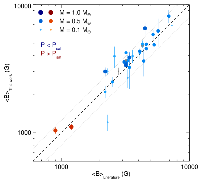
Figure 2: Comparison of our average field measurements to literature values. Red and blue symbols indicate slow and fast rotators, respectively (see Sect. 4.3), and gray symbols show stars with no information on rotation period. Symbol size and brightness indicate stellar mass. The dashed black line shows identity between our measurements and literature values, and the gray dotted lines mark the region where the discrepancy is within $\pm\,25$ %.

For many of our target stars, Moutou et al. (2017) reported average magnetic field measurements from an “indirect” method (Kochukhov, 2021). We provide a comparison between their results and our values in Appendix A.

4 Results

In this section, we investigate relations between average magnetic fields, rotation, and nonthermal emission. We augment our sample with stars for which average magnetic field measurements have been reported in the literature.

4.1 Sample

Figure 3: Distributions of our sample of stars with average magnetic field measurements. Left: Stellar mass. Center: Rotational period. Right: Rossby number. Rotational periods are known for 162 of the 314 sample stars, and the remaining 152 stars do not appear in the distributions of $P$ and $Ro$.

Our sample on Sun-like and low-mass stars consists of our measurements of 292 M dwarfs observed with CARMENES and 22 additional stars taken from the literature. From our original sample, we excluded those that did not meet the quality criteria for the selection of lines as described in Section 3. From the literature, we added only magnetic field measurements from radiative transfer calculations in multiple lines and considering multiple magnetic field components; following Kochukhov (2021), we added six M dwarfs from Shulyak et al. (2017). We also included the results on 15 young Sun-like stars from Kochukhov et al. (2020) and the value for the Sun from Trujillo Bueno et al. (2004).

The parameters for all 314 stars of our sample are listed in Table B.1. For the CARMENES stars, mass, radius, and luminosity are taken from Schweitzer et al. (2019). These values are derived from PARSEC isochrones and PHOENIX-ACES model fits to the high-resolution spectra (see Passegger et al., 2018). X-ray luminosities are computed from X-ray fluxes from Voges et al. (1999) using distances from Gaia Collaboration et al. (2021). Normalized H$\alpha$ luminosities are from CARMENES data (see Schöfer et al. (2019)). They are only reported for the stars with H$\alpha$ in emission. Ca H&K luminosities are estimated from normalized Ca emission $R^{\prime}_{\textrm{HK}}$ in Perdelwitz et al. (2021), we use $L_{\textrm{Ca}}=R^{\prime}_{\textrm{HK}}L_{\textrm{bol}}$. The main sources for uncertainties in X-ray, H$\alpha$, and Ca H&K luminosities are variability of the emission and uncertainties in the stellar parameters used to compute the luminosities from line equivalent widths. Variability and uncertainties are typically on the order of a few tenths of a dex (see, e.g., Schöfer et al., 2019; Perdelwitz et al., 2021). References for rotation periods are included in Table B.1. We discarded several periods measured by Díez Alonso et al. (2019) following a reanalysis of the same photometric data as used in that work but using more conservative thresholds for significance. As discussed in the references, it cannot be excluded that a few of the periods are false positives or harmonics of the real rotation periods. Obvious suspects could potentially be identified in cases where reported periods are in strong disagreement with the average relations between rotation and other information. For the young Suns from Kochukhov et al. (2020), we collected literature values for mass and radius from Takeda et al. (2007) and Chandler et al. (2016). We estimate the Rossby number, $Ro=P/\tau$, with $\tau=12.3$ d $\times\left(L_{\textrm{bol}}/L_{\odot}\right)^{-1/2}$, with rotation period, $P$, in days and bolometric luminosity, $L_{\textrm{bol}}$. The expression for $\tau$ was taken from Eq. (10) in Reiners et al. (2014), $P_{\textrm{sat}}=1.6\,\textrm{d}\times\left(L_{\textrm{bol}}/L_{\odot}\right)^{-1/2}$, and $\tau=P_{\textrm{sat}}/Ro_{\textrm{sat}}$. We use $Ro_{\textrm{sat}}=0.13$ for the transition between saturated and non-saturated activity (see Wright et al., 2011, 2018; Reiners et al., 2014). We note that Wright et al. (2018) derived a relationship $\tau(M)$ from X-ray observations in partially and fully convective stars that results in a similar scaling as the one we use here, but that yields smaller values of $\tau$ particularly for very low stellar mass. We confirmed that the main results of our analysis remain valid for $\tau(M)$ as expressed in Wright et al. (2018), and we emphasize that the relations we report in the following are independent of the choice of $\tau$.

The distribution of mass, $M$, rotation period, $P$, and Rossby number are shown in Fig. 3. The sample covers one order of magnitude in stellar mass with a concentration in the mass range $M$ = 0.4–0.5 M_⊙. The original motivation for the CARMENES survey was to search for planets around low-mass stars; our sample of magnetic field measurements therefore underrepresents stars more massive than 0.5 M_⊙. Most of the stars from Kochukhov et al. (2020) have masses close to the solar value. The sample covers three orders of magnitude in $P$ and $Ro$ with a strong concentration around $Ro=0.6$; 51 stars (16 %) of the sample are in the $0.5<Ro<0.8$ ($\log{g}\approx-0.2$) range. Although our sample mainly consists of stars that were observed to discover exoplanets, it was not intentionally biased towards slowly rotating or inactive stars. The rotational distribution of the sample is therefore a fair, albeit certainly not unbiased, representation of the (non-binary) stars in the local Galaxy. The distribution implies systematic biases and needs to be taken into account for what follows. The same applies for potential harmonics in the rotational periods, although their impact is probably small because of the large range in periods covered by our sample.

4.2 Period-mass diagram

Figure 4: Period-mass diagram indicating magnetic field strength in color and symbol size. Data from this work are shown as circles, and other data are shown as squares. Literature values are from Kochukhov et al. (2020) for young Sun-like stars and for seven additional targets from Shulyak et al. (2017). The solar datum from Trujillo Bueno et al. (2004) is annotated. Gray open circles show stars with known rotation periods as reported by Newton et al. (2017). Dashed lines show values of the Rossby number $Ro=0.1$ and 1.0, assuming that bolometric luminosity $L_{\textrm{bol}}\propto M^{4}$ and $\tau\propto L_{\textrm{bol}}^{-0.5}$ for dwarf stars.

The evolution in time of stellar rotation as a function of mass can be followed in a period-mass diagram (e.g., Barnes, 2003; Irwin et al., 2011; Reinhold et al., 2013; McQuillan et al., 2014). Observations of star clusters and field stars show the rotational evolution of stars from rapid rotators with very short rotational periods ($P<1$ d) to slower rotators with periods of $P=10$ d and longer depending on stellar mass. Stars are believed to lose angular momentum through the interaction between stellar wind and magnetic fields (e.g., Mestel, 1968; Kraft, 1970; Skumanich, 1972; Pallavicini et al., 1981; Kawaler, 1988; Reiners & Mohanty, 2012; Matt et al., 2015; Gallet & Bouvier, 2015; Vidotto, 2021).

Observations of nonthermal energy have shown that stellar activity is intimately coupled with rotation (Noyes et al., 1984; Pizzolato et al., 2003; Wright et al., 2011, 2018), and that the timescales for angular momentum loss and activity reduction depend on stellar mass (West et al., 2008). Stellar magnetic fields are the physical connection between nonthermal emission and rotational evolution. With our large set of magnetic field observations we can investigate this relation in detail and across a large parameter range. In Fig. 4, we show the distribution of our sample stars in the period-mass diagram and indicate the magnetic field strength. We include the stars with measured rotational periods from Newton et al. (2017) to show the distribution of available field measurements in context of a larger sample. We confirm that the two samples appear very similar in the mass-period diagram, and we refer the reader to Newton et al. (2017) for a discussion of this distribution in the context of stellar activity and rotational braking.

Figure 4 can be compared to diagrams visualizing the basic properties of the large-scale magnetic topologies of cool stars from ZDI, for example, in Donati & Landstreet (2009, Fig. 3,) and Kochukhov (2021, Fig. 14). A remarkable feature of such diagrams is a lack of stars at low masses ($M\la 0.3$ M_⊙) and rotation periods around 10 d and longer (or $Ro\ga 0.1$). This can partly be explained by a detection bias: small and slowly rotating stars have low Doppler broadening below the threshold values for ZDI. A low density of stars is also visible in Fig. 4 for masses below 0.3 $M_{\odot}$ in the period range around 10–40 d. However, stars with rotation periods around $P=100$ d do appear in this mass range. There is no obvious reason why rotation periods of several tens of days should be more difficult to detect than longer ones. Potential explanations for the low density of stars in this parameter range include enhanced braking efficiency in the relevant period range (see, e.g., Newton et al., 2016) and therefore rapid evolution of low-mass stars from a few days to about 100 d (similarly to attempts to explain the so-called Vaughan-Preston gap; Rutten, 1987), as well as cancellation of contrast features caused by a transition from dark to bright surface features (see, e.g., Reinhold et al., 2019). The distribution of magnetic fields in the period-mass diagram shows no peculiar features beyond a mass-dependent weakening of average magnetic fields with slower rotation. This is discussed in the following subsection.

4.3 Rotation-magnetic field relation

Figure 5: Magnetic field-rotation relation for solar-like and low-mass stars. Symbols for stars rotating slower than $Ro=0.13$ are colored red, while those of faster rotators are colored blue. Larger and darker symbols indicate higher stellar mass than smaller and lighter symbols. The gray dashed lines show linear fits separately for the slowly rotating stars ($Ro>0.13$; $\langle B\rangle=200$ G $\times\,Ro^{-1.25}$) and the fast rotators ($Ro<0.13$; $\langle B\rangle=2050$ G $\times\,Ro^{-0.11}$). Downward open triangles show upper limits for $\langle B\rangle$.

The decay of average magnetic field strength with rotation coincides with the well-studied dependence of stellar activity on rotation, as observed in nonthermal emission. The distribution of magnetic fields in Fig. 4 suggests a monotonous relation between rotation and average magnetic field, which is similar to the rotation-activity relation. The latter is often expressed as a dependence between normalized chromospheric or coronal emission from active regions ($L_{\textrm{activity}}/L_{\textrm{bol}}$) and the Rossby number. In Fig. 5, we show a similar relation between the average magnetic field $\langle B\rangle$ and Rossby number.

Our sample reveals a clear dependence between average magnetic field and Rossby number over more than three orders of magnitude in $Ro$. Similarly to the rotation-activity relation, the rotation-magnetic field relation exhibits a break between slow and rapid rotators, the saturated and the non-saturated groups of stars. The non-saturated group have Rossby numbers above $Ro=0.13$ (shown as red symbols in Fig. 5 and the following figures). In this group, the average magnetic field strongly depends on $Ro$. In the saturated group (blue symbols), the average field strength shows a much weaker dependence on rotation. The rotation-magnetic field relation of the saturated group was already apparent in Fig. 3 of Shulyak et al. (2017) and Fig. 12 of Kochukhov (2021).

Table 2: Relations between average magnetic field strength, $\langle B\rangle$ (in G), and Rossby number, Ro, and between magnetic flux, $\Phi_{\rm B}$ (in Mx) for the slow rotators (and the ratio $\langle B\rangle/B_{\rm kin}$ for the fast rotators), and rotation period, $P$ (in d).

Slow rotation ($Ro>0.13)$
$\langle B\rangle\,=199\,{\rm G}\times Ro^{-1.26\pm 0.10}$
$\Phi_{\rm B}=5.21\,10^{26}\,{\rm Mx}\times P^{-1.25\pm 0.07}$
Fast rotation ($Ro<0.13)$
$\langle B\rangle\,=2050\,{\rm G}\times Ro^{-0.11\pm 0.03}$
$\frac{\langle B\rangle}{B_{\rm kin}}=1.11\times P^{-0.16\pm 0.04}$

In order to quantify the relation between average magnetic field and Rossby number, we calculated linear regression curves following the ordinary least-squares (OLS) bisector method from Isobe et al. (1990). We chose the bisector method because the values of $Ro$ come with a relatively large uncertainty introduced by large systematic uncertainties in the convective turnover time, $\tau$. Coefficients of the relation are reported in Table 2. Additionally, our data suggest the existence of two branches for very slow rotation at $Ro\approx 1$. Stars rotating slower than this limit ($Ro>1$) are predominantly partially convective stars (see Fig. 4). Among them, some of the more massive stars’ field strengths seem to depend less on $Ro$ than the overall trend, but this speculation rests on very few data points only.

An alternative view on the rotation-activity relation is the scaling of chromospheric or coronal emission (non-normalized instead of normalized) with rotation period (instead of Rossby number). Such a scaling was suggested by Pallavicini et al. (1981), and Pizzolato et al. (2003) pointed out that the convective turnover time approximately scales as $\tau\propto L_{\textrm{bol}}^{-1/2}$. This parameterization is in general agreement with theoretical predictions (Kim & Demarque, 1996), but it is not obvious to what extent this justifies conclusions about the nature of the dynamo because $\tau$ likely depends on other parameters as well. Furthermore, the relevant $\tau$ may exhibit a discontinuity at the fully convective boundary (Cranmer & Saar, 2011), although so far no evidence for such a discontinuity was found (Wright et al., 2018). The scaling of $\tau$ with $L_{\textrm{bol}}$ implies that a relation between normalized emission ($L_{\textrm{activity}}/L_{\textrm{bol}}$) and Rossby number ($P/\tau$) is equivalent to a relation between $L_{\textrm{activity}}$ and rotation period. Furthermore, saturation of activity at a fixed Rossby number is equivalent to saturation at a fixed value of $L_{\textrm{activity}}/L_{\textrm{bol}}$ (see Reiners et al., 2014).

Figure 6: Alternative version of the rotation-magnetic field relation. Top panel: Ratio of average field, $\langle B\rangle$, to kinetic field limit, $B_{\textrm{kin}}$, as function of rotation period. Stars rotating faster than the saturation period are colored blue, while other stars are shown in gray. Bottom panel: Magnetic flux, $\Phi_{\textrm{B}}$. Stars rotating slower than the saturation limit are colored red, while faster rotators are shown in gray. Symbols and colors are the same as in Fig. 5. See text for details about $B_{\textrm{kin}}$.

We investigated scaling laws equivalent to the relation between average magnetic field and Rossby number (Fig. 5) and show an alternative view on the rotation-magnetic field relation in Fig. 6. In its upper panel, we show the ratio between the average magnetic field, $\langle B\rangle$, and the kinetic field strength limit (Reiners et al., 2009b),

$$B_{\textrm{kin}}=4800\,\textrm{G}\times\left(\frac{ML^{2}}{R^{7}}\right)^{1/6},$$ (1)

with $M$ being the stellar mass, $L$ luminosity, and $R$ radius, all in solar units. This expression estimates the maximum field strength under the hypothesis that energy flux determines the magnetic field strength in rapidly rotating stars (Christensen et al., 2009). We find that the observed average field strengths in the rapid rotators indeed populate a relatively narrow region with values $\langle B\rangle\approx B_{\textrm{kin}}$. We also find that the ratio $\langle B\rangle/B_{\textrm{kin}}$ shows a mild dependence on rotation with a power law coefficient that is significantly different from zero (see Table 2). Stars rotating slower than the saturation limit (gray symbols in the upper panel of Fig. 6) fall short of this relation. For these non-saturated stars, however, their magnetic flux, $\Phi_{\textrm{B}}=4\pi R^{2}B$, follows a relatively close relation with rotation period, as is shown in the lower panel of Fig. 6.

In the non-saturated stars of our sample, magnetic flux shows a clear dependence on rotational period. We report the relation between $\Phi_{\textrm{B}}$ and $P$ in Table 2 and indicate the relation as a dashed line in the lower panel of Fig. 6. A group of stars at $P<6$ d shows a somewhat different behavior, with values of $\Phi_{\textrm{B}}$ significantly below the overall trend. The group consists of relatively massive stars from the young Sun sample that may indicate an additional mass- or age-dependence, or that may be caused by a systematic offset in the literature values. We chose to not include stars with $M>0.9$ M_⊙ and $P<6$ d in our fit (seven stars). Potential reasons for this deviation from the trend defined by the lower mass stars include underestimated radii of the young stars (note that $\Phi_{\textrm{B}}\propto R^{2}$), an additional dependence of $\Phi_{\textrm{B}}$ on radius, age, or other parameters, and selection effects in our sample. We note that for the slow rotators, our relation between $\langle B\rangle$ and $Ro$ and the one between $\Phi_{\textrm{B}}$ and $P$ are conceptually equivalent because from the equations in Table 2, we estimate $\langle B\rangle\propto R^{-2}\propto\tau^{1.26}$, and hence $\tau\propto R^{-1.6}$. For main-sequence stars, this yields approximately $\tau\propto L^{-0.4}$, which is consistent with the scaling we assumed between $\tau$ and $L,$ as discussed above.

4.4 Predictive relations

Figure 7: Values for predicted value of average magnetic field calculated from Eqs. 2 and 3 valid for all masses. The dashed gray line indicates identity between $\langle B\rangle$ and $B_{\textrm{pred}}$, and the histogram shows the distribution of $\langle B\rangle$ around $B_{\textrm{pred}}$. We derive from the histogram that our relation estimates the value for $\langle B\rangle$ within roughly a factor of two uncertainty; this range is indicated with the two dotted lines.

Our results allow us to predict stellar magnetic fields from fundamental stellar parameters and rotational period, and therefore provide a missing link for physically consistent models of nonthermal emission (Linsky, 2017), cool star mass loss (Cranmer & Saar, 2011), and angular momentum evolution (Gallet & Bouvier, 2015). One of our main results is that the average magnetic field of a main-sequence star with $M\la 1$ M_⊙, generated by the magnetic dynamo, can be approximated from stellar parameters mass, $M$, radius, $R$, luminosity, $L$, (all in solar units), and rotation period, $P$, (in days) in the following way:

$$B_{\textrm{pred}}= 8570\,{\rm G}\times R^{-2}\times P^{-1.25}\quad(\textrm{slow rotation;}\,P>P_{\textrm{sat}}),$$ (2)

$$B_{\textrm{pred}}= 5300\,{\rm G}\times\left(\frac{ML^{2}}{R^{7}}\right)^{\frac{1}{6}}\times P^{-0.16}\quad(\textrm{fast rotation;}\,P<P_{\textrm{sat}}).$$ (3)

Equation (2) follows from the relations between $\Phi_{B}$ and $P$ for the slow rotators in Table 2 and is independent of the choice of $\tau$. Equation (3) follows from the relation between $\langle B\rangle/B_{\textrm{kin}}$ and $P$ for the fast rotators together with Eq. (1). The critical period can be estimated as $P_{\textrm{sat}}=1.6\,\textrm{d}\times\left(L_{\textrm{bol}}/L_{\odot}\right)^{-1/2}$, which corresponds to $Ro=0.13$. In Fig. 7, we show the measured average fields in relation to the predicted values. In the histogram, we show the distribution of the ratio $\langle B\rangle/B_{\textrm{pred}}$. We find that 75 % of the predicted values agree with the measured values within a factor of two.

4.5 Nonthermal emission

The magnetic field-rotation relation (Fig. 5) shows remarkable similarity to the activity-rotation relation from X-ray emission. Other frequently used indicators of stellar activity include the hydrogen H$\alpha$ line of the Balmer series and the Ca H&K lines. X-rays are emitted at temperatures occurring in the stellar coronae, while both H$\alpha$ and Ca H&K form at lower temperatures in the chromosphere (Vernazza et al., 1981). A relation between photospheric magnetic flux, $\Phi_{\textrm{B}}$, and X-ray spectral luminosity, $L_{\textrm{X}}$, was established by Pevtsov et al. (2003) that applies to X-ray irradiance from bright stellar surface regions as well as the total stellar X-ray output. Such a relation constrains possible heating and emission models for the Sun and other stars (Fontenla et al., 2016).

Figure 8: Normalized coronal (X-ray, top panel) and chromospheric (H$\alpha$, middle panel; Ca H&K, bottom panel) emission as a function of average magnetic field. Symbol size and color are the same as in Fig. 5. The arrow in the bottom panel indicates the field strength at which the normalized Ca H&K emission saturates.

Before we turn to the emission/magnetic flux relation, we investigated the dependence between normalized line luminosity ($L_{\textrm{(X, H}\alpha\textrm{, Ca)}}/L_{\textrm{bol}}$) and average magnetic field in Fig. 8. These relations show a relatively large scatter but provide information about the typical field strengths required to generate observable chromospheric and coronal emission. We find that X-ray and Ca H&K emission are observable in stars with very low magnetic field strengths, which possibly includes a basal component that is unrelated to stellar magnetic activity (Schrijver et al., 1989). On the other hand, we find that a minimum average field strength of several hundred G is required in order to generate detectable H$\alpha$ emission in a stellar chromosphere. This is consistent with chromosphere models in low-mass stars, showing that Balmer line emission is only generated in the presence of a sufficiently massive chromosphere (Cram & Mullan, 1979). For Ca H&K, we observe a saturation of the normalized emission at a magnetic field strength $\langle B\rangle\ga 800$ G, that is, an increase in the average magnetic field beyond 800 G does not lead to an obvious increase in $L_{\textrm{Ca}}/L_{\textrm{bol}}$.

Figure 9: Coronal ($L_{\textrm{X}}$, top panel) and chromospheric ($L_{\textrm{H}\alpha}$, middle panel; $L_{\textrm{Ca}}$, bottom panel) emission luminosities as a function of magnetic flux, $\Phi_{\textrm{B}}$. Symbol size and color are the same as in Fig. 5. Linear power laws are reasonable approximations for X-ray, H$\alpha$, and Ca luminosities describing both rapid and slow rotators. Relations are provided in Eqs. 4–6. Ca H&K emission shows a saturation at magnetic flux density $\langle B\rangle\approx 800$ G (see Fig. 8). This limit is applied to the magnetic flux values in the bottom panel (Ca H&K), but no limit is applied in the other two panels.

In Fig. 9, we show that well-defined relations exist between magnetic flux and emission luminosities in all three stellar activity indicators, that is, X-rays, hydrogen H$\alpha$, and Ca H&K. These relations show significantly less scatter than those between normalized activity and average magnetic field in Fig. 8. Ca H&K and X-ray emission are already visible at magnetic flux levels below $\Phi_{\textrm{B}}=10^{24}$ Mx. H$\alpha$ emission requires more magnetic heating and goes together with relatively strong Ca H&K emission (Robinson et al., 1990). For the plot showing Ca H&K emission (bottom panel in Fig. 9), we applied a saturation limit of $B_{\textrm{max}}=800$ G in the calculation of magnetic flux because higher average fields show no increase in normalized emission for stronger fields (see above); for all stars with $\langle B\rangle>800$ G, we set $\langle B\rangle=800$ G when calculating $\Phi_{\textrm{B}}$. We interpret this as saturation of chromospheric Ca H&K emission at a field strength of $\sim$800 G. We note that the choice of higher maximum field strengths would essentially shift the blue points (rapid rotators) in the bottom panel of Fig. 9 toward the right; a limit of 1000 G instead of 800 G already moves the blue points significantly away from the relation.

We summarize relations between chromospheric and coronal emission and magnetic flux in Eqs. 4–6. The relations apply to all stars across the entire range of masses and rotation rates included in our sample (taking into account the field limit in Ca H&K). Our relations quantitatively describe the dependence of nonthermal chromospheric and coronal emission on the stellar dynamo. With luminosities, $L$, in erg s^-1 and magnetic flux, $\Phi_{\textrm{B}}$, in Mx, we can write:

$$L_{\textrm{X}}= 3.28\,10^{-12}\times\Phi_{\textrm{B}}^{1.58\pm 0.06}$$ (4)

$$L_{\textrm{H}\alpha}= 4.80\,10^{-9\phantom{1}}\times\Phi_{\textrm{B}}^{1.43\pm 0.05}$$ (5)

$$L_{\textrm{Ca}}= 1.22\,10^{-19}\times\Phi_{\textrm{B}}^{1.88\pm 0.05} (\textrm{apply}B_{\textrm{max}}=800\,\textrm{G}).$$ (6)

5 Summary and discussion

We provided direct measurements of average magnetic field strengths in 292 low-mass main-sequence stars from radiative transfer calculations considering multiple magnetic field components. For 260 stars of our sample, average field values are reported here for the first time. Our new data were collected as part of the CARMENES survey for planets around M dwarfs; in total, we used 15,058 spectra for our analysis, which were corrected for telluric contamination before co-addition.

The average field strengths we measured span approximately two orders of magnitude with a lower limit around 100 G and maximum values of 8000 G. Not surprisingly, we observe a relatively large scatter in our investigations of average field strengths, but a number of clear trends appear that allow us to draw firm conclusions about the role of average magnetic fields in the framework of stellar activity. For our analysis, we included literature data for 22 stars that were obtained with similar methods.

First, we find that the saturation-type, rotation-activity relation, which is well known from nonthermal coronal emission, can be traced back to a rotation-magnetic field relation between average field strength, rotation period, and fundamental stellar parameters. Our data show that rapid and slow rotators behave differently with a break around $Ro=0.13$, which is where the average surface field reaches the kinetic field strength limit. This demonstrates that a saturation effect in the magnetic dynamo is the reason for saturation of nonthermal emission instead of a limit in the available stellar surface area (filling factor equal to unity). We provided relations between magnetic flux ($\Phi_{\textrm{B}}=4\pi R^{2}B$) and rotation period valid for the non-saturated (slowly rotating) stars. From this relation, we derived a relationship between average magnetic field strength as a function of rotation period and stellar radius that is independent of the choice of the convective turnover time. As an equivalent description of the rotation-magnetic field relation, we also find a relationship between average magnetic field and Rossby number. We see some systematic deviations between our data and the predictions, which hints at additional effects that go beyond our scaling relations. Saturated (rapidly rotating) stars consistently show average field strengths close to the kinetic field strength limit; the ratio between average field strength and the kinetic limit is close to unity in the saturated stars but reveals a mild dependence on rotation.

Second, we investigated relations between nonthermal chromospheric and coronal emission from X-ray, H$\alpha$, and Ca H&K measurements. We observe that emission luminosity normalized by the stars’ bolometric luminosity is related to average field strengths. In addition, Ca H&K line emission shows saturation at an average field strength around 800 G. Taking this saturation into account provides close relations between X-ray, H$\alpha$, and Ca H&K luminosity with magnetic flux for all our sample stars. We reported relations between magnetic flux and emission luminosities for the three types of emission lines.

The universal correspondence between magnetic flux and nonthermal emission sheds some light on the proposed mechanism of centrifugal stripping, according to which that correspondence was suspected to break down in the most rapid rotators (Jeffries et al., 2011; Christian et al., 2011). Centrifugal stripping is consistent with the apparent reduction of flaring activity in very rapidly rotating M dwarfs with $P\la 0.3$ d (Günther et al., 2020; Ramsay et al., 2020). A potential mechanism is decreased effective gravity leading to distortion of magnetic field lines and cooling of the coronal plasma to chromospheric temperatures (Antiochos et al., 2011). An observational signature of this effect would be rapidly rotating stars with typical chromospheric but abnormally low coronal luminosities with respect to their magnetic flux. The observed correlation between X-ray emission and magnetic flux (Fig. 9) shows no evidence for supersaturation caused by a break in coronal heating. Instead, saturation of normalized emission with magnetic flux density is visible in the chromospheric Ca H&K lines (Fig. 8). Our results are therefore not consistent with the coronal stripping scenario.

Figure 10: Relation between magnetic energy and the ratio between kinetic energy and Rossby number for our sample stars. Such a relation is motivated by the assumption of a balance between Coriolis, buoyancy, and Lorentz forces (MAC balance). Symbols are the same as in Fig. 5.

Our data allow us to test the prediction from force balance (MAC balance) that magnetic energy grows in proportion to the ratio between kinetic energy and Rossby number, $E_{\textrm{B}}\sim E_{\textrm{kin}}/Ro$ (e.g., Brun & Browning, 2017). We show this relation for our sample stars in Fig. 10. A clear correlation is visible, but we can identify a few obvious trends that show systematic deviations from the simplified scaling law, for example, at $E_{\textrm{kin}}/Ro\approx 10^{39}$ erg; intermediate mass stars show values of $E_{\textrm{B}}$ that are about one order of magnitude larger than the highest or lowest mass stars in our sample. Our data set provides valuable input for more detailed tests of dynamo models that go beyond the scope of this paper.

Looking at all observations together, we conclude that the rotation-activity relation, including its saturation effect, is a causal consequence of the characteristics of the magnetic dynamo and its dependence on rotation. We promote the notion that the magnetic dynamo generates magnetic flux proportionally to the rotation rate with a limit defined by the available kinetic energy. Coronal and chromospheric emission are generated with total nonthermal emission proportionally to magnetic flux. Therefore, nonthermal emission scales with rotation period until the magnetic field saturation limit is reached, beyond which point the emission only mildly depends on rotation (because a mild dependence between magnetic flux and rotation still exists in the saturation regime). With this background, coronal and chromospheric emission can be estimated from stellar parameters according to Eqs. 2–6. For example, for coronal X-ray emission in non-saturated stars, we estimate that $L_{\textrm{X}}\propto\Phi_{\textrm{B}}^{1.58\pm 0.06}$ and $\Phi_{\textrm{B}}\propto P^{-1.25\pm 0.07}$, which implies $L_{\textrm{X}}\propto P^{-1.98\pm 0.07}$, which is consistent with the observed X-ray activity-rotation relation from much larger samples.

The new observations provide a direct view into magnetic dynamos of low-mass stars, and they yield a consistent picture of chromospheric and coronal emission for stars of different masses and rotation periods. The relations between fundamental stellar parameters, rotation, average magnetic fields, and nonthermal emission provide useful information for models of stellar and planetary evolution.

Appendix A Comparison to Moutou et al. (2017)

Figure 11: Comparison between average magnetic field measurements reported by Moutou et al. (2017) and our results. Lines, symbols and colors are the same as in Fig. 2.

Similarly to our literature comparison in Fig. 2, where we considered only analyses using multi-component radiative transfer and multiple lines, Fig. 11 shows a comparison between the results from Moutou et al. (2017) and our values, extending the comparison carried out by Kochukhov (2021, which is shown in their Fig. 11). Both sets of results show relatively little correlation. Most of the values from Moutou et al. (2017) scatter around $Bf=$ 1–2 kG, which includes stars where we measured significantly lower field strengths. A potentially systematic effect among the slow rotators was already suspected by Moutou et al. (2017).

Appendix B Star Table

1]

Table 3: Table with stellar parameters and results from our analysis

#	Karmn	Name	NObs	S/N	$M$	$R$	$T_{\rm eff}$	$P$	Ref. $P$	$\tau$	$\log{\frac{L_{\rm bol}}{L_{\odot}}}$	$\log\frac{L_{\rm X}}{L_{\rm bol}}$	$\log\frac{L_{\rm H\alpha}}{L_{\rm bol}}$	$\log\frac{L_{\rm Ca}}{L_{\rm bol}}$	$\langle B\rangle$	$\Delta\langle B\rangle$	$\varv\sin{i}$
				@8700 Å	(M⊙)	(R⊙)	(K)	(d)		(d)					(G)	(G)	(km s-1)
1	J02565+554W	Ross 364	10	270	0.61	0.61	3832	51.2	SM18	45	$-$1.14				380	80	0.3
2	J02573+765	G 245$-$61	54	300	0.24	0.25	3381			143	$-$2.13				$<$ 390		0.0
3	J03133+047	CD Cet	109	660	0.18	0.21	3214	126.2	New16a	226	$-$2.53			$-$5.22	250	90	0.0
4	J03181+382	HD 275122	44	820	0.60	0.60	3826	77.2	DA19	49	$-$1.20			$-$4.93	$<$ 360		1.4
5	J03213+799	GJ 133	24	480	0.44	0.43	3599	32.4	DA19	78	$-$1.61				320	110	0.0
6	J03217$-$066	G 77$-$046	11	310	0.49	0.48	3661	21.1	DA19	67	$-$1.48	$-$4.65		$-$4.52	930	110	1.4
7	J03463+262	HD 23453	48	780	0.60	0.60	3949			45	$-$1.14	$-$4.80		$-$4.40	470	60	1.7
8	J03473$-$019	G 80$-$021	11	280	0.50	0.50	3473	3.9	Rev20	69	$-$1.51	$-$3.04	$-$3.67	$-$3.97	3490	200	6.0
9	J03531+625	Ross 567	35	620	0.39	0.38	3501			94	$-$1.77				260	70	0.0
10	J04153$-$076	omi02 Eri C	53	580	0.25	0.26	3179			154	$-$2.20	$-$3.17	$-$3.94		3020	140	2.2
11	J04167$-$120	LP 714$-$47	35	270	0.59	0.58	3961			45	$-$1.13				650	140	2.2
12	J04219+213	LP 415$-$17	4	50	0.58	0.57	3940			46	$-$1.14				$<$ 500		0.0
13	J04225+105	LSPM J0422+1031	18	330	0.48	0.47	3546		(DA19)	78	$-$1.60			$-$5.14	190	70	0.0
14	J04290+219	BD+21 652	170	1490	0.62	0.85	4123	25.4	DA19	36	$-$0.94	$-$4.54		$-$4.44	380	60	1.3
15	J04311+589	STN 2051A	11	310	0.28	0.29	3382			125	$-$2.02	$-$4.65			$<$ 490		0.0
16	J04343+430	PM J04343+4302	56	320	0.47	0.46	3525			71	$-$1.52				$<$ 370		0.0
17	J04376+528	BD+52 857	126	1310	0.55	0.55	4039			46	$-$1.14	$-$4.77		$-$4.44	430	50	0.7
18	J04376$-$110	BD$-$11 916	22	540	0.49	0.48	3666			67	$-$1.48			$-$5.04	$<$ 430		0.0
19	J04429+189	HD 285968	23	450	0.51	0.51	3678	40.7	DA19	65	$-$1.46	$-$4.64		$-$4.74	350	80	0.0
20	J04429+214	2MASS J04425586+2128	10	280	0.42	0.42	3499	47.8	DA19	91	$-$1.74			$-$4.97	420	90	0.5
21	J04472+206	RX J0447.2+2038	11	150	0.38	0.39	3096	0.3	CC21	110	$-$1.90	$-$3.12	$-$3.53		6230	1540	45.4
22	J04520+064	Wolf 1539	10	270	0.40	0.40	3439			95	$-$1.78			$-$5.04	$<$ 410		0.0
23	J04538$-$177	GJ 180	24	560	0.43	0.42	3582			79	$-$1.62			$-$5.09	$<$ 420		0.0
24	J04588+498	BD+49 1280	55	910	0.62	0.62	3983			43	$-$1.10	$-$5.02		$-$4.43	460	40	1.9
25	J05019+011	1RXS J050156.7+01084	19	310	0.38	0.61	3217	2.1	Rev20	67	$-$1.47	$-$3.04	$-$3.57	$-$4.18	3320	250	7.0
26	J05019$-$069	LP 656$-$038	8	260	0.18	0.21	3284	88.5	Kira12	204	$-$2.44	$-$3.91	$-$4.57	$-$4.75	1140	350	1.7
27	J05033$-$173	LP 776$-$046	37	590	0.29	0.30	3464			127	$-$2.03			$-$5.26	270	70	0.0
28	J05062+046	RX J0506.2+0439	13	210	0.35	0.58	3134	0.9	Rev20	73	$-$1.55	$-$3.12	$-$3.52	$-$4.53	3070	490	29.0
29	J05127+196	GJ 192	25	530	0.46	0.45	3599			75	$-$1.57			$-$5.17	$<$ 380		0.0
30	J05280+096	Ross 41	17	330	0.26	0.27	3440		(DA19)	149	$-$2.17				$<$ 410		1.1
31	J05314$-$036	HD 36395	95	1210	0.54	0.54	3850	33.8	DA19	48	$-$1.19	$-$4.81		$-$4.53	210	50	2.1
32	J05348+138	Ross 46	15	440	0.39	0.39	3464			99	$-$1.81	$-$4.28		$-$5.19	340	60	0.0
33	J05360$-$076	Wolf 1457	24	370	0.37	0.37	3422			109	$-$1.90				$<$ 210		0.0
34	J05365+113	V2689 Ori	130	1420	0.63	0.63	4067	11.5	CC21	43	$-$1.10	$-$4.09	$-$4.53	$-$4.14	1110	60	2.0
35	J05366+112	2MASS J05363846+1117	14	350	0.30	0.31	3355			130	$-$2.05		$-$3.93	$-$4.16	2520	180	3.4
36	J05394+406	LSR J0539+4038	18	50	0.10	0.12	2600			517	$-$3.25		$-$4.52		1830	380	5.3
37	J05415+534	HD 233153	97	1180	0.58	0.58	3825			51	$-$1.24	$-$3.79		$-$4.44	420	60	1.9
38	J05421+124	V1352 Ori	51	730	0.26	0.27	3324			155	$-$2.20	$-$4.86		$-$5.51	$<$ 280		0.0
39	J06000+027	G 99$-$049	14	300	0.26	0.27	3296	1.8	Rev20	155	$-$2.20	$-$3.41	$-$3.95	$-$4.16	2490	220	6.2
40	J06011+595	G 192$-$013	80	910	0.30	0.30	3431			134	$-$2.08			$-$5.16	210	60	0.0
41	J06024+498	G 192$-$015	36	290	0.15	0.18	3213	105.0	DA19	269	$-$2.68				370	120	0.0
42	J06103+821	GJ 226	56	800	0.44	0.44	3554	44.6	DA19	79	$-$1.62	$-$5.04		$-$5.09	$<$ 200		0.0
43	J06105$-$218	HD 42581 A	50	760	0.54	0.55	3801	27.3	DA19	52	$-$1.26	$-$5.19		$-$4.64	380	70	0.5
44	J06246+234	Ross 64	6	180	0.18	0.20	3249			215	$-$2.48				620	140	0.0
45	J06318+414	LP 205$-$044	33	230	0.40	0.41	3084	0.3	Rev20	106	$-$1.87	$-$2.96	$-$3.52		2200	1150	54.0
46	J06371+175	HD 260655	55	850	0.48	0.48	3803			64	$-$1.44	$-$4.84		$-$4.84	190	40	0.0
47	J06396$-$210	LP 780$-$032	54	440	0.33	0.33	3428			105	$-$1.86	$-$4.20			620	110	1.6
48	J06421+035	G 108$-$021	19	450	0.41	0.40	3475	83.4	DA19	91	$-$1.74			$-$5.08	180	60	0.0
49	J06548+332	Wolf 294	255	1790	0.39	0.39	3503		(DA19)	96	$-$1.79	$-$5.66		$-$5.38	$<$ 290		0.0
50	J06574+740	2MASS J06572616+7405	13	230	0.27	0.28	3173			147	$-$2.15	$-$2.93	$-$3.64		3330	830	32.0
51	J06594+193	GJ 1093	27	270	0.14	0.17	3146			308	$-$2.80			$-$5.91	390	120	0.0
52	J07033+346	LP 255$-$011	14	300	0.28	0.29	3310	8.0	DA19	143	$-$2.13		$-$3.90		2430	160	2.4
53	J07044+682	GJ 258	16	370	0.43	0.42	3527			83	$-$1.66				$<$ 270		0.0
54	J07274+052	Luyten’s Star	242	1260	0.28	0.29	3380	93.5	SM17b	124	$-$2.01	$-$5.33		$-$5.27	$<$ 440		0.0
55	J07287$-$032	GJ 1097	20	460	0.37	0.37	3511			88	$-$1.72			$-$5.31	$<$ 310		0.0
56	J07319+362N	BL Lyn	38	670	0.43	0.43	3289	16.4	DA19	90	$-$1.73	$-$2.75	$-$3.93	$-$4.27	2530	140	1.7
57	J07353+548	GJ 3452	6	250	0.40	0.39	3564		(DA19)	89	$-$1.72				$<$ 250		0.0
58	J07386$-$212	LP 763$-$001	6	200	0.29	0.29	3488			115	$-$1.94			$-$5.29	$<$ 290		0.0
59	J07393+021	BD+02 1729	35	690	0.62	0.62	3980			44	$-$1.11			$-$4.53	280	50	1.7
60	J07403$-$174	LP 783$-$002	49	120	0.11	0.14	3031			425	$-$3.08	$-$4.13			280	170	0.0
61	J07446+035	YZ CMi	51	650	0.33	0.33	3251	2.8	Rev20	116	$-$1.95	$-$2.98	$-$3.61		4540	150	4.6
62	J07472+503	2MASS J07471385+5020	15	290	0.29	0.29	3251	1.3	Rev20	138	$-$2.10	$-$3.76	$-$3.80		2940	290	10.3
63	J07558+833	GJ 1101	14	230	0.28	0.29	3252	1.1	Rev20	142	$-$2.13	$-$3.03	$-$3.75		3610	480	11.8
64	J07582+413	GJ 1105	27	480	0.30	0.31	3431			131	$-$2.06			$-$5.33	$<$ 240		0.0
65	J08023+033	G 50$-$16 A	67	310	0.34	0.35	3422			100	$-$1.82				260	150	0.0
66	J08119+087	Ross 619	16	340	0.16	0.18	3245		(DA19)	240	$-$2.58				920	90	0.4
67	J08126$-$215	GJ 300	18	370	0.30	0.31	3356			134	$-$2.07	$-$4.96		$-$5.05	$<$ 400		0.0
68	J08161+013	GJ 2066	56	830	0.44	0.44	3570	40.7	DA19	73	$-$1.55			$-$5.00	250	40	0.0
69	J08293+039	2MASS J08292191+0355	14	440	0.50	0.50	3651			65	$-$1.45			$-$4.51	410	80	0.8
70	J08298+267	DX Cnc	31	360	0.09	0.11	2997	0.5	DA19	426	$-$3.08		$-$4.31		2680	440	11.5
71	J08315+730	LP 035$-$219	19	300	0.31	0.31	3364	105.0	DA19	127	$-$2.03				$<$ 450		0.0
72	J08358+680	G 234$-$037	11	300	0.40	0.39	3496			92	$-$1.75	$-$4.48			580	80	1.1
73	J08402+314	LSPM J0840+3127	7	280	0.32	0.32	3426	118.0	DA19	123	$-$2.00				310	90	0.0
74	J08409$-$234	LP 844$-$008	23	370	0.40	0.40	3496			83	$-$1.66			$-$5.02	$<$ 510		0.0
75	J08413+594	LP 090$-$018	177	420	0.13	0.16	3141			299	$-$2.77		$-$4.44		1280	210	2.0
76	J08526+283	rho Cnc B	11	260	0.30	0.31	3321			138	$-$2.10			$-$5.08	$<$ 590		0.0
77	J08536$-$034	LP 666$-$009	42	30	0.08	0.10	2400	0.5	Rev20	735	$-$3.55	$-$3.37	$-$3.93		4790	470	8.4
78	J09003+218	LP 368$-$128	21	140	0.08	0.10	3061	0.4	New16a	437	$-$3.10	$-$3.41	$-$4.15		4270	370	13.0
79	J09028+680	LP 060$-$179	10	280	0.30	0.30	3328			134	$-$2.08				$<$ 450		0.0
80	J09033+056	NLTT 20861	29	80	0.14	0.15	3027			289	$-$2.74		$-$4.46		3220	480	7.1
81	J09143+526	HD 79210	70	770	0.58	0.57	4015			44	$-$1.12	$-$4.22		$-$4.46	400	50	1.0
82	J09144+526	HD 79211	158	1400	0.61	0.61	3983			44	$-$1.12	$-$4.69		$-$4.47	340	40	0.5
83	J09161+018	RX J0916.1+0153	9	200	0.33	0.33	3237	1.4	Rev20	122	$-$1.99	$-$3.28	$-$3.68	$-$3.77	3900	360	10.0
84	J09163$-$186	LP 787$-$052	5	250	0.48	0.48	3697			67	$-$1.48	$-$4.31	$-$4.65	$-$4.53	740	150	1.0
85	J09307+003	GJ 1125	21	470	0.34	0.34	3460			114	$-$1.93			$-$5.36	180	50	0.0
86	J09360$-$216	GJ 357	25	610	0.37	0.36	3496	74.3	SM15	97	$-$1.79			$-$5.44	$<$ 260		0.0
87	J09411+132	Ross 85	24	570	0.49	0.49	3699			66	$-$1.47	$-$4.55		$-$4.76	390	70	0.0
88	J09423+559	GJ 363	10	280	0.41	0.41	3439	74.3	DA19	93	$-$1.76				320	80	0.0
89	J09425+700	GJ 360	35	610	0.52	0.52	3547	21.0	DA19	66	$-$1.46	$-$4.18	$-$4.47		1030	110	2.1
90	J09428+700	GJ 362	24	540	0.46	0.46	3504	23.9	DA19	79	$-$1.62	$-$3.69	$-$4.40	$-$4.49	1390	140	1.1
91	J09439+269	Ross 93	4	200	0.42	0.41	3492		(DA19)	91	$-$1.75			$-$5.27	$<$ 500		0.5
92	J09447$-$182	GJ 1129	12	300	0.32	0.32	3417			127	$-$2.03			$-$5.28	$<$ 310		0.0
93	J09449$-$123	G 161$-$071	10	180	0.33	0.34	3068	0.4	Rev20	130	$-$2.05	$-$2.90	$-$3.38		4860	990	35.3
94	J09468+760	BD+76 3952	20	510	0.52	0.51	3616			59	$-$1.37				$<$ 410		0.0
95	J09511$-$123	BD$-$11 2741	18	520	0.53	0.53	3769			57	$-$1.33			$-$4.93	150	50	0.0
96	J09561+627	BD+63 869	69	920	0.60	0.60	3938			45	$-$1.14	$-$4.81		$-$4.44	390	50	1.9
97	J10023+480	BD+48 1829	21	510	0.58	0.59	3739			50	$-$1.22				200	60	0.1
98	J10088+692	TYC 4384$-$1735$-$1	41	500	0.64	0.63	3952			41	$-$1.06				210	50	0.0
99	J10122$-$037	AN Sex	76	960	0.52	0.52	3720	21.6	DA19	60	$-$1.38	$-$4.86		$-$4.56	450	80	1.5
100	J10125+570	LP 092$-$048	7	290	0.33	0.33	3474			113	$-$1.93			$-$5.26	240	80	0.0
101	J10167$-$119	GJ 386	12	390	0.50	0.50	3552			68	$-$1.49			$-$5.06	$<$ 200		0.1
102	J10185$-$117	LP 729$-$054	51	410	0.37	0.37	3434			93	$-$1.76				$<$ 280		0.0
103	J10196+198	AD Leo	46	500	0.42	0.42	3477	2.2	Mori08	80	$-$1.63	$-$3.08	$-$3.64		3570	90	3.3
104	J10251$-$102	BD$-$09 3070	21	550	0.51	0.51	3759			57	$-$1.33	$-$5.09		$-$4.60	380	50	1.1
105	J10289+008	BD+01 2447	85	1020	0.45	0.45	3588	32.7	CC21	76	$-$1.59	$-$5.17		$-$4.91	270	60	0.0
106	J10350$-$094	LP 670$-$017	16	360	0.42	0.41	3512			87	$-$1.71			$-$5.15	$<$ 520		0.0
107	J10360+051	RY Sex	7	210	0.36	0.36	3268			105	$-$1.87	$-$3.12	$-$3.64		4820	140	2.1
108	J10396$-$069	GJ 399	7	280	0.49	0.49	3592			69	$-$1.50			$-$5.02	$<$ 560		0.0
109	J10416+376	GJ 1134	7	200	0.24	0.26	3298	54.3	DA19	170	$-$2.28				$<$ 820		0.0
110	J10508+068	EE Leo	48	760	0.29	0.30	3410	64.0	DA19	138	$-$2.10			$-$5.10	$<$ 400		0.0
111	J10564+070	CN Leo	78	670	0.09	0.11	3071	2.7	DA19	387	$-$3.00	$-$3.54	$-$3.98		3010	160	0.0
112	J10584$-$107	LP 731$-$076	53	250	0.19	0.21	3218			192	$-$2.39	$-$3.30	$-$3.85		4100	170	2.8
113	J11000+228	Ross 104	60	810	0.42	0.42	3532			88	$-$1.71	$-$4.93		$-$5.10	360	60	0.0
114	J11026+219	DS Leo	53	820	0.57	0.57	3846	13.5	CC21	51	$-$1.25	$-$3.94	$-$4.53	$-$4.12	1040	60	2.3
115	J11033+359	Lalande 21185	379	2320	0.42	0.41	3557	48.0	KS07	82	$-$1.65	$-$5.23		$-$5.46	$<$ 200		0.0
116	J11054+435	BD+44 2051A	111	1180	0.38	0.38	3628	100.9	SM18	81	$-$1.64	$-$5.32		$-$5.46	$<$ 200		0.0
117	J11055+435	WX UMa	37	340	0.08	0.10	3278	0.8	Mori10	398	$-$3.02	$-$3.15	$-$3.56		6880	140	3.5
118	J11110+304E	HD 97101	13	470	0.67	0.66	4211	38.5	Oel18	35	$-$0.91				$<$ 330		2.0
119	J11110+304W	HD 97101 B	49	750	0.55	0.54	3730			54	$-$1.29	$-$5.10		$-$4.78	280	70	0.7
120	J11126+189	StKM 1$-$928	20	540	0.51	0.51	3752			57	$-$1.34			$-$4.59	300	50	0.4
121	J11201$-$104	LP 733$-$099	27	520	0.53	0.53	3697	5.6	Rev20	60	$-$1.38	$-$3.21	$-$3.94		2170	160	4.6
122	J11302+076	K2$-$18	63	310	0.47	0.46	3563	38.8	CC21	74	$-$1.56			$-$4.97	270	80	0.1
123	J11306$-$080	LP 672$-$042	14	350	0.39	0.39	3486			97	$-$1.80				380	90	0.0
124	J11417+427	Ross 1003	80	930	0.40	0.40	3387	71.5	DA19	101	$-$1.83			$-$5.34	$<$ 240		0.0
125	J11421+267	Ross 905	440	1020	0.46	0.45	3533	44.6	DA19	79	$-$1.62	$-$5.18		$-$5.27	$<$ 200		0.0
126	J11467$-$140	GJ 443	15	390	0.52	0.52	3565			64	$-$1.44			$-$4.77	270	80	0.9
127	J11474+667	1RXS J114728.8+66440	40	200	0.28	0.29	3219	13.4	CC21	137	$-$2.09	$-$3.67	$-$3.70		4770	140	3.1
128	J11476+002	LP 613$-$049 A	6	140	0.34	0.34	3282	11.6	DA19	111	$-$1.91	$-$3.14	$-$3.68	$-$4.08	3720	180	2.3
129	J11476+786	GJ 445	64	770	0.28	0.29	3361			137	$-$2.10	$-$4.85		$-$5.61	$<$ 320		0.0
130	J11477+008	FI Vir	56	720	0.20	0.22	3325	163.0	DA19	198	$-$2.41	$-$4.32		$-$5.21	280	110	0.0
131	J11509+483	GJ 1151	65	510	0.19	0.21	3282	125.0	DA19	214	$-$2.48				$<$ 680		0.0
132	J11511+352	BD+36 2219	110	1150	0.49	0.48	3692	22.8	DA19	67	$-$1.48	$-$4.44		$-$4.62	660	60	0.0
133	J12100$-$150	LP 734$-$032	47	610	0.41	0.41	3415			97	$-$1.80			$-$5.19	$<$ 320		0.0
134	J12111$-$199	LTT 4562	19	410	0.39	0.38	3517			95	$-$1.77			$-$5.19	$<$ 420		0.0
135	J12123+544S	HD 238090	110	1240	0.58	0.58	3902			46	$-$1.15				210	40	0.0
136	J12156+526	StKM 2$-$809	13	250	0.53	0.53	3360	0.7	Rev20	67	$-$1.48	$-$2.98	$-$3.64		6530	680	37.6
137	J12189+111	GL Vir	13	230	0.15	0.18	3064	0.5	DA19	270	$-$2.68	$-$3.25	$-$3.76	$-$4.70	3970	460	13.0
138	J12230+640	Ross 690	149	880	0.51	0.50	3563	32.9	DA19	66	$-$1.47			$-$5.06	$<$ 220		1.1
139	J12248$-$182	Ross 695	15	390	0.28	0.29	3432			124	$-$2.01			$-$5.42	290	70	1.1
140	J12312+086	BD+09 2636	48	800	0.57	0.57	3896			49	$-$1.20			$-$4.51	360	40	1.0
141	J12373$-$208	LP 795$-$038	18	190	0.45	0.45	3431			87	$-$1.70			$-$5.16	290	150	0.0
142	J12388+116	Wolf 433	7	300	0.49	0.48	3525			73	$-$1.55	$-$4.49		$-$5.03	330	130	0.0
143	J12428+418	G 123$-$055	8	230	0.41	0.41	3328	16.2	DA19	97	$-$1.79	$-$3.29	$-$4.00		2350	170	2.1
144	J12479+097	Wolf 437	80	1010	0.35	0.36	3408			111	$-$1.92			$-$5.46	$<$ 240		0.0
145	J13005+056	FN Vir	12	200	0.20	0.22	3158	0.6	Rev20	197	$-$2.41	$-$3.22	$-$3.77	$-$4.45	3830	620	16.4
146	J13102+477	G 177$-$025	35	240	0.17	0.20	3221	28.8	DA19	230	$-$2.54	$-$3.08	$-$4.04		2290	170	1.8
147	J13119+658	PM J13119+6550	12	140	0.41	0.41	3686			73	$-$1.55				$<$ 770		0.0
148	J13196+333	Ross 1007	9	280	0.58	0.58	3799	48.0	SM18	53	$-$1.27	$-$5.28		$-$4.80	230	100	1.5
149	J13209+342	BD+35 2439	11	380	0.54	0.54	3720			55	$-$1.31	$-$5.28			280	70	0.0
150	J13229+244	Ross 1020	112	740	0.30	0.31	3327			133	$-$2.07				440	70	0.0
151	J13255+688	2MASS J13253177+6850	48	230	0.59	0.58	4049			42	$-$1.08				360	120	1.3
152	J13283$-$023W	Ross 486A	9	330	0.46	0.45	3554	46.4	Rae20	77	$-$1.60			$-$5.19	$<$ 260		0.5
153	J13299+102	BD+11 2576	305	2130	0.51	0.50	3765	30.0	SM17b	60	$-$1.38	$-$4.80		$-$4.81	160	40	0.0
154	J13427+332	Ross1015	19	430	0.30	0.31	3430			129	$-$2.05			$-$5.15	240	80	0.0
155	J13450+176	BD+18 2776	26	650	0.50	0.49	3829			57	$-$1.33			$-$4.98	$<$ 200		0.0
156	J13457+148	HD 119850	250	1940	0.51	0.51	3620	52.3	SM15	64	$-$1.44	$-$5.26		$-$4.96	180	50	0.0
157	J13536+776	RX J1353.6+7737	25	340	0.29	0.30	3198	1.2	Rev20	132	$-$2.06	$-$3.13	$-$3.79		2630	400	9.7
158	J13591$-$198	LP 799$-$007	17	230	0.28	0.30	3261	3.3	Rev20	142	$-$2.13	$-$3.21	$-$3.90	$-$4.25	1910	240	4.2
159	J14010$-$026	HD 122303	27	510	0.52	0.52	3719	43.9	SM17b	58	$-$1.36			$-$4.75	230	60	0.0
160	J14082+805	BD+81 465	32	610	0.60	0.59	3803			48	$-$1.19			$-$4.70	400	60	1.2
161	J14152+450	Ross 992	9	300	0.47	0.47	3516	52.8	DA19	77	$-$1.59				310	80	1.1
162	J14173+454	RX J1417.3+4525	12	150	0.31	0.32	3222	0.4	Rev20	140	$-$2.12	$-$3.05	$-$3.94		5850	500	14.9
163	J14251+518	tet Boo B	11	360	0.43	0.42	3551			82	$-$1.65				$<$ 240		0.0
164	J14257+236E	BD+24 2733B	49	810	0.63	0.62	3933		(DA19)	45	$-$1.13	$-$4.41		$-$4.65	270	50	1.5
165	J14257+236W	BD+24 2733A	64	910	0.64	0.64	3985	111.0	DA19	42	$-$1.08			$-$4.55	230	50	1.6
166	J14294+155	Ross 130	6	230	0.53	0.53	3660	43.5	SM18	61	$-$1.40			$-$4.86	420	140	0.0
167	J14307$-$086	BD$-$07 3856	93	1120	0.62	0.74	4037			39	$-$1.02			$-$4.61	210	40	0.6
168	J14310$-$122	Wolf 1478	6	250	0.35	0.35	3450			110	$-$1.90			$-$5.57	$<$ 600		0.0
169	J14321+081	LP 560$-$035	58	170	0.13	0.14	3161			289	$-$2.74		$-$4.16		2840	370	6.8
170	J14342$-$125	HN Lib	97	1010	0.33	0.34	3347			122	$-$2.00			$-$5.22	$<$ 220		0.0
171	J14524+123	G 66$-$37	25	490	0.54	0.54	3703			60	$-$1.38			$-$4.64	460	110	1.6
172	J14544+355	Ross 1041	33	550	0.40	0.39	3433			98	$-$1.81				$<$ 510		0.0
173	J15013+055	G 15$-$2	19	390	0.38	0.38	3502			98	$-$1.81			$-$5.11	440	120	0.0
174	J15095+031	Ross 1047	17	420	0.47	0.46	3545			76	$-$1.59			$-$5.13	$<$ 200		0.0
175	J15194$-$077	HO Lib	52	820	0.34	0.34	3500	132.5	SM15	110	$-$1.91			$-$5.50	160	50	0.0
176	J15218+209	OT Ser	53	780	0.55	0.55	3611	3.4	Rev20	57	$-$1.34	$-$3.20	$-$3.76	$-$3.98	3360	100	4.1
177	J15305+094	NLTT 40406	14	140	0.11	0.13	3073	0.3	DA19	341	$-$2.88		$-$3.96		4780	600	13.4
178	J15369$-$141	Ross 802	9	190	0.34	0.35	3428			115	$-$1.94			$-$5.27	$<$ 930		0.0
179	J15499+796	LP 022$-$420	15	130	0.29	0.31	3095	0.2	Rev20	143	$-$2.13	$-$3.62	$-$3.81		3240	1040	31.0
180	J15583+354	G 180$-$018	43	420	0.29	0.30	3478	57.2	Hart11	114	$-$1.94				$<$ 310		1.6
181	J15598$-$082	BD$-$07 4156	18	510	0.51	0.51	3707	20.0	SM18	62	$-$1.42	$-$4.48		$-$4.60	520	100	0.8
182	J16028+205	GJ 609	22	420	0.28	0.30	3362			146	$-$2.15			$-$5.12	210	70	0.0
183	J16092+093	G 137$-$084	9	300	0.40	0.39	3517			94	$-$1.77			$-$4.84	510	120	0.0
184	J16167+672N	EW Dra	107	1100	0.49	0.49	3569			71	$-$1.53	$-$4.85		$-$4.91	$<$ 490		0.2
185	J16167+672S	HD 147379	188	1690	0.60	0.78	4034			39	$-$1.02	$-$4.89		$-$4.52	510	100	1.7
186	J16254+543	GJ 625	32	590	0.34	0.34	3595	76.8	DA19	103	$-$1.85	$-$5.03		$-$5.33	290	130	0.0
187	J16303$-$126	V2306 Oph	92	1070	0.33	0.34	3426	119.0	DA19	117	$-$1.96	$-$5.09		$-$5.29	$<$ 230		0.0
188	J16313+408	G 180$-$060	13	140	0.16	0.17	3170	0.5	Rev20	236	$-$2.57		$-$3.65		4170	380	7.4
189	J16327+126	GJ 1203	12	270	0.43	0.42	3486			84	$-$1.67			$-$5.29	$<$ 470		0.0
190	J16462+164	LP 446$-$006	15	430	0.45	0.45	3560			77	$-$1.60			$-$5.11	$<$ 390		0.4
191	J16554$-$083N	GJ 643	31	550	0.23	0.25	3397		(DA19)	163	$-$2.25			$-$5.25	260	70	0.2
192	J16555$-$083	vB 8	128	240	0.07	0.09	3005			509	$-$3.23	$-$3.59	$-$4.06		3020	200	4.0
193	J16570$-$043	LP 686$-$027	15	340	0.26	0.28	3206	0.5	DA19	151	$-$2.18	$-$3.10	$-$3.69	$-$4.18	3660	380	9.7
194	J16581+257	BD+25 3173	55	890	0.53	0.53	3782	23.8	DA19	57	$-$1.34	$-$3.64		$-$4.62	540	80	0.3
195	J17033+514	G 203$-$042	37	400	0.21	0.23	3273			194	$-$2.40				$<$ 520		0.0
196	J17052$-$050	Wolf 636	50	800	0.47	0.46	3587	50.2	DA19	67	$-$1.47	$-$4.82		$-$5.08	$<$ 310		0.0
197	J17071+215	Ross 863	15	410	0.43	0.42	3534			85	$-$1.69			$-$5.20	$<$ 200		0.0
198	J17115+384	Wolf 654	49	750	0.42	0.41	3472	62.6	DA19	91	$-$1.74			$-$5.29	$<$ 200		0.0
199	J17198+417	GJ 671	18	440	0.40	0.39	3540	71.5	DA19	91	$-$1.74			$-$5.31	$<$ 200		0.0
200	J17303+055	BD+05 3409	55	830	0.52	0.52	3821			54	$-$1.29			$-$4.66	270	60	0.0
201	J17338+169	1RXS J173353.5+16551	12	180	0.35	0.35	3048	0.3	Rev20	126	$-$2.02	$-$3.26	$-$3.49		8130	940	38.0
202	J17355+616	BD+61 1678C	26	620	0.57	0.57	3847	19.3	DA19	50	$-$1.23	$-$4.89			740	130	0.9
203	J17364+683	BD+68 946	41	680	0.43	0.43	3389			82	$-$1.65	$-$5.05			$<$ 500		0.0
204	J17378+185	BD+18 3421	106	1270	0.43	0.43	3663			71	$-$1.53			$-$5.08	$<$ 210		0.0
205	J17542+073	GJ 1222	12	210	0.34	0.35	3312			122	$-$1.99				280	150	0.0
206	J17578+046	Barnard’s Star	517	2550	0.17	0.19	3254	148.6	SM15	207	$-$2.45	$-$5.41		$-$5.49	430	80	0.4
207	J17578+465	G 204$-$039	25	530	0.43	0.43	3507	30.3	DA19	84	$-$1.68	$-$4.42			280	150	0.1
208	J18022+642	LP 071$-$082	28	360	0.18	0.21	3213	0.3	Rev20	223	$-$2.52	$-$3.18	$-$3.81		4930	310	12.9
209	J18027+375	GJ 1223	41	240	0.16	0.19	3210	123.8	New16a	248	$-$2.61				$<$ 540		0.0
210	J18051$-$030	HD 165222	56	840	0.47	0.46	3706	127.8	SM15	67	$-$1.48	$-$4.87		$-$4.87	270	50	0.0
211	J18075$-$159	GJ 1224	15	240	0.16	0.17	3220	3.9	DA19	228	$-$2.54	$-$3.07	$-$3.87		3190	160	1.6
212	J18131+260	LP 390$-$16	16	240	0.33	0.34	3271	2.3	Rev20	113	$-$1.93	$-$2.68	$-$3.61		4490	270	6.3
213	J18165+048	G 140$-$51	43	250	0.19	0.22	3240			203	$-$2.43				$<$ 260		0.0
214	J18174+483	TYC 3529$-$1437$-$1	70	860	0.56	0.56	3605	16.0	CC21	58	$-$1.35	$-$3.61	$-$4.01		1910	100	2.2
215	J18180+387E	G 204$-$58	17	350	0.32	0.32	3495			115	$-$1.94				$<$ 540		0.3
216	J18189+661	LP 71$-$165	13	240	0.15	0.18	3172	0.5	Rev20	253	$-$2.63	$-$3.61	$-$4.06		3960	740	14.5
217	J18198$-$019	HD 168442	134	1540	0.59	0.59	4155			40	$-$1.03				270	40	0.0
218	J18221+063	Ross 136	15	290	0.33	0.34	3397			121	$-$1.99			$-$4.62	$<$ 430		0.3
219	J18224+620	GJ 1227	58	520	0.21	0.24	3294			213	$-$2.48				500	220	0.0
220	J18319+406	G 205$-$028	19	430	0.39	0.38	3492	50.2	DA19	97	$-$1.79	$-$4.77		$-$5.05	$<$ 380		0.0
221	J18346+401	LP 229$-$017	76	950	0.46	0.46	3447	40.2	DA19	84	$-$1.67	$-$4.75		$-$5.02	240	60	0.0
222	J18353+457	BD+45 2743	16	500	0.60	0.60	3876	34.0	DA19	46	$-$1.15	$-$5.17		$-$4.74	160	50	0.0
223	J18363+136	Ross 149	26	420	0.33	0.34	3335	50.2	DA19	119	$-$1.98	$-$3.54	$-$4.53	$-$4.67	1470	180	1.4
224	J18409$-$133	BD$-$13 5069	44	740	0.55	0.55	3799			54	$-$1.29			$-$4.65	310	60	1.1
225	J18419+318	Ross 145	22	470	0.39	0.38	3519			96	$-$1.79			$-$5.45	$<$ 210		0.0
226	J18427+596N	HD 173739	71	950	0.34	0.34	3473			98	$-$1.81				$<$ 240		1.0
227	J18427+596S	HD 173740	77	980	0.26	0.27	3393			133	$-$2.07	$-$5.04			$<$ 230		1.4
228	J18480$-$145	G 155$-$042	21	360	0.42	0.41	3540			89	$-$1.72				$<$ 310		0.0
229	J18482+076	G 141$-$036	50	410	0.14	0.16	3175	2.8	DA19	262	$-$2.66	$-$3.65	$-$4.02		1190	230	3.6
230	J18498$-$238	V1216 Sgr	56	800	0.19	0.21	3340	2.9	CC21	194	$-$2.40		$-$3.99	$-$4.34	2080	220	4.4
231	J18580+059	BD+05 3993	34	650	0.58	0.58	3857	35.2	DA19	47	$-$1.18	$-$4.87		$-$4.57	560	80	0.5
232	J19070+208	Ross 730	32	650	0.34	0.34	3543			102	$-$1.84			$-$6.05	$<$ 220		0.0
233	J19072+208	HD 349726	37	720	0.36	0.36	3558		(DA19)	103	$-$1.85			$-$5.74	$<$ 220		0.0
234	J19084+322	G 207$-$019	24	480	0.38	0.38	3501	74.1	DA19	99	$-$1.81			$-$5.41	$<$ 410		0.0
235	J19098+176	GJ 1232	22	310	0.21	0.23	3277	80.1	DA19	190	$-$2.38			$-$5.08	$<$ 330		0.0
236	J19169+051N	V1428 Aql	129	1390	0.48	0.47	3575	46.0	DA19	67	$-$1.48	$-$5.31		$-$4.94	230	40	0.2
237	J19169+051S	V1298 Aql (vB 10)	51	140	0.10	0.12	2500	23.6	DA19	592	$-$3.36	$-$4.04	$-$4.32		1210	180	3.7
238	J19216+208	GJ 1235	25	330	0.22	0.24	3278	133.0	DA19	183	$-$2.34			$-$5.34	340	100	0.0
239	J19251+283	Ross 164	24	420	0.40	0.40	3472			96	$-$1.79			$-$5.08	250	80	0.0
240	J19346+045	BD+04 4157	53	860	0.61	0.61	4093		(DA19)	44	$-$1.12			$-$4.27	220	40	0.0
241	J19422$-$207	2MASS J19421282$-$2045	27	170	0.21	0.22	3241			177	$-$2.31	$-$2.91	$-$3.77		3840	350	6.7
242	J19511+464	G 208$-$042	14	270	0.28	0.29	3177	0.6	Rev20	146	$-$2.15	$-$3.36	$-$3.73	$-$4.89	4210	620	24.6
243	J20093$-$012	2MASS J20091824$-$0113	13	170	0.14	0.16	3301			236	$-$2.56	$-$3.35	$-$3.82		3670	190	5.5
244	J20260+585	Wolf 1069	268	900	0.18	0.21	3223	57.7	DA19	227	$-$2.53				$<$ 620		0.0
245	J20305+654	GJ 793	53	750	0.42	0.41	3514	32.8	DA19	88	$-$1.71	$-$4.09		$-$4.83	220	110	2.7
246	J20336+617	GJ 1254	52	580	0.42	0.41	3406		(DA19)	93	$-$1.76				260	140	0.3
247	J20405+154	GJ 1256	24	350	0.21	0.23	3263	106.0	DA19	192	$-$2.39			$-$5.45	410	110	0.0
248	J20450+444	BD+44 3567	37	710	0.44	0.44	3600		(DA19)	76	$-$1.59			$-$4.92	170	60	0.0
249	J20451$-$313	AU Mic	94	880	0.50	0.75	3700	4.9	Rev20	39	$-$1.01	$-$2.85	$-$3.72		3010	220	8.2
250	J20525$-$169	LP 816$-$060	35	620	0.25	0.27	3382	67.6	DA19	154	$-$2.20			$-$5.13	380	80	0.0
251	J20533+621	HD 199305	160	1470	0.57	0.57	3815			53	$-$1.28	$-$4.87		$-$4.60	350	80	0.0
252	J20556$-$140S	GJ 810 B	43	240	0.16	0.19	3193			246	$-$2.60				370	160	0.0
253	J20567$-$104	Wolf 896	15	430	0.49	0.49	3560		(DA19)	70	$-$1.51			$-$5.00	290	50	0.0
254	J21019$-$063	Wolf 906	40	690	0.48	0.48	3568			71	$-$1.53	$-$4.74		$-$4.96	240	60	0.0
255	J21152+257	LP 397$-$041	21	410	0.57	0.57	3611	34.8	DA19	57	$-$1.34				220	110	1.7
256	J21164+025	LSPM J2116+0234	83	880	0.45	0.44	3550			80	$-$1.63			$-$5.02	$<$ 320		0.1
257	J21221+229	TYC 2187$-$512$-$1	94	1210	0.51	0.51	3761	41.0	DA19	60	$-$1.38			$-$4.85	520	50	0.0
258	J21348+515	Wolf 926	71	900	0.48	0.47	3525	54.3	DA19	74	$-$1.57				$<$ 450		0.0
259	J21463+382	LSPM J2146+3813	39	600	0.21	0.23	3247			181	$-$2.34				310	80	0.0
260	J21466+668	G 264$-$012	162	850	0.33	0.33	3409			120	$-$1.98				$<$ 430		0.3
261	J21466$-$001	Wolf 940	22	430	0.32	0.33	3408			126	$-$2.02				$<$ 470		0.0
262	J21474+627	TYC 4266$-$736$-$1	59	550	0.62	0.61	4029			41	$-$1.06				290	50	0.0
263	J22012+283	V374 Peg	12	300	0.33	0.33	3195	0.4	Rev20	124	$-$2.01	$-$3.13	$-$3.73	$-$4.68	3630	880	36.4
264	J22020$-$194	LP 819$-$017	8	250	0.33	0.33	3474			102	$-$1.84			$-$5.32	$<$ 330		0.0
265	J22021+014	BD+00 4810	77	1030	0.57	0.57	3882	29.5	DA19	48	$-$1.19	$-$5.27		$-$4.51	400	50	1.1
266	J22057+656	G 264$-$018 A	92	880	0.49	0.49	3707			63	$-$1.43				290	80	0.0
267	J22096$-$046	BD$-$05 5715	61	830	0.49	0.48	3540	39.2	SM15	72	$-$1.54			$-$5.05	190	60	0.5
268	J22114+409	1RXS J221124.3+41000	56	230	0.18	0.21	3132	30.0	DA19	238	$-$2.57	$-$2.94	$-$3.89		1880	210	2.0
269	J22115+184	Ross 271	68	990	0.54	0.54	3704	36.3	DA19	59	$-$1.37				260	60	1.2
270	J22125+085	Wolf 1014	103	950	0.40	0.39	3528			91	$-$1.74			$-$5.21	$<$ 250		0.0
271	J22137$-$176	LP 819$-$052	89	490	0.19	0.22	3256			204	$-$2.44	$-$4.84		$-$4.65	320	110	0.0
272	J22231$-$176	LP 820$-$012	10	220	0.19	0.22	3228			207	$-$2.45	$-$3.23	$-$3.85	$-$4.47	2150	240	2.3
273	J22252+594	G 232$-$070	103	710	0.45	0.44	3448	64.6	DA19	86	$-$1.69				210	90	0.0
274	J22298+414	G 215$-$050	20	310	0.29	0.30	3332	99.8	DA19	142	$-$2.13				$<$ 280		0.0
275	J22330+093	BD+08 4887	38	790	0.48	0.48	3722			66	$-$1.46			$-$4.84	320	60	0.0
276	J22468+443	EV Lac	107	1080	0.37	0.37	3306	4.3	Rev20	110	$-$1.90	$-$2.59	$-$3.65	$-$4.15	4320	110	4.1
277	J22503$-$070	BD$-$07 5871	45	810	0.56	0.56	3900			50	$-$1.22			$-$4.44	440	50	0.0
278	J22518+317	GT Peg	12	290	0.49	0.48	3335	1.6	DA19	75	$-$1.58	$-$3.03	$-$3.55		3870	340	12.7
279	J22532$-$142	IL Aqr	69	800	0.37	0.38	3421	81.0	DA19	109	$-$1.89	$-$5.40		$-$5.17	200	90	0.0
280	J22559+178	StKM 1$-$2065	11	390	0.56	0.56	3814	27.0	SM18	52	$-$1.25			$-$4.50	580	90	0.9
281	J22565+165	HD 216899	441	2510	0.58	0.58	3798	39.5	DA19	54	$-$1.29	$-$5.17		$-$4.62	330	50	1.3
282	J23113+085	NLTT 56083	98	730	0.43	0.43	3477			79	$-$1.62				220	60	0.0
283	J23216+172	LP 462$-$027	65	890	0.42	0.42	3398	74.7	DA19	94	$-$1.77			$-$5.07	250	80	0.0
284	J23245+578	BD+57 2735	61	930	0.57	0.58	3811			52	$-$1.26	$-$5.10		$-$4.50	430	60	1.0
285	J23340+001	GJ 899	27	620	0.44	0.43	3530			75	$-$1.58	$-$4.94		$-$5.29	$<$ 380		0.0
286	J23351$-$023	GJ 1286	72	400	0.13	0.15	3136			320	$-$2.83		$-$4.95		910	160	0.0
287	J23381$-$162	G 273$-$093	54	770	0.40	0.39	3570	61.7	Wat06	88	$-$1.71			$-$5.34	$<$ 320		0.0
288	J23419+441	HH And	99	910	0.16	0.19	3186	106.0	DA19	254	$-$2.63	$-$3.67	$-$5.03	$-$4.94	410	100	0.0
289	J23431+365	GJ 1289	18	370	0.22	0.23	3301	83.6	DA19	163	$-$2.25	$-$3.62	$-$4.40		1360	190	1.4
290	J23492+024	BR Psc	246	1940	0.42	0.42	3573	49.9	SM18	77	$-$1.59	$-$4.84		$-$5.18	$<$ 290		0.0
291	J23505$-$095	LP 763$-$012	69	500	0.29	0.30	3377			121	$-$1.99			$-$4.78	$<$ 510		0.0
292	J23548+385	RX J2354.8+3831	13	250	0.31	0.32	3263	4.8	Rev20	120	$-$1.98	$-$2.86	$-$3.86		4900	130	3.6
293		HD 1835			1.06	1.00	5837	7.8	K20	12	$-$0.01	$-$4.43		$-$4.43	680	50	6.3
294		HD 20630			1.03	0.95	5742	9.3	K20	13	$-$0.08	$-$4.71		$-$4.40	500	50	4.7
295		HD 29615			1.09	1.00	5866	2.3	K20	12	$-$0.00	$-$3.62			1340	160	20.1
296		HD 39587			1.11	1.00	5882	4.8	K20	12	0.00	$-$4.64		$-$4.37	460	70	9.4
297		HD 56124			1.03	1.01	5848	18.0	K20	12	0.00	$-$5.23		$-$4.78	220	50	0.6
298		HD 72905			1.08	0.99	5873	4.9	K20	12	$-$0.01	$-$4.64		$-$4.33	590	70	9.6
299		HD 73350			1.04	0.98	5802	12.3	K20	12	$-$0.04	$-$4.80		$-$4.50	490	70	3.2
300		HD 76151			1.06	1.00	5790	20.5	K20	12	$-$0.02	$-$5.12		$-$4.66	410	70	0.0
301		HD 82558			0.75	0.71	5000	1.6	K20	23	$-$0.58	$-$3.06		$-$3.97	2010	150	28.3
302		HD 129333			0.95	1.00	5845	2.6	K20	12	$-$0.01	$-$3.60		$-$4.09	1400	70	17.0
303		HD 131156A			0.83	1.09	5570	6.4	K20	12	$-$0.02	$-$4.44		$-$4.32	780	130	4.9
304		HD 166435			1.08	0.97	5843	3.4	K20	12	$-$0.03	$-$4.08		$-$4.26	690	100	7.6
305		HD 175726			1.17	1.00	5998	3.9	K20	11	0.04	$-$4.58		$-$4.38	370	80	12.4
306		HD 190771			1.30	0.88	5834	8.8	K20	14	$-$0.12	$-$4.45		$-$4.39	590	70	3.4
307		HD 206860			1.10	1.04	5974	4.6	K20	11	0.06	$-$4.65		$-$4.37	450	80	10.1
308		Gl 182			0.58	0.54	3843	4.3	Shu17	52	$-$1.25	$-$2.73			2600	600
309		Gl 494			0.58	0.54	3725	2.8	Shu17	52	$-$1.25	$-$2.98			2600	100
310		Gl 569A			0.49	0.47	3649	14.7	Shu17	66	$-$1.47	$-$4.04			1800	100
311		GJ 1245B			0.14	0.19	3000	0.7	Shu17	225	$-$2.52	$-$3.60			3400	300
312		Gl 896A			0.14	0.19	3375	1.1	Shu17	225	$-$2.52	$-$2.78			3600	400
313		Gl 896B			0.29	0.30	3122	0.4	Shu17	117	$-$1.96	$-$2.48			4200	1000
314		Sun			1.00	1.00	5780	26.1		12	0.00	$-$6.24			130	30

Table 3: continued.