On the effects of a wide opening in the domain of the (stochastic) Allen-Cahn equation and the motion of hybrid zones.

Abstract

We are concerned with a special form of the (stochastic) Allen-Cahn equation, which can be seen as a model of hybrid zones in population genetics. Individuals in the population can be of one of three types; $aa$ are fitter than $AA$, and both are fitter than the $aA$ heterozygotes. The hybrid zone is the region separating a subpopulation consisting entirely of $aa$ individuals from one consisting of $AA$ individuals. We investigate the interplay between the motion of the hybrid zone and the shape of the habitat, both with and without genetic drift (corresponding to stochastic and deterministic models respectively). In the deterministic model, we investigate the effect of a wide opening and provide some explicit sufficient conditions under which the spread of the advantageous type is halted, and complementary conditions under which it sweeps through the whole population. As a standing example, we are interested in the outcome of the advantageous population passing through an isthmus. We also identify rather precise conditions under which genetic drift breaks down the structure of the hybrid zone, complementing previous work that identified conditions on the strength of genetic drift under which the structure of the hybrid zone is preserved.

Our results demonstrate that, even in cylindrical domains, it can be misleading to caricature allele frequencies by one-dimensional travelling waves, and that the strength of genetic drift plays an important role in determining the fate of a favoured allele.

1 Introduction

We are interested in a particular bistable reaction-diffusion equation, that can be seen as providing a simple model for a so-called hybrid zone in population genetics, and a stochastic analogue that captures the randomness stemming from bounded population density. Specifically, our main focus will be

$$(AC_{\varepsilon})=\begin{cases}\partial_{t}u^{\varepsilon}=\Delta u^{\varepsilon}+\frac{1}{\varepsilon^{2}}u^{\varepsilon}(1-u^{\varepsilon})(2u^{\varepsilon}-(1-\nu\varepsilon))&x\in\Omega,\;t>0,\\ \partial_{n}u^{\varepsilon}=0&x\in\Omega,\;t>0,\\ u^{\varepsilon}(x,0)={\bf{1}}_{x_{1}\geq 0}&x\in\Omega,\end{cases}$$

with $\nu\in(0,\infty)$, $\varepsilon$ a small parameter, $\Omega$ an unbounded domain in $\mathbb{R}^{\mathbbm{d}}$, and $\partial_{n}u^{\varepsilon}$ the normal derivative at the boundary. In this model, as we explain below, the hybrid zone is the narrow region in which the solution takes values in $(\delta,1-\delta)$ (for some small $\delta$).

In previous work, [EFP17] considered the case of a symmetric potential ($\nu=0$), whereas the doctoral thesis of the second author, [Goo18], considered the asymmetric case; both were concerned with populations evolving in the whole Euclidean space. Here we shall ask about propagation of solutions through other unbounded domains. We are particularly interested in the question of when the spread of a population may be halted, for example when passing through an isthmus, and whether this will change in the presence of noise. Theorems 1.6 and 1.7 identify conditions under which such ‘blocking’ can and cannot occur for a simple domain illustrated in Figure 1 below. Section 2.8 indicates how to extend these results to a multitude of other domains. Theorem 1.17 discusses a stochastic analogue of $(AC_{\varepsilon})$ based on the spatial $\Lambda$-Fleming-Viot process. For $\Omega=\mathbb{R}^{d}$, [EFP17] and [Goo18], both identify noisy regimes in which the behaviour is the same as for the deterministic equation; here we complement those results by also identifying conditions under which the noise is strong enough to break down the structure induced by the potential in $(AC_{\varepsilon})$.

1.1 The deterministic case

Our starting point is the following special case of the Allen-Cahn equation on a domain $\Omega\subseteq\mathbb{R}^{\mathbbm{d}}$,

$$(AC)=\begin{cases}\partial_{t}u=\Delta u+\boldsymbol{s}u(1-u)(2u-(1-\gamma))&x=(x_{1},x_{2},..,x_{\mathbbm{d}})\in\Omega,\;t>0,\\ \partial_{n}u=0&x\in\partial\Omega,\;t>0,\\ u(x,0)={\bf{1}}_{x_{1}\geq 0}&x\in\Omega,\end{cases}$$

where $\boldsymbol{s}>0$ and $\gamma\in(0,1)$ are constants. [BBC16] consider a general bistable nonlinearity $f(u)$ in place of the particular cubic term that arises in our application, and they take the domain to be ‘cylinder-like’:

$$\Omega=\left\{(x_{1},x^{\prime}),x_{1}\in\mathbb{R},x^{\prime}\in\phi(x_{1})\subseteq\mathbb{R}^{\mathbbm{d}-1}\right\}.$$ (1)

For our equation, their results show that depending on the geometry of the domain, we can have different long-term behaviours of the solution of equation $(AC)$.

Theorem 1.1 ([BBC16], Theorems 1.4, 1.5, 1.6, 1.7, paraphrased).

Depending on the geometry of the domain $\Omega$ we have one of three possible asymptotic behaviours of the solution of equation $(AC)$.

1. there can be complete invasion, that is $u(x,t)\to 1$ as $t\to\infty$ for every $x\in\Omega$.

2. there can be blocking of the solution, meaning that $u(x,t)\to u_{\infty}(x)$ as $t\to\infty$, with $u_{\infty}(x)\to 0$ as $x_{1}\to-\infty$.

3. there can be axial partial propagation, meaning that $u(x,t)\to u_{\infty}(x)$ as $t\to\infty$, with $\inf_{x\in\mathbb{R}\times B_{R}}u_{\infty}(x)>c>0$ for some $R>0$, where $B_{R}$ is the ball of radius $R$ centred at $0$ in $\mathbb{R}^{\mathbbm{d}-1}$.

Which behaviour is observed depends on the geometry of the domain $\Omega$. There will be complete invasion if $\Omega$ is decreasing as $x_{1}\to-\infty$; axial partial propagation if it contains a straight cylinder of sufficiently large cross-section; and there can be blocking if there is an abrupt change in the geometry.

We remark that in [BBC16] the convention is to consider invasions from $-\infty$ to $+\infty$; our choice, which is the opposite, makes it easier to borrow results from [Goo18]. Our results complement those of [BBC16], while being more quantitative in the conditions imposed on the geometry of the domain and allowing for the inclusion of noise, corresponding to ‘genetic drift’. However, our results do not contain or imply the ones of [BBC16]. We will introduce a new parameter $\varepsilon$ to the equation, which prevents a direct comparison between the two sets of results.

Since hybrid zones are typically narrow compared to the range of the population, we take $\boldsymbol{s}$ to be large, which necessitates taking $\gamma$ to be small if the motion of the hybrid zone is not to be unreasonably fast. As we shall see, the motion of the hybrid zone can be blocked if the domain $\Omega$ has an abrupt wide opening. Although we shall consider more general domains in Section 2.8, to introduce the main ideas we shall begin by focusing on a domain of the form shown in Figure 1; so that, in the notation above, $\phi(x)\equiv 1_{\|x^{\prime}\|<R_{0}}$ for $x_{1}<0$, $\phi(x)\equiv 1_{\|x^{\prime}\|<r_{0}}$ for $x_{1}>0$, where $r_{0}<R_{0}$.

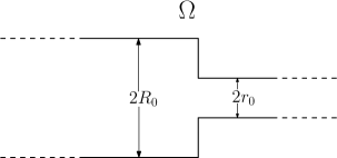
Figure 1: The domain $\Omega$ of Theorem 1.6.

To understand how Equation (AC) relates to hybrid zones, let us sketch its derivation from a biological model. Consider a diploid population (individuals carry chromosomes in pairs) in which a trait subject to natural selection is determined by a single bi-allelic genetic locus. We denote the alleles by $\{a,A\}$, so that there are three possible types in our population: the homozygotes $aa$ and $AA$, and the heterozygotes $aA$. The relative fitnesses of individuals of the different types are given by

$aa$	$aA$	$AA$
$1+\widetilde{s}$	$1$	$1+\theta\widetilde{s}$,

where $\widetilde{s}$ is a small positive constant and $\theta\in(0,1]$. In other words, homozygotes are fitter than heterozygotes, and, if $\theta<1$, individuals carrying $aa$ are fitter than those carrying $AA$. We suppose that the population is at Hardy-Weinberg equilibrium, so that the proportion of individuals of types $aa$, $aA$, and $AA$ are $w^{2}$, $2w(1-w)$, and $(1-w)^{2}$ respectively, where $w$ is the proportion of $a$-alleles in the population. During reproduction, each individual produces a large (effectively infinite) number of germ cells (carrying the same genetic material as the parent), which then split into gametes (carrying just one copy of each chromosome). Each offspring is formed by fusing two gametes picked at random from this pool. In an infinite population, the proportion of $a$-alleles in the offspring population will then be that in the pool of gametes. Assuming that individuals produce a number of gametes proportional to their relative fitness, this is calculated to be

$$\frac{(1+\widetilde{s})w^{2}+w(1-w)}{1+\widetilde{s}w^{2}+\theta\widetilde{s}(1-w)^{2}},$$

and for $\widetilde{s}$ small, we see that the change in frequency of $a$-alleles over a single generation, obtained by subtracting $w$ from this quantity, is

$$\widetilde{s}w(1-w)\big{(}w(1+\theta)-\theta\big{)}+\mathcal{O}(\widetilde{s}^{2}).$$

Equation $(AC)$ is recovered by adding dispersal of offspring, setting $\widetilde{s}(1+\theta)/2=\boldsymbol{s}/N$, $\gamma=(1-\theta)/(1+\theta)$, measuring time in units of $N$ generations, and letting $N$ tend to infinity.

[EFP17] consider the case in which $\theta=1$, and so $\gamma=0$, corresponding to both homozygotes being equally fit. They work on the whole of $\mathbb{R}^{\mathbbm{d}}$. To understand the behaviour of the population over large spatial and temporal scales, they apply a diffusive rescaling. The equation becomes

$$(SAC_{\varepsilon})=\begin{cases}\partial_{t}v^{\varepsilon}=\Delta v^{\varepsilon}+\frac{1}{\varepsilon^{2}}v^{\varepsilon}(1-v^{\varepsilon})(2v^{\varepsilon}-1)&x\in\mathbb{R}^{\mathbbm{d}},\quad t>0,\\ v^{\varepsilon}(x,0)=p(x).\end{cases}$$

To state their result we need some notation. Let $\{\boldsymbol{\Gamma}_{t}:S^{\mathbbm{d}-1}\to\mathbb{R}^{\mathbbm{d}}\}_{0\leq t\leq T}$ be a family of smooth embeddings of the surface of the unit sphere in $\mathbb{R}^{\mathbbm{d}}$ to $\mathbb{R}^{\mathbbm{d}}$, evolving according to mean curvature flow. That is, writing $\mathbf{n}_{t}(s)$ for the unit inward normal vector to $\boldsymbol{\Gamma}_{t}$ at $s$, and $\kappa_{t}(s)$ for the mean curvature of $\boldsymbol{\Gamma}_{t}$ at $s$,

$$\partial_{t}\boldsymbol{\Gamma}_{t}(s)=\kappa_{t}(s)\mathbf{n}_{t}(s).$$

In the biologically relevant case, $\mathbbm{d}=2$, mean curvature flow is just curvature flow. We think of this process as defined up to the fixed time $\mathscr{T}$ at which it first develops a singularity. Let $d(x,t)$ be the signed distance from $x$ to $\boldsymbol{\Gamma}_{t}$, chosen to be negative inside $\boldsymbol{\Gamma}_{t}$ and positive outside. Note that, as sets,

$$\boldsymbol{\Gamma}_{t}=\{x\in\mathbb{R}^{\mathbbm{d}}:d(x,t)=0\}.$$

We require some regularity assumptions on the initial condition $p$ of $(SAC_{\varepsilon})$. Set $\Gamma=\{x\in\mathbb{R}^{\mathbbm{d}}:p(x)=\frac{1}{2}\}$; we shall take $\boldsymbol{\Gamma}_{0}=\Gamma$. We assume that

1. $\Gamma$ is $C^{\alpha}$ for some $\alpha>3$.

2. For $x$ inside $\Gamma$, $p(x)>\tfrac{1}{2}$. For $x$ outside $\Gamma$, $p(x)<\tfrac{1}{2}$.

3. There exist $\eta,\mu>0$ such that, for all $x\in\mathbb{R}^{\mathbbm{d}}$, $|p(x)-\frac{1}{2}|\geq\mu\,\big{(}\text{dist}(x,\Gamma)\wedge\eta\big{)}$.

The following result, proved using probabilistic techniques in [EFP17], is a special case of Theorem 3 of [Che92].

Theorem 1.2.

Let $v^{\varepsilon}$ solve $(SAC_{\varepsilon})$ with initial condition $p$ satisfying the conditions ($\mathscr{C}1$)-($\mathscr{C}3$), and define $\mathscr{T}$, $d(x,t)$ as above. Fix $T^{*}\in(0,\mathscr{T})$ and let $k\in\mathbb{N}$. There exist $\varepsilon_{\mathbbm{d}}(k)>0$, and $a_{\mathbbm{d}}(k),c_{\mathbbm{d}}(k)\in(0,\infty)$ such that for all $\varepsilon\in(0,\varepsilon_{\mathbbm{d}})$ and $t$ satisfying $a_{\mathbbm{d}}\varepsilon^{2}|\log\varepsilon|\leq t\leq T^{*},$

1. for $x$ such that $d(x,t)\leq c_{\mathbbm{d}}\varepsilon|\log\varepsilon|$, we have $v^{\varepsilon}(t,x)\geq 1-\varepsilon^{k}$;

2. for $x$ such that $d(x,t)\geq-c_{\mathbbm{d}}\varepsilon|\log\varepsilon|$, we have $v^{\varepsilon}(t,x)\leq\varepsilon^{k}$.

Remark 1.3.

In fact [Che92] and  [EFP17] choose $p<\tfrac{1}{2}$ within the domain enclosed by $\Gamma$ and $p>\tfrac{1}{2}$ outside. Since Theorem 1.2 concerns the symmetric equation $(SAC_{\varepsilon})$, our statement here is equivalent.

In [Goo18] the approach of [EFP17] is modified to apply to the case when the homozygotes are not equally fit. The proof of Theorem 1.2 compares the solution of $(SAC_{\varepsilon})$ to the solution to the one-dimensional equation started from a Heaviside initial condition, which has a stable limiting form. To understand the results of [Goo18], it is also instructive to consider the one-dimensional version of $(AC)$. Note that the one-dimensional equation

$$\partial_{t}u=\frac{\sigma^{2}}{2}\partial_{xx}u+\boldsymbol{s}u(1-u)\big{(}2u-(1-\gamma)\big{)}$$

has a travelling wave solution of the form:

$$u(x,t)=\frac{1}{2}\left(1-\tanh\left(\sqrt{\frac{\boldsymbol{s}}{2\sigma^{2}}}(x-ct)\right)\right),$$ (2)

where the wavespeed is $c=\gamma\sigma\sqrt{\boldsymbol{s}/2}$. This tells us that if we scale $\sigma$ and/or $\boldsymbol{s}$, then we may also have to scale $\gamma$ in order to obtain a finite wavespeed.

[Goo18] considers the equation

$$\begin{cases}\partial_{t}w^{\varepsilon}=\varepsilon^{1-\ell}\Delta w^{\varepsilon}+\frac{1}{\varepsilon^{1+\ell}}w^{\varepsilon}(1-w^{\varepsilon})(2w^{\varepsilon}-(1-\gamma_{\varepsilon}))&x\in\mathbb{R}^{\mathbbm{d}},\;t>0,\\ w^{\varepsilon}(x,0)=p(x)&x\in\mathbb{R}^{\mathbbm{d}},\end{cases}$$ (3)

where $\gamma_{\varepsilon}=\nu\varepsilon^{\widetilde{\ell}}$ for some non-negative $\nu$ and $\widetilde{\ell}$, with the additional condition that $\nu<1$ when $\widetilde{\ell}=0$, and $\ell=\min(\widetilde{\ell},1)$.

Notice that with these parameters, the one-dimensional wave has speed of $\mathcal{O}(1)$ if $\widetilde{\ell}\leq 1$ and tending to zero as $\varepsilon^{\widetilde{\ell}-1}$ if $\widetilde{\ell}>1$. To state the analogue of Theorem 1.2 in this case, we have to modify our assumptions on $\Gamma$:

1. $\Gamma$ is $C^{\alpha}$ for some $\alpha>3$.

2. For $x$ inside $\Gamma$, $p(x)<\tfrac{1+\gamma_{\varepsilon}}{2}$. For $x$ outside $\Gamma$, $p(x)>\tfrac{1+\gamma_{\varepsilon}}{2}$.

3. There exist $\eta,\mu>0$ such that, for all $x\in\mathbb{R}^{\mathbbm{d}}$, $|p(x)-\frac{1+\gamma_{\varepsilon}}{2}|\geq\mu\,\big{(}\text{dist}(x,\Gamma)\wedge\eta\big{)}$.

We define

$$\nu_{\varepsilon}=\left\{\begin{array}[]{ll}\nu&\mbox{if }\widetilde{\ell}\leq 1,\\ \gamma_{\varepsilon}/\varepsilon&\mbox{if }\widetilde{\ell}\in(1,2],\\ 0&\mbox{if }\widetilde{\ell}>2.\end{array}\right.$$ (4)

Theorem 1.4 ([Goo18], Theorem 2.4).

Let $w^{\varepsilon}$ solve Equation (3) with initial condition $p$ satisfying ($\mathscr{C}1$)’-($\mathscr{C}3$)’, and let

$$\partial_{t}\widetilde{\boldsymbol{\Gamma}}_{t}(s)=(\nu_{\varepsilon}+\kappa_{t}(s))\mathbf{n}_{t}(s),$$ (5)

until the time $\mathscr{T}$ at which $\widetilde{\boldsymbol{\Gamma}}$ develops a singularity. Write $d$ for the signed distance to $\boldsymbol{\Gamma}$ (chosen to be positive outside $\boldsymbol{\Gamma}$). Fix $T^{*}\in(0,\mathscr{T})$. Let $k\in\mathbb{N}$. There exists $\varepsilon_{\mathbbm{d}}(k)>0$, and $a_{\mathbbm{d}}(k),c_{\mathbbm{d}}(k)\in(0,\infty)$ such that for all $\varepsilon\in(0,\varepsilon_{\mathbbm{d}})$ and $t$ satisfying $a_{\mathbbm{d}}\varepsilon^{1+\alpha}|\log\varepsilon|\leq t\leq T^{*},$

1. for $x$ such that $d(x,t)\geq c_{\mathbbm{d}}\varepsilon|\log\varepsilon|$, we have $v^{\varepsilon}(t,x)\geq 1-\varepsilon^{k}$;

2. for $x$ such that $d(x,t)\leq-c_{\mathbbm{d}}\varepsilon|\log\varepsilon|$, we have $v^{\varepsilon}(t,x)\leq\varepsilon^{k}$.

Remark 1.5.

For $\widetilde{\ell}\leq 2$, $\nu_{\varepsilon}$ in (4) and (5) corresponds to the one-dimensional wavespeed derived above. For $\widetilde{\ell}>2$, the wavespeed converges to zero sufficiently quickly as $\varepsilon\to 0$ that we can directly focus on mean curvature flow, and not include the small correction in (5) corresponding to the one-dimensional wavespeed for the result to hold.

When $\widetilde{l}=1$, Theorem 1.4 is a special case of Theorem 1.3 of [AHM64] who consider the generation and propagation of a sharp interface for more general versions of the Allen-Cahn equation with a slightly unbalanced bistable nonlinearity.

Note that $\mathbf{n}_{t}(s)$ is the inward facing normal, so the constant flow along the normal determined by $\nu_{\varepsilon}$ causes contraction of the boundary, and so expansion of the region in which the solution is close to one.

We are now in a position to understand why the expansion of a population might be blocked by an isthmus. As advertised, we shall focus on the case $\widetilde{\ell}=1=\ell$:

$$(AC_{\varepsilon})=\begin{cases}\partial_{t}u^{\varepsilon}=\Delta u^{\varepsilon}+\frac{1}{\varepsilon^{2}}u^{\varepsilon}(1-u^{\varepsilon})(2u^{\varepsilon}-(1-\nu\varepsilon))&x\in\Omega,\;t>0,\\ \partial_{n}u^{\varepsilon}=0&x\in\Omega,\;t>0,\\ u^{\varepsilon}(x,0)={\bf{1}}_{x_{1}\geq 0}&x\in\Omega,\end{cases}$$

with $\Omega$ as in Figure 1. This domain has the advantage of notational simplicity, while allowing us to introduce all the key ideas required to understand conditions for blocking/invasion in much more general domains in the next section.

Our first result shows how the behaviour of $(AC_{\varepsilon})$ on the domain $\Omega$ can be very different from that on the whole of Euclidean space. As $\varepsilon\to 0$, the solution will look increasingly like the indicator function of a region whose boundary evolves according to (5), with the additional condition that it is perpendicular to the boundary $\partial\Omega$ of $\Omega$ where the two intersect. If $r_{0}=R_{0}$ then the solution will simply propagate from right to left. Indeed it will converge to a travelling wave, whose exact form is found by substituting into equation (2). If $R_{0}\gg r_{0}$, then the solution will try to spread out from the opening at $x_{1}=0$. Approximating the solution as above, the interface between the region where $u$ is close to $0$ and where it is close to $1$ is pushed to the left by the constant normal flow, while being pushed back by the mean curvature (a kind of ‘surface tension’). In the limit, these two forces will balance if $\nu=\kappa$, that is precisely when the interface to the left of the origin is a hemispherical shell of radius $r=\frac{\mathbbm{d}-1}{\nu}$. This is, of course, the same as the radius at which the forces will balance for a solution on the whole of $\mathbb{R}^{d}$ started from the indicator function of a sphere. However, working on all of $\mathbb{R}^{d}$ does not give a satisfactory example of blocking, as any perturbation above or below this radius will result in complete invasion or extinction of the dominant phenotype respectively. The blocking that we see in domains such as $\Omega$ is robust to this type of perturbation.

Theorem 1.6.

Let $u^{\varepsilon}$ denote the solution to Equation $(AC_{\varepsilon})$ with $\Omega$ as in Figure 1. Suppose $r_{0}<\frac{\mathbbm{d}-1}{\nu}\wedge R_{0}$. Define

$$N_{\mathbbm{r}}=\{x\in\Omega\,:\,\|x\|=\mathbbm{r},\;x_{1}<0\},$$

where $R_{0}>\mathbbm{r}>r_{0}$, and let $\widehat{d}(x)$ be the signed (Euclidean) distance of any point $x\in\Omega$ to $N_{\mathbbm{r}}$ (chosen to be negative as $x_{1}\to-\infty$). Let $k\in\mathbb{N}$. Then there is $\widehat{\varepsilon}(k)>0$ and $M(k)>0$ such that for all $\varepsilon\in(0,\widehat{\varepsilon})$, and all $t\geq 0$,

$$\mbox{if }x=(x_{1},...,x_{\mathbbm{d}})\in\Omega\mbox{ is such that }d(x)\leq-M(k)\varepsilon|\log(\varepsilon)|\mbox{ then }u^{\varepsilon}(x,t)\leq\varepsilon^{k}.$$

In other words, if the aperture $r_{0}$ is too small, and $R_{0}$ is large enough, then, for sufficiently small $\varepsilon$, blocking occurs. The converse is also true in the following sense.

Theorem 1.7.

Let $u^{\varepsilon}$ denote the solution to Equation $(AC_{\varepsilon})$ with $\Omega$ as in Figure 1. Suppose $r_{0}>\frac{\mathbbm{d}-1}{\nu}$, then for all $x\in\Omega$ and $\delta>0$ there is $\widehat{t}:=\widehat{t}(x_{1},R_{0},r_{0})>0$ and $\widehat{\varepsilon}$ such that, for all $\varepsilon\in(0,\widehat{\varepsilon})$ and $t\geq\widehat{t}$ we have $u^{\varepsilon}(t,x)\geq 1-\delta$.

Together, Theorem 1.6 and Theorem 1.7 say that there is a sharp transition at the critical radius $(\mathbbm{d}-1)/\nu$. A generalisation to a large family of domains can be found in Theorem 1.9 and Theorem 1.10 below.

Remark 1.8.

While, for simplicity and clarity of the proofs, we state Theorem 1.6 as a one-sided inequality, as a by-product of our methods one can obtain a lower bound on the right hand side of the domain. That is, in the context of Theorem 1.6, if $x$ is such that $x_{1}\geq M(k)\varepsilon|\log(\varepsilon)|$, then $u^{\varepsilon}(x,t)\geq 1-\varepsilon^{k}$. The proof follows exactly the same arguments as Theorem 1.7; for more details see Theorem 2.4 in [Goo18]. Biologically, the function $u^{\varepsilon}(x,t)$ models the proportion of a particular type in the population at position $x$ and time $t$. Hence Theorem 1.6 says that, if we have blocking, we have coexistence of the two alleles, with a narrow interface of width $\mathcal{O}(\varepsilon|\log(\varepsilon)|)$ between the $aa$ and $AA$ homozygotes near the opening of the domain. Note this is in sharp contrast to Theorem 1.7, where we have fixation of the type $a$-allele across the whole population.

Other domains

The domain $\Omega$ of Theorem 1.6 is very special. [MNL06] consider a plane curve evolving according to Equation (5) in a two-dimensional cylinder with a periodic saw-toothed boundary. More precisely, they take

$$\Omega_{\delta}=\left\{(x,y)\in\mathbb{R}^{2}:x\in\big{(}-H-h_{\delta}(y),H+h_{\delta}(y)\big{)}\right\},$$

where $H$ is a positive constant and $h_{\delta}(y)=\delta h_{1}(y/\delta)$ with $h_{1}$ being smooth, $1$-periodic, satisfying

$$h_{1}(0)=h_{1}(1)=0,\quad h_{1}(y)\geq 0,\quad\forall y\in\mathbb{R};$$ (6)

see Figure 2 for an illustration. They impose the additional condition that at the points where they meet, the curve and the boundary of the domain are perpendicular, and their convention is that the normal to the curve points into the ‘bottom half’ of the domain. This corresponds to the limit of the solution $u^{\varepsilon}$ of $(AC_{\varepsilon})$ on their domain as $\varepsilon\to 0$.

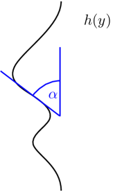
(i)               (ii)

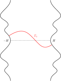
Figure 2: (i) An example of function $h$ for the boundary of the domain (ii) An example of a periodic saw-toothed domain considered by [MNL06]

There will be no travelling wave solution to their equation, in the classical sense, unless the cylinder is flat, and so they define a solution to be a periodic travelling wave if ${\boldsymbol{\Gamma}}_{t+T_{\delta}}(s)={\boldsymbol{\Gamma}}_{t}(s)+\delta$ for some $T_{\delta}>0$. Its effective speed is then $c_{\delta}:=\delta/T_{\delta}$. Recalling that $h_{\delta}(y)=\delta h_{1}(y/\delta)$ and letting $\delta\to 0$, they then investigate the homogenisation limit of the travelling wave, with corresponding speed $c_{0}:=\lim_{\delta\rightarrow 0}c_{\delta}$. They show, in particular, that $c_{0}>0$ if $\nu H>\sin\alpha$ where $\alpha$ is determined by $\tan\alpha=\max_{y}h^{\prime}(y)$, but that the wave is blocked for small enough $\delta$ when $\nu H<\sin\alpha$. In Section 2.8 we shall sketch the proof of the following multidimensional analogue of this blocking result for solutions to $(AC_{\varepsilon})$ in cylindrical domains from our approach.

Theorem 1.9.

Suppose that $u^{\varepsilon}$ solves $(AC_{\varepsilon})$ where $\Omega\subseteq\mathbb{R}^{\mathbbm{d}}$ is defined as in (1) with

$$\phi(x_{1})=\big{\{}\|x^{\prime}\|\leq H+h(-x_{1})\big{\}},$$

and $h$ being a positive, $C^{1}$ (not necessarily periodic) function. Suppose that,

$$\inf_{z>0}\left\{H+h(z)-\left(\frac{\mathbbm{d}-1}{\nu}\right)\frac{h^{\prime}(z)}{\sqrt{1+h^{\prime}(z)^{2}}}\right\}<0.$$ (7)

Fix $k\in\mathbb{N}$. There exist $x_{0}<0$, $\widehat{\varepsilon}(k)>0$ and $M(k)>0$ such that for all $\varepsilon\in(0,\widehat{\varepsilon})$ and $t\geq 0$,

$$\mbox{if }x=(x_{1},...,x_{\mathbbm{d}})\in\Omega\mbox{ is such that }x_{1}\leq x_{0}-M(k)\varepsilon|\log(\varepsilon)|\mbox{ then }u^{\varepsilon}(x,t)\leq\varepsilon^{k}.$$

In other words, the solution is blocked if the cylindrical domain $\Omega$ opens out too quickly. Indeed, in the proof of Theorem 1.9 we compute the angle at which the boundary opens up. We shall see that condition (7) ensures that this angle is ‘big enough’. As a consequence, when (7) holds, we can insert a portion of a spherical shell of radius less than $(\mathbbm{d}-1)/\nu$ into the domain in such a way that expanding the shell radially one stays within the domain, at least for a short time. With this we can adapt the analysis performed for Theorem 1.6 and conclude that there is blocking. Conversely, if the angle is not big enough, we have invasion.

Theorem 1.10.

Suppose that $u^{\varepsilon}$ solves $(AC_{\varepsilon})$ where $\Omega\subseteq\mathbb{R}^{\mathbbm{d}}$ is defined as in (1) with

$$\phi(x_{1})=\big{\{}\|x^{\prime}\|\leq H+h(-x_{1})\big{\}},$$

and $h$ being a positive, $C^{1}$ function. Suppose that

$$\inf_{z>0}\left\{H+h(z)-\left(\frac{\mathbbm{d}-1}{\nu}\right)\frac{h^{\prime}(z)}{\sqrt{1+h^{\prime}(z)^{2}}}\right\}>0$$ (8)

then for all $x\in\Omega$ and $\delta>0$ there is $\widehat{t}:=\widehat{t}(x_{1},R_{0},r_{0})>0$ and $\widehat{\varepsilon}$ such that, for all $\varepsilon\in(0,\widehat{\varepsilon})$ and $t\geq\widehat{t}$ we have $u^{\varepsilon}(t,x)\geq 1-\delta$.

Remark 1.11.

One can check that for $d=2$, if $H\nu<\sin\alpha$, then, for small enough $\delta$, Equation (7) is satisfied and so we see blocking for the domain $\Omega_{\delta}$, whereas if $H\nu>\sin\alpha$ Equation (8) is satisfied for any $\delta>0$ and there is no blocking. Thus we have recovered a multi-dimensional analogue of Theorem 2.1 in [MNL06], with weaker conditions on the function $h$.

While conditions (7) and (8) are hard to verify in general, there are cases where it is trivial to determine if one of them holds. For example, narrowing domains, or those that only narrow beyond the point at which their diameter is first smaller than $2(\mathbbm{d}-1)/\nu$, clearly satisfy (8). See Figure 3 for examples of such domains.

(i)             (ii)

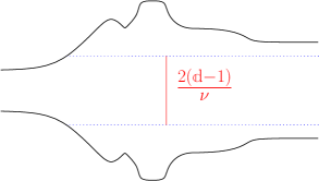
Figure 3: (i) Example of a domain for which the opening only gets narrower. (ii) Example of a domain for which the opening gets smaller once it is less than $(\mathbbm{d}-1)/\nu$.

1.2 Adding noise

In the previous subsection, we justified using equation $(AC_{\varepsilon})$ to model the motion of a hybrid zone in population genetics. However, a deterministic equation like this rests on the assumption of infinite population density. We should like to understand the effects of the random fluctuations caused by reproduction in a finite population.

Several ways of introducing noise into the Allen-Cahn equation have been considered in the literature. [Fun99] considers $(SAC_{\varepsilon})$ on a bounded domain in $\mathbb{R}^{2}$, and with an additional additive noise term of the form $\xi^{\varepsilon}(t)/\varepsilon$, where $\xi^{\varepsilon}$ is centred and smooth in $t$, but behaves like white noise in the limit as $\varepsilon\to 0$. Once again the solution generates an interface as $\varepsilon\to 0$, which Funaki calls randomly perturbed motion by curvature. [Alf+18] consider $(SAC_{\varepsilon})$ with the same form of additive noise as [Fun99], this time on a bounded domain in $\mathbb{R}^{\mathbbm{d}}$. Their results show that, just as in the deterministic case, an interface develops in a very short time, and that the law of motion of the interface is now given by mean curvature flow perturbed by white noise. The profile of the solution near the interface is not destroyed by the random noise, as long as the noise depends only on the time variable. [Lee18] considers a space-time noise, but the noise is smooth in space, and although it is shown that an interface is generated, the law of motion of the interface is not established. [HRW12] consider the equation

$$\partial_{t}u=(\Delta u+u-u^{3})dt+\sigma dW,$$

on $\mathbb{R}^{2}$, where $W$ is a space-time white noise, mollified in space. Setting $v=(1+u)/2$, we recover $(SAC_{\varepsilon})$ with $\varepsilon=1$ and an additional mollified white noise. They show that, if the mollifier is removed, then the solution converges weakly to zero, but that if the intensity of the noise simultaneously converges to zero sufficiently quickly, they recover the solution to the deterministic equation. In other words, unless the noise is small, it can completely destroy the structure of the deterministic equation.

Additive white noise (with or without a spatial component) is not a good model for randomness due to reproduction in a biological population, usually called genetic drift, and so these papers do not resolve the question of whether hybrid zones will still evolve (approximately) according to curvature flow in a population evolving in a two dimensional space. In one spatial dimension, one can justify modelling genetic drift by adding a noise term of the form $\sqrt{u(1-u)}dW$ (for a space-time white noise $W$). In that setting, [Goo18], building on [Fun95], investigates the fluctuations in the position of the hybrid zone (see also [Lee18]). However, the corresponding equation has no solution in two dimensions, and the equation obtained by replacing white noise with a mollified white noise does not arise naturally as a limit of an individual based model. In [EFP17] and [Goo18], a variant of the spatial $\Lambda$-Fleming-Viot process is used to overcome this problem. It is shown that, at least if the genetic drift is sufficiently weak, the (approximate) structure of the deterministic equation is preserved. In Section 3 we use an approach that mimics that used to study the interaction of genic selection with spatial structure in [Eth+17] to provide a stochastic analogue of Theorem 1.6. Furthermore, we prove a complementary result, in which we identify rather precisely the relative strength of genetic drift and selection that results in breakdown in the structure of the deterministic equation.

The key to understanding blocking in the presence of noise is to establish whether a stochastic analogue of Theorem 1.4 holds on the whole of Euclidean space, and so, for the purposes of this introduction, we shall take $\Omega=\mathbb{R}^{\mathbbm{d}}$.

First, we define a version of the Spatial $\Lambda$-Fleming-Viot process with selection that provides a stochastic analogue of the solution to Equation $(AC_{\varepsilon})$. We omit details of the construction, which mirrors the approach taken in [EVY20] in the case of genic selection. At each time $t$, the random function $\{w_{t}(x):\,x\in\mathbb{R}^{\mathbbm{d}}\}$ is defined, up to a Lebesgue null set of $\mathbb{R}^{\mathbbm{d}}$, by

$$w_{t}(x):=\{\text{proportion of type }a\text{ alleles at spatial position }x\text{ at time }t\}.$$

In other words, if we sample an allele from the point $x$ at time $t$, the probability that it is of type $a$ is $w_{t}(x)$.

Remark 1.12.

As is usual for the spatial $\Lambda$-Fleming-Viot processes, $w_{t}(x)$ will only be defined up to a Lebesgue-null set $\mathcal{N}$. Since it is convenient to extend the definition of $w_{t}(x)$ to all of $\mathbb{R}^{\mathbbm{d}}$, we set $w_{t}(x)=0$ for all $x\in\mathcal{N}$.

A construction of an appropriate state space for $x\mapsto w_{t}(x)$ can be found in [VW15]. Using the identification

$$\int_{\mathbb{R}^{\mathbbm{d}}}\big{\{}w_{t}(x)f(x,a)+(1-w_{t}(x))f(x,A)\big{\}}\,dx=\int_{\mathbb{R}^{\mathbbm{d}}\times\{a,A\}}f(x,\kappa)M(dx,d\kappa),$$

this state space is in one-to-one correspondence with the space $\mathcal{M}_{\lambda}$ of measures on $\mathbb{R}^{\mathbbm{d}}\times\{a,A\}$ with ‘spatial marginal’ Lebesgue measure, which we endow with the topology of vague convergence. By a slight abuse of notation, we also denote the state space of the process $(w_{t})_{t\in\mathbb{R}_{+}}$ by ${\cal M}_{\lambda}$.

Definition 1.13 (Spatial $\Lambda$-Fleming-Viot process with selection (SLFVS)).

Fix $u,\gamma\in(0,1]$, $\boldsymbol{s}\in(0,1/(1+\gamma))$, $\mathcal{R}>0$. Let $\mu$ be a finite measure on $(0,\mathcal{R}]$. Let $\Pi$ be a Poisson Point Process on $\mathbb{R}_{+}\times\mathbb{R}^{\mathbbm{d}}\times(0,\mathcal{R}]$ with intensity measure

$$dt\otimes dx\otimes\mu(dr).$$ (9)

The spatial $\Lambda$-Fleming-Viot process with selection (SLFVS) driven by $\Pi$, with selection coefficient $\boldsymbol{s}$ and impact parameter $u$, is the $\mathcal{M}_{\lambda}$-valued process $(w_{t})_{t\geq 0}$ with dynamics given as follows.

If $(t,x,r)\in\Pi$, a reproduction event occurs at time $t$ within the closed ball $B(x,r)$ of radius $r$ centred on $x$. With probability $1-(1+\gamma)\boldsymbol{s}$ the event is neutral, in which case:

1. Choose a parental location $z\in\mathbb{R}^{\mathbbm{d}}$ uniformly at random in $B(x,r)$, and a parental type, $\alpha_{0}$, according to $w_{t-}(z)$. That is $\alpha_{0}=a$ with probability $w_{t-}(z)$ and $\alpha_{0}=A$ with probability $1-w_{t-}(z)$.

2. For every $y\in B(x,r)$, set $w_{t}(y)=(1-u)w_{t-}(y)+u1_{\{\alpha_{0}=a\}}$.

With the complementary probability $(1+\gamma)\boldsymbol{s}$ the event is selective, in which case:

1. Choose three ‘potential’ parental locations $z_{1},z_{2},z_{3}\in\mathbb{R}^{\mathbbm{d}}$ independently and uniformly at random from $B(x,r)$. At each of these sites sample ‘potential’ parental types $\alpha_{1}$, $\alpha_{2}$, $\alpha_{3}$, according to $w_{t-}(z_{1}),w_{t-}(z_{2}),w_{t-}(z_{3})$, respectively. Let $\widehat{\alpha}$ denote the most common allelic type in $\alpha_{1},\alpha_{2},\alpha_{3}$, except that if precisely one of $\alpha_{1}$, $\alpha_{2}$, $\alpha_{3}$, is $a$, with probability $\frac{2\gamma}{3+3\gamma}$ set $\widehat{\alpha}=a$.

2. For every $y\in B(x,r)$ set $w_{t}(y)=(1-u)w_{t-}(y)+u1_{\{\widehat{\alpha}=a\}}$.

Remark 1.14.

Sampling parental locations, and then parental types, is convenient for identifying the dual process of branching and coalescing ancestral lineages that we introduce in Definition 3.1. However, from the perspective of the SLFVS it would be equivalent to sample types independently and uniformly at random from the region affected by the event.

Before going any further, we explain the origin of the reproduction rule in Definition 1.13. Comparing to our justification of Equation $(AC)$, recalling that $w$ is the proportion of $a$-alleles in the population, we first write

$$\boldsymbol{s}w(1-w)(2w-(1-\gamma))\\ =\left((1-(1+\gamma)\boldsymbol{s})w+(1+\gamma)\boldsymbol{s}\left(w^{3}+3w^{2}(1-w)+\left(\frac{2\gamma}{3(1+\gamma)}\right)3w(1-w)^{2}\right)-w\right).$$ (10)

In the SLFVS framework, reproduction events arrive as a Poisson process (as opposed to the deterministic generations times in our justification of $(AC)$). With probability $1-(1+\gamma)\boldsymbol{s}$ an event is neutral, so that the chance that offspring are of type $a$ is simply the probability $w$ that a randomly chosen parent is of type $a$, and we recognise the first term on the right of (10). With probability $(1+\gamma)\boldsymbol{s}$, the event is selective. If we sample three individuals from the population, the probability that the majority are type $a$ is $w^{3}+3w^{2}(1-w)$; whereas the probability that exactly one is type $a$ is $3w(1-w)^{2}$. In the latter case, we multiply further by $2\gamma/(1+\gamma)$ to recover the probability that the offspring are type $a$, and we recognise the second and third terms on the right of (10). In total then, Equation (10) represents the change in proportion of $a$ alleles in the portion of the population replaced during the event.

Remark 1.15.

We could equally have taken two types of selective events, one corresponding to selection against heterozygosity, and one to genic selection. To see why, we rewrite the part of (10) corresponding to selective events as

$$(1+\gamma)\boldsymbol{s}\left(w^{3}+3w^{2}(1-w)+\frac{2\gamma}{3(1+\gamma)}3w(1-w)^{2}-w\right)\\ =\boldsymbol{s}\left(w^{3}+3w^{2}(1-w)-w\right)+\gamma\boldsymbol{s}\left(w^{3}+3w^{2}(1-w)+2w(1-w)^{2}-w\right)\\ =\boldsymbol{s}\left(w^{3}+3w^{2}(1-w)-w\right)+\gamma\boldsymbol{s}\left(w^{2}+2w(1-w)-w\right)$$ (11)

This suggests that with probability $\boldsymbol{s}$ an event corresponds to selection against heterozygosity: three potential parents are sampled and offspring adopt the type of the majority of those individuals; with probability $\gamma\boldsymbol{s}$ an event corresponds to genic selection: two potential parents are sampled and if either of them is type $a$, then the offspring is of type $a$.

Although this leads to the same process of allele frequencies as the apparently more complex mechanism that we introduced in Definition 1.13, in our proof it will be convenient to have a single rule for selective events, based on three potential parents, which will be encoded in the function $g$ of Equation (18) below.

To study the relationship between genetic drift and selection we will introduce two possible scalings for the SLFVS. While the choice of the scaling parameters may seem obscure, once we have introduced a branching and coalescing dual for the SLFVS in Section 3, the reason for these choices will become clear. If in both cases we fix the same values for the parameters that dictate selection (corresponding to $\boldsymbol{s}_{n}$ and $\gamma_{n}$ below), the difference between the two scalings is entirely in the strength of the genetic drift, while the ‘deterministic part’ of the evolution (corresponding to dispersion and selection) is identical. We return to this in Remark 3.7.

Assumption 1.16.

For both regimes, we suppose that $\varepsilon_{n}$ is a sequence such that $\varepsilon_{n}\to 0$ and $(\log n)^{1/2}\varepsilon_{n}\to\infty$ as $n\rightarrow\infty$.

Weak noise/selection ratio

Our first scaling is what we shall call the weak noise/selection ratio regime. In this regime selection overwhelms genetic drift. It mirrors that explored in [EFP17] and is also considered in [Goo18]. For each $n\in\mathbb{N}$, and some $\beta\in(0,1/4)$, we define the finite measure $\mu^{n}$ on $(0,\mathcal{R}_{n}]$, where $\mathcal{R}_{n}=n^{-\beta}\mathcal{R}$, by $\mu^{n}(B)=\mu(n^{\beta}B)$ for all Borel subsets $B$ of $(0,\infty)$. In the weak noise/selection ratio regime the rescaled SLFVS is driven by the Poisson point process $\Pi^{n}$ on $\mathbb{R}^{+}\times\mathbb{R}^{\mathbbm{d}}\times(0,\infty)$ with intensity measure

$$ndt\otimes n^{\beta}dx\otimes\mu^{n}(dr).$$ (12)

Here the linear dimension of the infinitesimal region $dx$ is scaled by $n^{\beta}$ (so that when we integrate, the volume of a region is scaled by $n^{\mathbbm{d}\beta}$). Let $\nu>0$. We denote by $u_{n}$ the impact parameter and by $\boldsymbol{s}_{n}$ the selection parameter at the $n$th stage of the scaling. They will be given by

$$\gamma_{n}=\nu\varepsilon_{n},\qquad u_{n}=\frac{u}{n^{1-2\beta}},\qquad\boldsymbol{s}_{n}=\frac{1}{\varepsilon_{n}^{2}n^{2\beta}}.$$ (13)

Adapting the proof of Theorem 1.11 in [EVY20], and arguments in Section 3 of [EFP17], one can show that under this scaling, for large $n$, the SLFVS will be close to the solution of problem $(AC_{\varepsilon})$.

Strong noise/selection ratio

We shall refer to our second scaling as the strong noise/selection ratio regime. In this regime genetic drift overcomes selection. In this scenario, we consider any sequence of impact parameters $(u_{n})_{n\in\mathbb{N}}\subseteq(0,1)$. Consider $\beta\in(0,1/2)$ and let $\widehat{u}_{n}:=u_{n}n^{1-2\beta}$. We scale time by $n/\widehat{u}_{n}$ and space by $n^{\beta}$. At the $n$th stage of the rescaling, $\Pi^{n}$ is a Poisson measure on $\mathbb{R}^{+}\times\mathbb{R}^{\mathbbm{d}}\times(0,\infty)$ with intensity measure

$$\frac{n}{\widehat{u}_{n}}dt\otimes n^{\beta}dx\otimes\mu^{n}(dr).$$ (14)

We consider a sequence of selection coefficients, $(\boldsymbol{s}_{n})_{n\in\mathbb{N}}\subseteq(0,1)$, satisfying one of the following conditions:

$$\begin{cases}\boldsymbol{s}_{n}n^{2\beta}\rightarrow 0&\liminf_{n\rightarrow\infty}u_{n}\log n<\infty\text{ or }\mathbbm{d}\geq 3,\\ \frac{\boldsymbol{s}_{n}n^{2\beta}}{u_{n}\log n}\rightarrow 0&\liminf u_{n}\log n=\infty\text{ and }\mathbbm{d}=2.\end{cases}$$ (15)

The strength of genetic drift (noise) is determined by the impact parameter. The first case includes some choices of impact that were allowed in the first (weak noise/selection ratio) regime; it is the strength of drift relative to selection that matters. In this regime, we can take the parameters $(\gamma_{n})_{n\in\mathbb{N}}$ that dictate the asymmetry in our selection to be any sequence in $(0,1)$.

The stochastic result

With the two scaling regimes defined we can state a result. Recall that we are working on the whole of Euclidean space.

Theorem 1.17.

Write $\rho_{*}=({\mathbbm{d}}-1)/\nu$. Let $(w_{t}^{n})_{t\geq 0}$ be the scaled SLFVS with initial condition $w_{0}^{n}(x)={\bf{1}}_{B(0,\rho_{*})}(x)$. Fix $t>0$.

1. Under the weak noise/selection ratio regime, for each $k\in\mathbb{N}$, there exist $n_{*}(k)<\infty$, and $d_{*}(k)\in(0,\infty)$, such that for all $n\geq n_{*}$,

   1. for almost every $x$ such that $\|x\|\geq\rho_{*}+d_{*}\varepsilon_{n}|\log\varepsilon_{n}|$, we have $\mathbb{E}\left[w^{n}_{t}(x)\right]\leq\varepsilon_{n}^{k}$;

   2. for almost every $x$ such that $\|x\|\leq\rho_{*}-d_{*}\varepsilon_{n}|\log\varepsilon_{n}|$, we have $\mathbb{E}\left[w^{n}_{t}(x)\right]\geq 1-\varepsilon_{n}^{k}$.

2. Under the strong noise/selection ratio regime, there is $\sigma^{2}>0$ and $n_{*}$, such that for all $n\geq n_{*}$, and all $x\in\mathbb{R}^{\mathbbm{d}}$,

   $$\left|\mathbb{E}_{w_{0}}\left[w_{t}^{n}(x)\right]-\mathbb{P}_{x}[\|W(\sigma^{2}t)\|\leq\rho_{*}]\right|\leq\varepsilon,$$ (16)

   where $(W_{t})_{t\geq 0}$ is a standard Brownian motion in $\mathbb{R}^{\mathbbm{d}}$ and the subscript $x$ on $\mathbb{P}_{x}$ indicates that $W(0)=x$.

More generally, one can show that in the strong noise/selection ratio regime for $x\neq y$, $w_{t}(x)$ and $w_{t}(y)$ decorrelate as $n\to\infty$. In other words, in the weak noise/selection ratio regime the SLFVS behaves approximately as the deterministic equation $(AC_{\varepsilon})$, while in the strong noise/selection ratio regime the genetic drift is strong enough to overcome the effects of selection and it breaks down the interface. (The corresponding breakdown of the interface under the strong noise/selection ratio regime in one dimension requires us to replace $u_{n}\log n$ above by $u_{n}n^{1/2}$.)

Remark 1.18.

As we discuss in a little more detail in Section 3.3, the conditions (15) are essentially optimal. In this regime, if the scaled limits of $\boldsymbol{s}_{n}$ tends to a positive constant, rather than $0$, then we expect the limit to behave like the weak noise/selection regime, except with $\rho^{*}$ replaced by a smaller value.

Everything in this subsection, and in particular Theorem 1.17, has concerned the SLFVS on the whole of $\mathbb{R}^{\mathbbm{d}}$. In the context of the focus of this paper, this result is enough to determine conditions under which genetic drift will break down the effect of the curvature flow and prevent blocking. A technical point that we have to address is that the SLFVS has only previously been studied on all of $\mathbb{R}^{\mathbbm{d}}$ or on a torus. In Appendix C, we present an approach to defining the SLFVS on the domain $\Omega$ of Figure 1 with a natural analogue of the reflecting boundary condition in $(AC_{\varepsilon})$. We call this process the SLFVS on $\Omega$.

Theorem 1.19.

Let $\rho_{*}=({\mathbbm{d}}-1)/\nu$ and suppose $r_{0}<\rho_{*}$. Let $(w_{t}^{n})_{t\geq 0}$ be the scaled SLFVS on $\Omega$ with initial condition $w_{0}^{n}(x)=1_{x_{1}\geq 0}$.

1. Under the weak noise/selection ratio regime, for any $k\in\mathbb{N}$, there exist $n_{*}(k)<\infty$, and $a_{*}(k),d_{*}(k)\in(0,\infty)$ such that for all $n\geq n_{*}$ and all $t>0$ we have that

   $$\text{for almost every }x\text{ such that }x_{1}\leq-d_{*}\varepsilon_{n}|\log\varepsilon_{n}|,\qquad\mathbb{E}\left[w^{n}_{t}(x)\right]\leq\varepsilon_{n}^{k}.$$

2. Under the strong noise/selection ratio regime, a sharp interface does not develop as $n$ goes to infinity. Instead, there is $\sigma^{2}>0$ such that for every $\varepsilon>0$ and $t\geq 0$, there is a reflected Brownian motion, $(W_{t})_{t\geq 0}$, and $n_{*}$, such that for all $n\geq n_{*}$

   $$\left|\mathbb{E}_{w_{0}}\left[w_{t}^{n}(x)\right]-\mathbb{P}_{x}[W(\sigma^{2}t)\geq 0]\right|\leq\varepsilon.$$ (17)

Theorem 1.19 provides an adaptation of Theorem 1.17 to the domain $\Omega$ of Figure 1. In that case, under the weak noise/selection ratio regime, we still see blocking, but in the strong noise/selection ratio regime, the proportion of $a$-alleles spreads approximately according to heat flow in $\Omega$ (with a reflecting boundary condition), and, in particular, blocking no longer occurs.

1.3 Outline of the paper

To prove Theorem 1.6, we proceed as follows. First, in Section 2.1 we provide a stochastic representation for the solution of equation $(AC_{\varepsilon})$. This is entirely analogous to that in [Goo18] for the equation on $\mathbb{R}^{\mathbbm{d}}$. The solution at the point $x$ at time $t$ is the expected result of a ‘voting procedure’ defined on the tree of paths traced out by branching reflecting Brownian motion in $\Omega$ up to time $t$, starting from a single individual at the point $x$. Some immediate properties of the solution that follow from this representation are presented in Section 2.2. In particular, it allows us to compare the solution from different initial conditions, which in turn allows us to bound the solution to $(AC_{\varepsilon})$ from above by that of the same equation with a bigger initial condition. This will be convenient in formalising the idea of the mean curvature flow ‘fighting against’ the constant flow. This is developed in Section 2.3. In Section 2.4 we present a coupling result which is the key to establishing a concrete bound on the effect of the mean curvature flow. With this, we prove the blocking result for the equation with a larger initial condition and so, a fortiori, for $(AC_{\varepsilon})$. We first bound the solution over a small window of time in Section 2.5, and then use a bootstrapping argument in Section 2.6 to show that this bound is uniform in time. Theorem 1.7 is proved in Section 2.7. In Section 2.8 we sketch the extension of these results to more general domains. In particular, we present key elements of the proof of Theorem 1.9.

In Section 3 we turn to the stochastic version of our problem. The results in this section will be on the whole of $\mathbb{R}^{\mathbbm{d}}$. As usual for models of this type, the key to the analysis will be a dual process of branching and coalescing lineages which we introduce in Section 3.1. The duality function relating this process to the SLFVS will involve the same voting procedure that we use for the branching reflecting Brownian motion in the deterministic setting. Theorem 1.17, is proved in Section 3. In the weak noise/selection ratio regime, the key will be to show that asymptotically we no longer see coalescence in the dual process, which is then well-approximated by branching Brownian motion. This tells us that the solution to the stochastic equation will be close to that of $(AC_{\varepsilon})$. In the strong noise/selection ratio regime, branching events in the dual process are quickly annulled by coalescence and, over long time scales, the dual is close to a single Brownian motion. This allows us to approximate the stochastic evolution by heat flow, in sharp contrast to the first regime.

Boundary conditions have not previously been explicitly treated in the SLFVS. As will become clear, the details of what happens at the boundary should not affect our results and so we relegate a description of how one can construct what can be reasonably called an SLFVS with reflecting boundary conditions (for some rather special domains) to the Appendix.

Acknowledgements The third author is supported by the ANID/Doctorado en el extranjero doctoral scholarship, grant number 2018-72190055. The authors are grateful to Sarah Penington for her careful reading of, and helpful comments on, a preliminary version of this work.

2 Deterministic Model

2.1 A stochastic representation of the solution to $(AC_{\varepsilon})$

Our first goal is to present a stochastic representation of the solution of equation $(AC_{\varepsilon})$. This is an essentially trivial adaptation of the representation of the solution to the corresponding equation on $\mathbb{R}^{\mathbbm{d}}$ presented in [Goo18], which builds on [EFP17], which in turn is closely related to results of [DFL86], but we include it here as it will be central to what follows.

The representation is based on ternary branching reflected Brownian motion in $\Omega$. The dynamics of this process has three ingredients:

1. Spatial motion: during its lifetime each particle moves according to a reflected Brownian motion in $\Omega$.

2. Branching rate, $V$: each individual has an exponentially distributed lifetime with parameter $V$.

3. Branching mechanism: when a particle dies it leaves behind (at the location where it died) exactly three offspring. Conditional on the time and place of their birth, the offspring evolve independently of each other, and in the same manner as the parent.

Assumptions 2.1.

1. For consistency with the PDE literature we adopt the convention that all Brownian motions run at speed $2$ (and so have infinitesimal generator $\Delta$).

2. We shall write $\gamma_{\varepsilon}:=\varepsilon\nu$ and set the branching rate $V=(1+\gamma_{\varepsilon})/\varepsilon^{2}$.

The stochastic representation of $(AC_{\varepsilon})$ is reminiscent of the classical representation of the solution to the Fisher-KPP equation in terms of binary branching Brownian motion ([Sko64, McK67]), but now it will depend not just on the leaves of the tree swept out by the branching Brownian motion, but on the whole tree. We need some notation. We write ${\mathbf{W}}(t)$ for the historical process of the ternary branching reflected Brownian motion; that is, ${\mathbf{W}}(t)$ records the spatial position of all individuals alive at time $s$ for all $s\in[0,t]$.

The set of Ulam-Harris labels $\mathcal{U}=\{\emptyset\}\cup\bigcup_{k=1}^{\infty}\{1,2,3\}^{k}$ will be used to label the vertices of the infinite ternary tree, which consists of a single vertex of degree $1$, which we call the root, and every other vertex having degree $4$. The unique path from a given vertex to the root distinguishes exactly one of its four neighbours, and we consider that neighbour to be its parent, and the remaining three neighbours to be its offspring. The root is given label $\emptyset$, and if a vertex has label $(i_{1},...,i_{n})\in\mathcal{U}$, its offspring have labels $(i_{1},...,i_{n},1)$, $(i_{1},...,i_{n},2)$ and $(i_{1},...,i_{n},3)$. For example, $(3,1)$ is the first child of the third child of the initial ancestor $\emptyset$.

Definition 2.2.

We say that $\mathcal{T}$ is a time-labelled ternary tree if $\mathcal{T}$ is a finite subtree of the infinite ternary tree $\mathcal{U}$, and each internal vertex $v$ of the tree is labelled with a time $t_{v}>0$, where $t_{v}$ is strictly greater than the corresponding label of the parent vertex of $v$.

If we ignore the spatial positions of the individuals in our ternary branching reflected Brownian motion, then each realisation of the process traces out a time-labelled ternary tree which records the relatedness (the genealogy) between individuals, and associates a time to each branching event. We use $N(t)\subset{\cal U}$ to denote the set of individuals at time $t$. We abuse notation to write $(W_{i}(t))_{i\in N(t)}$ for the spatial location of the individuals at time $t$ and $(W_{i}(s))_{0\leq s\leq t}$ for the unique path that connects the leaf $i$ to the root. We write $\mathcal{T}({\mathbf{W}}(t))$ for the time-labelled ternary tree determined by the branching structure of ${\mathbf{W}}(t)$.

Now, for a fixed function $p:\mathbb{R}^{\mathbbm{d}}\rightarrow[0,1]$ and parameter $\gamma_{\varepsilon}\in(0,1)$, we define a voting procedure on the tree $\mathcal{T}({\mathbf{W}}(t))$:

1. Each leaf $i$ of $\mathcal{T}({\mathbf{W}}(t))$ independently votes $1$ with probability $p(W_{i}(t))$, and $0$ otherwise.

2. At each branching point in $\mathcal{T}({\mathbf{W}}(t))$ the vote of the parent particle $j$ is the majority vote of the children $(j,1)$,$(j,2)$ and $(j,3)$, unless precisely one of the offspring votes is $1$, in which case the parent votes $1$ with probability $\frac{2\gamma_{\varepsilon}}{3+3\gamma_{\varepsilon}}$, otherwise the parent votes $0$.

This defines an iterative voting procedure, which runs inwards from the leaves of $\mathcal{T}({\mathbf{W}}(t))$ to the root $\emptyset$.

Definition 2.3.

With the voting procedure above, we define $\mathbb{V}_{p}^{\gamma}({\mathbf{W}}(t))$ to be the vote associated to the root $\emptyset$.

Recalling Assumptions 2.1, we use $\mathbb{P}_{x}^{\varepsilon}$ to denote the law of ${\mathbf{W}}$ when started from a single individual at the point $x\in\Omega$. We have the following representation.

Proposition 2.4.

Let $u^{\varepsilon}_{0}:\Omega\rightarrow[0,1]$. Then $u^{\varepsilon}(x,t)=\mathbb{P}^{\varepsilon}_{x}[\mathbb{V}_{u_{0}}^{\gamma}({\mathbf{W}}(t))=1]$ is a solution to the problem $(AC_{\varepsilon})$ with initial condition $u^{\varepsilon}_{0}$.

Proof.

The proof follows a standard pattern (c.f. [Sko64, McK75]), which we now sketch. To ease notation, we write

$$\mathbb{P}_{x}[\mathbb{V}(t)=1]:=\mathbb{P}^{\varepsilon}_{x}[\mathbb{V}_{u^{\varepsilon}_{0}}^{\gamma}({\mathbf{W}}(t))=1].$$

First we check that $u^{\varepsilon}$ satisfies $(AC_{\varepsilon})$ in the interior of $\Omega$. For this, define the function $g$ by

$$g(p_{1},p_{2},p_{3})=p_{1}p_{2}p_{3}+p_{1}p_{2}(1-p_{3})+p_{1}(1-p_{2})p_{3}+(1-p_{2})p_{2}p_{3}\\ +\frac{2\gamma_{\varepsilon}}{3+3\gamma_{\varepsilon}}\Big{[}(1-p_{1})(1-p_{2})p_{3}+(1-p_{1})p_{2}(1-p_{3})+p_{1}(1-p_{2})(1-p_{3})\Big{]}.$$

This is the vote of a branching point given that the three offspring vote $1$ with probabilities $p_{1},p_{2},p_{3}$ respectively. We abuse notation to write $g(p):=g(p,p,p)$. Note that we have the identity:

$$g(p)-p=\frac{1}{1+\gamma_{\varepsilon}}p(1-p)(2p-(1-\gamma_{\varepsilon})),$$ (18)

in which we recognise the non-linearity in $(AC_{\varepsilon})$ divided by $(1+\gamma_{\varepsilon})$ (c.f. the discussion below Definition 1.13).

Fix $t>0$ and $x\in\Omega$. Denoting by $S$ the first branching time of ${\mathbf{W}}$ and partitioning on the events $\{S\leq h\}$, $\{S>h\}$, for small $h$ we obtain

$$\mathbb{P}_{x}[\mathbb{V}(t+h)=1] =\mathbb{P}_{x}\big{[}\mathbb{V}(t+h)=1|S\leq h\big{]}\mathbb{P}[S\leq h]+\mathbb{P}_{x}\big{[}\mathbb{V}(t+h)=1|S>h\big{]}\mathbb{P}[S>h]$$

$$=\mathbb{E}_{x}\big{[}g(\mathbb{P}_{W_{S}}[\mathbb{V}(t)=1])|S\leq h\big{]}(1-e^{-Vh})+\mathbb{E}_{x}\big{[}\mathbb{P}_{W_{h}}[\mathbb{V}(t)=1]\big{]}e^{-Vh},$$

where we have used the notation $V:=\varepsilon^{-2}(1+\gamma_{\varepsilon})$ from Assumptions 2.1. Now, given the regularity of the heat semigroup, and continuity of $g$, if $h$ is small, we have that

$$\mathbb{E}_{x}[g(\mathbb{P}_{W_{S}}[\mathbb{V}(t)=1])|S\leq h]=g(\mathbb{P}_{x}[\mathbb{V}(t)=1])+\mathcal{O}(h).$$

Using this we can compute:

$$\partial_{t}\mathbb{P}_{x}[\mathbb{V}(t)=1] =\lim_{h\to 0}\frac{\mathbb{E}_{x}[\mathbb{P}_{W_{h}}[\mathbb{V}(t)=1]-\mathbb{P}_{x}[\mathbb{V}(t)=1]]}{h}e^{-Vh}$$

$$+\lim_{h\rightarrow 0}\frac{1-e^{-Vh}}{h}\Bigg{\{}g(\mathbb{P}_{x}[\mathbb{V}(t)=1])-\mathbb{P}_{x}[\mathbb{V}(t)=1]\Bigg{\}}$$

$$=\Delta(\mathbb{P}_{\cdot}[\mathbb{V}(t)=1])(x)+V\Big{\{}g(\mathbb{P}_{x}[\mathbb{V}(t)=1])-\mathbb{P}_{x}[\mathbb{V}(t)=1]\Big{\}}$$

and, substituting for $V$ and using identity (18), the equation follows.

The boundary condition is inherited from the reflecting Brownian motion in the Lipschitz domain $\Omega$, see [BH91]. ∎

2.2 Basic results

In this section we record some easy results from [Goo18], adapted to our setting. It will be convenient to be able to refer to these results in the proof of Theorem 1.6.

A one-dimensional travelling wave.

We will later approximate the profile of the solution to $(AC_{\varepsilon})$ in a neighbourhood of the region in which it takes the value $\frac{1-\nu\varepsilon}{2}$ by the one-dimensional function

$$p(x,t)=\Big{(}\exp\left(-\frac{(x+\nu t)}{\varepsilon}\right)+1\Big{)}^{-1}.$$ (19)

Note (c.f. Equation (2)) that this is a travelling wave solution, with speed $-\nu$ and connecting $0$ at $-\infty$ to $1$ at $\infty$, of the one-dimensional equation

$$\partial_{t}u=\Delta u+\frac{1}{\varepsilon^{2}}u(1-u)(2u-(1-\nu\varepsilon)).$$

We will need to control the ‘width’ of the one dimensional wavefront for small $\varepsilon$. This is readily obtained from the explicit form of (19).

Lemma 2.5 ([Goo18], special case of Theorem 2.11).

For all $k\in\mathbb{N}$, and sufficiently small $\varepsilon=\varepsilon(k)>0$,

1. for $z\geq k\varepsilon|\log(\varepsilon)|-\nu t$, we have $p(z,t)\geq 1-\varepsilon^{k}$;

2. for $z\leq-k\varepsilon|\log(\varepsilon)|-\nu t$, we have $p(z,t)\leq\varepsilon^{k}$.

In our case, the proof of this result is a simple calculation. We also need control of the slope of $p(z,t)$.

Proposition 2.6 ([Goo18], special case of Proposition 2.12).

Let $\varepsilon$ be such that

$$\varepsilon<\min\left(\frac{1}{2\nu},\exp\left(-\frac{36}{23}\right)\right).$$

Suppose that, for some $t\in(0,\infty),z\in\mathbb{R}$ we have

$$\left|p(z,t)-\frac{1}{2}\right|\leq\frac{5+\gamma_{\varepsilon}}{12},$$ (20)

and let $w\in\mathbb{R}$ satisfy $|z-w|\leq\varepsilon$. Then

$$\left|p(z,t)-p(w,t)\right|\geq\frac{|z-w|}{48\varepsilon|\log(\varepsilon)|}.$$

Sketch of proof.

Because we have an exact expression for $p$, it is easy to check that the condition (20) is equivalent to

$$|z-\nu t|\leq\varepsilon\log\left(\frac{11+\gamma_{\varepsilon}}{1-\gamma_{\varepsilon}}\right).$$

Also, for $|x-\nu t|\leq A\varepsilon$,

$$|\partial_{x}p(x,t)|\geq\frac{\tfrac{1}{\varepsilon}\exp(A)}{(1+\exp(A))^{2}}.$$

Substituting $A=1+\log((11+\gamma_{\varepsilon})/(1-\gamma_{\varepsilon}))$, we see that for any point $y$ between $z$ and $w$

$$|\partial_{y}p(y,t)|\geq\frac{1}{48\varepsilon}\frac{(11+\gamma_{\varepsilon})(1-\gamma_{\varepsilon})}{9},$$ (21)

where we have used the bound $e<3$. Using the bound on $\varepsilon$ in the statement of the proposition, we can bound the right hand side of (21) below by $1/(48\varepsilon|\log\varepsilon|)$. Now apply the Mean Value Theorem to $p(z,t)-p(w,t)$ to complete the proof. ∎

Denoting by $\mathbf{B}(t)$ the historical process of a one-dimensional ternary branching Brownian motion with branching rate $V=(1+\gamma_{\varepsilon})/\varepsilon^{2}$ and Brownian motions run at rate $2$, the argument in the proof of Proposition 2.4 yields that, for $p(x,t)$ given by (19),

$$\mathbb{P}_{x}^{\varepsilon}[\mathbb{V}^{\gamma}_{p}(\mathbf{B}(t))=1]:=\mathbb{P}_{x}^{\varepsilon}[\mathbb{V}^{\gamma}_{p(\cdot,0)}(\mathbf{B}(t))=1]=p(x,t).$$ (22)

The conclusion of Proposition 2.6 then becomes that for $z$ with

$$\left|\mathbb{P}_{z}^{\varepsilon}\big{[}\mathbb{V}_{p}^{\gamma}(\mathbf{B}(t))=1\big{]}-\frac{1}{2}\right|\leq\frac{5+\gamma_{\varepsilon}}{12},$$

and $w\in\mathbb{R}$ satisfying $|z-w|\leq\varepsilon$,

$$\Big{|}\mathbb{P}_{z}^{\varepsilon}\big{[}\mathbb{V}_{p}^{\gamma}(\mathbf{B}(t))=1\big{]}-\mathbb{P}_{w}^{\varepsilon}\big{[}\mathbb{V}_{p}^{\gamma}(\mathbf{B}(t))=1\big{]}\Big{|}\geq\frac{|z-w|}{48\varepsilon|\log(\varepsilon)|}.$$

In what follows we will always use $\mathbf{B}(t)$ to denote the historical paths of a one dimensional ternary branching Brownian motion, whereas ${\mathbf{W}}(t)$ will denote the historical paths of the multidimensional (reflected) ternary branching Brownian motion.

Results on the voting system

From a probabilistic perspective, the effect of the potential in $(AC_{\varepsilon})$ is captured by the voting mechanism on our tree: the function $g(p)$ amplifies the difference between $p$ and the unstable fixed point $(1-\gamma_{\varepsilon})/2$. As $\varepsilon$ decreases, we see more and more rounds of voting in the tree by time $t$, leading to a rapid transition in the solution $u^{\varepsilon}$ to $(AC_{\varepsilon})$ from values close to $0$ to values close to $1$. We need to control the amplification of $|p-(1-\gamma_{\varepsilon})/2|$ arising from multiple rounds of voting.

We assemble the results that we need related to our voting scheme. It is immediate from equation (18) that if $p<(1-\gamma_{\varepsilon})/2$, then $g(p)<p$, and, iterating, $g^{(n)}(p)$ will be a decreasing sequence in $n$. Our first lemma (whose proof mimics that of Lemma 2.9 in [EFP17]) controls how rapidly it converges to zero as $n$ increases.

Lemma 2.7 ([Goo18], Lemma 2.14).

For all $k\in\mathbb{N}$ there exists $A(k)<\infty$ such that the following hold:

1. for all $\varepsilon\in(0,\tfrac{1-\gamma_{\varepsilon}}{2}]$ and $n\geq A(k)|\log\varepsilon|$ we have

   $$g^{(n)}(\tfrac{1+\gamma_{\varepsilon}}{2}+\varepsilon)\geq 1-\varepsilon^{k}.$$

2. for all $\varepsilon\in(0,\tfrac{1+\gamma_{\varepsilon}}{2}]$ and $n\geq A(k)|\log\varepsilon|$ we have

   $$g^{(n)}(\tfrac{1+\gamma_{\varepsilon}}{2}-\varepsilon)\leq\varepsilon^{k}.$$

For ease of reference, the proof can be found in Appendix A.

It is convenient to record the following easy bound on the function $g$. For $0\leq p_{1},p_{2},p_{3}\leq\frac{1-\gamma_{\varepsilon}}{2}$,

$$g(p_{1},p_{2},p_{3})\leq\max(p_{1},p_{2},p_{3}).$$ (23)

In order to exploit Lemma 2.7, we will need to know how small $\varepsilon$ must be for us to be able to find (with high probability) a regular $n$-generation ternary tree inside $\boldsymbol{W}(t)$. Let ${\cal T}^{reg}_{n}=\bigcup_{k\leq n}\{1,2,3\}^{k}\subseteq\mathcal{U}$ denote the $n$-level regular ternary tree, and for $l\in\mathbb{R}$ set ${\cal T}^{reg}_{l}:={\cal T}^{reg}_{\lceil l\rceil}$. For ${\cal T}$ a time-labelled ternary tree, we write ${\cal T}^{reg}_{l}\subseteq{\cal T}$ to mean that as subtrees of $\mathcal{U}$, ${\cal T}^{reg}_{l}$ is contained inside ${\cal T}$ (ignoring its time labels).

The proof of the following result is a simple modification of that of the corresponding result (Lemma 2.10) in [EFP17].

Lemma 2.8 ([Goo18], Lemma 2.16).

Let $k\in\mathbb{N}$ and $A(k)$ as in Lemma 2.7. Then there exist $a(k)$ and $\widehat{\varepsilon}(k)$ such that for all $\varepsilon\in(0,\widehat{\varepsilon}(k))$ and $t\geq a(k)\varepsilon^{2}|\log(\varepsilon)|$ we have

$$\mathbb{P}^{\varepsilon}\big{[}\mathcal{T}_{A(k)|\log(\varepsilon)|}^{reg}\subseteq\mathcal{T}({\mathbf{W}}(t))\big{]}\geq 1-\varepsilon^{k}.$$

Sketch of proof.

The idea is simple. The time-length of the path to any leaf in the regular tree of height $A(k)|\log\varepsilon|$ is the sum of this number of independent exponentially distributed random variables with parameter $(1+\gamma_{\varepsilon})/\varepsilon^{2}$. Use a large deviation principle for the sum of these exponentials to estimate the probability that a particular leaf in the regular tree has not been born before time $t$ (and therefore is not contained in $\mathcal{T}({\mathbf{W}}(t))$), and then use a union bound to control the probability that there is a leaf of the regular tree not contained in $\mathcal{T}({\mathbf{W}}(t))$. ∎

Monotonicity in the initial condition

The following comparison result will simplify our analysis of the solution of $(AC_{\varepsilon})$.

Proposition 2.9.

Let $u_{0},v_{0}:\Omega\rightarrow[0,1]$ with $u_{0}(x)\leq v_{0}(x)$ for all $x\in\Omega$. Then

$$\mathbb{P}_{x}^{\varepsilon}[\mathbb{V}_{u_{0}}^{\gamma}({\mathbf{W}}(t))=1]\leq\mathbb{P}_{x}^{\varepsilon}[\mathbb{V}_{v_{0}}^{\gamma}({\mathbf{W}}(t))=1]\qquad\forall x\in\Omega.$$

Proof.

An analytic proof would use the maximum principle and monotonicity, but here we present a probabilistic proof based on a simple coupling argument. Since there are so many different sources of randomness in our stochastic representation of solutions, we spell the argument out. Let us write $u(x,t):=\mathbb{P}_{x}^{\varepsilon}[\mathbb{V}_{u_{0}}^{\gamma}(\mathbf{W}(t))=1]$ and $v(x,t):=\mathbb{P}_{x}^{\varepsilon}[\mathbb{V}_{v_{0}}^{\gamma}(\mathbf{W}(t))=1]$. We shall say ‘the probability law defining $u$’ (respectively $v$) to mean the law in which the each of the leaves of ${\mathbf{W}}(t)$ votes $1$ with probability $u_{0}$ (respectively $v_{0}$).

Consider a given realisation of ${\mathbf{W}}(t)$. To determine the vote of a leaf $W_{i}(t)$, we sample $U_{i}$ uniformly on $[0,1]$. If $U_{i}\leq u_{0}(W_{i}(t))$ then the vote of $W_{i}(t)$ is $1$ under the law defining $u$. Similarly, the vote of $W_{i}(t)$ under the law defining $v$ is one if and only if $U_{i}\leq v_{0}(W_{i}(t))$. Notice that since, by assumption, $u_{0}(x)\leq v_{0}(x)$ for all $x\in\Omega$, coupling by using the same uniform random variables $U_{i}$ for determining the leaf votes for $u$ and $v$, all votes that are $1$ under the law defining $u$ are also $1$ under the law defining $v$. Now consider the votes on the interior of the tree. Suppose that the votes of the offspring of a branch are $(i_{1},i_{2},i_{3})$ under $u$ and $(j_{1},j_{2},j_{3})$ under $v$, and $i_{1}+i_{2}+i_{3}\leq j_{1}+j_{2}+j_{3}$. Recall that under our voting procedure, the vote is determined by majority voting unless exactly one vote is one. Evidently, if the majority vote under $u$ is $1$, then it is also $1$ under $v$; and if $j_{1}+j_{2}+j_{3}=0$, then the vote will be zero under both $u$ and $v$. The only case of interest is when $i_{1}+i_{2}+i_{3}=1=j_{1}+j_{2}+j_{3}$. The vote is then determined by a Bernoulli random variable, resulting in a $1$ with probability $2\gamma_{\varepsilon}/(3+3\gamma_{\varepsilon})$. For the final stage of the coupling, we use the same Bernoulli random variable for determining the vote under $u$ and under $v$. This coupling guarantees that if the vote under $u$ is one, then necessarily the vote under $v$ must also be one. Proceeding inductively down the tree ${\mathbf{W}}$, which is a.s. finite, we find that if under $u$ the vote of the root is $1$ then under $v$ it must also be $1$, and the result follows. ∎

2.3 The upper solution

Proposition 2.9 allows us to bound the solution $u$ to $(AC_{\varepsilon})$ on the domain $\Omega$ of Figure 1 by that obtained by starting from a larger initial condition. It is convenient to start from an initial condition that is radially symmetric on the left side of our domain (i.e. when $x_{1}<0$). We set

$$N_{\mathbbm{r}}=\{x\in\Omega\,:\,\|x\|=\mathbbm{r},\;x_{1}<0\},$$

where $R_{0}>\mathbbm{r}>r_{0}$ (see Figure 4). We can then write $\Omega$ as the disjoint union

$$\Omega=\Omega_{+}\sqcup\Omega_{-}\sqcup N_{\mathbbm{r}},$$

where

$$\Omega_{+}=\{x\in\Omega\,:\,\|x\|<\mathbbm{r}\mbox{ or }x_{1}>0\},$$

and

$$\Omega_{-}=\{x\in\Omega\,:\,\|x\|>\mathbbm{r}\mbox{ and }x_{1}<0\}.$$

The signed distance $\widehat{d}$ of any point in $\Omega$ to $N_{\mathbbm{r}}$ is defined up to a change of sign and we impose $\widehat{d}(x)>0$ for all $x$ in $\Omega_{+}$. Here the distance is that inherited from $\mathbb{R}^{\mathbbm{d}}$. Note that for all $x\in\Omega$ such that $x_{1}<0$,

$$\widehat{d}(x)=\mathbbm{r}-\|x\|.$$ (24)

Let the function $\widehat{p}:=\widehat{p}(x)$ satisfy the following conditions:

1. $\widehat{p}(x)=1$ for all $x=(x_{1},...,x_{\mathbbm{d}})\in\Omega$ such that $x_{1}\geq 0$;

2. $\widehat{p}(x)=\frac{1-\gamma_{\varepsilon}}{2}$ for all $x\in N_{\mathbbm{r}}$;

3. $\widehat{p}(x)>\frac{1-\gamma_{\varepsilon}}{2}$ if $\widehat{d}(x)>0$, and $\widehat{p}<\frac{1-\gamma_{\varepsilon}}{2}$ if $\widehat{d}(x)<0$;

4. $\widehat{p}(x)$ is continuous and there exists $\mu,\lambda>0$ such that $|\widehat{p}(x)-\frac{1-\gamma_{\varepsilon}}{2}|\geq\mu\big{(}\text{dist}(x,N_{\mathbbm{r}})\wedge\eta\big{)}$.

The first condition means that $\widehat{p}$ dominates the initial condition for $(AC_{\varepsilon})$; the second and third that $\widehat{p}(1-\widehat{p})\big{(}2\widehat{p}-(1-\gamma_{\varepsilon})\big{)}$ vanishes only on $N_{\mathbbm{r}}$; and the final one is a lower bound on the slope of $\widehat{p}$ in a neighbourhood of $N_{\mathbbm{r}}$. Since $\mathbbm{r}>r_{0}$, one can readily construct a function $\widehat{p}$ that is radially symmetric in $\Omega\cap\{x_{1}<0\}$ and satisfies $(\mathscr{I}1)-(\mathscr{I}4)$. (The first, second and fourth condition are incompatible when $\mathbbm{r}<r_{0}$.)

We are going to show that for $\mathbbm{r}<\frac{\mathbbm{d}-1}{\nu}$, and small enough $\varepsilon$, the solution to

$$(AC^{*}_{\varepsilon})=\begin{cases}\partial_{t}u=\Delta u+\frac{1}{\varepsilon^{2}}u(1-u)(2u-(1-\varepsilon\nu)),\\ u_{0}=\widehat{p}(x),\\ \partial_{n}u=0.\end{cases}$$

is blocked. More precisely:

Theorem 2.10.

Suppose that $r_{0}<\mathbbm{r}<R_{0}\wedge\frac{\mathbbm{d}-1}{\nu}$ and that $\widehat{p}(x)$ satisfies $(\mathscr{I}1)$-$(\mathscr{I}4)$. Fix $k\in\mathbb{N}$. Then there exist $\widehat{\varepsilon}(k)>0$ and $c(k)>0$ such that for all $\varepsilon\in(0,\widehat{\varepsilon})$, $t\in(0,\infty)$,

$$\mbox{for }z\in\Omega\mbox{ such that }d(z)\leq-c(k)\varepsilon|\log(\varepsilon)|,\mbox{ we have }u(z,t)\leq\varepsilon^{k},$$

where $u(z,t)$ solves $(AC^{*}_{\varepsilon})$.

Since $\widehat{p}(x)\geq{\bf{1}}_{x_{1}\geq 0}$, Theorem 1.6 follows from Theorem 2.10 and Proposition 2.9. To prove Theorem 2.10 we will control $u(x,t)$ close to $N_{\mathbbm{r}}$. The key to this will be a coupling argument which will allow us to control the change in the solution over small time intervals in terms of a one-dimensional problem.

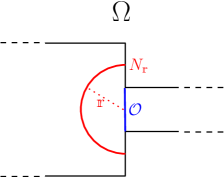
Figure 4: The domain $\Omega$ with $N_{\mathbbm{r}}$ and $\mathcal{O}$ represented in it.

2.4 Coupling around a hemispherical shell

Our next goal is to quantify the effect of the mean curvature flow in ‘pushing back’ the solution of $(AC_{\varepsilon})$. We will need a notation for the ‘opening’ in $\Omega$, which we will denote ${\mathcal{O}}$ (see Figure 4). Recalling that we write $x\in\mathbb{R}^{\mathbbm{d}}$ as $(x_{1},x^{\prime})$ with $x^{\prime}\in\mathbb{R}^{\mathbbm{d}-1}$,

$${\mathcal{O}}=\{x\in\Omega:x_{1}=0,\|x^{\prime}\|<r_{0}\}.$$

The following elementary result will play the role of coupling results in [EFP17] (Proposition 2.14) and [Goo18] (Proposition 2.13), but is completely straightforward since $N_{\mathbbm{r}}$ takes such a simple form.

Lemma 2.11.

Suppose that $r_{0}<\mathbbm{r}<R_{0}$. Let $W$ be a Brownian motion in $\Omega$ and $\beta>0$ such that

$$\beta\leq\frac{\mathbbm{r}-r_{0}}{2}\wedge\frac{R_{0}-\mathbbm{r}}{2}.$$

Define $T_{\beta}$ by

$$T_{\beta}=\inf\{t\geq 0:|\widehat{d}(W_{t})|\geq\beta\}.$$

Then there exists a one-dimensional Brownian motion $\widehat{B}$, started from $\widehat{d}(W_{0})$ such that, for $0\leq s\leq T_{\beta}$,

$$\widehat{B}_{s}-\frac{s(\mathbbm{d}-1)}{\mathbbm{r}+\beta}\geq\widehat{d}(W_{s})\geq\widehat{B}_{s}-\frac{s(\mathbbm{d}-1)}{\mathbbm{r}-\beta}.$$

Proof.

Note that for $s\leq T_{\beta}$, the first coordinate of $W_{s}$, satisfies $(W_{1})_{s}<0$. Indeed, to reach the region in which $(W_{1})_{s}\geq 0$, we must pass through ${\mathcal{O}}$, which requires $|\widehat{d}(W_{s})|\geq\mathbbm{r}-r_{0}>\beta$. In particular, by (24), we have that $\widehat{d}(W_{s})=\mathbbm{r}-\|W_{s}\|$ for all $s\leq T_{\beta}$. Moreover, for $0\leq s<T_{\beta}$, $\|W_{s}\|$ is a (time changed since our Brownian motion runs at rate $2$) Bessel process, whose drift (by definition of $T_{\beta}$) lies in $(\frac{\mathbbm{d}-1}{\mathbbm{r}+\beta},\frac{\mathbbm{d}-1}{\mathbbm{r}-\beta}$), and the result follows. ∎

2.5 Generation of an interface

The next step is to check that the solution to the equation with initial condition $\widehat{p}$ decays rapidly for small times. The proof mimics those that guarantee the formation of an interface in [EFP17] (Proposition 2.16) and [Goo18] (Lemma 2.17). The key is to control the maximal displacement of particles of the ternary branching reflected Brownian motion, with the only twist now being to handle the fact that particles are reflected off the boundary of the domain.

Proposition 2.12.

Let $k\in\mathbb{N}$ and $a(k)$ be given by Lemma 2.8. Then there exists $e(k)$ and $\widehat{\varepsilon}(k)$ such that, for all $\varepsilon\in(0,\widehat{\varepsilon}(k))$, all $s\leq(a(k)+k+1)\varepsilon^{2}|\log(\varepsilon)|$, and all $x\in\Omega$,

$$\mathbb{P}_{x}^{\varepsilon}\Big{[}\exists i\in N(s):\|W_{i}(s)-x\|\geq e(k)\varepsilon|\log(\varepsilon)|\Big{]}\leq\varepsilon^{k}.$$

Proof.

Note that

$$\mathbb{P}_{x}^{\varepsilon}\Big{[}\exists i\in N(s): \|W_{i}(s)-x\|\geq e(k)\varepsilon|\log(\varepsilon)|\Big{]}$$

$$\leq\mathbb{E}^{\varepsilon}\big{[}N(s)\big{]}\mathbb{P}_{x}^{\varepsilon}\Big{[}\|W(s)-x\|\geq e(k)\varepsilon|\log(\varepsilon)|\Big{]}$$

$$=e^{2\frac{s(1+\varepsilon\nu)}{\varepsilon^{2}}}\mathbb{P}_{x}^{\varepsilon}\Big{[}\|W(s)-x\|\geq e(k)\varepsilon|\log(\varepsilon)|\Big{]}$$

$$\leq e^{2(a(k)+k+1)|\log(\varepsilon)|(1+\varepsilon\nu)}\mathbb{P}_{x}^{\varepsilon}\Big{[}\|W(s)-x\|\geq e(k)\varepsilon|\log(\varepsilon)|\Big{]}$$

$$\leq e^{2(a(k)+k+1)|\log(\varepsilon)|(1+\varepsilon\nu)}$$

$$\times\mathbb{P}_{x}^{\varepsilon}\Big{[}\sup_{0\leq s\leq(a(k)+k+1)\varepsilon^{2}|\log(\varepsilon)|}\|W(s)-x\|\geq e(k)\varepsilon|\log(\varepsilon)|\Big{]}.$$ (25)

To bound the last term, consider first $(\widehat{W}_{t})_{t\geq 0}$, defined to be a Brownian motion reflected on the boundary of $\Omega\cap B(x,1)$, which we take to coincide with $(W_{t})_{t\geq 0}$ until the first hitting time of the boundary of $\Omega\cap B(x,1)$. Since $\Omega\cap B(x,1)$ is a bounded domain with Lipschitz boundary, Theorem 2.7 of [BH91] implies the existence of constants $c_{1},c_{2}>0$ (independent of $x$) such that,

$$\mathbb{P}_{x}^{\varepsilon}\Big{[}\sup_{0\leq s\leq(a(k)+k+1)\varepsilon^{2}|\log(\varepsilon)|}\|\widehat{W}(s)-x\| \geq e(k)\varepsilon|\log(\varepsilon)|\Big{]}\leq c_{1}\exp\left(\frac{-e(k)^{2}|\log(\varepsilon)|}{c_{2}(a(k)+k+1)}\right)$$

$$=\varepsilon^{e(k)^{2}(c_{2}(a(k)+k+1))^{-1}}.$$ (26)

Choose $e(k)$ sufficiently large that

$$-2\big{(}a(k)+k+1\big{)}(1+\varepsilon\nu)+\frac{e(k)^{2}}{c_{2}\big{(}a(k)+k+1\big{)}}>k.$$ (27)

Finally, choose $\widehat{\varepsilon}(k)$ sufficiently small that $e(k)\varepsilon|\log(\varepsilon)|<1$ for all $\varepsilon<\widehat{\varepsilon}$. Since $\widehat{W}(s)=W(s)$ until $\widehat{W}(s)$ hits the boundary of $B(x,1)$, this choice of $\widehat{\varepsilon}$ ensures that

$$\left\{\sup_{0\leq s\leq(a(k)+k+1)\varepsilon^{2}|\log(\varepsilon)|}\|\widehat{W}(s)-x\|\geq e(k)\varepsilon|\log(\varepsilon)|\right\}\\ =\left\{\sup_{0\leq s\leq(a(k)+k+1)\varepsilon^{2}|\log(\varepsilon)|}\|W(s)-x\|\geq e(k)\varepsilon|\log(\varepsilon)|\right\}.$$

Substituting (26) in (2.5) and using (27) yields the desired bound. ∎

We are now in a position to prove the rapid decay of the solution to $(AC^{*}_{\varepsilon})$ to the left of $N_{\mathbbm{r}}$.

Proposition 2.13.

Let $k\in\mathbb{N}$. There exist $\widehat{\varepsilon}(k)$, $a(k)$, $b(k)>0$, such that, for all $\varepsilon\in(0,\widehat{\varepsilon}(k))$, setting

$$\delta(k,\varepsilon):=a(k)\varepsilon^{2}|\log(\varepsilon)|\mbox{ and }\delta^{\prime}(k,\varepsilon):=(a(k)+k+1)\varepsilon^{2}|\log(\varepsilon)|,$$

for $t\in[\delta(k,\varepsilon),\delta^{\prime}(k,\varepsilon)]$, and $x$ with $\widehat{d}(x)\leq-b(k)\varepsilon|\log(\varepsilon)|$, $\mathbb{P}_{x}^{\varepsilon}[\mathbb{V}_{\widehat{p}}^{\gamma}({\mathbf{W}}(t))=1]\leq\varepsilon^{k}$.

Proof.

By Lemma 2.8, given $k\in\mathbb{N}$ there exists $a(k)$ and $\widehat{\varepsilon}(k)$ such that, for all $\varepsilon\in(0,\widehat{\varepsilon}(k))$ and $t\geq a(k)\varepsilon^{2}|\log(\varepsilon)|$,

$$\mathbb{P}^{\varepsilon}\big{[}\mathcal{T}_{A(k)|\log(\varepsilon)|}^{reg}\subseteq\mathcal{T}({\mathbf{W}}(t))\big{]}\geq 1-\varepsilon^{k}.$$ (28)

Similarly by Proposition 2.12 there exists $e(k)$ such that, taking a smaller $\widehat{\varepsilon}(k)$ if necessary, for $\varepsilon\in(0,\widehat{\varepsilon}(k))$ and $t\in[\delta(k,\varepsilon),\delta^{\prime}(k,\varepsilon)]$, we have,

$$\mathbb{P}_{x}^{\varepsilon}\Big{[}\exists i\in N(t):\|W_{i}(t)-x\|\geq e(k)\varepsilon|\log(\varepsilon)|\Big{]}\leq\varepsilon^{k}.$$ (29)

Set $b(k)=2e(k)$. Then if $x$ is such that $\widehat{d}(x)\leq-b(k)\varepsilon|\log(\varepsilon)|$ and $\|W_{i}(t)-x\|\leq e(k)\varepsilon|\log(\varepsilon)|$ (noting that this implies that $W_{1}(t)\leq 0$), we obtain (using (24) and the triangle inequality)

$$\widehat{d}(W_{i}(t))=\widehat{d}(x)+\|x\|-\|W_{i}\| \leq\widehat{d}(x)+\|W_{i}(t)-x\|$$

$$\leq-b(k)\varepsilon|\log(\varepsilon)|+e(k)\varepsilon|\log(\varepsilon)|=-e(k)\varepsilon|\log(\varepsilon)|,$$

Reducing $\widehat{\varepsilon}(k)$ if necessary, we can ensure that $\varepsilon<\mu\eta$ with $\mu$, $\eta$ as in $(\mathscr{I}4)$, and $\varepsilon<\mu e(k)\varepsilon|\log(\varepsilon)|$ for $\varepsilon\in(0,\widehat{\varepsilon}(k))$. Then since $\widehat{p}$ satisfies $(\mathscr{I}4)$, we have that

$$\widehat{p}(W_{i}(t))\leq\frac{1-\gamma_{\varepsilon}}{2}-\mu\big{(}|\widehat{d}(W_{i}(t))|\wedge\eta\big{)}\leq\frac{1-\gamma_{\varepsilon}}{2}-\varepsilon.$$

Using (28) and (29), with probability at least $1-2\varepsilon^{k}$, $\mathcal{T}({\mathbf{W}}(t))$ contains a regular tree with at least $A(k)|\log(\varepsilon)|$ generations, and each leaf of $\mathcal{T}({\mathbf{W}}(t))$ votes $1$ with probability at most $\frac{1-\gamma_{\varepsilon}}{2}-\varepsilon$. Recalling from Equation (23), that if $p_{i}\leq\frac{1-\gamma_{\varepsilon}}{2}$ for $i=1,2,3$ then $g_{\gamma_{\varepsilon}}(p_{1},p_{2},p_{3})\leq\max(p_{1},p_{2},p_{3})$, we deduce that in this case, each vertex of $\mathcal{T}$ that corresponds to a leaf of the regular tree of height $A(k)|\log(\varepsilon)|$ votes $1$ with probability at most $\frac{1-\gamma_{\varepsilon}}{2}-\varepsilon$. Lemma 2.7 then gives

$$\mathbb{P}_{x}^{\varepsilon}[\mathbb{V}_{\widehat{p}}^{\gamma}({\mathbf{W}}(t))=1]\leq g_{\gamma_{\varepsilon}}^{(\lceil A(k)|\log(\varepsilon)|\rceil)}\left(\frac{1-\gamma_{\varepsilon}}{2}-\varepsilon\right)+2\varepsilon^{k}\leq 3\varepsilon^{k}.$$

∎

2.6 Blocking (proof of Theorem 2.10)

To prove Theorem 2.10, we establish a comparison between the solution to the multidimensional problem and that of the one-dimensional travelling wavefront (19). This is the content of Proposition 2.14 (corresponding to Proposition 2.17 in [EFP17], and Proposition 2.19 in [Goo18]), whose proof relies on a bootstrapping argument, the key ingredient for which is Lemma 2.15. The radial symmetry simplifies some of the expressions in our setting.

Proposition 2.14.

Let $l\in\mathbb{N}$ with $l\geq 4$ and let $a(l)$ and $\delta(l,\varepsilon)$ be given by Proposition 2.13. There exist $K_{1}(l)$ and $\widehat{\varepsilon}(l,K_{1})>0$ such that, for all $\varepsilon\in(0,\widehat{\varepsilon}(l,K_{1}))$, and $t\in[\delta(l,\varepsilon),\infty)$ we have

$$\sup_{x\in\Omega}\left(\mathbb{P}_{x}^{\varepsilon}[\mathbb{V}_{\widehat{p}}^{\gamma}({\mathbf{W}}(t))=1)]-\mathbb{P}^{\varepsilon}_{\widehat{d}(x)-\nu t+K_{1}\varepsilon|\log(\varepsilon)|}[\mathbb{V}^{\gamma}_{p}(\mathbf{B}(t))=1]\right)\leq\varepsilon^{l},$$

with $\mathbb{V}^{\gamma}_{p}(\mathbf{B}(t))$ as in (22).

The key point here is that after the time $\delta$ that it takes for the interface to develop, we are comparing the multidimensional solution to the stationary one-dimensional interface.

We extend the domain of the function $g$ from $[0,1]$ to $\mathbb{R}$ by setting $g(p)=0$ for $p<0$ and $g(p)=1$ for $p>1$. The following result will be proved after we have proved Proposition 2.14

Lemma 2.15.

Let $l\in\mathbb{N}$ with $l\geq 4$, $K_{1}>0$. There exists $\widehat{\varepsilon}(l,K_{1})>0$ such that for all $\varepsilon\in(0,\widehat{\varepsilon}(l,K_{1}))$, $x\in\Omega$, $s\in[0,(l+1)\varepsilon^{2}|\log(\varepsilon)|]$ and $t\in[s,\infty)$,

$$\mathbb{E}_{x}\left[g\left(\mathbb{P}^{\varepsilon}_{\widehat{d}(W_{s})-\nu(t-s)+K_{1}\varepsilon|\log(\varepsilon)|}[\mathbb{V}_{p}^{\gamma}(\mathbf{B}(t-s)=1]+\varepsilon^{l}\right)\right]\\ \leq\frac{3+5\gamma_{\varepsilon}}{4(1+\gamma_{\varepsilon})}\varepsilon^{l}+\mathbb{E}_{\widehat{d}(x)}^{\varepsilon}\left[g\left(\mathbb{P}^{\varepsilon}_{B_{s}-\nu t+K_{1}\varepsilon|\log(\varepsilon)|}[\mathbb{V}_{p}^{\gamma}(\mathbf{B}(t-s))=1]\right)\right]+1_{s\leq\varepsilon^{3}}\varepsilon^{l}.$$ (30)

Remark 2.16.

In the proof of Proposition 2.14, the time $s$ in Lemma 2.15 will be the time of the first branch in our ternary branching process. In the symmetric case considered in [EFP17], the signed distance between a multi-dimensional Brownian motion at time $s$ and an interface driven by mean curvature flow at time $t-s$ is coupled to a one-dimensional Brownian motion (for small times). Here, $\widehat{d}$ is the signed distance to $N_{\mathbbm{r}}$, which is subject to a mixture of constant flow and curvature flow and so we consider $\widehat{d}(W_{s})-\nu(t-s)$. The inequality (30) will be used to control one round of branching in $\boldsymbol{W}$.

The proof of Proposition 2.14 first compares the multi-dimensional solution to the one-dimensional one over a small time window. It then bootstraps to longer times by conditioning on the first branch time in $\boldsymbol{W}$. The point of Lemma 2.15 is that at the branch time we have $g$ evaluated on the one-dimensional solution plus a small error. If the solution is far from the interface $(1-\gamma_{\varepsilon})/2$, then it is easy to see that the vote will not be changed by the small error. The difficult case is close to the interface, where we make use of estimates of the slope of the (one-dimensional) interface from Proposition 2.6.

Proof of Proposition 2.14.

We follow the proof of Proposition 2.19 of [Goo18] which, in turn, adapts that of Proposition 2.17 of [EFP17].

Take $K_{1}=b(l)+l$, where $b(l)$ is given by Proposition 2.13. Take $\widehat{\varepsilon}$ less than the corresponding $\widehat{\varepsilon}(l)$ in each of Lemma 2.5, Proposition 2.13, and Lemma 2.15.

Define $\delta$ and $\delta^{\prime}$ as in Proposition 2.13. We first show that for $\varepsilon\in(0,\widehat{\varepsilon})$, $t\in[\delta,\delta^{\prime}]$, and $x\in\Omega$ we have

$$\mathbb{P}_{x}^{\varepsilon}[\mathbb{V}^{\gamma}_{\widehat{p}}({\mathbf{W}}(t))=1]\leq\mathbb{P}^{\varepsilon}_{\widehat{d}(x)-\nu t+K_{1}\varepsilon|\log(\varepsilon)|}[\mathbb{V}^{\gamma}_{p}(\mathbf{B}(t))=1]+\varepsilon^{l}.$$ (31)

Indeed, if $\widehat{d}(x)\leq-b(l)\varepsilon|\log(\varepsilon)|$ then, by Proposition 2.13, we have $\mathbb{P}_{x}^{\varepsilon}[\mathbb{V}_{\widehat{p}}({\mathbf{W}}(t))=1]\leq\varepsilon^{l}$. On the other hand if $\widehat{d}(x)\geq-b(l)\varepsilon|\log(\varepsilon)|$ then $\widehat{d}(x)-\nu t+K_{1}\varepsilon|\log(\varepsilon)|\geq-\nu t+l\varepsilon|\log(\varepsilon)|$ (since $K_{1}=b(l)+l$), and so, by Lemma 2.5, the right hand side of (31) is greater than $1$ and hence the inequality obviously holds.

Now consider $t\geq\delta^{\prime}$. Suppose that there exist $t\in[\delta^{\prime},\infty)$ for which the inequality (31) does not hold, that is for which there is $x\in\Omega$ such that

$$\mathbb{P}_{x}^{\varepsilon}[\mathbb{V}^{\gamma}_{\widehat{p}}({\mathbf{W}}(t))=1]-\mathbb{P}^{\varepsilon}_{\widehat{d}(x)-\nu t+K_{1}\varepsilon|\log(\varepsilon)|}[\mathbb{V}^{\gamma}_{p}(\mathbf{B}(t))=1]>\varepsilon^{l}.$$ (32)

Let $T^{\prime}$ be the infimum of such $t$ and choose $T\in[T^{\prime},T^{\prime}+\varepsilon^{l+3}]$ for which (32) holds. By definition there is $x=x(l,\varepsilon)\in\Omega$ such that

$$\mathbb{P}_{x}^{\varepsilon}[\mathbb{V}^{\gamma}_{\widehat{p}}({\mathbf{W}}(T))=1]-\mathbb{P}^{\varepsilon}_{\widehat{d}(x)-\nu T+K_{1}\varepsilon|\log(\varepsilon)|}[\mathbb{V}^{\gamma}_{p}(\mathbf{B}(T))=1]>\varepsilon^{l}.$$

We now seek to show that under this assumption

$$\mathbb{P}_{x}^{\varepsilon}[\mathbb{V}_{\widehat{p}}({\mathbf{W}}(T))=1]\leq\frac{7+9\gamma_{\varepsilon}}{8(1+\gamma_{\varepsilon})}\varepsilon^{l}+\mathbb{P}^{\varepsilon}_{\widehat{d}(x)-\nu T+K_{1}\varepsilon|\log(\varepsilon)|}[\mathbb{V}^{\gamma}_{p}(\mathbf{B}(T))=1].$$ (33)

To establish a contradiction we then choose $\varepsilon$ sufficiently small that $\frac{7+9\gamma_{\varepsilon}}{8(1+\gamma_{\varepsilon})}\varepsilon^{l}<\varepsilon^{l}$, so that (33) contradicts the assumption that (32) is satisified at time $T$.

It remains to prove (33) under the assumption that there exist $t\in[\delta^{\prime},\infty)$ for which (32) holds. We write $S$ for the time of the first branching event in ${\mathbf{W}}(t)$, and $W_{S}$ for the location of the individual that branches at that time. Using the strong Markov property,

$$\mathbb{P}_{x}^{\varepsilon}[\mathbb{V}_{\widehat{p}}^{\gamma}({\mathbf{W}}(T))=1]=\mathbb{E}_{x}^{\varepsilon}\left[g\left(\mathbb{P}_{W_{S}}^{\varepsilon}[\mathbb{V}^{\gamma}_{\widehat{p}}({\mathbf{W}}(T-S))=1]\right){\bf{1}}_{S\leq T-\delta}\right]\\ +\mathbb{E}_{x}^{\varepsilon}[\mathbb{P}_{W_{T-\delta}}^{\varepsilon}[\mathbb{V}^{\gamma}_{\widehat{p}}({\mathbf{W}}(\delta))=1]{\bf{1}}_{S\geq T-\delta}].$$ (34)

As $T-\delta\geq\delta^{\prime}-\delta=(l+1)\varepsilon^{2}|\log(\varepsilon)|$ and $S\sim\mathtt{Exp}((1+\gamma_{\varepsilon})\varepsilon^{-2})$ we can bound the second term in (34) by $\mathbb{P}^{\varepsilon}[S\geq(l+1)\varepsilon^{2}|\log(\varepsilon)|]\leq\varepsilon^{l+1}$. To bound the other term we partition over the event $\{S\leq\varepsilon^{l+3}\}$ (which we note has probability at most $(1+\gamma_{\varepsilon})\varepsilon^{l+1}$) and its complement:

$$\mathbb{E}_{x}^{\varepsilon}\left[g\left(\mathbb{P}_{W_{S}}^{\varepsilon}[\mathbb{V}^{\gamma}_{\widehat{p}}({\mathbf{W}}(T-S))=1]\right){\bf{1}}_{S\leq T-\delta}\right]$$

$$\leq\mathbb{E}_{x}^{\varepsilon}\left[g\left(\mathbb{P}_{W_{S}}^{\varepsilon}[\mathbb{V}_{\widehat{p}}^{\gamma}({\mathbf{W}}(T-S))=1]\right){\bf{1}}_{S\leq T-\delta}{\bf{1}}_{S\geq\varepsilon^{l+3}}\right]+\mathbb{P}^{\varepsilon}[S\leq\varepsilon^{l+3}]$$

$$\leq\mathbb{E}_{x}^{\varepsilon}\left[g\left(\mathbb{P}^{\varepsilon}_{\widehat{d}(W_{S})-\nu(T-s)+K_{1}\varepsilon|\log(\varepsilon)|}[\mathbb{V}^{\gamma}_{p}(\mathbf{B}(T-S))=1]+\varepsilon^{l}\right){\bf{1}}_{S\leq T-\delta}\right]+(1+\gamma_{\varepsilon})\varepsilon^{l+1},$$

where the last line follows from the minimality of $T^{\prime}$ (and noting that if $\varepsilon^{l+3}\leq S\leq T-\delta$, then $T-S\in[\delta,T^{\prime})$), and the monotonicity of $g$.

As the path of a particle is conditionally independent of the time at which it branches, we can condition further on $S$ to obtain

$$\mathbb{E}_{x}^{\varepsilon} \left[g\left(\mathbb{P}^{\varepsilon}_{\widehat{d}(W_{S})-\nu(T-s)+K_{1}\varepsilon|\log(\varepsilon)|}[\mathbb{V}^{\gamma}_{p}(\mathbf{B}(T-S))=1]+\varepsilon^{l}\right){\bf{1}}_{S\leq T-\delta}\right]$$

$$\leq\int_{0}^{(l+1)\varepsilon^{2}|\log(\varepsilon)|}(1+\gamma_{\varepsilon})\varepsilon^{-2}e^{-(1+\gamma_{\varepsilon})\varepsilon^{-2}s}$$

$$\hskip 56.9055pt\times\mathbb{E}_{x}\left[g\left(\mathbb{P}^{\varepsilon}_{\widehat{d}(W_{s})-\nu(T-s)+K_{1}\varepsilon|\log(\varepsilon)|}[\mathbb{V}^{\gamma}_{p}(\mathbf{B}(T-s))=1]+\varepsilon^{l}\right)\right]ds$$

$$\hskip 71.13188pt+\mathbb{P}^{\varepsilon}[S\geq(l+1)\varepsilon^{2}|\log(\varepsilon)|]$$

$$\leq\int_{0}^{(l+1)\varepsilon^{2}|\log(\varepsilon)|}(1+\gamma_{\varepsilon})\varepsilon^{-2}e^{-\varepsilon^{-2}(1+\gamma_{\varepsilon})s}$$

$$\hskip 56.9055pt\times\mathbb{E}_{\widehat{d}(x)}\left[g\left(\mathbb{P}^{\varepsilon}_{B_{s}-\nu T+K_{1}\varepsilon|\log(\varepsilon)|}[\mathbb{V}^{\gamma}_{p}(\mathbf{B}(T-s))=1]+\varepsilon^{l}\right)\right]ds$$

$$\hskip 85.35826pt+\frac{3+5\gamma_{\varepsilon}}{4(1+\gamma_{\varepsilon})}\varepsilon^{l}+\mathbb{P}^{\varepsilon}[S\leq\varepsilon^{3}]\varepsilon^{l}+\varepsilon^{l+1}$$

$$\leq\mathbb{E}_{\widehat{d}(x)}^{\varepsilon}\left[g\left(\mathbb{P}^{\varepsilon}_{B_{S^{\prime}}-\nu T+K_{1}\varepsilon|\log(\varepsilon)|}[\mathbb{V}^{\gamma}_{p}(\mathbf{B}(T-S^{\prime})=1]\right){\bf{1}}_{S^{\prime}\leq T-\delta}\right]$$

$$\hskip 85.35826pt+\frac{3+5\gamma_{\varepsilon}}{4(1+\gamma_{\varepsilon})}\varepsilon^{l}+\varepsilon^{l+1}+\varepsilon^{l+1}(1+\gamma_{\varepsilon}),$$

where the second inequality follows by Lemma 2.15. For the final inequality we have written $S^{\prime}$ for the time of the first branching event in $(\mathbf{B}(s))_{s\geq 0}$ and $B_{S^{\prime}}$ for the position of the ancestor particle at that time. Of course $S^{\prime}$ has the same distribution as $S$, and the inequality follows since $T\geq\delta^{\prime}$ and so $T-\delta\geq(l+1)\varepsilon^{2}|\log(\varepsilon)|$.

Combining these computations, (34) becomes

$$\mathbb{P}_{x}^{\varepsilon} [\mathbb{V}_{p}^{\gamma}({\mathbf{W}}(T))=1]$$

$$\leq\mathbb{E}_{\widehat{d}(x)}^{\varepsilon}\left[g\left(\mathbb{P}^{\varepsilon}_{B_{S^{\prime}}-\nu T+K_{1}\varepsilon|\log(\varepsilon)|}[\mathbb{V}^{\gamma}_{p}(\mathbf{B}(T-S^{\prime})=1]\right){\bf{1}}_{S^{\prime}\leq T-\delta}\right]$$

$$\hskip 142.26378pt+\frac{3+5\gamma_{\varepsilon}}{4(1+\gamma_{\varepsilon})}\varepsilon^{l}+\varepsilon^{l+1}\big{(}2+\gamma_{\varepsilon}\big{)}$$

$$\leq\mathbb{E}^{\varepsilon}_{\widehat{d}(x)-\nu T+K_{1}\varepsilon|\log(\varepsilon)|}[\mathbb{V}^{\gamma}_{p}(\mathbf{B}(T))=1]+\frac{3+5\gamma_{\varepsilon}}{4(1+\gamma_{\varepsilon})}\varepsilon^{l}+\varepsilon^{l+1}\big{(}3+2\gamma_{\varepsilon}\big{)},$$

where, analogously to (34), in the last line we have applied the strong Markov propety at time $S^{\prime}\wedge(T-\delta)$. For sufficiently small $\varepsilon$ we have that $\frac{3+5\gamma_{\varepsilon}}{4(1+\gamma_{\varepsilon})}\varepsilon^{l}+2\varepsilon^{l+1}(1+\varepsilon+\gamma_{\varepsilon}\varepsilon)\leq\frac{7+9\gamma_{\varepsilon}}{8(1+\gamma_{\varepsilon})}\varepsilon^{l}<\varepsilon^{l}$, which completes the proof. ∎

Proof of Lemma 2.15.

Our approach mirrors the proof of Lemma 2.20 of [Goo18], which builds on that of Lemma 2.18 of [EFP17]. The ideas are simple, but they are easily lost in the notation.

Let us write, for $u\geq 0$ and $z\in\mathbb{R}$,

$$\mathbb{Q}_{z}^{\varepsilon,u}=\mathbb{P}_{z}^{\varepsilon}[\mathbb{V}^{\gamma}_{p}(\mathbf{B}(u))=1],$$ (35)

and in what follows we use $\mathbb{Q}_{z}^{u}:=\mathbb{Q}_{z}^{u,\varepsilon}$ when there is no confusion in doing so.

We consider three cases:

1. $\widehat{d}(x)\leq-(l+2\mathbbm{d}(l+1)+K_{1})\varepsilon|\log(\varepsilon)|$.

2. $\widehat{d}(x)\geq(l+2\mathbbm{d}(l+1)+K_{1})\varepsilon|\log(\varepsilon)|$.

3. $|\widehat{d}(x)|\leq(l+2\mathbbm{d}(l+1)+K_{1})\varepsilon|\log(\varepsilon)|$.

Case 1: Let us define

$$A_{x}=\Bigg{\{}\sup_{u\in[0,s]}\|W_{u}-x\|\leq 2\mathbbm{d}(l+1)\varepsilon|\log(\varepsilon)|\Bigg{\}}.$$

We estimate the probability of $A_{x}^{c}$ exactly as in the proof of Proposition 2.12. Indeed reading off from equation (26) with $l=k$, $e(k)=2\mathbbm{d}(k+1)$, $a(k)=0$, we obtain that, for $\widehat{\varepsilon}$ small enough,

$$\mathbb{P}_{x}^{\varepsilon}\big{[}A^{c}_{x}\big{]}\leq c_{1}\varepsilon^{\mathbbm{d}(l+1)}.$$

Now suppose that $A_{x}$ occurs, then the first component of $W_{s}$ is negative, and so, using equation (24),

$$\widehat{d}(W_{s})+K_{1}\varepsilon|\log(\varepsilon)|=\widehat{d}(x)+K_{1}\varepsilon|\log(\varepsilon)|+\widehat{d}(W_{s})-\widehat{d}(x)\\ \leq-(l+2\mathbbm{d}(l+1))\varepsilon|\log(\varepsilon)|+|\widehat{d}(W_{s})-\widehat{d}(x)|\\ =-(l+2\mathbbm{d}(l+1))\varepsilon|\log(\varepsilon)|+\big{|}\|W_{s}\|-\|x\|\big{|}\leq-l\varepsilon|\log(\varepsilon)|.$$ (36)

Therefore, reducing $\widehat{\varepsilon}$ if necessary to ensure that $\gamma_{\widehat{\varepsilon}}\in(0,1)$, applying Lemma 2.5, and using the definition of $g$ and the notation (35),

$$\mathbb{E}_{x}\left[g\left(\mathbb{Q}_{\widehat{d}(W_{s})-\nu(t-s)+K_{1}\varepsilon|\log(\varepsilon)|}^{t-s}+\varepsilon^{l}\right)\right] \leq\mathbb{E}_{x}[g(\varepsilon^{l}+\varepsilon^{l}){\bf{1}}_{A_{x}}]+\mathbb{P}_{x}[A_{x}^{c}]$$

$$\leq 12\varepsilon^{2l}+\frac{4\gamma_{\varepsilon}}{1+\gamma_{\varepsilon}}\varepsilon^{l}+4\mathbbm{d}\varepsilon^{\mathbbm{d}(l+1)}.$$

Reducing $\widehat{\varepsilon}$ still further if necessary, we can certainly arrange that for $\varepsilon\in(0,\widehat{\varepsilon})$ the last line is bounded above by $\frac{3+5\gamma_{\varepsilon}}{4(1+\gamma_{\varepsilon})}\varepsilon^{l}$.

Case $2$: First observe that, using the reflection principle and the standard bound, $\mathbb{P}[Z\geq x]\leq\exp\left(-x^{2}/2\right)$, on the tail of the standard normal distribution,

$$\mathbb{P}_{\widehat{d}(x)}\big{[}B_{s}\leq l\varepsilon|\log(\varepsilon)|\big{]}\leq 2\mathbb{P}_{0}\big{[}B_{(l+1)\varepsilon^{2}|\log\varepsilon|}<-2\mathbbm{d}(l+1)\varepsilon|\log\varepsilon|\big{]}\leq 2\varepsilon^{\mathbbm{d}^{2}(l+1)}.$$

Again applying Lemma 2.5, we obtain

$$\mathbb{E}_{\widehat{d}(x)}\left[g\left(\mathbb{Q}_{B_{s}+K_{1}\varepsilon|\log(\varepsilon)|-\nu t}^{t-s}\right)\right] \geq\mathbb{E}_{\widehat{d}(x)}\left[g\left(\mathbb{Q}_{B_{s}+K_{1}\varepsilon|\log(\varepsilon)|-\nu t}^{t-s}\right){\bf{1}}_{B_{s}\geq l\varepsilon|\log(\varepsilon)|}\right]-2\varepsilon^{\mathbbm{d}^{2}(l+1)}$$

$$\geq g(1-\varepsilon^{l})-2\varepsilon^{\mathbbm{d}^{2}(l+1)}$$

$$=1-\frac{(3+\gamma_{\varepsilon})}{1+\gamma_{\varepsilon}}\varepsilon^{2l}+\frac{2}{1+\gamma_{\varepsilon}}\varepsilon^{3l}-2\varepsilon^{\mathbbm{d}^{2}(l+1)},$$

where the final equality follows from the definition of $g$. Reducing $\widehat{\varepsilon}$ if necessary, we have that for $\varepsilon\in(0,\widehat{\varepsilon})$,

$$\mathbb{E}_{\widehat{d}(x)}\left[g\left(\mathbb{Q}_{B_{s}+K_{1}\varepsilon|\log(\varepsilon)|}^{t-s}\right)\right]\geq 1-\frac{3+5\gamma_{\varepsilon}}{4(1+\gamma_{\varepsilon})}\varepsilon^{l},$$

and in this case the right hand side of (30) is greater than or equal to one, while the left hand side is less than or equal to one by definition.

Case $3$: This is the most difficult case. We combine the coupling of Lemma 2.11 with our lower bound on the slope of the one-dimensional interface.

Again, suppose that $A_{x}$ holds. Since we have chosen $\widehat{\varepsilon}$ small enough that $\mathbbm{r}-r_{0}\geq(l+K_{1}+4\mathbbm{d}(l+1))\varepsilon|\log(\varepsilon)|$ for all $\varepsilon\in(0,\widehat{\varepsilon})$, on the event $A_{x}$ the first component of $W_{s}$ is negative, and, arguing as in (36), using equation (24) we obtain

$$|\widehat{d}(W_{s})|\leq\varepsilon|\log(\varepsilon)|(4\mathbbm{d}(l+1)+l+K_{1}).$$

Choosing $\widehat{\varepsilon}$ still smaller if necessary, for all $\varepsilon\in(0,\widehat{\varepsilon})$,

$$\big{(}4\mathbbm{d}(l+1)+l+K_{1}\big{)}\varepsilon|\log(\varepsilon)|\leq\frac{\mathbbm{r}-r_{0}}{2}\wedge\frac{R_{0}-\mathbbm{r}}{2}.$$ (37)

We write $\beta$ for the quantity on the left hand side of (37) and use Lemma 2.11 to couple the reflected Brownian motion $W$ started at $x\in\Omega$, with a one-dimensional Brownian motion $B$ started at $\widehat{d}(x)$ such that, up to time $T_{\beta}$, we have

$$\widehat{d}(W_{s})\leq B_{s}-\frac{s(\mathbbm{d}-1)}{\mathbbm{r}+\beta}.$$

Combining this with the monotonicity of $g$ and the fact that $\{T_{\beta}\geq s\}\subseteq A_{x}^{c}$ yields

$$\mathbb{E}_{x} \left[g\left(\mathbb{Q}_{\widehat{d}(W_{s})-\nu(t-s)+K_{1}\varepsilon|\log(\varepsilon)|}^{t-s}+\varepsilon^{l}\right)\right]$$

$$\hskip 56.9055pt\leq\mathbb{E}_{\widehat{d}(x)}\left[g\left(\mathbb{Q}_{B_{s}-\nu(t-s)-\frac{s(\mathbbm{d}-1)}{\mathbbm{r}+\beta}+K_{1}\varepsilon|\log(\varepsilon)|}^{t-s}+\varepsilon^{l}\right)\right]+\mathbb{P}_{x}[T_{\beta}\geq s]$$

$$\hskip 56.9055pt\leq\mathbb{E}_{\widehat{d}(x)}\left[g\left(\mathbb{Q}_{B_{s}-\nu(t-s)-\frac{s(\mathbbm{d}-1)}{\mathbbm{r}+\beta}+K_{1}\varepsilon|\log(\varepsilon)|}^{t-s}+\varepsilon^{l}\right)\right]+4\mathbbm{d}\varepsilon^{\mathbbm{d}(l+1)}.$$ (38)

Reducing $\widehat{\varepsilon}$ if necessary, we have that $\mathbbm{r}^{-1}\beta<1$ for all $\varepsilon\in(0,\widehat{\varepsilon})$. Thus

$$(\mathbbm{d}-1)\frac{s}{\mathbbm{r}}\left(\frac{1}{1+\mathbbm{r}^{-1}\beta}\right)\geq\frac{s(\mathbbm{d}-1)}{\mathbbm{r}}(1-\mathbbm{r}^{-1}\beta),$$

and so

$$\nu s-\frac{(\mathbbm{d}-1)s}{\mathbbm{r}+\beta}\leq s\left[\big{(}\nu-\frac{1}{\mathbbm{r}}(\mathbbm{d}-1)\big{)}+\frac{\mathbbm{d}-1}{\mathbbm{r}^{2}}\beta\right].$$ (39)

Recall that, $\mathbbm{r}<(\mathbbm{d}-1)/\nu$ so that $\nu-(\mathbbm{d}-1)/\mathbbm{r}<0$, and so if $\widehat{\varepsilon}$ is small enough, we have that for $\varepsilon\in(0,\widehat{\varepsilon})$

$$\frac{\mathbbm{d}-1}{\mathbbm{r}^{2}}\beta+\varepsilon|\log(\varepsilon)|<\frac{\mathbbm{d}-1}{\mathbbm{r}}-\nu.$$ (40)

In particular, the right hand side of (39) is negative.

Define

$$z=B_{s}-\nu t+s\left[(\nu-\frac{1}{\mathbbm{r}}(\mathbbm{d}-1)+\beta\frac{\mathbbm{d}-1}{\mathbbm{r}^{2}})\right]+K_{1}\varepsilon|(\log(\varepsilon)|.$$

Observe that using (40) we have

$$-s\left[\left(\nu-\frac{1}{\mathbbm{r}}(\mathbbm{d}-1)\right)+\frac{\mathbbm{d}-1}{\mathbbm{r}^{2}}\beta\right] =s\left[\left(\frac{1}{\mathbbm{r}}(\mathbbm{d}-1)-\nu\right)-\frac{\mathbbm{d}-1}{\mathbbm{r}^{2}}\beta\right]$$

$$\geq s\varepsilon|\log(\varepsilon)|,$$

so that

$$z\leq B_{s}-\nu t+(K_{1}-s)\varepsilon|\log\varepsilon|.$$ (41)

Consider the event:

$$E=\left\{\left|\mathbb{Q}_{B_{s}-\nu t+s[(\nu-\frac{1}{\mathbbm{r}}(\mathbbm{d}-1))+\frac{\mathbbm{d}-1}{\mathbbm{r}^{2}}\beta]+K_{1}\varepsilon|\log(\varepsilon)|}^{t-s}-\frac{1}{2}\right|\leq\frac{5+\gamma_{\varepsilon}}{12}\right\}.$$

As explained in [Goo18], although it looks slightly unnatural to take a set centred on the value $1/2$ (about which $g$ is symmetric only in the case when $\gamma=0$), the importance of $E$ is that it spans the interface (where $\mathbb{Q}$ takes the value $(1+\gamma_{\varepsilon})/2$), and on $E^{c}$, $g^{\prime}(\mathbb{Q})<1$.

Suppose first that $E$ occurs. We apply Proposition 2.6 with $z$ as above, and

$$w=z+s\varepsilon|\log(\varepsilon)|\leq B_{s}-\nu t+K_{1}\varepsilon|\log(\varepsilon)|.$$

Note that $|z-w|=s\varepsilon|\log(\varepsilon)|\leq(l+1)\varepsilon^{3}|\log(\varepsilon)|^{2}$, so reducing $\widehat{\varepsilon}$ if necessary so that $(l+1)\varepsilon^{3}|\log(\varepsilon)|^{2}\leq\varepsilon$ for $\varepsilon\in(0,\widehat{\varepsilon})$, Proposition 2.6 implies

$$\mathbb{Q}_{B_{s}-\nu t+K_{1}\varepsilon|\log(\varepsilon)|+s[(\nu-\frac{1}{\mathbbm{r}}(\mathbbm{d}-1))+\frac{\mathbbm{d}-1}{\mathbbm{r}^{2}}\beta]}^{t-s}{\bf{1}}_{E}\leq\left(\mathbb{Q}_{B_{s}-\nu t+K_{1}\varepsilon|\log(\varepsilon)|}^{t-s}-\frac{s}{48}\right){\bf{1}}_{E}.$$ (42)

Now suppose that $E^{c}$ occurs. Since $g^{\prime}(p)=\frac{2}{(1+\gamma_{\varepsilon})}(1-p)(3p+\gamma_{\varepsilon})$, for $p,\delta\geq 0$ with $p+\delta\leq\frac{1-\gamma_{\varepsilon}}{9}$ or $p\geq\frac{8+\gamma_{\varepsilon}}{9}$ it is easy to check that

$$g(p+\delta)\leq g(p)+\frac{2(1+2\gamma_{\varepsilon})}{3(1+\gamma_{\varepsilon})}\delta.$$ (43)

Let $C_{\gamma_{\varepsilon}}=\frac{2(1+2\gamma_{\varepsilon})}{3(1+\gamma_{\varepsilon})}$. Then, reducing $\widehat{\varepsilon}$ if necessary so that $\frac{1-\gamma_{\varepsilon}}{12}+\varepsilon^{l}\leq\frac{1-\gamma_{\varepsilon}}{9}$, for $\varepsilon\in(0,\widehat{\varepsilon})$, we obtain

$$g\left(\mathbb{Q}_{B_{s}-\nu t+K_{1}\varepsilon|\log(\varepsilon)|+s[(\nu-\frac{1}{\mathbbm{r}}(\mathbbm{d}-1))+\frac{\mathbbm{d}-1}{\mathbbm{r}^{2}}\beta]}^{t-s}+\varepsilon^{l}\right){\bf{1}}_{E^{c}}\\ \leq\left(g\Big{(}\mathbb{Q}_{B_{s}-\nu t+K_{1}\varepsilon|\log(\varepsilon)|}^{t-s}\Big{)}+C_{\gamma_{\varepsilon}}\varepsilon^{l}\right){\bf{1}}_{E^{c}},$$ (44)

where we have used (43), (41) and the monotonicity of $g$. Using (38), (42), and (44) we obtain

$$\mathbb{E}_{x} \left[g\left(\mathbb{Q}_{\widehat{d}(W_{s})-\nu(t-s)+K_{1}\varepsilon|\log(\varepsilon)|}^{t-s}+\varepsilon^{l}\right)\right]$$

$$\leq\mathbb{E}_{\widehat{d}(x)}\left[g\left(\mathbb{Q}^{t-s}_{B_{s}-\nu t+K_{1}\varepsilon|\log(\varepsilon)|}-\frac{1}{48}s+\varepsilon^{l}\right){\bf{1}}_{E}\right]$$

$$\hskip 56.9055pt+\mathbb{E}_{\widehat{d}(x)}\left[\left(g\Big{(}\mathbb{Q}^{t-s}_{B_{s}-\nu t+K_{1}\varepsilon|\log(\varepsilon)|}\Big{)}+C_{\gamma_{\varepsilon}}\varepsilon^{l}\right){\bf{1}}_{E^{c}}\right]+4\mathbbm{d}\varepsilon^{\mathbbm{d}(l+1)}$$

$$\leq\mathbb{E}_{\widehat{d}(x)}\left[g\left(\mathbb{Q}^{t-s}_{B_{s}-\nu t+K_{1}\varepsilon|\log(\varepsilon)|}\right)\right]+C_{\gamma_{\varepsilon}}\varepsilon^{l}+\varepsilon^{l}1_{s\leq 48\varepsilon^{l}}+4\mathbbm{d}\varepsilon^{\mathbbm{d}(l+1)},$$

where we have used that $g^{\prime}(p)\leq 1+C_{\gamma_{\varepsilon}}$ for all $p\in[0,1]$. Finally notice that $C_{\gamma_{\varepsilon}}+\frac{1-\gamma_{\varepsilon}}{12(1+\gamma_{\varepsilon})}=\frac{3+5\gamma_{\varepsilon}}{4(1+\gamma_{\varepsilon})}$. Reducing $\widehat{\varepsilon}$ if necessary so that $4\mathbbm{d}\varepsilon^{\mathbbm{d}(l+1)}\leq\frac{1-\gamma_{\varepsilon}}{12(1+\gamma_{\varepsilon})}\varepsilon^{l}$ and $48\varepsilon^{l}\leq\varepsilon^{3}$ for $\varepsilon\in(0,\widehat{\varepsilon})$ (which is possible since $l\geq 4$) completes the proof. ∎

Proof of Theorem 2.10.

Since we are concerned with small $\varepsilon$, it will be sufficient to prove the result for $k\geq 4$.

Let $K_{1}$ be given by Proposition 2.14, and $\widehat{\varepsilon}$ be small enough that Proposition 2.14 and Lemma 2.15 hold. Set $c(k)=k+K_{1}$ so that for any $\varepsilon\in(0,\widehat{\varepsilon})$ and $x\in\Omega$ such that $\widehat{d}(x)\leq-c(k)\varepsilon|\log(\varepsilon)|$ we have that $\widehat{d}(x)+K_{1}\varepsilon|\log(\varepsilon)|\leq-k\varepsilon|\log(\varepsilon)|$. Now choose $a(k)$ as in Proposition 2.14.

For $t\leq a(k)\varepsilon^{2}|\log(\varepsilon)|$ the result holds by Proposition 2.12. Indeed, since by definition $K_{1}=b(k)+k=2e(k)+k$, it holds that $K_{1}\geq e(k)$. From this it follows that, if $\hat{d}(x)\leq c(k)\varepsilon|\log(\varepsilon)|$,

$$\mathbb{P}_{x}^{\varepsilon}\big{[}\mathbb{V}_{\widehat{p}}^{\gamma}({\mathbf{W}}(t))=1)\big{]} \leq\mathbb{P}_{x}^{\varepsilon}\Big{[}\exists i\in N(s):\|W_{i}(s)-x\|\geq e(k)\varepsilon|\log(\varepsilon)|\Big{]}\leq\varepsilon^{k}.$$

On the other hand, for any $t\in[a(k)\varepsilon^{2}|\log(\varepsilon)|,\infty)$,

$$\mathbb{P}_{x}^{\varepsilon}[\mathbb{V}_{\widehat{p}}^{\gamma}({\mathbf{W}}(t))=1)] \leq\varepsilon^{k}+\mathbb{P}_{\widehat{d}(x)-\nu t+K_{1}|\log(\varepsilon)|}^{\varepsilon}[\mathbb{V}_{p}^{\gamma}(\mathbf{B}(t))=1]$$

$$\leq\varepsilon^{k}+\mathbb{P}_{-k\varepsilon|\log(\varepsilon)|-\nu t}^{\varepsilon}[\mathbb{V}_{p}^{\gamma}(\mathbf{B}(t))=1]\leq 2\varepsilon^{k},$$

where the last line is Lemma 2.5. This completes the proof. ∎

2.7 Invasion (proof of Theorem 1.7)

We now turn to the proof of Theorem 1.7. Recall that we are now supposing that the narrower cylinder in the domain $\Omega$ of Figure 1 has radius $r_{0}>(\mathbbm{d}-1)/\nu$. Our proof will mirror the ‘sliding’ technique used in the proof of complete propagation in [BBC16]. The key step is the following proposition, which establishes a lower bound on the solution started from $(1-\varepsilon)$ times the indicator function of a ball, whose radius is greater than $(\mathbbm{d}-1)/\nu$, sitting within $\Omega\cap\{x_{1}>0\}$.

Proposition 2.17.

Suppose that $r_{0}>(\mathbbm{d}-1)/\nu$ and set

$$r^{*}=\frac{r_{0}+(\mathbbm{d}-1)/\nu}{2}.$$

Consider the solution $\widetilde{u}^{\varepsilon}$ to $(AC_{\varepsilon})$ with the initial condition replaced by $\widetilde{u}^{\varepsilon}(x,0)=(1-\varepsilon){\bf{1}}_{B(x^{0},r^{*})}(x),$ where $x^{0}=(x^{0}_{1},\mathbf{0})$ and $\mathbf{0}$ denotes the origin in $\mathbb{R}^{\mathbbm{d}-1}$. Let $\widetilde{\boldsymbol{\Gamma}}$ be the solution to (5) started from the boundary of $B(x^{0},r^{*})$, and $T_{r^{*}}$ be the time at which it is is equal to the boundary of $B(x^{0},\rho^{*})$ with $\rho^{*}$ defined by

$$\rho^{*}=r^{*}+\frac{r_{0}-r^{*}}{4}.$$

There exist constants $a$ and $\widehat{\varepsilon}>0$ such that for all $\varepsilon\in(0,\widehat{\varepsilon})$,

$$\widetilde{u}^{\varepsilon}(x,T_{r^{*}})>1-\varepsilon,\qquad\mbox{for all }x\in B(x^{0},\rho^{*}-a\varepsilon|\log\varepsilon|).$$

Outline of proof.

Choose $\widehat{\varepsilon}$ so that $r_{0}-r^{*}>\widehat{\varepsilon}|\log(\widehat{\varepsilon})|^{2}$.

By reducing $\widehat{\varepsilon}$ if necessary, assume that it is less than $\widehat{\varepsilon}(4)$ in each of Lemma 2.5, and Lemma 2.8; and small enough that the conditions of Proposition 2.6 are satisfied.

Denote the signed distance of the point $y\in\Omega$ to $\widetilde{\boldsymbol{\Gamma}}_{t}$ by $\widetilde{d}_{t}(y)$ (with the convention that $\widetilde{d}_{0}(x^{0})>0$). Set

$$\beta=\frac{r^{*}}{2}\wedge\frac{r_{0}-r^{*}}{2},$$

and

$$\widetilde{T}_{\beta}=\inf\{t\geq 0:\widetilde{d}_{t}(W_{t})\geq\beta\}\wedge T_{r^{*}}.$$

Exactly as in Lemma 2.11, for $0\leq s\leq\widetilde{T}_{\beta}$, there exists a one-dimensional Brownian motion $\widetilde{B}$, started from $\widetilde{d}(W_{0})$ such that

$$\widetilde{B}_{s}-\frac{s(\mathbbm{d}-1)}{\rho^{*}+\beta}\geq\widetilde{d}(W_{s})\geq\widetilde{B}_{s}-\frac{s(\mathbbm{d}-1)}{r^{*}-\beta}.$$ (45)

An argument entirely analogous to the proof of Proposition 2.13 (with $k=4$), where now we bound above the probability that a leaf votes $0$ by $\varepsilon$ (corresponding to it falling within $B(x^{0},r^{*})$) plus the probability that it lies outside $B(x^{0},r^{*})$, yields that by choosing $\widehat{\varepsilon}$ smaller still if necessary, there exist $a,b>0$ such that for all $\varepsilon\in(0,\widehat{\varepsilon})$, setting $\delta=a\varepsilon^{2}|\log(\varepsilon)|$ and $\delta^{\prime}=(a+5)\varepsilon^{2}|\log(\varepsilon)|$, for $t\in[\delta(\varepsilon),\delta^{\prime}(\varepsilon)]$, and $x$ with $\widetilde{d}(x)>b\varepsilon|\log(\varepsilon)|$,

$$\mathbb{P}_{x}^{\varepsilon}[\mathbb{V}_{\widetilde{u}^{\varepsilon}(\cdot,0)}({\mathbf{W}}(t))=1]\geq 1-\varepsilon^{4}.$$

Arguing as in the proof of Lemma 2.15, we can show that there is $K_{1}>0$ such that, choosing $\widehat{\varepsilon}$ still smaller if necessary, for all $\varepsilon\in(0,\widehat{\varepsilon})$, $x\in\Omega$, $s\in[0,5\varepsilon^{2}|\log(\varepsilon)|]$ and $t\in[s,T^{*})$,

$$\mathbb{E}_{x}\left[g\left(\mathbb{P}^{\varepsilon}_{\widetilde{d}(W_{s})-\nu(t-s)-K_{1}\varepsilon|\log(\varepsilon)|}[\mathbb{V}_{p}^{\gamma}(\mathbf{B}(t-s)=0]+\varepsilon^{4}\right)\right]\\ \leq\frac{3+5\gamma_{\varepsilon}}{4(1+\gamma_{\varepsilon})}\varepsilon^{4}+\mathbb{E}_{\widetilde{d}(x)}^{\varepsilon}\left[g\left(\mathbb{P}^{\varepsilon}_{B_{s}-\nu t-K_{1}\varepsilon|\log(\varepsilon)|}[\mathbb{V}_{p}^{\gamma}(\mathbf{B}(t-s))=0]\right)\right]+1_{s\leq\varepsilon^{3}}\varepsilon^{4}.$$ (46)

The argument is once again simpler than the general case considered in [Goo18], since in this setting, over the time interval in which we are interested, $\widetilde{d}$ is simply the distance to the boundary of a ball.

From this we can proceed as in the proof of Proposition 2.14 to show that there exist $K_{1}$ and $\widehat{\varepsilon}>0$ such that, for all $\varepsilon\in(0,\widehat{\varepsilon}$, $t\in[\delta(l,\varepsilon),T_{r^{*}}]$ we have

$$\sup_{x\in\Omega}\left(\mathbb{P}_{x}^{\varepsilon}[\mathbb{V}_{\widetilde{u}^{\varepsilon}(\cdot,0)}^{\gamma}({\mathbf{W}}(t))=0)]-\mathbb{P}^{\varepsilon}_{\widetilde{d}(x)-\nu t-K_{1}\varepsilon|\log(\varepsilon)|}[\mathbb{V}^{\gamma}_{p}(\mathbf{B}(t))=0]\right)\leq\varepsilon^{4},$$

with $\mathbb{V}^{\gamma}_{p}(\mathbf{B}(t))$ as in (22).

Finally, we can complete the proof with an argument that mirrors that of Theorem 2.10. ∎

We are now in a position to prove Theorem 1.7.

Proof of Theorem 1.7.

The idea is simple. We use Proposition 2.17 to provide a series of lower solutions to $(AC_{\varepsilon})$. First take $x^{0}=(r^{*},\mathbf{0})$. By Proposition 2.9, for $\varepsilon<\widehat{\varepsilon}$ the solution to $(AC_{\varepsilon})$ at time $T_{r^{*}}$ dominates $\widetilde{u}^{\varepsilon}(\cdot,T_{r^{*}})$. In particular, it is at least $1-\varepsilon$ on $B(x^{1},r^{*})$, where $x^{1}=(r^{*}-(\rho^{*}-r^{*}-a\varepsilon|\log(\varepsilon)|),\mathbf{0})$. By choosing $\widehat{\varepsilon}$ smaller if necessary, we can certainly arrange that $\|x^{0}-x^{1}\|\geq(r_{0}-r^{*})/8$. Notice also that since $r^{*}>(\mathbbm{d}-1)/\nu$, the time $T_{r^{*}}$ is finite.

We can now simply iterate. The solution to $(AC_{\varepsilon})$ at time $2T_{r^{*}}$ dominates that started from $(1-\varepsilon)$ times the indicator function of the ball of radius $r^{*}$ centred on $x^{1}$, which is at least $(1-\varepsilon)$ on the ball radius $r^{*}$ centred on $x^{2}$, where $\|x^{1}-x^{2}\|\geq(r_{0}-r^{*})/8$ and so on. As illustrated in Figure 5, any point $x\in\Omega$ can be connected to the right half-space by a finite chain of balls in this way, and the result follows. ∎

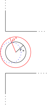
(i)               (ii)

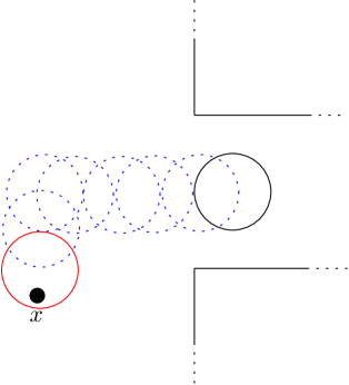
Figure 5: (i) Illustration of Lemma 2.17: started from $(1-\varepsilon)$ times the indicator function of the ball of radius $r^{*}$, at time $T_{r^{*}}$ the solution exceeds $(1-\varepsilon)$ on the larger ball, and a fortiori on the dashed ball of radius $r^{*}$ with centre shifted to the left. (ii) Illustration of how a chain of balls constructed in this way can link any point in $\Omega$ to the $\Omega\cap\{x:x_{1}>0\}$.

2.8 Other domains

The crux of the proof of Theorem 1.6 was the detailed analysis, close to $N_{\mathbbm{r}}$, of the supersolution with initial condition $\widehat{p}$. The key to defining the supersolution was to be able to completely cover the opening $\cal O$ with a hemispherical shell of radius at most $(\mathbbm{d}-1)/\nu$, that is completely contained in $\Omega\cap\{x_{1}<0\}$ (i.e. the portion of $\Omega$ to the left of the origin) and intersects the boundary $\partial\Omega$ at right angles. Evidently, we should be able to prove an entirely analogous result for any domain in which we can identify an appropriate analogue of $N_{\mathbbm{r}}$ and control the solution around it.

The proof would go through completely unchanged for domains of the form $\widehat{\Omega}$ of Figure 6, for example, provided that we could cover the disjoint union of openings by a single hemispherical shell of radius strictly less than $(\mathbbm{d}-1)/\nu$. To see how we can recover an analogue of Theorem 1.6, for more general domains of the form (1), we first consider another special case.

Proposition 2.18.

Let

$$\widetilde{\Omega}=\left\{(x_{1},x^{\prime})\subseteq\mathbb{R}^{\mathbbm{d}}:x^{\prime}\in\phi(x_{1})\subseteq\mathbb{R}^{d}\right\},$$

with

$$\phi(x_{1})=\begin{cases}\|x^{\prime}\|<r_{0}&x_{1}\geq 0\\ \|x^{\prime}\|<r_{0}-x_{1}\tan(\alpha)&x_{1}<0\end{cases},$$

for some $\alpha\in(0,\pi/2]$ and suppose that

$$r_{0}<\frac{\mathbbm{d}-1}{\nu}\sin\alpha.$$ (47)

Let $\mathbbm{r}$ satisfy

$$\frac{r_{0}}{\sin\alpha}<\mathbbm{r}<\frac{\mathbbm{d}-1}{\nu},$$ (48)

and define

$$\widetilde{N}_{\mathbbm{r}}=\Big{\{}x=(x_{1},x^{\prime})\in\widetilde{\Omega}:x_{1}<0,\Big{\|}\left(x_{1}-\frac{r_{0}}{\tan\alpha},x^{\prime}\right)\Big{\|}=\mathbbm{r}\Big{\}}.$$

We write $\widetilde{d}$ for the signed distance to $\widetilde{N}_{\mathbbm{r}}$ (chosen to be negative as $x_{1}\to-\infty$). Let $k\in\mathbb{N}$. Then there is $\widehat{\varepsilon}(k)>0$ and $a(k)$, $M(k)>0$ such that for all $\varepsilon\in(0,\widehat{\varepsilon})$, $t\in(a(k)\varepsilon^{2}|\log(\varepsilon)|,\infty)$ we have that:

$$\text{if}\>\>x=(x_{1},\ldots,x_{\mathbbm{d}})\>\>\text{is such that}\>\>\widetilde{d}(x)\leq-M\varepsilon|\log(\varepsilon)|\>\>\text{then}\>\>w(x,t)\leq\varepsilon^{k}.$$

Remark 2.19.

The condition (47) becomes natural upon observing that any spherical shell intersecting the boundary of $\widetilde{\Omega}$ at right angles must have radius at least $r_{0}/\sin\alpha$,

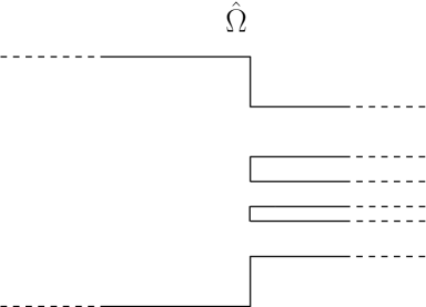
(i)            (ii)

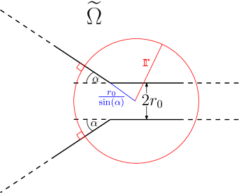
Figure 6: (i)Two dimensional representation of the domain $\widehat{\Omega}$. For $x_{1}>0$, we have multiple cylindrical domains that open into a single cylinder for $x_{1}<0$. (ii) Two dimensional representation of the domain $\widetilde{\Omega}$. It is composed of a cylindrical component on $x_{1}>0$ and a (truncated) cone for $x_{1}<0$.

Sketch of proof.

The proof follows the same pattern as that of Theorem 1.6; first we dominate the solution by one with a larger initial condition, $\widetilde{p}$, then we put an interface with width of order $\varepsilon|\log(\varepsilon)|$ around the set on which the initial condition takes the value $(1-\varepsilon\nu)/2$ and we reproduce the proof of Lemma 2.15 to see how this interface moves.

The initial condition that we take satisfies

1. $\widetilde{p}(x)=1$ for all $x\in\widetilde{\Omega}$ such that $x_{1}\geq 0$;

2. $\widetilde{p}(x)=\frac{1-\gamma_{\varepsilon}}{2}$ for all $x\in\widetilde{N}_{\mathbbm{r}}$.

3. $\widetilde{p}(x)>\frac{1-\gamma_{\varepsilon}}{2}$ if $\widetilde{d}(x)>0$, and $\widetilde{p}<\frac{1-\gamma_{\varepsilon}}{2}$ if $\widetilde{d}(x)<0$.

4. $\widetilde{p}(x)$ is continuous and there exist $\mu,\eta>0$ such that $|\widetilde{p}(x)-\frac{1-\gamma_{\varepsilon}}{2}|\geq\mu(\text{dist}(x,\widetilde{N}_{\mathbbm{r}})\wedge\eta)$.

The conditions of Proposition 2.18 are precisely what is required for these conditions to be compatible.

Our choice of $\widetilde{N}_{\mathbbm{r}}$ enables us to prove the analogue of Theorem 2.10 for $\mathbb{P}_{x}^{\varepsilon}[\mathbb{V}_{\widetilde{p}}^{\gamma}({\mathbf{W}}(t))=1]$ (using the same method). The obvious modification of Lemma 2.11 can then be used to obtain analogues of Lemma 2.15 and 2.14.

∎

Armed with the proof of Proposition 2.18 the main argument behind Theorem 1.9 is easily understood. We recall that the main condition we impose is (7), that is,

$$\inf_{z>0}\left\{H+h(z)-\left(\frac{\mathbbm{d}-1}{\nu}\right)\frac{h^{\prime}(z)}{\sqrt{1+h^{\prime}(z)^{2}}}\right\}<0$$ (49)

(i)             (ii)

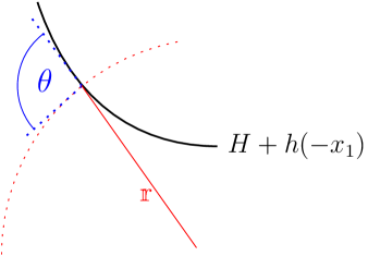
Figure 7: (i) Illustration of the set-up used in Proposition 2.20. The chosen value of $a$ should be obvious from this picture. (ii) Illustration of $\theta$, the angle at which the spherical shell intersects the boundary of $\Omega$

In what follows we recall the notation $\rho^{*}:=(\mathbbm{d}-1)/\nu$. Let

$$N^{*}_{\mathbbm{r},a}=\left\{x=(x_{1},x^{\prime})\in\Omega:x_{1}<0,\|x-(a,0,...,0)\|=\mathbbm{r}\right\},$$

and define $d^{*}_{\mathbbm{r},a}$ to be the distance function to $N^{*}_{\mathbbm{r},a}$ (chosen to be negative as $x_{1}\rightarrow-\infty$).

Proposition 2.20.

Let $W$ be Brownian motion and set

$$T_{\beta}=\inf\left\{t\geq 0:|d^{*}_{\mathbbm{r},a}(W_{t})|\geq\beta\right\}.$$

Then, if (49) holds for some $z>0$, there exist $C,\beta^{*}>0$, $0<\mathbbm{r}<\rho^{*}$, $a<0$ and a Brownian motion $\widehat{B}$, started from $d_{\mathbbm{r},a}^{*}(W_{0})$ such that, for all $0<\beta\leq\beta^{*}$ and $0\leq s\leq T_{\beta}$,

$$d_{\mathbbm{r},a}^{*}(W_{s})\leq\widehat{B}_{s}-\frac{s(\mathbbm{d}-1)}{\mathbbm{r}+\beta}+C\beta s.$$ (50)

Sketch of proof.

Let $z$ be such that

$$H+h(z)-\left(\frac{\mathbbm{d}-1}{\nu}\right)\frac{h^{\prime}(z)}{\sqrt{1+h^{\prime}(z)^{2}}}<0,$$

and set

$$\mathbbm{r}=\frac{1}{2}\left(\frac{(H+h(z))\sqrt{1+h^{\prime}(z)^{2}}}{h^{\prime}(z)}+\rho^{*}\right).$$ (51)

Note that, by our choice of $z$, we have $\mathbbm{r}<\rho^{*}$. Let $a=-z+\sqrt{\mathbbm{r}^{2}-(H+h(z))^{2}}$ and note that $N_{\mathbbm{r},a}^{*}$ intersects the boundary of the domain exactly at the point where the first coordinate is $-z$. See Figure 7(i) for an illustration of this situation.

Choose $\beta^{*}$ small enough that for all $\beta<\beta^{*}$ the distance function $d_{\mathbbm{r},a}^{*}$ satisfies the conditions ($\mathscr{C}1$)-($\mathscr{C}3$) introduced above Theorem 1.2 in $U_{\beta}=\{x:|d_{\mathbbm{r},a}^{*}(x)|\leq\beta\}$. We will now reduce $\beta$ further if necessary to ensure that when $N_{\mathbbm{r},a}^{*}$ intersects the boundary of the domain, the domain is still ‘opening out’ sufficiently fast. More precisely, let $x=(x_{1},x^{\prime})\in\partial\Omega$. Write $v_{1}(x)$ for the vector pointing from $x$ to $(a,0,...0)$, and $v_{2}(x)$ the normal vector to $\partial\Omega$ at $x$. We require that the angle $\theta$ between these two vectors is at least $\pi/2$. See Figure 7(ii) for an illustration. Some cumbersome computations that we defer to Appendix B give that,

$$\langle v_{1}(x),v_{2}(x)\rangle=H+h(-x_{1})+h^{\prime}(-x_{1})(-z-x_{1}-\sqrt{\mathbbm{r}^{2}-(H+h(z))^{2}}).$$ (52)

Note that if $x_{1}=-z$ this gives,

$$H+h(z)-h^{\prime}(z)\sqrt{\mathbbm{r}^{2}-(H+h(z))^{2}}$$

$$<H+h(z)-h^{\prime}(z)\sqrt{\frac{(H+h(z))^{2}\big{(}1+h^{\prime}(z)^{2})}{(h^{\prime}(z))^{2}}-(H+h(z))^{2}}=0,$$

which gives that $\theta$ is bigger than $\pi/2$. In particular, by smoothness of $h$, we can reduce $\beta^{*}$, so that for all $\beta<\beta^{*}$ we have that, for $x=(x_{1},x^{\prime})\in U_{\beta}\cap\partial\Omega$,

$$H+h(-x_{1})+h^{\prime}(-x_{1})(-z-x_{1}-\sqrt{\mathbbm{r}^{2}-(H+h(z))^{2}})\leq 0.$$ (53)

Equation (53) encapsulates that the surface hits the boundary of the domain in such a way that $\theta$ is at least $\pi/2$.

Let $d(x)=\|x-a\|-\mathbbm{r}$ be the distance of $x$ from the circle of radius $\mathbbm{r}$ and centre $a$ in $\mathbb{R}^{\mathbbm{d}}$. We can deduce the following fact: there exists a smooth function $f:\Omega\rightarrow\mathbb{R}$ such that,

$$d^{*}_{\mathbbm{r},a}(x)-d(x)=\beta f(x)\,\,\,\,\,\,\forall x\in U_{\beta}.$$

Indeed, as $d^{*}_{\mathbbm{r},a}$ is a perturbation of at most $\beta$ of $d(x)$ the last equation must hold. In particular, for $x\in U_{\beta}$, there exists a constant $C>0$ such that,

$$\Delta d_{\mathbbm{r},a}^{*}(x)\leq\Delta d(x)+\beta C=\frac{\mathbbm{d}-1}{\|x\|}+\beta C.$$

Then, from Itô’s formula, we obtain that for all $t\leq T_{\beta}$,

$$d_{\mathbbm{r},a}^{*}(W_{t})\leq d_{\mathbbm{r},a}^{*}(W_{0}) +\int_{0}^{t}\nabla d_{\mathbbm{r},a}^{*}(W_{s})\cdot dW_{s}+\int_{0}^{t}\frac{(\mathbbm{d}-1)}{\|W_{s}\|}ds+\beta Ct$$

$$+\int_{0}^{t}\langle\nabla d_{\mathbbm{r},a}^{*}(W_{s}),\hat{n}\rangle dL^{\partial\Omega}_{s}(W_{s}),$$ (54)

where $\hat{n}$ is the inward pointing normal. The first two terms of the right hand side of (54) are the Brownian motion (by Lévy’s characterisation). Since $t<T_{\beta}$, the third term on the right hand side of (54) can be bounded by the drift term on the right hand side of equation (50). To deal with the integral against the local time in (54), we just need to show that $\langle\nabla d_{\mathbbm{r},a}^{*}(W_{s}),\hat{n}\rangle\leq 0$. Indeed, if the line segment from $W_{s}$ to $(a,0...,0)$ intersects $\partial\Omega$, then $\nabla d_{\mathbbm{r},a}^{*}(W_{s})$ is a vector parallel to the surface, in which case the inequality holds trivially. On the other hand, if said line segment does not intersect $\partial\Omega$, then $\nabla d_{\mathbbm{r},a}^{*}(W_{s})$ is a vector going from $W_{s}$ to $(a,0,...,0)$, in which case $\langle\nabla d_{\mathbbm{r},a}^{*}(W_{s}),\hat{n}\rangle\leq 0$, since (53) holds from our choice of $\beta^{*}$. Combining these bounds gives (50) and completes the proof. ∎

From the last result the approach to prove Theorem 1.9 should be obvious. We proceed as in Proposition 2.18 by taking an initial condition similar to $\widetilde{p}$, but now it will be $(1-\gamma_{\varepsilon})/2$ for $x\in N_{\mathbbm{r},a}^{*}$. By Proposition 2.20 we can choose $\mathbbm{r}$ and $a$ such that (50) holds. From this the proof of the result is totally analogous to the one used to prove Proposition 2.18, giving Theorem 1.9.

Invasion under condition (8) can then be handled in a very similar way to the proof of Theorem 1.9.

Sketch of proof Theorem 1.10.

If  (8) holds, then, for all $a$, we can choose $\mathbbm{r}$ as in (51), so that (53) holds with the reverse inequality for points that are close enough to $N_{\mathbbm{r},a}^{*}$. From this and the fact $d_{\mathbbm{r},a}^{*}(x)\geq d(x)$, we can obtain the existence of a Brownian motion $\widehat{B}_{s}$ and a constant $C>0$, such that,

$$d_{\mathbbm{r},a}^{*}(W_{s})\geq\widehat{B}_{s}-\frac{s(\mathbbm{d}-1)}{\mathbbm{r}-\beta}\geq\widehat{B}_{s}-s\nu-sC,$$ (55)

where the last inequality holds for sufficiently small $\beta$ and uses that, in this case, $\mathbbm{r}>\rho^{*}$. Therefore, if we consider $u^{\varepsilon}$i, the solution to $(AC_{\varepsilon})$ with initial condition $u^{\varepsilon}(x,0)=(1-\varepsilon)1_{B(a,\mathbbm{r})}$, we can prove an analogue of Proposition 2.17, using (55) in place of (45). Iterating, we can then deduce an analogue of Theorem 1.7 if (8) holds, thus giving the invasion result. ∎

3 Stochastics

We now turn to the SLFVS. As we have seen in the deterministic setting, the crucial step in determining whether or not there will be blocking is to understand the interplay between the selection against heterozygosity and the selective advantage of $aa$-homozygotes over $AA$-homzogotes in a small neighbourhood of a critical radius in which the influence of the boundary of the domain is unimportant. In this section we therefore focus on the SLFVS on the whole of Euclidean space, relegating a discussion of other domains (and, in particular, a suitable definition of the SLFVS on domains with boundary) to Appendix C.

3.1 The dual process

At the core of the proof of Theorem 1.15 was the duality between the deterministic equation $(AC_{\varepsilon})$ and ternary branching (reflected) Brownian motion endowed with a voting mechanism. In an entirely analogous way, we wish to exploit the duality between the SLFVS and a system of branching and coalescing lineages endowed with a similar voting mechanism.

The process of branching and coalescing lineages is driven by (the time-reversal of) the Poisson Point Process of events that determined the dynamics in the SLFVS. Recall that $\Pi^{n}$ is a Poisson point process on $\mathbb{R}_{+}\times\mathbb{R}^{\mathbbm{d}}\times(0,\mathcal{R}_{n})$, whose intensity is given by (12) in the weak noise/selection ratio regime, and by (14) in the strong noise/selection ratio regime. To emphasize that the dual process runs ‘backwards in time’, we shall write $\overleftarrow{\Pi}^{n}$ for the time-reversal of $\Pi^{n}$, which of course has the same intensity as $\Pi^{n}$. The impact, asymmetry and selection parameters $(u_{n})_{n\in\mathbb{N}}$, $(\gamma_{n})_{n\in\mathbb{N}}$, $(\boldsymbol{s}_{n})_{n\in\mathbb{N}}$ are given in (13) in the weak noise/selection ratio regime, or fulfil the condition (15) in the strong noise/selection ratio regime.

Definition 3.1.

(SLFVS dual) For $n\in\mathbb{N}$, the process $(\mathcal{P}_{t}^{n})_{t\geq 0}$ is the $\bigcup_{l\geq 1}(\mathbb{R}^{\mathbbm{d}})^{l}$-valued Markov process with dynamics defined as follows.

The process starts from a single individual at the point $x\in\mathbb{R}^{\mathbbm{d}}$. We write $\mathcal{P}^{n}_{t}=(\xi^{n}_{1}(t),\ldots,\xi^{n}_{N(t)}(t))$, where the random number $N(t)\in\mathbb{N}$ is the number of individuals alive at time $t$, and $\{\xi^{n}_{i}(t)\}_{i=1}^{N(t)}$ are their locations. For each $(t,x,r)\in\overleftarrow{\Pi}^{n}$, the corresponding event is neutral with probability $1-(1+\gamma_{n})\boldsymbol{s}_{n}$, in which case:

1. for each $\xi_{i}^{n}(t-)\in B(x,r)$, independently mark the corresponding individual with probability $u_{n}$;

2. if at least one individual is marked, all marked individuals coalesce into a single offspring, whose location is chosen uniformly in $B(x,r)$.

With the complementary probability $(1+\gamma_{n})\boldsymbol{s}_{n}$, the event is selective, in which case:

1. for each $\xi^{n}_{i}(t-)\in B(x,r)$, independently mark the corresponding individual with probability $u_{n}$;

2. if at least one individual is marked, all of the marked individuals are replaced by a total of three offspring, whose locations are drawn independently and uniformly in $B(x,r)$.

In both cases, if no individual is marked, then nothing happens.

Remark 3.2.

From the perspective of the SLFVS, it would be more natural to call the individuals created during a reproduction event in the dual process ‘parents’ (or ‘potential parents’), as they are situated at the locations from which the parental alleles are sampled. We choose to call them offspring in order to emphasize that the dual process plays the same role as ternary branching Brownian motion in the deterministic setting, and, indeed, much of the proof of Theorem 2.10 carries over with minimal changes to the SLFVS setting.

Just as for the deterministic setting, the duality relation that we exploit is between the SLFVS and the historical process of branching and coalescing lineages,

$$\Xi^{n}(t):=(\mathcal{P}^{n}_{s})_{0\leq s\leq t}.$$

We write $\mathbb{P}_{x}$ for the law of $\Xi^{n}$ when $\mathcal{P}^{n}_{0}$ is the single point $x$, and $\mathbb{E}_{x}$ for the corresponding expectation.

Just as for the branching process, we can use Ulam-Harris labels to define lines of descent from the root individual at $x$ through $\mathcal{P}^{n}$. More precisely, for $\boldsymbol{i}=(i_{1},i_{2},\ldots)\in\{1,2,3\}^{\mathbb{N}}$, we write $(\xi^{n}_{\boldsymbol{i}}(\cdot))_{0\leq s\leq t}\subseteq\Xi^{n}(t)$ for the $\mathbb{R}^{\mathbbm{d}}$-valued path which jumps to the location of the (unique) offspring when the individual in $\mathcal{P}^{n}_{s}$ at its location is affected by a neutral event, and to the location of the $i_{k}$th offspring, the $k$th time that it is affected by a selective event. From the perspective of the SLFVS, $\xi_{\boldsymbol{i}}^{n}$ is an ancestral lineage, and we shall use the terminology lineage below.

Let $p:\mathbb{R}^{\mathbbm{d}}\to[0,1]$. The voting procedure on $\Xi^{n}(t)$ is a natural modification of the one that we defined for the ternary branching Brownian motion:

1. Each leaf of $\Xi^{n}(t)$ independently votes $1$ with probability $p(\xi_{i}(t))$, and $0$ otherwise;

2. at each neutral event in $\overleftarrow{\Pi}^{n}$, all marked individuals adopt the vote of the offspring;

3. at each selective event in $\overleftarrow{\Pi}^{n}$, all marked individuals adopt the majority vote of the three offspring, unless precisely one vote is $1$, in which case they all vote $1$ with probability $\frac{2\gamma_{n}}{3+3\gamma_{n}}$, otherwise they vote $0$.

This defines an iterative voting procedure, which runs inwards from the ‘leaves’ of $\Xi^{n}(t)$ to the ancestral individual $\emptyset$ situated at the point $x$.

Definition 3.3.

With the voting procedure described above, we define $\mathbb{V}_{p}(\Xi^{n}(t))$ to be the vote associated to the root $\emptyset$.

We should like to have an analogue of the stochastic representation of the solution to $(AC_{\varepsilon})$ of Proposition 2.4 for the SLFVS, but recall from Remark 1.12 that the SLFVS is only defined up to a Lebesgue null set, and so we cannot expect such a representation at every point of $\mathbb{R}^{\mathbbm{d}}$. However, a weak version of the representation is valid. The following result is easily proved using the approach introduced to prove Proposition 1.7 in [EVY20] (the corresponding result in the case of genic selection).

Theorem 3.4.

The SLFVS driven by $\Pi^{n}$, $(w^{n}_{t}(x),x\in\mathbb{R}^{\mathbbm{d}})_{t\geq 0}$, is dual to the process $(\Xi^{n}(t))_{t\geq 0}$ of Definition 3.1 in the sense that for every $\psi\in C(\mathbb{R}^{\mathbbm{d}})\cap L^{1}(\mathbb{R}^{\mathbbm{d}})$, we have

$$\mathbb{E}_{p}\left[\int_{\Omega}\psi(x)w^{n}_{t}(x)\,dx\right]=\int_{\Omega}\psi(x)\mathbb{E}_{x}\left[\mathbb{V}_{p}\left(\Xi^{n}(t)\right)\right]\,dx=\int_{\Omega}\psi(x)\mathbb{P}_{x}\left[\mathbb{V}_{p}\big{(}\Xi^{n}(t)\big{)}=1\right]\,dx.$$ (56)

Remark 3.5.

Note that the expectations on the left and right of Equation (56) are taken with respect to different measures. The subscripts on the expectations are the initial values for the processes on each side.

The duality reduces the proof of Theorem 1.17 to the following analogue of Theorem 2.10.

Theorem 3.6.

Define $\rho_{*}=({\mathbbm{d}}-1)/\nu$ and let $\widehat{p}(x)=1_{B(0,\rho_{*})}(x)$.

1. Under the weak noise/selection ratio regime, for any $k\in\mathbb{N}$, there exist $n_{*}(k)<\infty$, and $d_{*}(k)\in(0,\infty)$, such that for all $n\geq n_{*}$ and all $t>0$,

   $$\text{for all }x\in\mathbb{R}^{\mathbbm{d}}\text{ with }\|x\|\geq\rho_{*}+d_{*}\varepsilon_{n}|\log\varepsilon_{n}|,\text{ we have }\mathbb{P}_{x}\left[\mathbb{V}_{\widehat{p}}(\Xi^{n}(t))=1\right]\leq\varepsilon_{n}^{k}.$$

   $$\text{for all }x\in\mathbb{R}^{\mathbbm{d}}\text{ with }\|x\|\leq\rho_{*}-d_{*}\varepsilon_{n}|\log\varepsilon_{n}|,\text{ we have }\mathbb{P}_{x}\left[\mathbb{V}_{\widehat{p}}(\Xi^{n}(t))=1\right]\geq 1-\varepsilon_{n}^{k}.$$

2. Under the strong noise/selection ratio regime, there is a constant $\sigma^{2}>0$ such that for every fixed $t>0$ and $\varepsilon>0$ there is a Brownian motion, $(W_{s})_{s\geq 0}$, and $n_{*}\in\mathbb{N}$, such that for all $n\geq n_{*}$

   $$\Big{|}\mathbb{P}_{x}\big{[}\mathbb{V}_{\widehat{p}}(\Xi^{n}(t))=1\big{]}-\mathbb{P}_{x}\big{[}\|W(\sigma^{2}t)\|\leq\rho_{*}\big{]}\Big{|}\leq\varepsilon.$$ (57)

Motion of a single lineage

Our first task is to investigate the motion of a single lineage. It is a pure jump process. By spatial homogeneity, to establish the transition rates, it suffices to calculate the rate at which a lineage currently at the origin will jump to the point $z\in\mathbb{R}^{\mathbbm{d}}$. This is given by

$$m_{n}(dz) =nu_{n}\chi_{n}n^{\mathbbm{d}\beta}\int_{0}^{\mathcal{R}_{n}}\frac{V_{r}(0,z)}{V_{r}}d\mu^{n}(r)dz,$$ (58)

where $\chi_{n}=1/\widehat{u}_{n}$ in the strong noise regime and $1$ otherwise, $V_{r}$ is the volume of $B(0,r)$, and $V_{r}(0,z)$ is the volume of $B(0,r)\cap B(z,r)$. To understand the expression (58), first observe that in order for the lineage to jump from $0$ to $z$, it must be affected by an event that covers both $0$ and $z$. The possible centres for an event of radius $r$ covering both $0$ and $z$ is the region given by the intersection of $B(0,r)$ and $B(z,r)$, which has volume $V_{r}(0,z)$, and so events fall in this region with rate $n\chi_{n}V_{r}(0,z)$. If an event occurs with centre $x$ in the region, then the lineage jumps with probability $u_{n}$, and if it does so, then it jumps to a point chosen uniformly from $B(x,r)$; the chance of that point being $z$ is $dz/V_{r}$.

Remark 3.7.

We can now explain why our choice of scalings in the weak and strong regimes are appropriate for investigating the effect of increasing genetic drift. Notice that $nu_{n}\chi_{n}=un^{2\beta}$ in the weak scaling and $n^{2\beta}$ in the strong scaling, so setting $u=1$ in (13) the transition probabilities for a lineage will coincide under our two regimes. If the coefficients $\boldsymbol{s}_{n}$ are the same, then so too will be the rate at which a lineage is affected by a selective event. From the perspective of lineages, the difference between the scalings is the probability of coalescence, driven by $u_{n}$. The parameter $u_{n}$ determines the strength of the genetic drift (it can be thought of as proportional to the inverse of the population density). In particular, in two dimensions, Theorem 1.17 says that increasing the strength of the noise can indeed break down the structure of the solution that results from the selection term in the Allen-Cahn equation.

Integrating out over $z$ in (58) and ‘undoing’ the scaling of $\mu^{n}(dr)$, we find that the total jump rate of the lineage is

$$\int_{\mathbb{R}^{\mathbbm{d}}}m_{n}(dz) =nu_{n}\chi_{n}V_{1}\int_{0}^{\mathcal{R}}r^{d}\mu(dr),$$

where, as noted above, the prefactor is (up to a factor of $u$ coming from (13)) $n^{2\beta}$. Since each jump is of size $\Theta(n^{-\beta})$, we recognise the diffusive scaling. We can identify the diffusion constant for the limiting Brownian motion, by noting that

$$\sigma^{2}=\int_{\mathbb{R}^{\mathbbm{d}}}\|z\|^{2}m_{n}(dz)=\frac{u_{n}n\chi_{n}}{n^{2\beta}2{\mathbbm{d}}}\int_{0}^{\mathcal{R}}\int_{\mathbb{R}^{\mathbbm{d}}}\|z\|^{2}\frac{V_{r}(0,z)}{V_{r}(0)}dz\mu(dr).$$ (59)

The following coupling is Lemma 3.8 in [EFP17].

Lemma 3.8.

Let $(\xi^{n}(t))$ be a pure jump process with transition rates given by $m_{n}$ and suppose that $\sigma^{2}$ is defined by (59). For fixed $t>0$ there is a coupling of a Brownian motion $W$ and $\xi^{n}$ under which

$$\mathbb{P}_{x}[|\xi^{n}(t)-W(\sigma^{2}t)|\geq n^{-\beta/6}]=\mathcal{O}(n^{-\beta}(t\vee 1))$$

(where $\xi^{n}$ and $W$ both start from the point $x$).

We need to be able to couple the lineage at the time when it is first affected by a selective event (and so branches) with a Brownian motion. This is where we first use Assumption 1.16, $(\log n)^{1/2}\varepsilon_{n}\to\infty$, which guarantees that $\boldsymbol{s}_{n}=o\big{(}\log n/n^{2\beta}\big{)}$. We abuse our Ulam-Harris based notation $\xi_{\boldsymbol{i}}$ and write simply $\xi_{1}(\tau)$, $\xi_{2}(\tau)$, and $\xi_{3}(\tau)$, for the three possible positions of lineages at the first branching time of $\Xi^{n}$ (corresponding to the positions of the three offspring of the first selective event to affect the lineage).

Corollary 3.9.

Let $\tau$ be the first branching of $\Xi^{n}$. Then there is a Brownian motion $W$ and a coupling of $\Xi^{n}$ and $W$ under which the following holds. The branching time $\tau$ and $W$ are independent, $\tau\sim\mathtt{Exp(}\eta(1+\gamma_{n})\varepsilon_{n}^{-2})$ with $\eta=uV_{1}\int_{0}^{\mathcal{R}}r^{\mathbbm{d}}\mu(dr)$, and for $i=1,2,3$,

$$\mathbb{P}_{x}\left[|\xi_{i}^{n}(\tau)-W(\sigma^{2}\tau)|\geq n^{-\beta/6}\right]=\mathcal{O}(n^{-\beta}).$$

where $\xi^{n}$ and $W$ both have the same starting point $x$.

Sketch of proof.

By Poisson thinning, we can express the position of the lineage at time $t$ as the sum of the jumps due to neutral events and those due to selective events. Lemma 3.8 allows us to couple the part corresponding to neutral events with a Brownian motion at time $\sigma^{2}(1-\boldsymbol{s}_{n})t$. Since $\boldsymbol{s}_{n}=o\big{(}\log n/n^{2\beta}\big{)}$, Chebyshev’s inequality gives

$$\mathbb{P}\left[\|W(\sigma^{2}t)-W(\sigma^{2}(1-\boldsymbol{s}_{n})t)\|\geq n^{-\beta/6}\right]=o\left(\frac{\log n}{n^{2\beta}}n^{\beta/3}(t\vee 1)\right).$$

The proof is completed by an application of the triangle inequality, using Poisson thinning to partition over the value of $\tau$, and using that $|\xi_{i}^{n}(\tau)-\xi_{1}^{n}(\tau-)|\leq 2{\mathcal{R}}_{n}=2n^{-\beta}{\mathcal{R}}$. ∎

3.2 Proof of Theorem 3.6, weak regime

We outline the main steps of the proof of Theorem 3.6 in the weak scaling regime, that is one in which selection overwhelms noise.

There are two ways in which the dual to the SLFVS differs from our ternary branching Brownian motion. The first is that lineages can coalesce during reproduction events; the second is that lineages follow a continuous time and space random walk which only converges to Brownian motion in the scaling limit.

Following [EFP17], the first step in the proof of the limiting result in the weak scaling regime is to show that with high probability $\Xi^{n}(t)$ can be coupled to a branching jump process.

Definition 3.10 (Branching Jump Process).

For a given $n\in\mathbb{N}$ and starting point $x\in\mathbb{R}^{\mathbbm{d}}$, $(\Psi^{n}(t),t\geq 0)$ is the historical process of the branching random walk described as follows.

1. Each individual has an independent lifetime, which is exponentially distributed with parameter $\eta(1+\gamma_{n})\varepsilon_{n}^{-2}$.

2. During its lifetime, each individual, independently, evolves according to a pure jump process with jump rates given by $(1-(1+\gamma_{n})\boldsymbol{s}_{n})m_{n}$.

3. At the end of its lifetime an individual branches into three offspring. The locations of these offspring are determined as follows. First choose $r\in(0,\mathcal{R}_{n}]$ according to

   $$\frac{r^{\mathbbm{d}}\mu^{n}(dr)}{\int_{0}^{\mathcal{R}_{n}}\widetilde{r}^{\mathbbm{d}}\mu^{n}(d\widetilde{r})}.$$

   If the individual is at point $z$ then the location of each offspring is sampled independently and uniformly from $B(z,r)$.

The process $\Psi^{n}(t)$ differs from $\Xi^{n}(t)$ only in that we have suppressed the coalescence events. Since, in this weak noise regime, coalescence events are extremely rare, we can couple the two processes in such a way that they coincide with high probability. The following is Lemma 3.12 of [EFP17].

Lemma 3.11.

Let $T^{*}\in(0,\infty)$, $k\in\mathbb{N}$ and $z\in\mathbb{R}^{\mathbbm{d}}$. There exists $n_{*}\in\mathbb{N}$ such that, for all $n\geq n_{*}$, there is a coupling of $\Xi^{n}$ and $\Psi^{n}$, both started with one particle at $z$ such that, with probability at least $1-\varepsilon_{n}^{k}$ we have:

$$\Xi^{n}(T^{*})=\Psi^{n}(T^{*}).$$

Sketch of proof.

The key idea is to modify the dual process of Definition 3.1 in such a way that individuals are ‘preemptively’ marked. More precisely, at time zero each individual is marked with probability $u_{n}$. When an individual is in the region covered by a reproduction event, it will be affected only if it is marked. After the event, the marks of individuals within the region covered are removed and new marks are assigned (including to the offspring, if any) independently with probability $u_{n}$. Once marked, individuals remain marked until they are covered by an event. Unless both are marked, any two lineages evolve independently. The probability that two individuals are marked at time zero is $u_{n}^{2}$. We must control the probability that for a pair of ‘root to leaf rays’ in $\Xi^{n}(T^{*})$ a reproduction event occurs during $[0,T^{*}]$ after which both are marked. If they were not both marked at time zero, then in order for both to be marked, one of them must be affected by an event, after which the probability that they are both marked is $u_{n}^{2}$. Since order $nT^{*}$ events affect a lineage over $[0,T^{*}]$, for any pair of root to leaf rays, the probability that there is a reproduction event after which both are marked is ${\mathcal{O}}(nu_{n}^{2})={\mathcal{O}}(n^{4\beta-1})$. (This is why we restrict to $\beta<1/4$ in the weak noise/selection regime.)

We then use Assumption 1.16 for the second time. This time, it allows one to control the total number of such root to leaf rays in $\Xi^{n}$ (by the number in a regular ternary tree of height $b\log n$ for a suitable constant $b$). A union bound over pairs of such rays shows that the probability that there is any time in $[0,T^{*}]$ when at least two rays are marked (which is required for a coalescence event to take place) is $\mathcal{O}(n^{-\alpha})$ for some $\alpha>0$. ∎

Since we have already checked that the motion of a lineage in $\Xi^{n}$, and therefore in $\Psi^{n}$, is close to a Brownian motion at the first branch time, we can already see why Theorem 3.6 should hold in the weak regime. Of course, there is still some work to do; as $\varepsilon_{n}\to 0$ the number of branches in $\Psi^{n}$ is very large, and it is not obvious that the convergence to Brownian motion along a single lineage will translate into sufficiently rapid convergence on the whole tree. The proof follows the same pattern as the deterministic case.

Generation of interface for the SLFVS

The first step is to show that, analogously to Proposition 2.13, the SLFVS generates an interface in a time window that is of order $\varepsilon_{n}^{2}|\log(\varepsilon_{n})|$. Evidently it suffices to work with $\Psi^{n}$.

Proposition 3.12.

Let $k\in\mathbb{N}$. Then there exists $n_{*}(k),a_{*}(k),b_{*}(k)>0$ such that, for all $n\geq n_{*}$, if we set:

$$\delta_{*}(k,n):=a(k)\varepsilon_{n}^{2}|\log(\varepsilon_{n})|\>\>\text{and}\>\>\delta_{*}^{\prime}(k,n):=(a(k)+\eta^{-1}(k+1))\varepsilon_{n}^{2}|\log(\varepsilon_{n})|,$$ (60)

then, for $t\in[\delta,\delta^{\prime}]$, we have that,

$$\text{for any }x\text{ such that }\|x\|\geq\rho_{*}+d_{*}\varepsilon_{n}|\log\varepsilon_{n}|,\text{ we have }\mathbb{P}_{x}^{\varepsilon}[\mathbb{V}_{\widehat{p}}^{\gamma}(\Psi^{n}(t))=1]\leq\varepsilon_{n}^{k}.$$

$$\text{for any }x\text{ such that }\|x\|\leq\rho_{*}-d_{*}\varepsilon_{n}|\log\varepsilon_{n}|,\text{ we have }\mathbb{P}_{x}^{\varepsilon}[\mathbb{V}_{\widehat{p}}^{\gamma}(\Psi^{n}(t))=1]\geq 1-\varepsilon_{n}^{k}.$$

Our proof in the deterministic setting required that we could find a large ternary tree sitting within $\mathcal{T}(\boldsymbol{W})$. Here we also need the converse to prove an analogue of (2.5).

Lemma 3.13 ([EFP17], Lemma 3.16).

Let $k\in\mathbb{N}$ and let $A(k)$ be as in Lemma 2.7. There exists $a_{*}(k),B_{*}(k)\in(0,\infty)$ and $n_{*}(k)<\infty$ such that for all $n\geq n_{*}$ and $\delta_{*},\delta_{*}^{\prime}$ as defined in (60),

$$\mathbb{P}\left[\mathcal{T}(\Psi^{n}(\delta_{*}))\supseteq\mathcal{T}_{A(k)|\log(\varepsilon_{n})|}^{reg}\right] \geq 1-\varepsilon_{n}^{k},$$ (61)

$$\mathbb{P}\left[\mathcal{T}(\Psi^{n}(\delta_{*}^{\prime}))\subseteq\mathcal{T}_{B(k)|\log(\varepsilon_{n})|}^{reg}\right] \geq 1-\varepsilon_{n}^{k}.$$ (62)

Sketch of Proof of Proposition 3.12.

The proof is based on the proof of Proposition 2.13, where the new ingredient is that now we use Lemma 3.8 to control the distance between the jump process with transitions given by $m_{n}$ (which governs the lineage motion) and a Brownian motion, over the time interval $[\delta_{*},\delta_{*}^{\prime}]$. Since $\varepsilon_{n}^{-2}=o(\log n)$, for any constant $d$ we can arrange that for large enough $n$, $d\varepsilon_{n}|\log(\varepsilon_{n})|\geq 2n^{-\beta/6}$. Combining with our previous estimates for the Brownian motion (Proposition 2.12), for any root to leaf ray in $\Psi^{n}(\delta_{*}^{\prime})$, we can use this to control the probability that the leaf is more than $\frac{1}{2}d_{*}\varepsilon_{n}|\log(\varepsilon_{n})|$ from its starting point at any time in $[\delta_{*},\delta_{*}^{\prime}]$. We can extend this to the whole of $\Psi^{n}$ using Equation (62) and a union bound.

The proof of the first inequality of Proposition 3.12 now mirrors that of Proposition 2.13. A symmetric computation gives the second inequality. ∎

Final steps for the weak noise/selection ratio regime of Theorem 3.6

To conclude the proof of the weak noise/selection ratio regime of Theorem 3.6. We need the following modification of Lemma 2.15. For simplicity, we write $\|x\|_{\rho_{*}}:=\|x\|-\rho_{*}$.

Lemma 3.14.

Let $l\in\mathbb{N}$ with $l\geq 4$, $K_{1}>0$. There exists $n_{*}$ such that for all $n\geq n_{*}$, $x\in\mathbb{R}^{\mathbbm{d}}$, $s\in[\sigma^{2}\varepsilon_{n}^{l+3},\sigma^{2}(l+1)\eta^{-1}\varepsilon_{n}^{2}|\log(\varepsilon_{n})|]$ and $t\in[s,\infty)$,

$$\mathbb{E}_{x}\left[g\left(\mathbb{P}_{\|W_{s}\|_{\rho_{*}}-\nu(t-s)+K_{1}\varepsilon_{n}|\log(\varepsilon_{n})|+3n^{-\beta/6}}[\mathbb{V}^{\gamma}(\mathbf{B}(t-s)=1]+\varepsilon_{n}^{l}\right)\right]$$

$$\leq\frac{3+5\gamma_{n}}{4(1+\gamma_{n})}\varepsilon_{n}^{l}+\mathbb{E}_{\|x\|_{\rho_{*}}}\left[g\left(\mathbb{P}_{B_{s}-\nu t+K_{1}\varepsilon_{n}|\log(\varepsilon_{n})|}[\mathbb{V}^{\gamma}(\mathbf{B}(t-s))=1]\right)\right]+1_{s\leq\varepsilon_{n}^{3}}\varepsilon_{n}^{l}.$$ (63)

$$\mathbb{E}_{x}\left[g\left(\mathbb{P}_{\|W_{s}\|_{\rho_{*}}-\nu(t-s)-K_{1}\varepsilon_{n}|\log(\varepsilon_{n})|+3n^{-\beta/6}}[\mathbb{V}^{\gamma}(\mathbf{B}(t-s)=0]+\varepsilon_{n}^{l}\right)\right]$$

$$\leq\frac{3+5\gamma_{n}}{4(1+\gamma_{n})}\varepsilon_{n}^{l}+\mathbb{E}_{\|x\|_{\rho_{*}}}\left[g\left(\mathbb{P}_{B_{s}-\nu t-K_{1}\varepsilon_{n}|\log(\varepsilon_{n})|}[\mathbb{V}^{\gamma}(\mathbf{B}(t-s))=0]\right)\right]+1_{s\leq\varepsilon_{n}^{3}}\varepsilon_{n}^{l}.$$ (64)

Proof.

The proof is identical to that of Lemma 2.15 except that we also approximate the jump process of a lineage by Brownian motion. Since $n^{-\beta/6}=o(s\varepsilon_{n}|\log(\varepsilon_{n})|)$, the additional term $3n^{-\beta/6}$ is negligible for large $n$. For the case in which $\|W_{s}\|_{\rho_{*}}$ is close to $0$, we use Lemma 2.11, where the distance is now to a sphere of fixed radius $\rho_{*}$ (but the statement of the result does not change). ∎

The equivalent of Proposition 2.14 for $\Psi^{n}$ is:

Proposition 3.15.

Let $l\in\mathbb{N}$ with $l\geq 4$. Let $a_{*}(l)$ and $\delta_{*}(l,\varepsilon)$ given by Proposition 3.12. There exists $K_{1}(l)$ and $n_{*}(l,K_{1})>0$ such that, for all $n\geq n_{*}$, $t\in[\delta_{*}(l,n),\infty)$ we have:

$$\sup_{x\in\mathbb{R}^{\mathbbm{d}}}\left(\mathbb{P}_{x}^{\varepsilon}[\mathbb{V}_{\widehat{p}}^{\gamma}(\Psi^{n}(t))=1]-\mathbb{P}^{\varepsilon_{n}}_{\|x\|_{\rho_{*}}-\nu t+K_{1}\varepsilon_{n}|\log(\varepsilon_{n})|}[\mathbb{V}^{\gamma}(\mathbf{B}(t))=1]\right)\leq\varepsilon_{n}^{l}.$$

$$\sup_{x\in\mathbb{R}^{\mathbbm{d}}}\left(\mathbb{P}_{x}^{\varepsilon}[\mathbb{V}_{\widehat{p}}^{\gamma}(\Psi^{n}(t))=0]-\mathbb{P}^{\varepsilon_{n}}_{\|x\|_{\rho_{*}}-\nu t-K_{1}\varepsilon_{n}|\log(\varepsilon_{n})|}[\mathbb{V}^{\gamma}(\mathbf{B}(t))=0]\right)\leq\varepsilon_{n}^{l}.$$

Proof.

The proof is essentially identical to that of Proposition 2.14, except that we use Lemma 3.14 in place of Lemma 2.15, and Proposition 3.12 in place of Proposition 2.13. ∎

Proof of Theorem 3.6, weak noise regime.

As in the deterministic setting, it suffices to prove the result for sufficiently large $k\in\mathbb{N}$. By Lemma 3.11, it suffices to work with $\Psi^{n}$, and the result then follows from Proposition 3.15, in the same vein as the proof of Theorem 2.10. ∎

3.3 Proof of Theorem 3.6, strong regime

We now turn to the strong noise/selection ratio regime.

The total rate at which a lineage is affected by a selective event, and so a new particle is created in the dual, is proportional to:

$$\frac{n}{\widehat{u}_{n}}u_{n}\boldsymbol{s}_{n}=\boldsymbol{s}_{n}n^{2\beta}.$$

The first case of (15) corresponds to not seeing any creation of particles in the dual process in the limit, and we include it only for completeness.

The second condition in (15) is more interesting, and more complex. In this case, the parameter $u_{n}$ is sufficiently large relative to the rate of creation of lineages that even though, asymptotically, new lineages may be created infinitely fast in the dual, they are effectively instantly annulled by coalescence. This is, for example, the case if $u_{n}=(\log n)^{-1/2}$ and $\boldsymbol{s}_{n}=(\log n)^{1/3}/n^{2\beta}$.

We remark that this cannot be achieved in $\mathbbm{d}\geq 3$; the distance between two lineages in the dual is itself a homogeneous jump process with bounded jump size, which will be transient in $\mathbbm{d}\geq 3$, so that there is always a positive probability of the two lineages ‘escaping’ from one another and never coalescing. In $\mathbbm{d}=2$, even if two lineages initially move apart, there will, with probability one, be a later time at which they are close enough together to be covered by the same event, and therefore have a chance to coalesce. Indeed, in the strong noise/selection ratio regime, most lineages will coalesce with their ‘siblings’ very soon after being created, with the result that, in a way that we shall make precise below, the ‘effective’ rate of creation of new lineages in the dual is of order

$$\frac{n}{\widehat{u}_{n}}\frac{\boldsymbol{s}_{n}u_{n}}{u_{n}\log n}=\frac{\boldsymbol{s}_{n}n^{2\beta}}{u_{n}\log n}.$$

Here is a rigorous statement of the key result that we must prove.

Lemma 3.16.

Let $\big{(}\mathcal{P}^{n}(s)\big{)}_{s\geq 0}:=\big{(}\xi_{1}^{n}(s),...,\xi_{N(s)}^{n}(s)\big{)}_{s\geq 0}$ be the dual process to the SLFVS introduced in Definition 3.1. Let $x\in\mathbb{R}^{\mathbbm{d}}$ and $t>0$ be fixed. In the strong noise/selection ratio regime there is a Brownian motion $(W_{s})_{s\geq 0}$ and a coupling of $\mathcal{P}^{n}$ and $W$ such that, for any $\varepsilon>0$, there is $n_{*}$ such that for all $n\geq n_{*}$;

$$\mathbb{P}_{x}\left[\big{\{}N(t)=1\big{\}}\cap\big{\{}\|\xi_{1}^{n}(t)-W(\sigma^{2}t)\|<n^{-\beta/6}\big{\}}\right]\geq 1-\varepsilon.$$ (65)

where $\mathcal{P}^{n}$ starts from a single particle at $x$, which is also the starting point of $W$.

Armed with Lemma 3.16, the strong noise/ selection regime of Theorem 3.6 follows easily.

Proof of Theorem 3.6, strong noise/selection regime.

From Lemma 3.16, there is a Brownian motion $W$ such that, for $n$ sufficiently large,

$$\left|\mathbb{P}_{x}\left[\mathbb{V}_{\widehat{p}}(\Xi^{n}(t))=1\right]-\mathbb{P}_{x}[\|W(\sigma^{2}t)\|\leq\rho_{*}]\right|\$$

$$\leq\left|\mathbb{P}_{x}\big{[}\|\xi_{1}^{n}(t)-W(\sigma^{2}t)\|\leq n^{-\beta/6},\|\xi_{1}^{n}(t)\|\leq\rho_{*}\big{]}-\mathbb{P}_{x}[\|W(\sigma^{2}t)\|\leq\rho_{*}]\right|+\varepsilon$$

Note that

$$\mathbb{P}_{x}[\|W(\sigma^{2}t)\|\leq\rho_{*}]-\mathbb{P}_{x}\Big{[}|\|W(\sigma^{2}t)\|-\rho_{*}|\leq n^{-\beta/6}\Big{]}$$

$$\leq\mathbb{P}_{x}\big{[}|\xi_{1}^{n}(t)-W(\sigma^{2}t)|\leq n^{-\beta/6},\|\xi^{n}_{1}(t)\|\leq\rho_{*}\big{]}$$

$$\leq\mathbb{P}_{x}\big{[}\|W(\sigma^{2}t)\|\leq\rho_{*}\big{]}+\mathbb{P}\Big{[}|\|W(\sigma^{2}t)\|-\rho_{*}|\leq n^{-\beta/6}\Big{]},$$ (66)

To conclude, observe that

$$\mathbb{P}_{x}[|\|W(\sigma^{2}t)\|-\rho_{*}|\leq n^{-\beta/6}]\leq C({\mathbbm{d}},\rho_{*},x)n^{-\beta/6}\leq\varepsilon,$$ (67)

where the last inequality is valid for sufficiently large values of $n_{*}$. Using (67) in (66) gives the result. ∎

Proof of Lemma 3.16

Lemma 3.16 is a consequence of Lemma 3.8 and the following proposition.

Proposition 3.17.

Let $t>0,\varepsilon>0$. Then in the strong noise/selection scaling ratio regime there is $n_{*}\in\mathbb{N}$ such that for all $n\geq n_{*}$

$$\mathbb{P}_{x}\big{[}N(t)>1\big{]}\leq\varepsilon,$$ (68)

where $N(s)$ is the number of particles alive at time $s$ in the dual process $(\mathcal{P}_{s}^{n})_{0\leq s\leq t}$ of Lemma 3.1.

We focus on the case $u_{n}\log n\rightarrow\infty$ and $\boldsymbol{s}_{n}n^{2\beta}/(u_{n}\log n)\rightarrow 0$ (note that $\liminf u_{n}\log n$ diverging implies that $\lim u_{n}\log n\to\infty$, and so we will use the latter condition in what follows). The proof is heavily inspired by [Eth+17]. In that work, it was shown that, in the case of genic selection (in which exactly two offspring are produced in the dual at a selective event), if $\beta=1/2$, $u_{n}\equiv u$ and $\boldsymbol{s}_{n}=\log(n)/n$, there is an equilibrium of branching and coalescence in the dual, so that in the limit as $n\to\infty$ we see a branching Brownian motion (with an ‘effective’ branching rate). In our notation, this condition on $\boldsymbol{s}_{n}$ corresponds to $\boldsymbol{s}_{n}n^{2\beta}/(u_{n}\log n)$ being ${\mathcal{O}}(1)$. In the case $u_{n}\equiv u$, if a pair of lineages is covered by a reproduction event, then there is a probability of order one that they will coalesce. As a result, even for large $n$, they coalesce having been hit by a finite number of events. In our setting, if one lineage is affected by an event, the probability that the second lineage is also affected is $u_{n}$ and, as a consequence, a pair of lineages must come together of the order of $1/u_{n}$ times before they coalesce. The factor $\log n$ corresponds to the number of times that two lineages will come close enough together to be covered by the same event, before they escape to a separation of order one; once they do that, we can expect to wait a long time before they next come close together.

Sketch of proof of Proposition 3.17..

Most of the work was done in [Eth+17], and indeed we don’t require the precise estimates obtained there. First suppose that two lineages, $\xi^{n,1},\xi^{n,2}$, are created in a selective event occurring at time $0$. Let $\eta^{n}=\xi^{n,1}-\xi^{n,2}$. The key step is to show that with high probability the two lineages will coalesce before time $1/(\log n)^{c}$ where $c$ can be chosen to be at least $3$. (We shall use a union bound on the complementary event to estimate the probability that all three lineages created in a selection event coalesce on this timescale.)

Much of the work arises from the fact that $\xi^{n,1}$ and $\xi^{n,2}$ only evolve independently when their separation is more than $2{\mathcal{R}}_{n}$.

Following [Eth+17], we consider three possible scenarios:

1. The separation $\|\eta^{n}\|$ exceeds $(\log n)^{-c}$ at some time before $(\log n)^{-c}$. This occurs with probability $\mathcal{O}\left(\frac{1}{u_{n}\log n}\right)$, and we say that $\eta^{n}$ diverges.

2. The quantity $\|\eta^{n}\|$ does not exceed $(\log n)^{-c}$, and neither do the two lineages coalesce before time $(\log n)^{-c}$. This happens with probability $\mathcal{O}\left(\frac{1}{(\log n)^{c-3/2}u_{n}}\right)$, and we say that $\eta^{n}$ overshoots.

3. The lineages coalesce within time $(\log n)^{-c}$.

The idea, which can be traced to Lemma 4.2 of [EV12], is to characterise the behaviour of $\eta^{n}$ in terms of ‘inner’ and ‘outer’ excursions, defined through sequences of stopping times. Set $\tau_{0}^{\mathrm{out}}=0$ and define

$$\tau_{i}^{\mathrm{in}}=\inf\{s>\tau_{i}^{\mathrm{out}}:|\eta_{s}^{n}|\geq 5\mathcal{R}_{n}\},$$ (69)

$$\tau_{i+1}^{\mathrm{out}}=\inf\{s>\tau_{i}^{\mathrm{in}}:|\eta_{s}^{n}|\leq 4\mathcal{R}_{n}\}.$$ (70)

The interval $[\tau_{i}^{\mathrm{out}},\tau_{i}^{\mathrm{in}})$ (and the path of $\eta^{n}$ during it) is the $i$th inner excursion, and similarly $[\tau_{i-1}^{\mathrm{in}},\tau_{i}^{\mathrm{out}})$ (and the corresponding path) is the $i$th outer excursion.

We use $\mathbb{P}_{[r_{1},r_{2}]}$ to denote results that hold for any $|\eta_{0}^{n}|\in[r_{1},r_{2}]$ and we set

$$L_{n}=(\log n)^{-c},$$

for a fixed $c\geq 3$. We then define

$$\tau^{\mathrm{coal}}=\inf\{s>0:|\eta_{s}^{n}|=0\},$$

$$\tau^{\mathrm{div}}=\inf\{s>0:|\eta_{s}^{n}|\geq L_{n}\},$$

$$\tau^{\mathrm{type}}=\tau^{\mathrm{coal}}\wedge\tau^{\mathrm{div}}\wedge L_{n}.$$

We say $\eta^{n}$ coalesces if $\tau^{type}=\tau^{coal}$, diverges if $\tau^{type}=\tau^{div}$, and overshoots otherwise. We are also going to need the stopping times:

$$\tau_{r}=\inf\{s>0:|\eta_{s}^{n}|\leq r\},$$ (71)

$$\tau^{r}=\inf\{s>0:|\eta_{s}^{n}|\geq r\}.$$ (72)

Lemma 4.7 in [Eth+17] yields that, as $n\rightarrow\infty$,

$$\mathbb{P}_{[5\mathcal{R}_{n},7\mathcal{R}_{n}]}[\tau^{L_{n}}<\tau_{4\mathcal{R}_{n}}]=\mathcal{O}\left(\frac{1}{\log n}\right).$$ (73)

The proof is unchanged in our setting; during outer excursions, $\eta^{n}$ behaves like the difference between two independent jump processes and it takes $\mathcal{O}(\log n)$ such excursions to achieve separation $L_{n}$.

In order to control $\mathbb{P}[\eta^{n}\text{ diverges}]$, we control the number of inner excursions before we see a coalescence. We first note there exists $M>0$ such that

$$\mathbb{P}_{[0,5\mathcal{R}_{n}]}[\tau_{0}\leq\tau^{5\mathcal{R}_{n}}]\geq Mu_{n}$$ (74)

Indeed, from a separation of $5{\mathcal{R}}_{n}$, there is a strictly positive probability that within $3$ jumps $\|\eta^{n}\|\leq{\mathcal{R}}_{n}$ and then a strictly positive probability that the next event will cover both lineages, in which they coalesce with probability $u_{n}$. This allows us to bound above the number of inner excursions before coalescence by a geometric random variable with success probability $Mu_{n}$, and hence the probability of divergence has order at most $1/(u_{n}\log n)$. Again the details follow exactly as in [Eth+17].

The proof that the probability that $\eta^{n}$ overshoots is ${\mathcal{O}}\left(\frac{1}{(\log n)^{c-3/2}}\right)$ is a minor modification of that of [Eth+17], Lemma 4.4. The idea is that if $\|\eta^{n}_{t}\|=x$, with $x\in(0,5{\mathcal{R}}_{n})$, then with strictly positive probability $\theta$, $\eta^{n}$ will either coalesce or exit $B(0,5{\mathcal{R}}_{n})$ within three jumps. The number of jumps that $\eta^{n}$ makes before either exiting $B(0,5{\mathcal{R}}_{n})$ or coalescence is therefore stochastically bounded by three times a geometric random variable with success probability $\theta$. Since $\eta^{n}$ jumps at least as fast as $\xi^{n,1}$, which jumps at rate $m_{n}$ given by (58), this allows us to estimate

$$\mathbb{P}_{(0,5{\mathcal{R}}_{n})}\left[\tau_{0}\wedge\tau^{5{\mathcal{R}}_{n}}>n^{-\beta}\right]={\mathcal{O}}\left(n^{-\beta/3}+(1-\theta)^{n^{2\beta/3}}\right),$$

where the first term is an estimate of the probability that the sum of $n^{2\beta/3}$ independent exponential random variables with parameter $m_{n}$ exceeds $n^{-\beta}$ and the second is the probability that a Geometric random variable with parameter $\theta$ exceeds $n^{2\beta/3}$.

Now let $i^{*}$ denote the index of the excursion during which $\tau^{\mathrm{type}}$ occurs. From the argument that we used to control the probability of divergence, we can bound the number of inner excursions before coalescence above by a geometric random variable with success probability $Mu_{n}$. Let $n$ be large enough that

$$\frac{(\log n)^{1/2}}{u_{n}}\left(n^{-\beta}+(\log n)^{-c-2}\right)\leq(\log n)^{-c}.$$

Note that this is possible since $u_{n}\log n\to\infty$ as $n\to\infty$, by assumption. If $\eta^{n}$ overshoots, and $i^{*}<(\log n)^{1/2}/u_{n}$, then at least one inner excursion must have lasted at least $n^{-\beta}$ or at least one outer excursion must have lasted at least $(\log n)^{-c-1}$. Again using that when $\|\eta^{n}\|>2{\mathcal{R}}_{n}$, $\eta^{n}$ behaves as the difference of two independent walks (and Skorohod embedding), Lemma 4.7 of [Eth+17] shows that

$$\mathbb{P}_{[5{\mathcal{R}}_{n},7{\mathcal{R}}_{n}]}\left[\tau^{L_{n}}\wedge\tau_{4{\mathcal{R}}_{n}}>(\log n)^{-c-2}\right]=\mathcal{O}\left(\frac{1}{(\log n)^{c}}\right).$$

Combining the above,

$$\mathbb{P}\left[\eta^{n}\mbox{ overshoots}\right]\leq\frac{(\log n)^{1/2}}{u_{n}}\Bigg{\{}\mathbb{P}_{(0,5{\mathcal{R}}_{n})}\left[\tau_{0}\wedge\tau^{5{\mathcal{R}}_{n}}>n^{-\beta}\right]\\ +\mathbb{P}_{[5{\mathcal{R}}_{n},7{\mathcal{R}}_{n}]}\left[\tau^{L_{n}}\wedge\tau_{4{\mathcal{R}}_{n}}>(\log n)^{-c-2}\right]\Bigg{\}}+\mathbb{P}\left[i^{*}>\frac{(\log n)^{1/2}}{u_{n}}\right]\\ \leq\frac{(\log n)^{1/2}}{u_{n}}\left(n^{-\beta}+(\log n)^{-c}\right)+(1-Mu_{n})^{(\log n)^{1/2}/u_{n}}=\mathcal{O}\Big{(}\frac{1}{(\log n)^{c-3/2}u_{n}}\Big{)}.$$

To conclude the proof of Proposition 3.17, let us write $\xi$ for a root to leaf ray connecting $\xi_{0}=x$ to $\xi^{n}_{1}(t)$ (the first individual in ${\cal P}^{n}(t)$). Let $S_{m}$ denote the time of the $m$-th selective event to affect the lineage, creating offspring $\xi^{n,1},\xi^{n,2},\xi^{n,3}$. Then, by the Markov property,

$$\mathbb{P} \left[\text{all individuals created at time }S_{m}\text{ have not coalesced by time }S_{m}+\frac{1}{(\log n)^{c}}\right]$$

$$\leq 3\mathbb{P}[\eta^{n}=(\xi^{n,1}-\xi^{n,2})\text{ diverges or overshoots}]$$

$$=\mathcal{O}\left(\frac{1}{u_{n}\log n}\right)+\mathcal{O}\left(\frac{1}{u_{n}(\log n)^{c-3/2}}\right)=\mathcal{O}\left(\frac{1}{u_{n}\log n}\right).$$

Since selective events affect $\xi$ according to a Poisson process of rate proportional to $\boldsymbol{s}_{n}u_{n}n/\widehat{u}_{n}=\boldsymbol{s}_{n}n^{2\beta}$,

$$\mathbb{P}[N_{t}^{n}\not=1] \leq\mathbb{P}\Big{[}\text{a particle created in }[0,t-(\log n)^{-c}]\text{ did not coalesce}\Big{]}$$

$$+\mathbb{P}\Big{[}\text{a selective event occurred in }[t-(\log n)^{-c},t]\Big{]}$$

$$=\mathcal{O}\left(\frac{\boldsymbol{s}_{n}n^{2\beta}t}{u_{n}\log n}\right)+\mathcal{O}\left(\frac{\boldsymbol{s}_{n}n^{2\beta}}{(\log n)^{-c}}\right)\leq\mathcal{O}\left(\frac{\boldsymbol{s}_{n}n^{2\beta}(t\vee 1)}{u_{n}\log n}\right),$$

where our conditions on $\boldsymbol{s}_{n}$ guarantee that all the terms on the right hand side tend to $0$ as $n\to\infty$, and the proof is complete. ∎

Appendix A Proof of Lemma 2.7

For completeness, in the section we reproduce the proof of Lemma 2.7 from [Goo18].

We begin with the first statement. We shall carry out two phases of iteration of $g$. First, we will show that it takes ${\mathcal{O}\left(|\log\varepsilon|\right)}$ iterations to obtain

$$g^{(n)}\big{(}\tfrac{1+\gamma_{\varepsilon}}{2}+\varepsilon\big{)}\geq\tfrac{1}{2}+\sqrt{\tfrac{1+\gamma_{\varepsilon}^{2}}{8}}.$$ (75)

Note that $\tfrac{1+\gamma}{2}<\tfrac{1}{2}+\sqrt{\tfrac{1+\gamma^{2}}{8}}<1$ for $\gamma\in(0,1)$. After establishing this, we note that ${\mathcal{O}\left(k|\log\varepsilon|\right)}$ iterations are required to obtain

$$g^{(n)}\left(\tfrac{1}{2}+\sqrt{\tfrac{1+\gamma_{\varepsilon}^{2}}{8}}\right)\geq 1-\varepsilon^{k},$$ (76)

and then, since $g$ is monotone, combining the two phases will complete the proof of the first statement.

For the first phase, note that if $\delta\in(0,\sqrt{(1+\gamma_{\varepsilon}^{2})/8}-\gamma_{\varepsilon}/2)$ then a straightforward calculation gives

$$\begin{split}g(\tfrac{1+\gamma_{\varepsilon}}{2}+\delta)=&\tfrac{1+\gamma_{\varepsilon}}{2}+\tfrac{\delta}{2(1+\gamma_{\varepsilon})}(3+2\gamma_{\varepsilon}-(\gamma_{\varepsilon}+2\delta)^{2})\\ \geq&\tfrac{1+\gamma_{\varepsilon}}{2}+\tfrac{5-\gamma_{\varepsilon}}{4}\delta.\end{split}$$

Thus if $g^{(n)}(\frac{1+\gamma_{\varepsilon}}{2}+\varepsilon)-\frac{1}{2}<\sqrt{\tfrac{1+\gamma_{\varepsilon}^{2}}{8}}$, setting $\delta=g^{(n)}(\frac{1+\gamma_{\varepsilon}}{2}+\varepsilon)-\frac{1+\gamma_{\varepsilon}}{2}$, we have

$$g^{(n+1)}(\tfrac{1+\gamma_{\varepsilon}}{2}+\varepsilon)-\tfrac{1+\gamma_{\varepsilon}}{2}\geq\tfrac{5-\gamma_{\varepsilon}}{4}\left(g^{(n)}(\tfrac{1+\gamma_{\varepsilon}}{2}+\varepsilon)-\tfrac{1+\gamma_{\varepsilon}}{2}\right)\geq(\tfrac{5-\gamma_{\varepsilon}}{4})^{n}\varepsilon.$$

It follows immediately that ${\mathcal{O}\left(|\log\varepsilon|\right)}$ iterations are required to achieve (75).

For the second phase, as $g$ is monotone increasing on $[0,1]$, it is easy to see that

$$1-g(1-\delta)= \tfrac{\delta}{1+\gamma_{\varepsilon}}\left((3-\gamma_{\varepsilon})\delta+2\gamma_{\varepsilon}-2\delta^{2}\right)$$

$$\leq \tfrac{\delta}{1+\gamma_{\varepsilon}}\left((3-\gamma_{\varepsilon})\left(\tfrac{1}{2}-\sqrt{\tfrac{1+\gamma_{\varepsilon}^{2}}{8}}\right)+2\gamma_{\varepsilon}\right)$$

$$:= a_{\gamma_{\varepsilon}+}\delta,$$

where the inequality holds for $0\leq\delta\leq\tfrac{1}{2}-\sqrt{\tfrac{1+\gamma_{\varepsilon}^{2}}{8}}$. Another simple calculation shows that $0<a_{\gamma_{\varepsilon}+}<1$, which means that the sequence created by iterating $1-g(1-\delta)$ starting with $0\leq\delta\leq\tfrac{1}{2}-\sqrt{\tfrac{1+\gamma_{\varepsilon}^{2}}{8}}$ remains in the interval $\left[0,\tfrac{1}{2}-\sqrt{\tfrac{1+\gamma_{\varepsilon}^{2}}{8}}\right]$. Thus,

$$1-g^{(n+1)}\left(\tfrac{1}{2}+\sqrt{\tfrac{1+\gamma_{\varepsilon}^{2}}{8}}\right)\leq a_{\gamma_{\varepsilon}+}\left(1-g^{(n)}\left(\tfrac{1}{2}+\sqrt{\tfrac{1+\gamma_{\varepsilon}^{2}}{8}}\right)\right)\leq a_{\gamma_{\varepsilon}+}^{n+1}\left(\tfrac{1}{2}-\sqrt{\tfrac{1+\gamma_{\varepsilon}^{2}}{8}}\right).$$

Noting again that $0<\tfrac{1}{2}-\sqrt{\tfrac{1+\gamma_{\varepsilon}^{2}}{8}}<\tfrac{1}{2}$, it follows easily that the number of iterations required to obtain (76) is ${\mathcal{O}\left(k|\log\varepsilon|\right)}$.

We now turn to the second statement. The proof of this statement is very similar to the first phase, but it does not simply follow by symmetry, so we include it here. Again, we split the proof into two phases. For the first phase, if $\delta\in(0,\sqrt{(1+\gamma_{\varepsilon}^{2})/8}+\gamma_{\varepsilon}/2)$ then almost the same calculation as above shows that

$$\begin{split}g(\tfrac{1+\gamma_{\varepsilon}}{2}-\delta)=&\tfrac{1+\gamma_{\varepsilon}}{2}-\tfrac{\delta}{2(1+\gamma_{\varepsilon})}(3+2\gamma_{\varepsilon}-(\gamma_{\varepsilon}-2\delta)^{2})\\ \leq&\tfrac{1+\gamma_{\varepsilon}}{2}-\tfrac{5-\gamma_{\varepsilon}}{4}\delta.\end{split}$$

Thus if $\frac{1}{2}-g^{(n)}(\frac{1+\gamma_{\varepsilon}}{2}-\varepsilon)<\sqrt{\tfrac{1+\gamma_{\varepsilon}^{2}}{8}}$, we have

$$\tfrac{1+\gamma_{\varepsilon}}{2}-g^{(n+1)}(\tfrac{1+\gamma_{\varepsilon}}{2}-\varepsilon)\geq\tfrac{5-\gamma_{\varepsilon}}{4}\left(\tfrac{1+\gamma_{\varepsilon}}{2}-g^{(n)}(\tfrac{1+\gamma_{\varepsilon}}{2}-\varepsilon)\right)\geq(\tfrac{5-\gamma_{\varepsilon}}{4})^{n}\varepsilon.$$

It follows immediately that ${\mathcal{O}\left(|\log\varepsilon|\right)}$ iterations are required to achieve

$$g^{(n)}(\tfrac{1+\gamma_{\varepsilon}}{2}-\varepsilon)\leq\tfrac{1}{2}-\sqrt{\tfrac{1+\gamma_{\varepsilon}^{2}}{8}}.$$ (77)

This time for the second phase observe that for $0\leq\delta\leq\tfrac{1}{2}-\sqrt{\tfrac{1+\gamma_{\varepsilon}^{2}}{8}}$, we have

$$g(\delta)\leq\frac{3+\gamma_{\varepsilon}}{1+\gamma_{\varepsilon}}\delta^{2}\leq\frac{3+\gamma_{\varepsilon}}{1+\gamma_{\varepsilon}}\left(\tfrac{1}{2}-\sqrt{\tfrac{1+\gamma_{\varepsilon}^{2}}{8}}\right)\delta:=a_{\gamma_{\varepsilon}-}\delta.$$

Another simple calculation shows that $0<a_{\gamma-}<1$, which means that $g^{(n)}(\delta)\in[0,\tfrac{1}{2}-\sqrt{\tfrac{1+\gamma_{\varepsilon}^{2}}{8}}]$ if $0\leq\delta\leq\tfrac{1}{2}-\sqrt{\tfrac{1+\gamma_{\varepsilon}^{2}}{8}}$. Thus,

$$g^{(n+1)}\left(\tfrac{1}{2}-\sqrt{\tfrac{1+\gamma_{\varepsilon}^{2}}{8}}\right)\leq a_{\gamma_{\varepsilon}-}g^{(n)}\left(\tfrac{1}{2}-\sqrt{\tfrac{1+\gamma_{\varepsilon}^{2}}{8}}\right)\leq a_{\gamma_{\varepsilon}-}^{n+1}\left(\tfrac{1}{2}-\sqrt{\tfrac{1+\gamma_{\varepsilon}^{2}}{8}}\right).$$

Noting again that $0<\tfrac{1}{2}-\sqrt{\tfrac{1+\gamma_{\varepsilon}^{2}}{8}}<\tfrac{1}{2}$, it follows easily that it takes ${\mathcal{O}\left(k|\log\varepsilon|\right)}$ iterations to achieve

$$g^{(n)}\left(\tfrac{1}{2}-\sqrt{\tfrac{1+\gamma_{\varepsilon}^{2}}{8}}\right)\leq\varepsilon^{k}.$$ (78)

Combining (77) and (78) gives the second statement, which concludes the proof.

Appendix B A geometric computation

Proposition B.1.

Let $\Omega=\{(x_{1},x^{\prime}),x_{1}\in\mathbb{R},x^{\prime}\in\phi(x_{1})\subseteq\mathbb{R}^{{\mathbbm{d}}-1}$ with $\phi(x_{1})=H-h(x_{1})$. Let $z>0$, $a=-z+\sqrt{\mathbbm{r}^{2}-(H+h(z))^{2}}$. Let $x\in\partial\Omega$, $v_{1}(x)$ be the vector pointing from $x$ to $(a,0,..,0)$ and $v_{2}(x)$ the (inward) normal vector of $\partial\Omega$ at $x$. Then,

$$\langle v_{1}(x),v_{2}(x)\rangle=H+h(-x_{1})+h^{\prime}(-x_{1})(-z-x_{1}-\sqrt{\mathbbm{r}^{2}-(H+h(z))^{2}}).$$ (79)

Proof.

This is mostly a matter of writing the vectors and then the dot product explicitly. Without loss of generality, by rotational symmetry, we can assume $x=(x_{1},x_{2},0,\ldots,0)$. In fact, since $x$ is in the boundary of $\partial\Omega$, we can assume that $x=(x_{1},H+h(-x_{1}),0,\ldots,0)$. Therefore we can write $v_{1}(x)$ as,

$$v_{1}(x)=(a-x_{1},-(H+h(-x_{1})),0,\ldots,0).$$

On the other hand, since the boundary of the domain has a contour given by $h(-x_{1})$, one can see $v_{2}(x)$ is given by,

$$v_{2}(x)=(h^{\prime}(-x_{1}),-1,0,\ldots,0).$$

Hence we have that,

$$\langle v_{1}(x),v_{2}(x)\rangle =h^{\prime}(-x_{1})(a-x_{1})+(H-h(-x_{1}))$$

$$=H+h(-x_{1})+h^{\prime}(-x_{1})(-z-x_{1}-\sqrt{\mathbbm{r}^{2}-(H+h(z))^{2}}).$$

∎

Appendix C A SLFVS with reflecting boundary condition

Since our main focus in the deterministic setting was on the interaction between selection and the shape of the domain, for completeness, we should like analogous results in the stochastic setting. As is evident from the results in the deterministic setting, such results should depend on local effects around a spherical shell, and therefore follow from our work in Section 3. However, the SLFVS has only previously been studied on the whole of Euclidean space, or on a torus. In this section we therefore suggest a way in which the SLFVS can be extended to a process with reflecting boundary conditions, at least for a class of domains that includes $\Omega$ of Figure 1. The idea is simple: when an event overlaps the boundary of the domain, we sample parents in such a way that the transition densities of the motion of ancestral lineages will be what we obtained by reflecting the motion each time it intersects the domain. To be more precise, to obtain a reflected motion we will use the method of images, a classical way of obtaining solutions of equations with reflecting boundary conditions, see e.g. [Smy88]. In the interests of simplifying the notation, we present the details in $\mathbbm{d}=2$, but the ideas are easily adapted to $\mathbbm{d}\geq 3$.

We reserve the symbol $\Omega$ for the domain of Figure 1, and use ${\cal D}$ to refer to the class of domains for which we now define the SLFVS with reflecting boundary conditions.

Geometric definitions.

We will need two notions: reflected points at the boundary, and a classification of balls depending on the way in which they intersect the boundary of ${\cal D}$. Both will rest on a decomposition of the boundary of ${\cal D}$ into lines, and we only consider domains for which this is possible (which of course includes $\Omega$). In higher dimensions we would replace ‘line’ by ‘plane’ and below we shall use the term ‘affine hyperplane’ for a doubly infinite straight line and ‘line’ to mean a segment of such a line.

We define a line (in dimension $2)$ as a closed convex subset of an affine hyperplane. We suppose that $\partial{\cal D}$ can be decomposed as a finite union of lines. That is, there exist lines $(L_{i})_{i=1}^{N}$ such that

$$\partial{\cal D}=\bigcup_{i=1}^{N}L_{i}.$$ (80)

We suppose that the lines are maximal, in the sense that

$$|L_{j}\cap L_{i}|\leq 1,\text{ and if }L_{j}\cap L_{i}\not=\emptyset\text{ then }H_{L_{i}}\not=H_{L_{j}}\>\>\>\forall j\not=i,$$ (81)

where $H_{L_{i}}$ is the affine hyperplane that contains $L_{i}$. Note that $\partial\Omega$ admits a unique decomposition into lines. Indeed, in that case, it is elementary to write down explicit expressions; for example, one line and its corresponding hyperplane are given by

$$L=\{(x_{1},R_{0})\in\Omega|x_{1}\leq 0\}\subseteq H_{L}=\{(x_{1},R_{0})|x_{1}\in\mathbb{R}\}.$$

From now on we write $\mathcal{L}_{\cal D}$ for the set of lines such that (80) and (81) hold for a domain $\mathcal{D}$.

Let $L\in\mathcal{L}_{\cal D}$, then let $H_{L}$ be the affine hyperplane such that $L\subseteq H_{L}$, and write $\widehat{n}_{H_{L}}$ for the corresponding normal vector. The orthogonal projection of $z$ into $H_{L}$ is given by $z-\langle z,\widehat{n}_{H_{L}}\rangle\widehat{n}_{H_{L}}$. If this element lies in $L$, then we define the reflection of $z$ with respect to $L$ as its reflection with respect to $H_{L}$; that is the unique (other) point with the same orthogonal projection and distance to $H_{L}$ as $z$. We also need to define reflection with respect to a corner of our domain. A formal definition is below, and we provide an illustration in Figure 8.

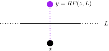
(i) (ii)

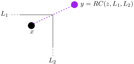
Figure 8: (i) Example of how we reflect a point with respect to a line. (ii) Example of how we reflect a point with respect to a corner.

Definition C.1 (Reflected points).

For $L\in\mathcal{L}_{\cal D}$ and $z\in{\cal D}$ we define $RP(z,L)$, the reflected point of $z$ with respect to $L$ as:

$$RP(z,L):=\{w\in{\cal D}^{c}|z-\langle z,\widehat{n}_{H_{L}}\rangle\widehat{n}_{H_{L}}=w-\langle w,\widehat{n}_{H_{L}}\rangle\widehat{n}_{H_{L}}\in L\text{ and }d(z,H_{L})=d(w,H_{L})\}.$$

For $L_{1},L_{2}\in\mathcal{P}_{\Omega}$ with $L_{1}\cap L_{2}\not=\emptyset$ we define the set of reflected points with respect to the corner, $RC(z,L_{1},L_{2})$, as:

$$RC(z,L_{1},L_{2})=\{ w\in{\cal D}^{c}|(w\not\in RP(z,L_{1})\cup RP(z,L_{2}))\wedge(\exists\widehat{z}\in RP(z,L_{2});$$

$$\widehat{z}-\langle\widehat{z},\widehat{n}_{H_{L_{1}}}\rangle\widehat{n}_{H_{L_{1}}}=w-\langle w,\widehat{n}_{H_{L_{1}}}\rangle\in\Omega^{c})\wedge(d(\widehat{z},H_{L_{1}})=d(w,H_{L_{1}}))\}.$$

We also define the ‘completed’ versions:

$$\overline{RP(z,L)}=RP(z,L)\cup\{z\},$$

$$\overline{RC(z,L_{1},L_{2})}=RC(z,L_{1},L_{2})\cup RC(z,L_{2},L_{1})\cup RP(z,L_{1})\cup RP(z,L_{2})\cup\{z\}.$$

We note that $|RP(z,L)|\leq 1$, as for any hyperplane there are two points with the same orthogonal projection and distance to it. Also we remark that for $L_{1},L_{2}\in\mathcal{L}_{\cal D}$ with $L_{1}\cap L_{2}\not=\emptyset$, and $w\in\mathbb{R}$, setting

$$\overline{RP}^{-1}(w,L_{1})=\{z\in\Omega|z\in\overline{RP}(w,L_{1})\},$$

$$\overline{RC}^{-1}(w,L_{1},L_{2})=\{z\in\Omega|z\in\overline{RC}(w,L_{1},L_{2})\},$$

for any $z\in\Omega$ we have that

$$\overline{RP}^{-1}(z,L_{1})=\overline{RC}^{-1}(z,L_{1},L_{2})=\{z\}.$$ (82)

We now define a classification of balls depending on their intersection with $\mathcal{D}$. For any $A\subset\mathbb{R}^{\mathbbm{d}}$ we set

$$A\cap\mathcal{L}_{\cal D}:=\{L\in\mathcal{L}_{\cal D}|A\cap L\not=\emptyset\text{ or }A\cap H_{L}\cap{\cal D}^{c}\not=\emptyset\}.$$

Definition C.2.

[Classification of balls in $\mathbb{R}^{2}$] Let $x\in\mathbb{R}^{2}$ and $r>0$.

1. We say $B(x,r)$ is inside ${\cal D}$ if $B(x,r)\subset{\cal D}$.

2. We say it is outside ${\cal D}$ if $B(x,r)\subset{\cal D}^{c}$.

3. We say $B(x,r)$ intersects a side of ${\cal D}$ if $|B(x,r)\cap\mathcal{L}_{\cal D}|=1$ and $B(x,r)$ is not outside of ${\cal D}$.

4. We say $B(x,r)$ intersects a corner if $|B(x,r)\cap\mathcal{L}_{\cal D}|=|\{L_{1},L_{2}\}|=2$ with $L_{1}\cap L_{2}\not=\emptyset$ and $B(x,r)$ is not outside of ${\cal D}$.

5. We say $B(x,r)$ intersects a hallway if $|B(x,r)\cap\mathcal{L}_{\cal D}|=|\{L_{1},L_{2}\}|=2$ with $L_{1}\cap L_{2}=\emptyset$ and $B(x,r)$ is not outside of ${\cal D}$.

Note that Definition C.2 provides a complete classifications of balls in $\mathbb{R}^{2}$, of radius at most $r$, given that $|B(x,r)\cap\mathcal{L}_{\cal D}|\leq 2$ for all $x\in\mathbb{R}^{2}$. With this we can define the concept of reflected sampling in $B(x,r)$.

Definition C.3 (Reflected sampling).

Let $x\in\mathbb{R}^{2}$ and $r>0$ such that $B(x,r)$ is not outside ${\cal D}$, does not intersect a hallway and $|B(x,r)\cap\mathcal{L}_{\mathcal{D}}|\leq 2$. We define the reflected sampling in $B(x,r)$ as follows:

1. If $B(x,r)$ is inside ${\cal D}$ then it is just the uniform sampling in $B(x,r)$.

2. If $B(x,r)$ intersects a side of ${\cal D}$, that is $B(x,r)\cap\mathcal{L}_{\cal D}=\{P\}$, then we pick a point $z$ uniformly at random in $B(x,r)$, take the only point in $\overline{RP}^{-1}(z,P)$.

3. If $B(x,r)$ intersects a corner of ${\cal D}$, that is $B(x,r)\cap\mathcal{L}_{\cal D}=\{L_{1},L_{2}\}$, then we pick a point $z$ uniformly at random in $B(x,r)$, then pick a point uniformly at random in $\overline{RC}^{-1}(z,L_{1},L_{2})$.

Reflected sampling can be thought of as sampling from the complete ball and then, if the ball intersects the boundary, folding it along the boundary in such a way that the content is all inside ${\cal D}$. This is illustrated for the domain $\Omega$ in Figure 9.

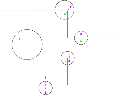
Figure 9: Reflected sampling in $\Omega$. Each of the balls intersects $\Omega$. For the ball contained completely within $\Omega$, the green point is uniformly sampled in the usual way. For balls intersecting the boundary, points in purple are sampled uniformly from the intersection of the ball with $\Omega^{c}$, corresponding to a uniformly sampled point falling outside the domain. The points in green correspond to the cases in which reflected sampling leads to a unique point within the domain. The points in yellow correspond to a case in which reflection gives two possible outcomes for the reflected sampling and we need to choose one of them uniformly at random. The purple lines join sampled points to the corresponding possible outcomes of reflected sampling.

The SLFVS on $\Omega$.

The SLFVS on $\Omega$ can now be defined in the obvious way. It is driven by the same Poisson Point Process $\Pi$ of events as in Definition 1.13, but now for a point $(t,x,r)\in\Pi$, if $B(x,r)\cap\Omega=\emptyset$ then nothing happens, and when $B(x,r)$ intersects the boundary $\partial\Omega$, parental locations are chosen according to reflected sampling, and the allele frequencies are, of course, only updated in $\Omega$. This construction will work for any domain ${\cal D}$ that fulfils the following conditions:

1. There exists a set of lines $\mathcal{L}_{\cal D}$ such that ${\cal D}$ fulfils (80) and (81).

2. There is $\mathcal{R}_{\cal D}>0$ such that, for all $x\in\mathbb{R}^{2}$, we have $|B(x,\mathcal{R}_{\cal D})\cap\mathcal{L}_{\cal D}|\leq 2$ and $B(x,\mathcal{R}_{\mathcal{D}})$ does not intersect a hallway.

3. For any $r<\mathcal{R}_{\cal D}$ and $x\in\mathbb{R}^{2}$, if $B(x,r)$ intersects a corner given by $L_{1},L_{2}$ then $\overline{RC}^{-1}(w,L_{1},L_{2})\not=\emptyset$ for all $w\in B(x,r)$. If $B(x,r)$ intersects a side given by the line $L$, then $\overline{RP}^{-1}(w,P)\not=\emptyset$ for all $w\in B(x,r)$.

We can then construct the SLFVS on ${\cal D}$, provided that events are assumed to have radius bounded by $\mathcal{R}_{{\cal D}}$. These conditions are sufficient to ensure that the reflected sampling that we use to choose a parental location will be well defined. The third condition prevents there being no pre-image through the reflection of the parental location; the second removes the possibility of an event intersecting two walls, for which we have not defined the corresponding reflected points. We could, of course, extend our definitions further, but we are primarily interested in the domain $\Omega$, and one can check that $\Omega$ fulfils these conditions with $\mathcal{R}_{\Omega}\leq r_{0}\wedge R_{0}-r_{0}$.

Blocking in the stochastic setting

Using the approach adopted in Theorem 1.17 we can prove a stochastic analogue of Theorem 1.6. While we omit the details, the key tool is a branching and coalescing dual for the SLFVS on $\Omega$. This mirrors the dual for the process on the whole Euclidean space, introduced in Definition 3.1, except that uniform sampling of offspring locations is replaced by reflected sampling.

The key ideas in the proof of Theorem 1.17 can then be adapted in the obvious way to this setting. Since we deliberately constructed the reflected sampling in such a way that transition probabilities of the jump process followed by a lineage could be obtained from those on Euclidean space via the method of images, it should be no surprise that Lemma 3.8 can be translated to this setting on replacing Brownian motion by reflected Brownian motion. The technical details will appear in the doctoral thesis of the third author.

References

- [AHM64] M. Alfaro, H. Hilhorst and H. Matano “The singular limit of the Allen–Cahn equation and the FitzHugh–Nagumo system” In J. Differ. Equ. 245.2, 1964, pp. 505–565
- [Alf+18] M. Alfaro, D. Antonopoulou, G. Karali and H. Matano “Generation of fine transition layers and their dynamics for the stochastic Allen-Cahn equation”, 2018 URL: arXiv:1812.03804v3
- [BBC16] H. Berestycki, J. Bouhours and G. Chapuisat “Front blocking and propagation in cylinders with varying cross section” In Cacl. Var. Partial Dif. 55.3, 2016, pp. 44 DOI: 10.1007/s00526-016-0962-2
- [BH91] R.. Bass and P. Hsu “Some potential theory for reflecting Brownian motion in Holder and Lipschitz domains.” In Ann. Probab. 19.2, 1991, pp. 486–508
- [Che92] X. Chen “Generation and propagation of interfaces for reaction-diffusion equations” In J. Diff. Eq. 96, 1992, pp. 116–141
- [DFL86] A. De Masi, P.. Ferrari and J.. Lebowitz “Reaction-diffusion equations for interacting particle system” In J. Stat. Phys. 44, 1986, pp. 589–644 DOI: 10.1007/BF01011311
- [EFP17] A.. Etheridge, N. Freeman and S. Penington “Branching Brownian motion, mean curvature flow and the motion of hybrid zones” In Electronic Journal of Probability 22 The Institute of Mathematical Statisticsthe Bernoulli Society, 2017
- [Eth+17] A.M. Etheridge, N. Freeman, S. Penington and D. Straulino “Branching Brownian motion and selection in the spatial -Fleming–Viot Process” In Ann. Appl. Probab. 27.5, 2017, pp. 2605–2645 DOI: 10.1007/s00208-008-0258-8
- [EV12] A.. Etheridge and A. Véber “The spatial -Fleming–Viot process on a large torus: Genealogies in the presence of recombination.” In Ann. Appl. Probab. 22.6, 2012, pp. 2165–2209 DOI: 10.1214/12-AAP842
- [EVY20] A.. Etheridge, A. Véber and F. Yu “Rescaling limits of the spatial Lambda-Fleming-Viot process with selection” In Electron. J. Probab. 25, 2020, pp. 1–89 DOI: 10.1214/20-EJP523
- [Fun95] T. Funaki “The scaling limit for a stochastic PDE and the separation of phases” In Probab. Th. Rel. Fields 102, 1995, pp. 221–288 DOI: 10.1007/BF01213390
- [Fun99] T. Funaki “Singular limit for stochastic reaction-diffusion equation and generation of random interfaces” In Acta Mathematica Sinica 15, 1999, pp. 407–438 DOI: https://doi.org/10.1007/BF02650735
- [Goo18] M. Gooding “Long term behaviour of spatial population models with heterozygous or asymmetric homozygous selection”, 2018 URL: https://ora.ox.ac.uk/objects/uuid:ef35b918-35ad-4f90-98ea-325fc692f1eb
- [HRW12] M. Hairer, M.. Ryser and H. Weber “On the triviality of the 2D Allen-Cahn equation” In Electron. J. Probab. 17.39, 2012, pp. 14
- [Lee18] K. Lee “Generation of interfaces for multi-dimensional stochastic Allen–Cahn equation with a noise smooth in space” In Stochastics 90.6 Taylor & Francis, 2018, pp. 836–860 DOI: 10.1080/17442508.2018.1426586
- [McK67] H.. McKean “Propagation of chaos for a class of non-linear parabolic equations” In Lecture Series in Differential Equations 2, 1967, pp. 177–194
- [McK75] H.. McKean “Application of Brownian motion to the equation of Kolmogorov-Petrovski-Piskunov” In Common. Pure Appl. Math. 28, 1975, pp. 323–331
- [MNL06] H. Matano, K. Nakamura and B. Lou “Periodic traveling waves in a two-dimensional cylinder with saw-toothed boundary and their homogenization limit” In Networks and Heterogeneous Media 1.4, 2006, pp. 537–568
- [Sko64] A.. Skorohod “Branching diffusion processes.” In Th. Prob. Appl. 9, 1964, pp. 492–497
- [Smy88] W.B. Smythe “Static and dynamic electricity” United States: Hemisphere Publishing., 1988
- [VW15] A. Véber and A. Wakolbinger “The spatial Lambda-Fleming–Viot process: An event-based construction and a lookdown representation” In Ann. Inst. H. Poincaré Probab. Statist. 51.2, 2015, pp. 570–598 DOI: 10.1214/13-AIHP571