Effect of interfacial spin mixing conductance on gyromagnetic ratio of Gd substituted Y₃Fe₅O₁₂

Abstract

Due to its low intrinsic damping, Y₃Fe₅O₁₂ and its substituted variations are often used for ferromagnetic layer at spin pumping experiment. Spin pumping is an interfacial spin current generation in the interface of ferromagnet and non-magnetic metal, governed by spin mixing conductance parameter $G^{\uparrow\downarrow}$. $G^{\uparrow\downarrow}$ has been shown to enhance the damping of the ferromagnetic layer. The theory suggested that the effect of $G^{\uparrow\downarrow}$ on gyromagnetic ratio only comes from its negligible imaginary part. In this article, we show that the different damping of ferrimagnetic lattices induced by $G^{\uparrow\downarrow}$ can affect the gyromagnetic ratio of Gd-substituted Y₃Fe₅O₁₂.

1 Introduction

One of the focuses of spintronics, the research area about the manipulation of spin degree of freedom, is the manipulation of magnetic moment by spin current and vice-versa [1, 2]. At magnetic interface, a spin current can be generated from a ferromagnetic layer to non-magnetic metallic layer by spin pumping [3]. The pumped spin current arises from the exchange interaction between the spin of ferromagnetic layer and the conduction spin of the non-magnetic metal [4]. The polarization of the pumped spin current depends on the dynamics of magnetic moments at the ferromagnetic layer [5]

$$\textbf{J}=\mathrm{Re}G^{\uparrow\downarrow}\textbf{m}\times\dot{\textbf{m}}-\mathrm{Im}G^{\uparrow\downarrow}\dot{\textbf{m}},$$ (1)

where m is the normalized magnetization direction and $G^{\uparrow\downarrow}$ is the interfacial spin mixing conductance [6]. While $G^{\uparrow\downarrow}$ generally has a complex value, its imaginary part is significantly smaller [7, 8].

Due to its low intrinsic damping [9, 10], Y₃Fe₅O₁₂ (YIG) [11, 12, 13] and its substituted variations[14, 15] are often used for ferromagnetic layer at spin pumping experiment. It has been observed that the spin mixing conductance can be enhanced by substituting Y in ferrimagnetic Y₃Fe₅O₁₂ with rare earths such as Gd [16, 17, 18]. Furthermore, the polarization switch of the spin current near the magnetization compensation point of Gd₃Fe₅O₁₂ is often studied [19, 20]. The magnetization compensation points occur because Gd³⁺ and Fe³⁺ ions in ferrimagnetic Gd₃Fe₅O₁₂ are antiferromagnetically coupled.

Beside using ferromagnetic resonance, spin pumping can be excited using temperature gradient $\Delta T$ and produce spin Seebeck voltage [21, 22]

$$V\propto\frac{\gamma\mathrm{Re}G^{\uparrow\downarrow}}{M_{s}}\Delta T,$$ (2)

where $\gamma$ and $M_{s}$ are the gyromagnetic ratio and saturation magnetization of ferromagnetic layer, respectively. The proportionality constant only depends on the properties of the non-magnetic metal. Ref. [14] shows that the magnitude of $G^{\uparrow\downarrow}$ at the interface of Gd-substituted Y₃ Fe₅O${}_{12}|$Pt is dominantly originated from the magnetization of Fe $G^{\uparrow\downarrow}\propto M_{\rm Fe}$. However, the linear relation of $\gamma$ and $V$ was not confirmed.

Reciprocally, spin mixing at the interface gives a torque on the magnetization in the form of spin transfer torque due to spin accumulation $\boldsymbol{\mu}_{s}$ [23].

$$\tau=\mathrm{Re}G^{\uparrow\downarrow}\textbf{m}\times\left(\textbf{m}\times\boldsymbol{\mu}_{s}\right)-\mathrm{Im}G^{\uparrow\downarrow}\textbf{m}\times\boldsymbol{\mu}_{s}$$ (3)

Spin transfer torque can be used for manipulation of the magnetization of the ferromagnetic layer [24, 25]. The real part of spin mixing conductance $\mathrm{Re}G^{\uparrow\downarrow}$ has been shown to increase the Gilbert damping of the magnetization [5].

$$\gamma\alpha=\gamma\alpha^{(0)}+M_{j}\mathrm{Re}G^{\uparrow\downarrow},$$ (4)

On the other hand, $\mathrm{Im}G^{\uparrow\downarrow}$ has been predicted to reduce the gyromagnetic ratio [4, 5].

$$\frac{1}{\gamma}=\frac{1}{\gamma^{(0)}}+M_{j}\mathrm{Im}G^{\uparrow\downarrow},$$ (5)

However, the effect of $\mathrm{Re}G^{\uparrow\downarrow}$ to the gyromagnetic ratio is not well-studied.

In this article, we aim to study the effect of $G^{\uparrow\downarrow}$ on the gyromagnetic ratio of Gd substituted Y₃Fe₅O₁₂, assuming negligible $\mathrm{Im}G^{\uparrow\downarrow}\to 0$. While $G^{\uparrow\downarrow}$ has been predicted to only increase the damping, it can also affect the gyromagnetic ratio, because the effective gyromagnetic ratio of a ferrimagnet is determined on the damping parameters of each magnetic lattice [26]. By studying the damping increase due to $G^{\uparrow\downarrow}$ of the interface in Sec. 2.1 and the coupled dynamics of two magnetic lattices in Sec. 2.2, we can describe the effect of spin mixing conductance on the effective gyromagnetic ratio of Gd substituted YIG in Sec. 3 and show that $\gamma$ in Eq. 2 should be the $G^{\uparrow\downarrow}$-corrected gyromagnetic ratio.

2 Methods

2.1 Damping torque due to interfacial spin mixing

In second quantization, the interactions of conduction spin of non-magnetic metal near the interface with $n$-th spin $\textbf{S}_{n}$ of ferromagnet layer can be written with the following $s-d$ Hamiltonian [27]

$$\mathcal{H}= \sum_{\textbf{p}\alpha}\epsilon_{\textbf{p}}a_{\textbf{p}\alpha}^{\dagger}a_{\textbf{p}\alpha}-\gamma_{e}\sum_{\textbf{p}\alpha\beta}\textbf{H}\cdot\boldsymbol{\sigma}_{\alpha\beta}a_{\textbf{p}\alpha}^{\dagger}a_{\textbf{p}\beta}$$

$$-J\sum_{n\textbf{pq}\alpha\beta}\textbf{S}_{n}\cdot\boldsymbol{\sigma}_{\alpha\beta}a_{\textbf{p}+\textbf{q}\alpha}^{\dagger}a_{\textbf{p}\beta},$$ (6)

where $\gamma_{e}$ is the gyromagnetic ratio of free electron, $a_{\textbf{p}\alpha}^{\dagger}(a_{\textbf{p}\alpha})$ is the creation (annihilation) operator of conduction electron with wave vector p and spin $\alpha$, $\boldsymbol{\sigma}$ is Pauli vectors, $\epsilon_{\textbf{p}}=\hbar^{2}p^{2}/2m$ is the energy of conduction electron and $J$ is the exchange constant.

In linear response regime, the exchange interaction dictates that the spin density of the conduction electron responds linearly to perturbation due to exchange interaction[4, 28]

$${\sigma}_{i}(\textbf{r})= \sum_{\textbf{pq}\alpha\beta}e^{i\textbf{q}\cdot\textbf{r}}\boldsymbol{\sigma}_{\alpha\beta}a_{\textbf{p}+\textbf{q}\alpha}^{\dagger}a_{\textbf{p}\beta}$$

$$= J\sum_{n}\int d\textbf{r}dt\chi_{ij}(\textbf{r}-\textbf{r}^{\prime},t-t^{\prime})S_{nj}(\textbf{r}^{\prime},t^{\prime}),$$ (7)

where $i,j\in\left\{x,y,z\right\}$. The susceptibility

$$\chi_{ij}(\textbf{r},t)= \frac{i}{\hbar}\Theta(t)\left<\left[\sigma_{i}(\textbf{r},t),\sigma_{j}(\textbf{0},0)\right]\right>$$ (8)

can be determined by evaluating its time derivation

$$\frac{\partial\chi_{ij}(\textbf{r},t)}{\partial t}=\frac{i}{\hbar}\Theta(t)\left<\left[\frac{1}{i\hbar}\left[\sigma_{i}(\textbf{r},t),\mathcal{H}_{0}\right],\sigma_{j}(\textbf{0},0)\right]\right>.$$ (9)

By setting the first two terms in Hamiltonian in Eq. 6 as the unperturbed $\mathcal{H}_{0}$, the susceptibility can be evaluated $\chi_{ij}(\textbf{r},t)=\sum_{\textbf{pq}}e^{i\textbf{q}\cdot\textbf{r}-i\omega t}\chi_{ij}(\textbf{p},\textbf{q},\omega),$ we can derive the exact expression of $\chi_{ij}$ in the static limit $\omega\to 0$ for all $i,j$ combination

$$\sum_{\textbf{p}}\left(\begin{array}[]{ccc}\chi_{xx}(\textbf{p},\textbf{q},0)&\chi_{xy}(\textbf{p},\textbf{q},0)&\chi_{xz}(\textbf{p},\textbf{q},0)\\ \chi_{yx}(\textbf{p},\textbf{q},0)&\chi_{yy}(\textbf{p},\textbf{q},0)&\chi_{yz}(\textbf{p},\textbf{q},0)\\ \chi_{zx}(\textbf{p},\textbf{q},0)&\chi_{zy}(\textbf{p},\textbf{q},0)&\chi_{zz}(\textbf{p},\textbf{q},0)\end{array}\right)$$ (13)

$$=\left(\begin{array}[]{ccc}\chi(q)&\gamma_{e}H_{z}\varphi(q)&\gamma_{e}H_{y}\varphi(q)\\ -\gamma_{e}H_{z}\varphi(q)&\chi(q)&\gamma_{e}H_{x}\varphi(q)\\ \gamma_{e}H_{y}\varphi(q)&-\gamma_{e}H_{x}\varphi(q)&\chi(q)\end{array}\right)$$ (17)

such that

$$\chi_{ij}(\textbf{r},t)= \sum_{\textbf{q}}e^{i\textbf{q}\cdot\textbf{r}-i\omega t}\sum_{\textbf{p}}\chi_{ij}(\textbf{p},\textbf{q},0)$$

$$= \delta(t)\sum_{\textbf{q}}e^{i\textbf{q}\cdot\textbf{r}}\Big{(}\delta_{ij}\chi(q)+\epsilon_{ijk}\gamma_{e}H_{k}\varphi(q)\Big{)}.$$ (18)

One can see that the susceptibility is anisotropic [29]. In the limit of small magnetic field $H\ll\epsilon_{F}$, the induced spin density takes the following form

$$\boldsymbol{\sigma}(\textbf{r})=\sum_{n\textbf{k}}e^{i\textbf{k}\cdot\textbf{r}}J\left(\chi(k)\textbf{S}_{n}+\gamma_{e}\varphi(k)\textbf{S}_{n}\times\boldsymbol{H}\right),$$ (19)

where $\chi(k)$ is the static susceptibility of a metal

$$\chi= \mathcal{N}(\epsilon_{F})\left(1+\frac{4k_{F}^{2}-q^{2}}{4k_{F}k}\log\left|\frac{k+2k_{F}}{k-2k_{F}}\right|\right)$$ (20)

and

$$\varphi(k)= \lim_{\eta\to 0}\sum_{\textbf{p}}\frac{f_{\textbf{p}}-f_{\textbf{p}+\textbf{k}}}{\left(\epsilon_{\textbf{p}+\textbf{k}}-\epsilon_{\textbf{p}}+i\eta\right)^{2}}$$

$$= \mathcal{N}^{2}(\epsilon_{F})\frac{\pi^{3}}{k_{F}^{2}\hbar}\frac{\Theta(2k_{F}-k)}{k}.$$ (21)

$\varphi$ is the anisotropic susceptibility that generates a term in $\boldsymbol{\sigma}$ that is non-collinear to $\textbf{S}_{n}$. Here $\mathcal{N}(\epsilon_{F})$ is the density of state at Fermi level. $\varphi$ term generates a spin transfer torque on spin $\textbf{S}_{n}$ [27]

$$\tau= \sum_{n}\gamma_{n}J\textbf{S}_{n}\times\boldsymbol{\sigma(\textbf{0})}$$

$$= \left(J^{2}\sum_{\textbf{k}}\varphi(k)\right)\sum_{n}\gamma_{n}\textbf{S}_{n}\times\left(\textbf{S}_{n}\times\gamma_{e}\textbf{H}\right).$$ (22)

Since $\textbf{S}_{n}=S_{n}\textbf{m}$ and $\gamma_{e}\textbf{H}$ is a spin accumulation, by comparing Eqs. 22 and 3 one can see that $\varphi$ is related to spin mixing conductance $G^{\uparrow\downarrow}=\sum_{j}G_{j}^{\uparrow\downarrow}$, where the spin mixing conductance for $j-$th lattice is

$$G_{j}^{\uparrow\downarrow}=N_{j}S_{j}^{2}J^{2}\sum_{\textbf{k}}\varphi(k),$$ (23)

where $N_{j}$ is number of spin at the interface. This torque increase the damping torque on the total magnetic moment $\textbf{M}=M_{s}V\textbf{m}$ of the whole volume of the ferromagnetic layer

$$\frac{d\textbf{M}}{dt}=\sum_{n}\gamma_{j}G_{j}^{\uparrow\downarrow}\textbf{m}\times\left(\textbf{m}\times\textbf{H}\right),$$ (24)

can be written in a normalized form

$$\frac{d\textbf{m}}{dt}=\frac{1}{M_{s}V}\sum_{n}\gamma_{j}G_{j}^{\uparrow\downarrow}\textbf{m}\times\left(\textbf{m}\times\textbf{H}\right)$$ (25)

where $M_{s}$ is magnetization saturation, $V=Ad$ is volume of the magnetic layer. One can see the damping due to spin mixing conductance is inversely proportional to thickness $d$. For YIG, Ref. [4] estimate the value per unit area to be $G_{\rm YIG}^{\uparrow\downarrow}/A\sim\textrm{\AA}^{-2}$. When Y is substituted with Gd, the spin mixing conductance should include the contributions from all magnetic lattice [30].

2.2 Landau-Lifshitz equation of ferrimagnet

The dynamics of magnetic moment of $j$-th magnetic lattice $\textbf{M}_{j}$ ($j=1,2$) in a ferrimagnet is governed by Landau-Lifshitz equation [26].

$$\frac{d\mathbf{M}_{j}}{dt}= -\gamma_{i}\mathbf{M}_{j}\times\mathbf{H}_{j}-\frac{\alpha_{j}\gamma_{j}}{M_{j}}\mathbf{M}_{j}\times\left(\mathbf{M}_{j}\times\mathbf{H}_{j}\right),$$ (26)

where $\mathbf{H}_{j}$ is the effective magnetic field felt by $\textbf{M}_{j}$ and $\alpha_{j}$ is its dimensionless damping parameter. $\textbf{H}_{j}$ consists of external magnetic field $H_{0}$ and molecular field due to coupling with another magnetic lattice

$$\textbf{H}_{j}= \textbf{H}_{0}+\lambda\textbf{M}_{k\neq j}.$$ (27)

$\lambda$ is coupling constant between magnetic lattices. The $\mathbf{M}_{j}\times\left(\mathbf{M}_{j}\times\mathbf{H}_{j}\right)$ term in Eq. 26 is the damping torque [31], that include the contribution of spin mixing conductance in Eq. 24

$$\left(\alpha_{j}-\alpha_{j}^{(0)}\right)=\frac{N_{j}G_{j}^{\uparrow\downarrow}}{M_{j}V},$$ (28)

where $N_{j}$ is number of spin at the interface, $\alpha_{j}^{(0)}$ is the intrinsic damping of $i$-th magnetic lattice of the magnetic layer. One can see the damping enhancement is inversely proportional to thickness of the ferromagnetic layer.

Here we note that the damping torque could take $\textbf{M}\times\dot{\textbf{M}}$ form as in the Landau-Lifshitz-Gilbert equation [32]. However, Ref. [33, 34] shows that Eq. 26 has better agreement with the experiment data for rare earth garnet in large damping limit, which is appropriate for spin pumping setup that has large damping.

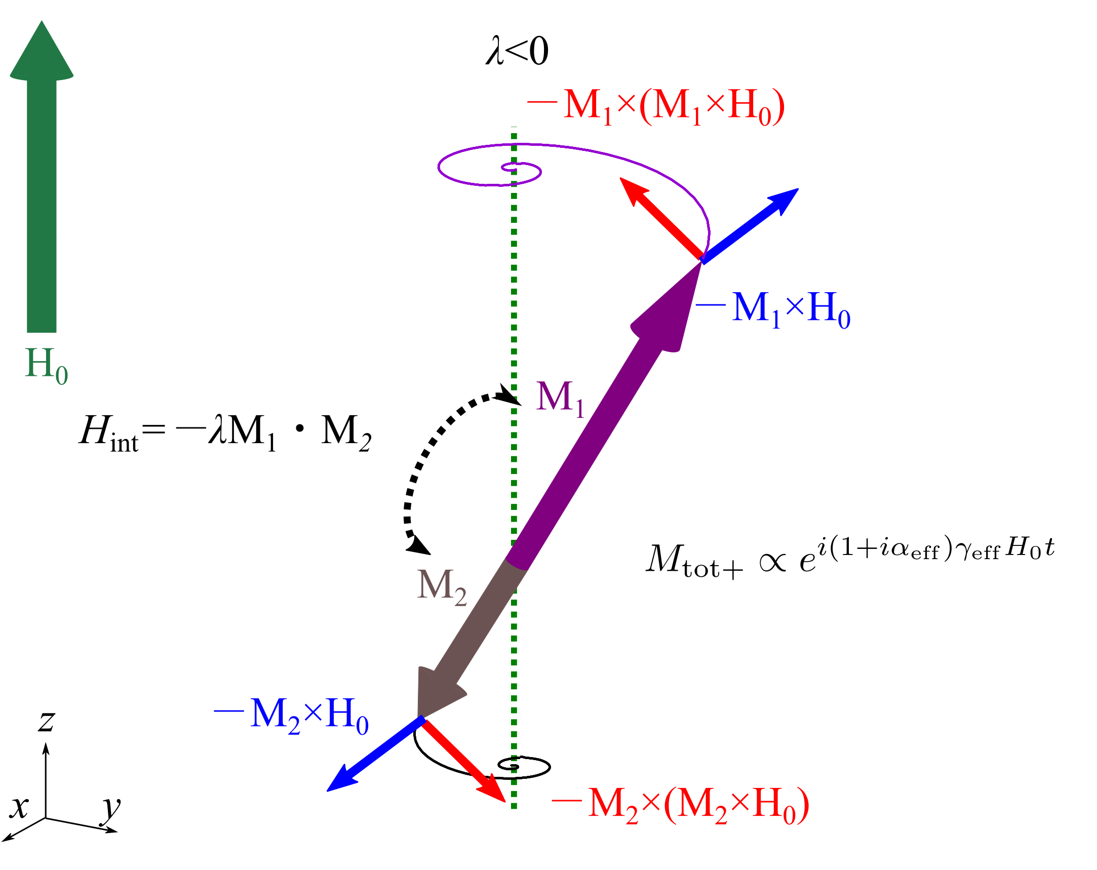
Figure 1: Ferrimagnet with two magnetic lattices $\textbf{M}_{1}$ and $\textbf{M}_{2}$ under an external magnetic field $\textbf{H}_{0}$. Due to magnetic interaction $H_{\mathrm{int}}=-\lambda\textbf{M}_{1}\cdot\textbf{M}_{2}$, the dynamics of $\textbf{M}_{1}$ and $\textbf{M}_{2}$ are coupled as a total magnetization with effective gyromagnetic ratio $\gamma_{\mathrm{eff}}$ and effective damping parameter $\alpha_{\mathrm{eff}}$. When $\lambda>0$ the coupling is ferromagnetic. On the other hand, when $\lambda<0$, the coupling is antiferromagnetic.

In the ferromagnetic resonance linear polarized microwave magnetic field is used to study the resonance spectrum of magnetic material

$$\textbf{H}_{0}=H_{0}\hat{\textbf{z}}+\hat{\textbf{x}}\delta H\cos\omega t,$$ (29)

$\delta H\ll H_{0}$. Mathematically, a linear polarized magnetic field can be written in a combination of circularly polarized magnetic field with opposite frequency

$$\hat{\textbf{x}}\cos\omega t=\frac{1}{2}\sum_{w=\pm\omega}(\hat{\textbf{x}}\cos wt+\hat{\textbf{y}}\sin wt).$$ (30)

Because of that, for mathematical simplicity, we can study the response of the magnetization dynamics of the following circularly polarized external magnetic field

$$\textbf{H}_{0}=H_{0}\hat{\textbf{z}}+(\hat{\textbf{x}}\cos\omega t+\hat{\textbf{y}}\sin\omega t)\delta H.$$ (31)

The coupled magnetization dynamics of our ferrimagnet can then be linearized by setting $M_{j+}=M_{jx}+iM_{jy}$ and assuming $M_{j+}\ll M_{jz}$. The coupled dynamics can be written in the following linear equations.

$$\frac{\partial}{\partial t}\left[\begin{array}[c]{c}M_{1+}\\ M_{2+}\end{array}\right]=iW\left[\begin{array}[c]{c}M_{1+}\\ M_{2+}\end{array}\right]-ie^{i\omega t}\delta H\left[\begin{array}[c]{c}\left(1+i\alpha_{1}\right)\gamma_{1}M_{1}\\ \left(1+i\alpha_{2}\right)\gamma_{2}M_{2}\end{array}\right]$$ (32)

where $W=$

$$\left[\begin{array}[c]{cc}\left(1+i\alpha_{1}\right)\gamma_{1}\left(H_{0}+\lambda M_{2}\right)&-\left(1+i\alpha_{1}\right)\gamma_{1}\lambda M_{1}\\ -\left(1+i\alpha_{2}\right)\gamma_{2}\lambda M_{2}&\left(1+i\alpha_{2}\right)\gamma_{2}\left(H_{0}+\lambda M_{1}\right)\end{array}\right]$$ (33)

For $\lambda\gg H_{0}$ one can show that the leading order in the eigen values of $W$ are

$$w_{1}= \lambda\left(\left(1+i\alpha_{2}\right)\gamma_{2}M_{1}+\left(1+i\alpha_{1}\right)\gamma_{1}M_{2}\right),$$ (34)

$$w_{2}= H_{0}\frac{M_{1}+M_{2}}{\frac{M_{1}}{(1+i\alpha_{1})\gamma_{1}}+\frac{M_{2}}{(1+i\alpha_{2})\gamma_{2}}}.$$ (35)

In the limit $\lambda\gg H_{0}$, the solution for $\delta H=0$ can be written as

$${M}_{\mathrm{tot}+}\propto e^{i(1+i\alpha_{\mathrm{eff}})\gamma_{\mathrm{eff}}H_{0}t},$$ (36)

as illustrated in Fig. 1. The eigenstate of $w_{2}$ determines the effective gyromagnetic ratio

$$\gamma_{\mathrm{eff}}=\frac{\mathrm{Re}w_{2}}{H_{0}}=\frac{(M_{1}+M_{2})\left(\frac{M_{1}/\gamma_{1}}{1+\alpha_{1}^{2}}+\frac{M_{2}/\gamma_{2}}{1+\alpha_{2}^{2}}\right)}{\left(\frac{M_{1}/\gamma_{1}}{1+\alpha_{1}^{2}}+\frac{M_{2}/\gamma_{2}}{1+\alpha_{2}^{2}}\right)^{2}+\left(\frac{\alpha_{1}M_{1}/\gamma_{1}}{1+\alpha_{1}^{2}}+\frac{\alpha_{2}M_{2}/\gamma_{2}}{1+\alpha_{2}^{2}}\right)^{2}}$$ (37)

and the effective damping

$$\alpha_{\mathrm{eff}}=\frac{\mathrm{Im}w_{2}}{\mathrm{Re}w_{2}}=\frac{\alpha_{1}\frac{M_{1}/\gamma_{1}}{1+\alpha_{1}^{2}}+\alpha_{2}\frac{M_{2}/\gamma_{2}}{1+\alpha_{2}^{2}}}{\frac{M_{1}/\gamma_{1}}{1+\alpha_{1}^{2}}+\frac{M_{2}/\gamma_{2}}{1+\alpha_{2}^{2}}}.$$ (38)

$\alpha_{\mathrm{eff}}$ is closely related to the width of the ferromagnetic resonance (FMR) spectrum, which can be determined from the rate of the loss of magnetic dissipation energy $\Delta F=-\textbf{H}_{0}\cdot\textbf{M}_{\mathrm{tot}}$.

$$\frac{dF}{dt}=\frac{\alpha_{\mathrm{eff}}\gamma_{\mathrm{eff}}\omega^{2}M_{\mathrm{tot}}\delta H^{2}}{\left(\omega-\mathrm{Re}w_{2}\right)+\left(\mathrm{Im}w_{2}\right)^{2}}$$ (39)

The shape of the Lorentzian function indicates that the FMR width is proportional to the effective damping parameter

$$\frac{\Delta\omega}{\omega_{\mathrm{peak}}}\sim\alpha_{\mathrm{eff}}.$$ (40)

In the limit of small $\alpha_{1},\alpha_{2}\to 0$, we get the following well-known effective gyromagnetic ratio

$$\lim_{\alpha\to 0}\gamma_{\mathrm{eff}}=\frac{M_{1}+M_{2}}{{M_{1}}/{\gamma_{1}}+{M_{2}}/{\gamma_{2}}}.$$ (41)

On the other hand, in the limit of large $\alpha_{2}\gg\alpha_{1}\approx 0$ we arrive at the Kittel gyromagnetic ratio for ferrimagnet with an overdamped $M_{2}$ [33, 35]

$$\lim_{\alpha_{2}\to\infty}\gamma_{\mathrm{eff}}=\frac{M_{1}+M_{2}}{{M_{1}}/{\gamma_{1}}}.$$ (42)

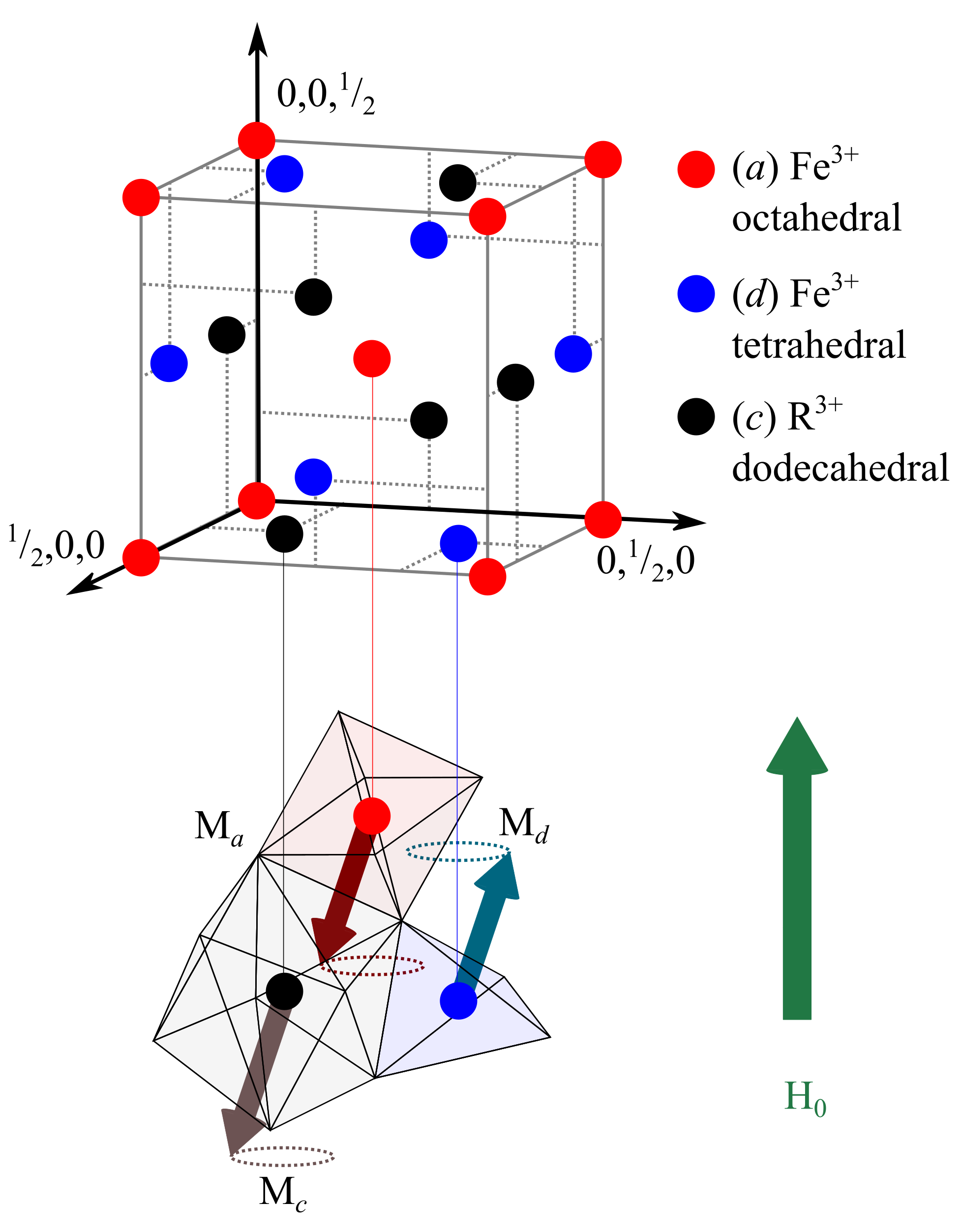
Figure 2: One eighth of a unit cell of ferrimagnetic R₃Fe₅O₁₂. Lattice constant $a=12.4$ Å. The garnet structure has metal cations (Fe³⁺ and R³⁺) and oxygen anions that form tetrahedral $(a)$, octahedral $(d)$ and dodecahedral $(c)$ sites [36, 37, 38]. R site is occupied by Y or rare earth elements and coupled antiferromagnetically with $a$-site. Fe ions occupy $a$ and $d$ sites. Because $a$ and $d$ are antiferromagnetically coupled, 4 out of 5 Fe³⁺ in R₃Fe₅O₁₂ cancel each other.

3 Results and Discussion

From here on, we focus on substituted $\mathrm{Y}_{3}\mathrm{Fe}_{5}\mathrm{O}_{12}$. It has a garnet structure that consists of tetrahedron $(d)$, octahedron $(a)$ and dodecahedron $(c)$ of oxygen ions coordinated with metal cations. The magnetic moments in tetrahedral and octahedral sites rise from Fe³⁺ ions [36]. Because $a$ and $d$ sites are antiferromagnetically coupled, 4 out of 5 Fe occupying $a$ and $d$ sites cancel each other. Y in dodecahedral site can be substituted with rare earth elements and is coupled antiferromagnetically with $a$-site as seen in Fig. 2 [36].

Ref. [14] experimentally measures the gyromagnetic ratio of Y_3-xGd_xFe_5-y(Mn,Al)_yO₁₂ for variations of $x$ and $y$. Since Gd³⁺ has non zero magnetization from half-filled 4$f$ orbital, substitution of Y creates magnetic moment at $c$ site. Mn²⁺ can substitute Fe³⁺ in $a$ site [39]. Al dominantly substitute Fe³⁺ in $d$ site when $y\leq 2$. For $y=6$%, 90% of Al³⁺ substitutes $d-$site, this percentage reduces slowly as Al percentage increases [36]. Main contribution of Mn and Al to the magnetization is the substitution of Fe in $a$ site [36]. Fig. 3 illustrates that the magnetization of substituted Y₃Fe₅O₁₂ is dominated by Fe and Gd.

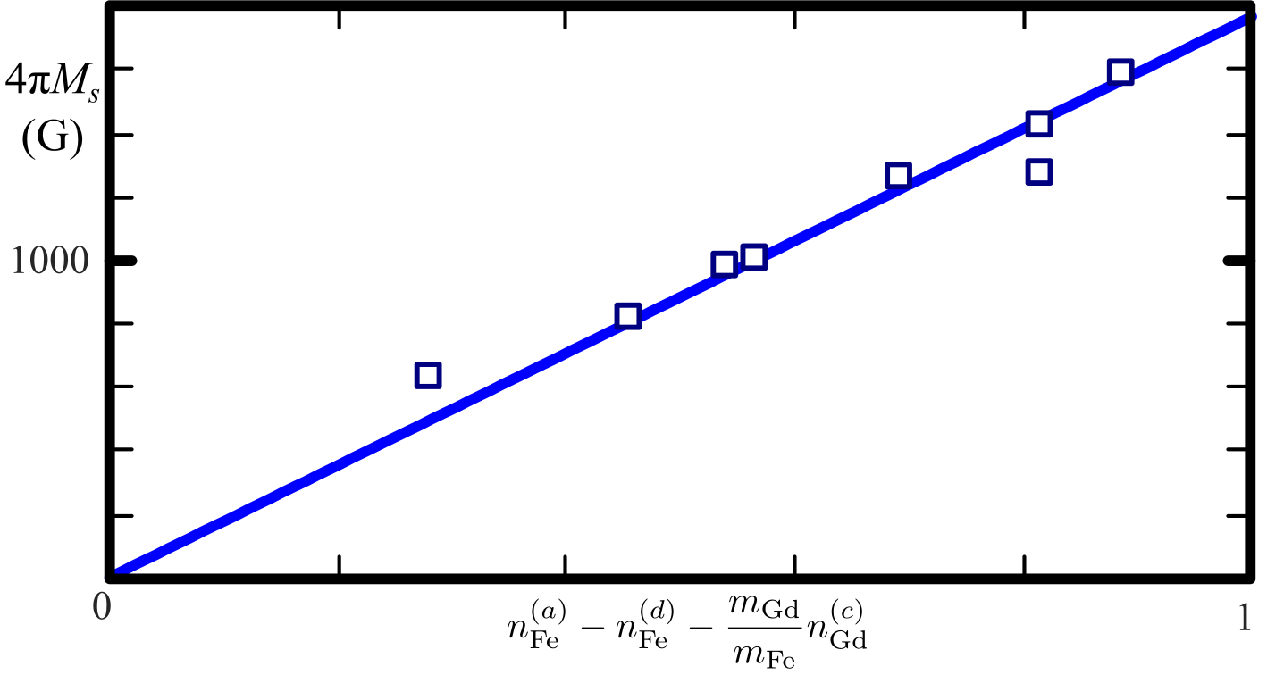
Figure 3: Magnetization of Y_3-xGd_xFe_5-y(Mn,Al)_yO₁₂ in Ref. [14] is dominated by Fe and Gd ions. Mn and Al indirectly contribute to the magnetization by substituting Fe [36]. $M_{s}$ is saturation magnetization, $m_{\rm X}$ is the magnetic moment of X ion. $n^{(j)}_{X}$ is the number of X ion at $(j)$-site. Here $m_{\rm Gd}=m_{\rm Fe}/3$.

Since magnetic moment at $d$ site cancels some of $a$ site, the magnetization of the Gd-substituted garnet arises from Fe³⁺ of $a$ site and Gd³⁺ of $c$ site. We can then set Fe³⁺ of $a$ site to be the first magnetic lattice and Gd³⁺ of $c$ site.

$$M_{1}= m_{\rm Fe}n_{\rm Fe},$$ (43)

$$M_{2}= -m_{\rm Gd}n_{\rm Gd},$$ (44)

On the other hand, $m_{\rm Gd}$ is the magnetic moment of Gd³⁺. $m_{\rm Fe}$ is the magnetic moment of Gd³⁺. Their ratio is determined by the paramagnetic response of Gd to the molecular field of Fe ion, according to Curie law [40]

$$\frac{m_{\rm Gd}}{m_{\rm Fe}}\propto\frac{1}{T}.$$ (45)

Since the compensation temperature and Curie temperature of Gd₃Fe₅O₁₂ is around 286 K [41]

$$M_{\rm Gd_{3}Fe_{5}O_{12}}= m_{\rm Fe}-3m_{\rm Gd}=0,$$ (46)

one can estimate that $m_{\rm Gd}=m_{\rm Fe}/3$.

We can now describe the trend of gyromagnetic ratio using Eq. 37. Fig. 4 illustrate the agreement of Eq. 37 with experimental data from Ref. [14]. The blue line is the gyromagnetic ratio of Y_3-xGd_x Fe_5-y(Mn,Al)_yO₁₂ bulk. From numerical fitting, one can find that

$$\alpha^{(0)}_{\rm Fe}= 0,$$ (47)

$$\alpha^{(0)}_{\rm Gd}= 0.36\pm 0.3,$$ (48)

$$\frac{\gamma_{\rm Fe}}{\gamma_{\rm Gd}}= 1.43\pm 0.10.$$ (49)

The value of $\gamma_{\rm Gd}$ can be lower than $\gamma_{\rm Fe}$ because of the crystalline field [42]. For a bilayer of Y_3-xGd_x Fe_5-y(Mn,Al)_y O₁₂ and Pt, we need to take into account the contribution of Re$G^{\uparrow\downarrow}$ according to Eq. 28.

The spin mixing conductance at the interface Y_3-xGd_x Fe_5-y(Mn,Al)_yO₁₂ and Pt increases the magnetic damping of the ferrimagnet. Since $G^{\uparrow\downarrow}_{\rm YIG}=N_{\rm Fe}G_{\rm Fe}^{\uparrow\downarrow}$ , the damping enhancement of Fe lattice is

$$\alpha_{\rm Fe}-\alpha^{(0)}_{\rm Fe}=\frac{N_{\rm Fe}G_{\rm Fe}^{\uparrow\downarrow}}{M_{\rm Fe}V}=\frac{G_{\rm YIG}^{\uparrow\downarrow}/A}{dM_{\rm YIG}}=0.95.$$ (50)

Here we used $d=1$ mm [14] and lattice constant $\sim 12$ Å. Using $G_{j}\propto S_{j}^{2}$ proportionality, the damping enhancement of Gd lattice can also be estimated

$$\Delta\alpha_{\rm Gd}= \frac{N_{\rm Gd}G^{\uparrow\downarrow}_{\rm Gd}}{M_{\rm Gd}V}=\frac{S^{2}_{\rm Gd}m_{\rm Fe}}{m_{\rm Gd}S^{2}_{\rm Fe}}\Delta\alpha_{\rm Fe}=0.22.$$ (51)

The change of damping parameter shifts the minimum value of the gyromagnetic ratio as seen in Fig. 4. Since $\gamma$ that includes spin mixing contribution is extracted from $V$ in Ref. [14] using Eq. 2 (see Appendix A), the agreement with the experiment data confirms the proportionality of $V$ and $\gamma$.

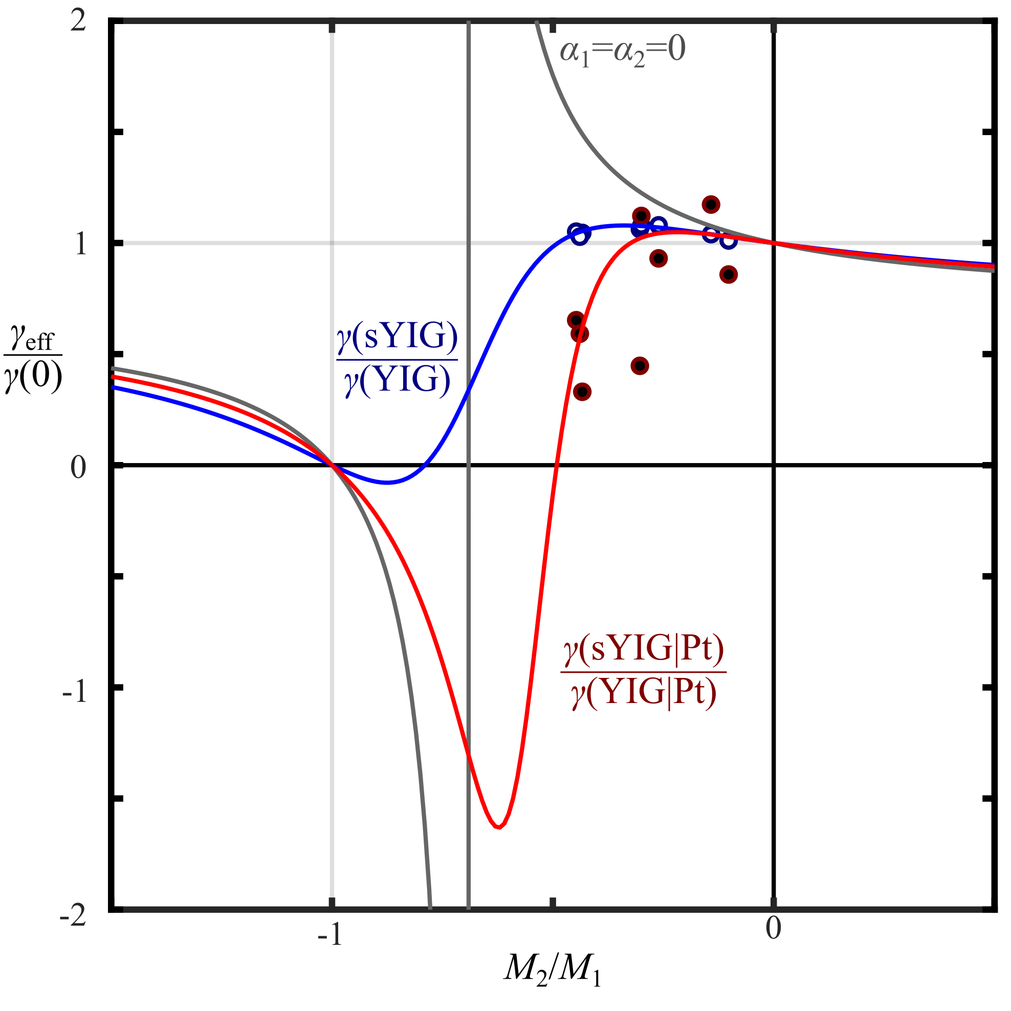
Figure 4: Normalized gyromagnetic ratio of substituted YFe₅O₁₂ (sYIG) and sYIG|Pt as a function of the ratio of $M_{1}=m_{\rm Fe}n_{\rm Fe}$ and $M_{2}=-m_{\rm Gd}n_{\rm Gd}$. The values are normalized to the value of YFe₅O₁₂ $\sim$ 1.76$\times 10^{7}$ G^-1s^-1 [43]. Negative values of $M_{2}/M_{1}$ indicate that they are antiferromagnetically coupled. Blue line is the gyromagnetic ratio of sYIG with intrinsic damping $\alpha_{\rm Fe}=0$ and $\alpha_{\rm Gd}=0.36$. Red line is the gyromagnetic ratio of sYIG|Pt with increased $\alpha_{\rm Fe}=0.95$ and $\alpha_{\rm Gd}=0.58$ due to spin mixing at the interface. Theoretical values (blue and red lines) agree with the experimental values of sYIG (white circles) and sYIG|Pt (black circles) in Ref. [14] (see Table 1). The minimum value is shifted and the width is broadened.

Table 1: Number of Gd³⁺ and Fe³⁺ that contributes to magnetization and gyromagnetic ratio of Y_3-xGd_xFe_5-y(Mn,Al)_yO₁₂ (sYIG) from Ref. [14]. The values of $\gamma_{\rm sYIG|Pt}$ are deduced from the spin Seebeck voltages (see Appendix A).

$x$	$y$	$n_{\rm Gd}$	$n_{\rm Fe}$	$\gamma_{\rm sYIG}$	$\gamma_{\rm sYIG|Pt}$
				($10^{7}$(Gs)-1)	($10^{7}$(Gs)-1)
0.69	0.628	0.65	0.50	1.84	0.58
0.72	0.218	0.70	0.77	1.87	0.79
1.11	0.208	1.10	0.82	1.85	0.15
0.40	0.102	0.40	0.94	1.83	2.06
0.90	0.092	0.86	1.10	1.90	1.64
0.31	0.018	0.30	0.98	1.78	1.51
1.35	0.018	1.33	1.01	1.81	1.04
0.91	0.006	0.89	0.99	1.90	1.97

4 Conclusion

To summarize, we discuss the effect of spin mixing conductance on the effective gyromagnetic ratio of ferrimagnetic resonance of two magnetic lattices using Landau - Lifshitz equation. We apply the two lattices model to ferrimagnetic Y_3-x Gd_xFe_5-y(Mn,Al)_yO₁₂. The two lattices model can be used for the substituted Mn and Al substitution mainly replace Fe at $a$-site, and thus the magnetization only originated from Fe and Gd. We show that it can describe the effective gyromagnetic ratio of the substituted Y₃Fe₅O₁₂ with and without Pt interface.

The interfacial spin mixing conductance influences the effective gyromagnetic ratio by increasing the damping parameter of Fe and Gd. Fig. 4 shows that the minima of gyromagnetic ratio of substituted Y₃Fe₅O₁₂ is further reduced due to spin mixing conductance of its interface with Pt. Far from the minima, the gyromagnetic ratio is weakly increased. As a comparison, the effect of small imaginary part of spin mixing conductance monotonically reduces the gyromagnetic ratio. Our result can be applied for Y₃Fe₅O₁₂ substituted by other rare earth elements which has various potential in spin-caloritonics and related areas.

DATA AVAILABILITY STATEMENTS

The authors confirm that the data supporting the findings of this study are available within the article.

Appendix A Relation of gyromagnetic ratio and spin Seebeck voltage in sYIG|Pt bilayer

Eq. 2 can be used for extracting the gyromagnetic ratio of sYIG|Pt bilayer from the spin Seebeck voltage

$$\frac{\gamma_{\rm sYIG|Pt}}{\gamma_{\rm YIG|Pt}}=\frac{\left(VM_{s}/G^{\uparrow\downarrow}\right)_{\rm sYIG|Pt}}{\left(VM_{s}/G^{\uparrow\downarrow}\right)_{\rm YIG|Pt}}.$$ (52)

From Eq. 23, one can arrive at

$$G^{\uparrow\downarrow}_{\rm sYIG|Pt}\propto n_{\rm Fe}S^{2}_{\rm Fe}+n_{\rm Gd}S^{2}_{\rm Gd}.$$ (53)

Because of that we can find the ratio

$$\frac{\gamma_{\rm sYIG|Pt}}{\gamma_{\rm YIG|Pt}}= \frac{V_{\rm sYIG|Pt}}{V_{\rm YIG|Pt}}\frac{1+\frac{m_{\rm Gd}n_{\rm Gd}}{m_{\rm Fe}n_{\rm Fe}}}{1+\frac{S^{2}_{\rm Gd}}{S^{2}_{\rm Fe}}\frac{n_{\rm Gd}}{n_{\rm Fe}}}$$

$$= \frac{V_{\rm sYIG|Pt}}{V_{\rm YIG|Pt}}\frac{1+\frac{m_{\rm Gd}n_{\rm Gd}}{m_{\rm Fe}n_{\rm Fe}}}{1+\frac{n_{\rm Gd}\left(m_{\rm Gd}/\gamma_{\rm Gd}\right)^{2}}{n_{\rm Fe}\left(m_{\rm Fe}/\gamma_{\rm Fe}\right)^{2}}},$$ (54)

which is useful for extracting $\gamma_{\rm sYIG|Pt}$ from raw spin Seebeck voltage data in Ref. [14] (see Table 2).

Table 2: Values of $n_{\rm Gd}$, $n_{\rm Fe}$, $V_{\rm sYIG|Pt}$, $\gamma_{\rm sYIG|Pt}$ extracted from Ref. [14] and the corresponding gyromagnetic ratio $\gamma_{\rm sYIG|Pt}$

$n_{\rm Gd}$	$n_{\rm Fe}$	$V_{\rm sYIG|Pt}/V_{\rm YIG|Pt}$	$\gamma_{\rm sYIG|Pt}$ ($10^{7}$(Gs)-1)
0.65	0.50	0.50	0.58
0.70	0.77	0.60	0.79
1.10	0.82	1.00	0.15
0.40	0.94	1.35	2.06
0.86	1.10	1.20	1.64
0.30	0.98	0.95	1.51
1.33	1.01	0.90	1.04
0.89	0.99	1.50	1.97

References

- Barnaś et al. [2005] J. Barnaś, A. Fert, M. Gmitra, I. Weymann, and V. K. Dugaev, Phys. Rev. B 72, 024426 (2005).
- Hirohata et al. [2020] A. Hirohata, K. Yamada, Y. Nakatani, I.-L. Prejbeanu, B. Diény, P. Pirro, and B. Hillebrands, Journal of Magnetism and Magnetic Materials 509, 166711 (2020).
- Tserkovnyak et al. [2002a] Y. Tserkovnyak, A. Brataas, and G. E. W. Bauer, Phys. Rev. B 66, 224403 (2002a).
- Cahaya et al. [2017] A. B. Cahaya, A. O. Leon, and G. E. W. Bauer, Phys. Rev. B 96, 144434 (2017).
- Tserkovnyak et al. [2002b] Y. Tserkovnyak, A. Brataas, and G. E. W. Bauer, Phys. Rev. Lett. 88, 117601 (2002b).
- Weiler et al. [2013] M. Weiler, M. Althammer, M. Schreier, J. Lotze, M. Pernpeintner, S. Meyer, H. Huebl, R. Gross, A. Kamra, J. Xiao, Y.-T. Chen, H. J. Jiao, G. E. W. Bauer, and S. T. B. Goennenwein, Phys. Rev. Lett. 111, 176601 (2013).
- Carva and Turek [2007] K. Carva and I. Turek, Phys. Rev. B 76, 104409 (2007).
- Sasage et al. [2010] K. Sasage, K. Harii, K. Ando, K. Uchida, D. Kikuchi, and E. Saitoh, Journal of Magnetism and Magnetic Materials 322, 1425 (2010).
- Chang et al. [2014] H. Chang, P. Li, W. Zhang, T. Liu, A. Hoffmann, L. Deng, and M. Wu, IEEE Magnetics Letters 5, 1 (2014).
- Serga et al. [2010] A. A. Serga, A. V. Chumak, and B. Hillebrands, Journal of Physics D: Applied Physics 43, 264002 (2010).
- Heinrich et al. [2011] B. Heinrich, C. Burrowes, E. Montoya, B. Kardasz, E. Girt, Y.-Y. Song, Y. Sun, and M. Wu, Phys. Rev. Lett. 107, 066604 (2011).
- Chen et al. [2019] Y. S. Chen, J. G. Lin, S. Y. Huang, and C. L. Chien, Phys. Rev. B 99, 220402(R) (2019).
- Burrowes and Heinrich [2012] C. Burrowes and B. Heinrich, in Topics in Applied Physics (Springer Berlin Heidelberg, 2012) pp. 129–141.
- Uchida et al. [2013] K. Uchida, T. Nonaka, T. Kikkawa, Y. Kajiwara, and E. Saitoh, Phys. Rev. B 87, 104412 (2013).
- Rosenberg et al. [2018] E. R. Rosenberg, L. c. v. Beran, C. O. Avci, C. Zeledon, B. Song, C. Gonzalez-Fuentes, J. Mendil, P. Gambardella, M. Veis, C. Garcia, G. S. D. Beach, and C. A. Ross, Phys. Rev. Materials 2, 094405 (2018).
- Geprägs et al. [2016] S. Geprägs, A. Kehlberger, F. D. Coletta, Z. Qiu, E.-J. Guo, T. Schulz, C. Mix, S. Meyer, A. Kamra, M. Althammer, H. Huebl, G. Jakob, Y. Ohnuma, H. Adachi, J. Barker, S. Maekawa, G. E. W. Bauer, E. Saitoh, R. Gross, S. T. B. Goennenwein, and M. Kläui, Nature Communications 7, 10452 (2016).
- Iwasaki et al. [2019] Y. Iwasaki, I. Takeuchi, V. Stanev, A. G. Kusne, M. Ishida, A. Kirihara, K. Ihara, R. Sawada, K. Terashima, H. Someya, K.-i. Uchida, E. Saitoh, and S. Yorozu, Scientific Reports 9, 2751 (2019).
- Ortiz et al. [2021] V. H. Ortiz, M. J. Gomez, Y. Liu, M. Aldosary, J. Shi, and R. B. Wilson, Phys. Rev. Materials 5, 074401 (2021).
- Geprägs et al. [2016] S. Geprägs, A. Kehlberger, F. D. Coletta, Z. Qiu, E.-J. Guo, T. Schulz, C. Mix, S. Meyer, A. Kamra, M. Althammer, H. Huebl, G. Jakob, Y. Ohnuma, H. Adachi, J. Barker, S. Maekawa, G. E. W. Bauer, E. Saitoh, R. Gross, S. T. B. Goennenwein, and M. Kläui, Nature Communications 7 (2016), 10.1038/ncomms10452.
- Shen [2019] K. Shen, Phys. Rev. B 99, 024417 (2019).
- Xiao et al. [2010] J. Xiao, G. E. W. Bauer, K.-c. Uchida, E. Saitoh, and S. Maekawa, Phys. Rev. B 81, 214418 (2010).
- Cahaya et al. [2015] A. B. Cahaya, O. A. Tretiakov, and G. E. W. Bauer, IEEE Transactions on Magnetics 51, 1 (2015).
- Xiao et al. [2008] J. Xiao, G. E. W. Bauer, and A. Brataas, Phys. Rev. B 77, 224419 (2008).
- Stiles and Miltat [2006] M. D. Stiles and J. Miltat, in Topics in Applied Physics (Springer Berlin Heidelberg, 2006) pp. 225–308.
- Hatami et al. [2007] M. Hatami, G. E. W. Bauer, Q. Zhang, and P. J. Kelly, Phys. Rev. Lett. 99, 066603 (2007).
- Wangsness [1958] R. K. Wangsness, Phys. Rev. 111, 813 (1958).
- Cahaya and Majidi [2021a] A. B. Cahaya and M. A. Majidi, Phys. Rev. B 103, 094420 (2021a).
- Cahaya [2021] A. B. Cahaya, Hyperfine Interactions 242 (2021), 10.1007/s10751-021-01780-0.
- Cahaya and Majidi [2021b] A. B. Cahaya and M. A. Majidi, Journal of Physics: Conference Series 1816, 012074 (2021b).
- Cahaya [2022] A. B. Cahaya, Journal of Magnetism and Magnetic Materials 553, 169248 (2022).
- Wolf [1961] W. P. Wolf, Reports on Progress in Physics 24, 212 (1961).
- Lakshmanan [2011] M. Lakshmanan, Philosophical Transactions of the Royal Society A: Mathematical, Physical and Engineering Sciences 369, 1280 (2011).
- Kittel [1960] C. Kittel, Journal of Applied Physics 31, S11 (1960), https://doi.org/10.1063/1.1984589 .
- Kittel [1959] C. Kittel, Phys. Rev. 115, 1587 (1959).
- Blume et al. [1969a] M. Blume, S. Geschwind, and Y. Yafet, Phys. Rev. 181, 478 (1969a).
- Gilleo [1980] M. Gilleo (Elsevier, 1980) pp. 1–53.
- Jain et al. [2013] A. Jain, S. P. Ong, G. Hautier, W. Chen, W. D. Richards, S. Dacek, S. Cholia, D. Gunter, D. Skinner, G. Ceder, and K. a. Persson, APL Materials 1, 011002 (2013).
- Momma and Izumi [2011] K. Momma and F. Izumi, Journal of Applied Crystallography 44, 1272 (2011).
- Geller [1960] S. Geller, Journal of Applied Physics 31, S30 (1960).
- Néel et al. [1964] L. Néel, R. Pauthenet, and B. Dreyfus (Elsevier, 1964) pp. 344–383.
- Geller et al. [1965] S. Geller, J. P. Remeika, R. C. Sherwood, H. J. Williams, and G. P. Espinosa, Phys. Rev. 137, A1034 (1965).
- Blume et al. [1969b] M. Blume, S. Geschwind, and Y. Yafet, Phys. Rev. 181, 478 (1969b).
- Förster et al. [2019] J. Förster, S. Wintz, J. Bailey, S. Finizio, E. Josten, C. Dubs, D. A. Bozhko, H. Stoll, G. Dieterle, N. Träger, J. Raabe, A. N. Slavin, M. Weigand, J. Gräfe, and G. Schütz, Journal of Applied Physics 126, 173909 (2019), https://doi.org/10.1063/1.5121013 .