Understanding temperature modulated calorimetry through studies of a model system

Abstract

Temperature Modulated calorimetry is widely used but still raises some fundamental questions. In this paper we study a model system as a test sample to address some of them. The model has a nontrivial spectrum of relaxation times. We investigate temperature modulated calorimetry at constant average temperature to precise the meaning of the frequency-dependent heat capacity, its relation with entropy production, and how such measurements can observe the aging of a glassy sample leading to a time-dependent heat capacity. The study of the Kovacs effect for an out-of-equilibrium system shows how temperature modulated calorimetry could contribute to the understanding of this memory effect. Then we compare measurements of standard scanning calorimetry and temperature-modulated calorimetry and show how the two methods are complementary because they do not observe the same features. While it can probe the time scales of energy transfers in a system, even in the limit of low frequency temperature modulated calorimetry does not probe some relaxation phenomena which can be measured by scanning calorimetry, as suggested by experiments with glasses.

I Introduction

Many calorimetry studies rely on a modulated heating power to determine a frequency-dependent heat capacity of a sample (that we henceforth call “dynamic heat capacity”) KRAFTMAKHER . There are technical reasons such as the use of a high modulation frequency so that the heat loss of the sample becomes negligible and the high accuracy which can be reached in measurements which use lock-in amplifiers and filters. There are also more fundamental motivations. Modulated techniques can be used to select among various timescales in the evolution of the system, or to determine the heat capacity while the average temperature of the sample is kept fixed and only very small oscillations are imposed. It is also an interesting method to follow the time dependence of the thermal properties of a system out of equilibrium, such as measurements on glasses. Large improvements in the experimental methods have been achieved GMELIN ; HATTA while theoretical analysis generated a lot of attention and controversy as attested by the special issue of the Journal of Thermal Analysis devoted to temperature modulated calorimetry in 1998 MENCZEL . Since then these methods are still raising some fundamental questions GARDEN-REVIEW to understand the meaning of the measurements SCHAWE ; READING1997 which are sometimes described by a complex specific heat. The puzzle becomes even more complicated when relaxation phenomena in the sample are mixed with its response to a modulated heat signal ANDROSCH ; TOMBARI2007 .

Theoretical analyses from irreversible thermodynamics GARDEN-REVIEW or linear response theory NIELSEN bring useful insights, but these approaches could be usefully completed by the investigation of a system which can be fully characterized and controlled. One feature which characterizes physics is that it has often made progress by studying simple “model” systems, whether they are real systems such as the hydrogen atom in the development of quantum mechanics or theoretical models such as the Ising model for statistical physics. At a first glance they may appear as too simple, but, because they allowed physicists to identify the basic mechanisms behind the observations, they turned out to provide elements for a basic understanding. Moreover some of the simplest theoretical models such as the Ising model can even be applied to quantitatively describe a large variety of real systems to a good approximation. In this paper we show how a simple thermodynamic model can clarify many questions which arise in the analysis of modulated calorimetry experiments.

To be useful such a model should be sufficiently simple to allow a complete analysis, but nevertheless rich enough to capture subtle effects which appear in real experimental situations. The idea to investigate the properties of a model system to clarify the meaning of the dynamic heat capacity has already been explored in the study of a bead-spring chain viewed as a model for a glass former BROWN-JR2009 ; BROWN-JR2011 however this system is too complex to allow a full analytical analysis. Recently we showed that a three-state system can play the role of the “simplest complex system” able to describe a large variety of properties of glassy systems, for instance the subtle Kovacs effect which demonstrates that thermodynamic variables are not sufficient to characterize the state of some out-of-equilibrium systems such as glasses, while allowing an analytical analysis of most of the phenomena PG . In this paper we show that this model can also provide a useful test system to investigate the different contributions which enter in the signal measured in a temperature modulated calorimetry experiment and to relate them to the underlying physical phenomena. However we want to stress that, in the context of this paper, the model is only a convenient tool for our analysis because it describes a system in which energy transfers occur at various time scales. This is the class of phenomena which are typically studied by temperature-modulated calorimetry. The possibility to derive analytical expressions for the response of this system, even when it is very far from equilibrium and shows strong relaxations, clarifies the origin of the different contributions which can be detected with temperature-modulated calorimetry and should hopefully help in the analysis of experimental data for various systems.

Section  II introduces the three-state model which is at the basis of this study and discusses its application to numerical simulations of temperature modulated calorimetry experiments. Section III analyzes temperature modulated calorimetry experiments carried at constant average temperature, starting from the determination of the dynamic specific heat for an equilibrium state and then studying out-of-equilibrium states reached after a temperature jump. We show that a full analytical treatment is possible in these cases so that the different contributions to the signal recorded in the measurements can be precisely assigned. This brings further light on the meaning of the frequency-dependent specific heat beyond the linear response theoryNIELSEN and the origin of the influence of temperature modulation on the properties of some systems, which has been observed experimentally JOHARI1999 . Section IV considers experiments in which a modulation is superimposed to a temperature ramp, as in Modulated Temperature Scanning Calorimetry (MTSC). Experiments detect a qualitative difference between the specific heat recorded in a standard Differential Scanning Calorimetry (DSC) experiment, which uses the ramp alone, and the frequency-dependent specific heat obtained by MTSC LAARRAJ . They can be understood from simulations and analytical calculations using the three-state model. Section V is a concluding discussion of the meaning of our results and their interest to analyze the data of temperature modulated calorimetry on real systems.

II The model and its application in calorimetry

The thermodynamic properties of complex systems can be approximately described by models which focus on the minima of their free energy landscape STILLINGER-82 . If this picture is completed by the values of the barriers between the minima, dynamical properties can also be investigated. Pushing these idea to the extreme leads to the two-level system, which is able to describe some surprising features of glasses. For instance, in a glass which has been cooled very fast, some degrees of freedom are trapped in high energy metastable states due to kinetic constraints. Then, upon heating those states may relax so that, in a first stage, the energy decreases while temperature increases, which is detected as a negative heat capacity in the measurements BISQUERT . The two-level system is able to describe this phenomenon, observed for instance in $\mathrm{B_{2}O_{3}}$ DEBOLT . However such an oversimplified system is not able to describe more subtle properties of glasses, such as the Kovacs effect which demonstrates that an out-of-equilibrium system is not fully characterized by the knowledge of its thermodynamic variables PG . Adding one metastable state to get the three-state system shown on Fig. 1 is enough to describe such a phenomenon. Moreover the three-state system is interesting in the context of temperature modulated calorimetry because the spectrum of its relaxation times has two characteristic times instead of the single relaxation time of the two-level system. Therefore its dynamics is richer and can exhibit non trivial time-dependencies beyond a simple exponential relaxation. The Kovacs effects is only an example of such a situation PG .

Of course a model which only considers the minima of the free energy landscape cannot be complete. It only describes the configurational heat capacity because it ignores other contributions to the energy, such as the vibrational or electronic contributions. However, for glasses, the configurational heat capacity is strongly dominant, as shown for instance by measurements on poly(vynil acetate) (PVAC) TOMBARI2007 .

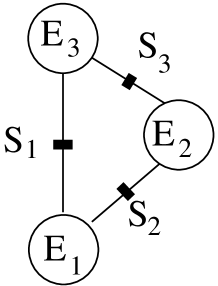
Figure 1: The three-state model. The circles schematize the metastable states with energies $E_{i}$ and the thick lines the barriers that separate them, with energies $S_{i}$.

Let us denote by $E_{i}$ ($i=1,2,3$) the energies of the three metastable states. The probabilities $P_{i}$ that the states $i$ are occupied are the variables which define the state of the system. However, due to the constraint $P_{1}+P_{2}+P_{3}=1$, the state is actually defined by two parameters only. The two variables $P_{1}$ and $P_{2}$ are sufficient to characterize a state of the system.

The equilibrium properties of the model are readily obtained from the Gibbs canonical distribution. Its partition function is

$$Z=\sum_{i}e^{-E_{i}/T}\;,$$ (1)

if we measure the temperature $T$ in energy units (which is equivalent to setting the Boltzmann constant to $k_{B}=1$). When the system is in equilibrium the occupation probabilities of the three states are

$$P_{i}^{\mathrm{eq}}=\frac{1}{Z}e^{-E_{i}/T}\;,$$ (2)

the average energy of the system is

$$E^{\mathrm{eq}}(T)=\langle E(T)\rangle^{\mathrm{eq}}=\frac{1}{Z}\;\sum_{i}E_{i}e^{-E_{i}/T}\;,$$ (3)

and its equlibrium heat capacity is

$$C^{\mathrm{eq}}(T)=\frac{dE^{\mathrm{eq}}(T)}{dT}=\frac{1}{T^{2}}\left[\langle E^{2}(T)\rangle^{\mathrm{eq}}-\Big{(}\langle E(T)\rangle^{\mathrm{eq}}\Big{)}^{2}\right]\;,$$ (4)

where $\langle\;\rangle^{\mathrm{eq}}$ designates averages computed with the equilibrium probabilities (Eq. (2) ). Viewing this model as a simplified picture of the free energy landscape of a glass, we assume that the transitions from one basin of attraction to another are thermally activated over saddle points having energies $S_{1}$, for the transition between $E_{1}$ and $E_{3}$, $S_{2}$ for the transition between $E_{1}$ and $E_{2}$, and $S_{3}$ for the transition between $E_{2}$ and $E_{3}$. Therefore the transition probabilities are determined by a set barriers $B_{ij}$, for instance $B_{13}=S_{1}-E_{1}$, $B_{31}=S_{1}-E_{3}$, $B_{12}=S_{2}-E_{1}$, and so on. The energies of the saddle points are assumed to be higher than the energies of the states that they separate so that $B_{ij}>0$ for all $i,j$ pairs.

The rates of the thermally activated transitions are

$$W_{i\to j}=\omega_{ij}\;e^{-B_{ij}/T}$$ (5)

where $\omega_{ij}$ are model parameters which have the dimension of inverse time. As a result the thermodynamics of the model is expressed by equations for the time-dependence of the occupation probabilities, which are of the form

$$\frac{dP_{1}}{dt}= -P_{1}\,\omega_{13}\,e^{-(S_{1}-E_{1})/T}+P_{3}\,\omega_{31}\,e^{-(S_{1}-E_{3})/T}$$

$$-P_{1}\,\omega_{12}\,e^{-(S_{2}-E_{1})/T}+P_{2}\,\omega_{21}\,e^{-(S_{2}-E_{2})/T}\;,$$ (6)

and similar equations for $P_{2}$ and $P_{3}$. The detailed balance conditions $\omega_{ij}=\omega_{ji}$ ensure the existence of the equilibrium state. Detailed balance does not require $\omega_{13}=\omega_{12}$, however we shall henceforth assume

$$\omega_{ij}=1\qquad\forall i,j(i\not=j)\;.$$ (7)

Setting the common value of $\omega_{ij}$ to $1$ defines the time unit (t.u.) for the system.

In a typical temperature modulated calorimetry experiment a physical system of interest, the sample, is linked by a heat exchange coefficient $K$ to a thermal bath at temperature $T_{0}$ (which could be time dependent if a thermal ramp is used). An oscillatory power is transmitted to the sample, causing its temperature to oscillate. Temperature and energy flow exchanged by the sample and its environment are monitored so that the variation of its temperature and energy versus time are known, allowing a determination of its heat capacity. Our simulations use a simpler scheme, which is adapted for a theoretical investigation. We impose the temperature $T(t)$ of the sample as a function of time. Given an initial state, this allows us to solve the equations for the time dependence of the occupation probabilities of the three states with a fourth order Runge-Kutta scheme, so that the energy $E(t)$ is determined.

While the goal of calorimetry is to relate the variations of the energy and temperature in a physical system, in temperature modulated calorimetry experiments the energy is generally controlled through the modulated power applied to the sample, and temperature is measured. In our case the situation is reversed because temperature is controlled and energy is measured (or rather calculated). In both cases the heat capacity can be deduced from the relation between energy and temperature but our simulations cannot claim to address all the phenomena which take place in an actual calorimetry experiment. In a complex system, including the three-state system, knowing the energy does not fully determine the state of the system because several configurations can lead to the same energy. One question which could be asked is how does the energy split between the microscopic degrees of freedom. Temperature Modulated calorimetry can try to answer this question by measuring the response to different modulation frequencies, which is determined by the physical processes which take place in the system and govern the energy exchange between microscopic states. In the three-state system the energy exchanges are imposed by the variations of temperature that we impose and by the rules that define the transition probabilities between states. Nevertheless, as far as the calorimetric measurements are concerned, our studies can probe how the calorimetric signal is affected, given the different time scales determined by the temperature of the system.

III Temperature Modulated calorimetry at constant average temperature

In this section we consider a sample, modeled by the three-state system, with a modulated temperature

$$T(t)=T_{0}+T_{\mathrm{ac}}(t)\quad{\mathrm{with~{}~{}}}T_{\mathrm{ac}}(t)=A_{T}\sin\omega t$$ (8)

where $T_{0}$ is a constant. This may occur in various experimental situations. (i) If the system is in equilibrium at temperature $T_{0}$, adding a small modulation ($A_{T}\ll T_{0}$) allows the measurement of its response at different frequencies to probe the spectrum of the thermal relaxations of the sample. (ii) If the system is strongly out-of-equilibrium at the start of the experiment, one may be interested in its thermal aging, i.e. the time evolution of its heat capacity $C(T_{0},t)$. Some temperature change is necessary to measure the thermal response. Choosing a temperature modulation $T_{\mathrm{ac}}(t)$ has a double interest. First the average temperature of the sample is not modified so that, if $A_{T}\ll T_{0}$ one measures the specific heat at $T_{0}$ to a good accuracy, and second, as the measurement depends on $\omega$, the time dependence of the dominant relaxation phenomena within the sample can be followed. (iii) If $A_{T}$ is large, nonlinearities are excited and we shall show that this can lead to some relaxation even if the system starts from an equilibrium state, as observed in some experimental investigations WANG-JOHARI .

III.1 Spectrum of the fluctuations of energy transfers in an equilibrium system

Using the three-state system as a “sample” we can simulate a temperature modulated calorimetry experiment that probes the time scales at which the energy can be transferred between the degrees of freedom of a physical system.

In these calculations we used the following parameters: The energies of the three metastable states are $E_{1}=-0.40$, $E_{2}=-0.25$, $E_{3}=0$. The energies of the saddle points are $S_{1}=0.40$ between states 1 and 3, $S_{2}=0.30$ between states 1 and 2, $S_{3}=0.25$ between states 2 and 3 (Fig. 1). As the model has not been tailored to any particular physical system, the energy scale is irrelevant and the values have been chosen arbitrarily. Temperatures are measured in energy units. Other values would of course quantitatively change the results, but, as long as the barriers $S_{j}-E_{i}$ for all the possible transitions are positive and the ratios of the investigated temperatures and energies stay in the same range, the main features of the results would not be affected.

Figure 2: Equilibrium heat capacity (dashed line) and equilibrium energy (full line) versus temperature (in energy units) for the three-state model with $E_{1}=-0.40$, $E_{2}=-0.25$, $E_{3}=0$ and $S_{1}=0.40$, $S_{2}=0.30$, $S_{3}=0.25$.

Figure 2 shows the equilibrium heat capacity and the equilibrium energy of the model versus temperature for this parameter set. A temperature modulated calorimetry measurement is simulated by imposing a variation of $T(t)$ according to Eq. (8) and solving the equation (II) and the similar equation for $P_{2}$ (and $P_{3}=1-P_{1}-P_{2}$ is then obtained too) with a 4th order Runge-Kutta algorithm, using the time step $\delta t=0.01$. We have chosen $T_{0}=0.125$ and, in this section, the initial state is the equilibrium state at $T=T_{0}$. Therefore, at this stage, no aging phenomena are involved.

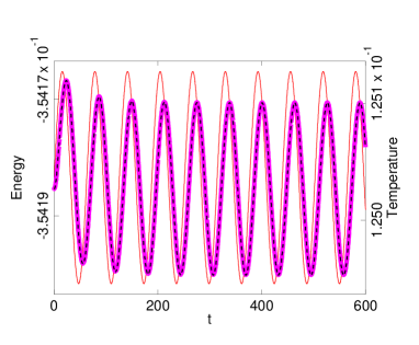
Figure 3: Energy and temperature versus time recorded in a simulation of the three state system, starting from an equilibrium state at temperature $T_{0}=0.125$, subjected to a modulated temperature according to Eq. (8) with $\omega=0.1$, $A_{T}=10^{-4}$. The thin red curve shows $T(t)$ (right scale) and the thick magenta line shows the energy recorded in the numerical simulation (left scale). The dashed black line shows the energy $E(t)$ calculated analytically (Appendix A).

Figure 3 shows a typical simulation result, for $\omega=0.1$ and $A_{T}=10^{-4}$ chosen so that the magnitude of the temperature modulation is much smaller that $T_{0}$, as in actual temperature modulated calorimetry experiments. After a short transient, discussed below, the system reaches a steady state in which the energy oscillates, with a phase shift with respect to the temperature modulation.

The heat capacity of the system $C(\omega,t)=dE/dT$ can be derived from the simulation results $C(\omega,t)=[dE(t)/dt]\,/\,[dT(t)/dt]$. Separating the fraction of $dE(t)/dt$ which is in phase with $dT(t)/dt$ one gets $C^{\prime}(\omega,t)$ while the fraction in quadrature with $dT(t)/dt$ gives $C^{\prime\prime}(\omega,t)$, which correspond to the “real” and “imaginary” parts of $C(\omega,t)$ when one uses a complex notation.

However, for the three-state system, $C(\omega,t)$ can also be calculated analytically, as shown in Appendices A and B, which gives a much better insight into the actual mechanisms which contribute to the dynamic specific heat. As the amplitude of the temperature modulation is small, the rates of the thermally activated transitions can be expanded to first order around their values at temperature $T_{0}$. It is convenient to introduce the deviations $Q_{i}(t)=P_{i}(t)-P_{i}^{\mathrm{eq}}(T_{0})$. In the general case these deviations are not assumed to be small because the calculation also applies for instance when we study a system which has been brought to $T_{0}$ after a large temperature jump. The analytical solution amounts to solving a set of two coupled equations for $dQ_{1}/dt$ and $dQ_{2}/dt$ which derive from Eq. (II) and from the corresponding equation for $dP_{2}/dt$. The two equations can be written in a matrix form and the solution is expressed on the basis of the two eigenstates of the $2\times 2$ matrix which relates the $Q_{i}$s and their time derivatives. Each eigenmode has a relaxation time $\tau_{i}$ so that the calculation shows that the dynamics of the model is governed by two relaxation times $\tau_{1}$ and $\tau_{2}$, which depend on temperature. Figure 4 shows how the relaxation times depend on temperature for the parameter set that we have chosen. In the high temperature limit the rates of the transitions tend to unity according to Eq. (5), with the time unit defined by setting $\omega_{ij}=1$, whereas, in the low temperature range, $T\lesssim 0.03$, $\tau_{1}$ and $\tau_{2}$ grow by many orders of magnitude in a narrow temperature range so that the three-state system exhibits a glass-like behavior although it does not have a true glass transition.

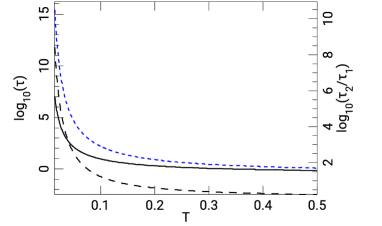
Figure 4: Relaxation times $\tau_{1}$ (black full line) and $\tau_{2}$ (blue dotted line) versus temperature, and the ratio $\tau_{2}/\tau_{1}$ (black dashed line). The relaxation times are measured in the time unit defined by setting the prefactors $\omega_{ij}=1$ in Eq. (5).

At $T_{0}=0.125$ the relaxation times are $\tau_{1}=5.217\;$t.u. and $\tau_{2}=49.11\;$t.u. corresponding to eigenfrequencies $\omega_{1}=1.204\,$t.u.^-1 and $\omega_{2}=0.1279\,$t.u.^-1. The dashed black line on Fig. 3 shows the analytical result for $E(t)$. It exactly matches the magenta line showing the energy $E(t)$ deduced from the numerical simulation, which indicates that the linear expansion of the reaction rates is sufficient to accurately describe the dynamics of the system. The agreement remains very good even if $A_{T}$ is increased by one order of magnitude to $A_{T}=10^{-3}$.

After the initial transient the energy reaches a steady oscillatory state and the heat capacity depends on $\omega$ only. Temperature Modulated calorimetry can get access to the spectrum of the characteristic times of the energy transfers within the degrees of freedom of sample by carrying a series of experiments with different modulation frequencies. For the three-state model that spectrum is known because the analytical calculation determines the two relaxation times $\tau_{1}$, $\tau_{2}$ and how they influence the specific heat because it gives the functional form of $C^{\prime}(\omega)$ and $C^{\prime\prime}(\omega)$, plotted on Fig. 5 for the model parameters that we have chosen. This figure also shows individual points, deduced from a series of numerical simulations with different values of $\omega$. They illustrate how one would build the curves for $C^{\prime}(\omega)$ and $C^{\prime\prime}(\omega)$ in a series of experiments.

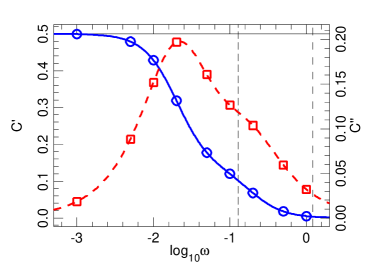
Figure 5: Heat capacities $C^{\prime}(\omega)$ (blue full line) and $C^{\prime\prime}(\omega)$ (red dashed line) for the three-state system with the parameters that we have chosen, at temperature $T_{0}=0.125$. The lines result from the analytical calculations (Appendices A and B). The points have been obtained from numerical simulations for different values of $\omega$. The vertical dashed lines show the values of $\omega_{1}$ (long dash) and $\omega_{2}$ (short dash). The black horizontal line near the top of the graph shows the value of the equilibrium heat capacity at temperature $T_{0}$ on the scale of $C^{\prime}$.

The shape of the curves shows how the eigenfrequencies play the role of cutoff frequencies for energy transfer. Above the highest frequency none of the modes can be excited and $C(\omega)$ quickly drops to $0$. In the frequency range $\omega_{2}<\omega<\omega_{1}$ one of the two modes can still be excited and therefore $C(\omega)$ still keeps a significant value. At very low frequency, as expected $C^{\prime}(\omega)$ tends to the equilibrium heat capacity while $C^{\prime\prime}(\omega)$ tends to vanish.

The physical meaning of the frequency-dependent heat capacity has been widely discussed in the literature GARDEN-REVIEW , and particularly its so called “imaginary part”, which appears as linked to some form of heat dissipation. It actually describes the component of the response which is in quadrature of phase with the temperature modulation due to delays caused by energy transfers between the various energy states. Using the three-state model the origin of this contribution to the heat capacity can be related to the entropy production in an out-of-equilibrium system. In a thermodynamic transformation, the variation $\Delta S$ of the entropy includes two contributions. The contribution $\Delta_{\mathrm{e}}S=\Delta E/T$ comes from the exchange of energy $\Delta E$ with the environment. The second contribution $\Delta_{\mathrm{i}}S$ is associated to internal transformations within the system. It is never negative $\Delta_{\mathrm{i}}S\geq 0$ and vanishes for a reversible process. For the three-state system, both simulations and analytical calculations can determine the time evolution of the probabilities of occupation of the metastable states $P_{i}(t)$, which were used in the calculation of $C(\omega)$. Therefore we can calculate the entropy of the system

$$S(t)=-\sum_{i=1}^{3}P_{i}(t)\;\ln P_{i}(t)\;.$$ (9)

The variation of entropy in an elementary transformation in which the probabilities of occupation change by $dP_{i}$ is therefore $dS=-\sum_{i=1}^{3}\ln P_{i}\;dP_{i}$ (taking into account $\sum dP_{i}=0$). $d_{\mathrm{e}}S=(1/T)\sum_{i=1}^{3}E_{i}\;dP_{i}$ can be expressed in terms of the equilibrium occupation probabilities at temperature $T$ as $d_{\mathrm{e}}S=-\sum_{i=1}^{3}\ln P^{\mathrm{eq}}_{i}\;dP_{i}$ so that the entropy production rate is

$$\mathcal{A}_{S}=\frac{d_{\mathrm{i}}S(t)}{dt}=\frac{dS(t)}{dt}-\frac{d_{\mathrm{e}}S(t)}{dt}=-\sum_{i=1}^{3}\ln\left(\frac{P_{i}}{P^{\mathrm{eq}}_{i}}\right)\frac{dP_{i}}{dt}\;.$$ (10)

It is shown in Fig. 6 for the transformation shown in Fig. 3 during which a temperature modulation is applied to the three-state system initially in equilibrium at $T=0.125$. The entropy production rate is very small (its maximum is of the order of $8\,10^{-9}$ while the entropy is of the order of $6\,10^{-1}$) but nevertheless non-zero, and always positive as expected. It shows two peaks per period of the temperature modulation, one when energy rises and one when it decreases. It simply means that the modulation of the temperature is too fast to allow the system to stay in equilibrium when temperature and energy change (whatever the change, positive or negative) and this leads to entropy production. These out-of-equilibrium processes are responsible for the $C^{\prime\prime}(\omega)$ term in the heat capacity, which has been described as a “loss term” in some studies GARDEN-REVIEW . The frequency dependence of the maximum of the entropy production rate, which rises to $2\,10^{-8}$ for $\omega=1.0\,$t.u.^-1 and drops to $1.2\,10^{-11}$ for $\omega=10^{-3}\,$t.u.^-1 attests of the role of out-of-equilibrium phenomena in a temperature modulated calorimetry experiment.

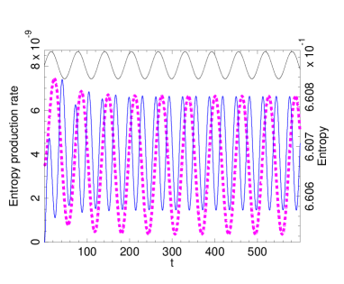
Figure 6: Entropy $S(t)$ (magenta dashed line, right scale) and entropy production rate $\mathcal{A}_{S}$ (blue full line, left scale) for the numerical experiment shown in Fig. 3. The sinusoidal function on top shows the variation of the temperature as a phase reference (no scale).

Up to now we discussed the steady state of the simulated experiment (Fig. 3). However the simulation shows a small decay of the average energy before this steady state is reached, and this may seem surprising because we started from an equilibrium state at temperature $T_{0}$ and imposed a small sinusoidal temperature modulation around $T_{0}$. Therefore the average temperature has been maintained at $T=T_{0}$. Actually the energy shift, due to this modulation is easy to understand by looking at the curve showing how the equilibrium energy $E^{\mathrm{eq}}(T)$ varies versus the temperature of the system (Fig. 2). Around $T_{0}=0.125$, $E^{\mathrm{eq}}(T)$ varies non-linearly versus temperature and is curved downwards. As a result, for a system oscillating along this curve between $T_{0}-A_{T}$ and $T_{0}+A_{T}$ the average energy is expected to be smaller than $E^{\mathrm{eq}}(T_{0})$. This simple qualitative explanation can be checked by performing a similar simulation at a temperature $T^{\prime}_{0}$ around which $E^{\mathrm{eq}}(T)$ is curved upwards. This is the case for $T^{\prime}_{0}=0.05$ as shown in Fig. 2 and indeed a simulation shows that the average energy moves up when a sinusoidal modulation of the temperature around $T^{\prime}_{0}$ is imposed. Of course, as discussed above, the system subjected to such a sinusoidal modulation is not in equilibrium. Thus the equilibrium $E^{\mathrm{eq}}(T)$ cannot provide an accurate evaluation of the average energy shift in the presence of the modulation $T_{\mathrm{ac}}$. To get such an evaluation one has to calculate the actual evolution of the energy versus time, as in Appendix A, which is plotted as a dashed black line in Fig. 3. The figure shows that this analytical calculation matches the simulation results (thick magenta line on Fig. 3). The role of a sinusoidal temperature modulation to modify the average value of some property of a material has already been observed experimentally JOHARI1999 for the dielectric relaxation and thermodynamic properties of polymers. The understanding of these phenomena, further refined in WANG-JOHARI involves exactly the same mechanism that we exhibited for the three-state system: the nonlinear change of this property when temperature varies. In some cases experiments show that the effect can become large, and this is also the case for the three-state model around $T_{0}=0.04$ because, below this temperature $E^{\mathrm{eq}}(T)$ becomes almost flat, while above $T_{0}=0.04$ it starts to raise significantly. In this temperature range the calculation of Appendix A loses accuracy because expanding the rates of the thermally activated transitions to first order in $T_{\mathrm{ac}}$ is not enough. Higher order terms, introducing further nonlinearities, start to play a significant role.

III.2 Time-dependent heat capacity during the aging of a sample at constant temperature

Understanding aging in glasses is a challenge for theoretical physics. Experiments are generally made by following the properties of a glass while it is cooled fast enough to prevent it from reaching equilibrium. In this case aging results from the combined effect of the temperature change and intrinsic phenomena within the glass. This makes the analysis more complex. Using a modulated temperature as in Eq. (8) allows measurements of thermodynamic properties while the glass ages at constant temperature because $T_{\mathrm{ac}}\ll T_{0}$ can be chosen so small that it has a negligible influence on the aging. Moreover $\omega$ can be varied to follow specific time scales during aging. The three-state system, which has a spectrum of fluctuations which is richer than a simple relaxation, is a interesting case to study how aging can lead to a time dependent heat capacity of a glass during aging.

(a)

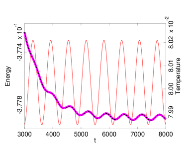
(b)

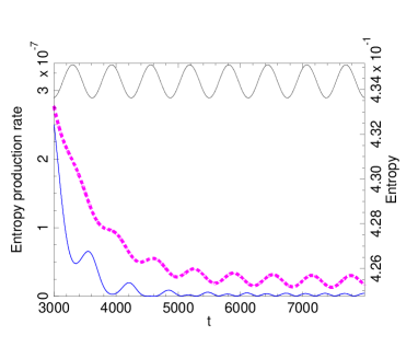
Figure 7: Time evolution of the thermodynamic properties of the three-state system during aging at $T_{0}=0.08$, with a modulation $T_{\mathrm{ac}}=A_{T}\sin\omega t$ ($\omega=10^{-2}\,$t.u.^-1, $A_{T}=2\,10^{-4}$) after a temperature jump from equilibrium at $T=0.3$. (a) Energy (thick magenta full line from simulation results, dotted black line from analytical calculation - left scale) and temperature (thin red full line, right scale). (b) Entropy (magenta dashed line, right scale) and entropy production rate (blue full line, left scale). The sinusoidal curve shows temperature as a reference (scale not indicated).

Figure 7 shows the behavior of energy, entropy, and entropy production during the early stage of aging of the three-state system after a temperature jump. In this simulation the model studied above (with the same parameters) was kept in equilibrium at $T=0.3$ for a short time and then its temperature was abruptly changed to $T_{0}=0.08$ while we followed its properties by adding a small modulation with frequency $\omega=10^{-2}\,$t.u.^-1 and amplitude $A_{T}=2\,10^{-4}$. At $T_{0}=0.08$ the relaxation times are $\tau_{1}=19.09\;$t.u. ($\omega_{1}=0.329\,$t.u.^-1) and $\tau_{2}=690.9\;$t.u. ($\omega_{2}=0.91\,10^{-2}\,$t.u.^-1). The temperature jump is followed by a strong relaxation of the energy, with a large entropy production. Figure 7 starts when this initial stage is almost over because the variations in energy and entropy at very short time are so large that they hide the effect of the temperature modulation (without preventing nevertheless the determination of $C(\omega)$ as shown in Fig. 8). The last stage of the relaxation is visible on Fig. 7. The variation versus time of the in-phase $C^{\prime}(\omega)$ and out-of-phase $C^{\prime\prime}(\omega)$ components of the dynamic heat capacity are shown in Fig. 8 using a logarithmic scale for time to display the properties at various time scales more clearly.

(a)

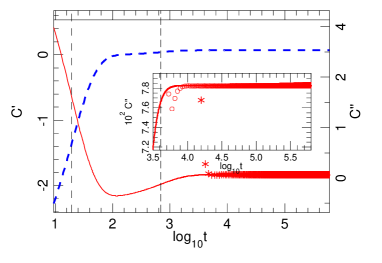
(b)

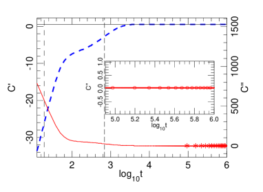
Figure 8: Dynamic heat capacity $C^{\prime}(\omega)$ (blue dashed line, left scale) and $C^{\prime\prime}(\omega)$ (red full line, right scale) of the three-state system, versus time after a temperature jump from $T=0.3$ to $T_{0}=0.08$. The horizontal full line shows the value of the equilibrium heat capacity $C^{\mathrm{eq}}(T_{0})$ on the scale of $C^{\prime}(\omega)$. The dashed vertical lines show the values of $\tau_{1}$ (long dash) and $\tau_{2}$ (short dash). The stars (circles in insets) show the value of $C^{\prime\prime}$ deduced from the entropy production according to GARDEN-RICHARD for $t>2\pi/\omega$ ( condition imposed by the integration over a cycle of the modulation to compute $C^{\prime\prime}$). (a) results for $\omega=10^{-2}$t.u.^-1, (b) results for $\omega=10^{-4}$t.u.^-1.

The first important point to notice is that the dynamic heat capacity, which corresponds to the response of the system at a particular frequency (determined for instance by Fourier transform in the analysis of experimental data) actually shows the strong relaxation phenomena that follow the heat jump, even if their time scale does not match the period of the modulation. This looks surprising at first examination, but this should actually be expected because the relaxations correspond to evolutions within the sample, which modify its thermal response. The physical mechanism of this phenomenon, which may lead to a large time-dependence of the dynamic heat capacity in a strongly out-of-equilibrium system, is the following. Because the rates of the thermally activated transitions $W_{i\to j}$ given by Eq. (5) depend on temperature, they are modulated by the signal $T_{\mathrm{ac}}(t)$. In a first order expansion they include a contribution proportional to $T_{\mathrm{ac}}(t)$. The master equations giving $dP_{i}/dt$ contain products of $P_{j}$ by $W_{i\to j}$, and therefore $dP_{i}/dt$ contains terms proportional to $P_{j}\times T_{\mathrm{ac}}(t)$. They show up in the term $C_{4}$ of Eq. (A) of Appendix A. This coupling of the temperature oscillations with the departure of the probabilities from equilibrium, which follows a temperature jump or a very fast cooling, gives rise to a strong time-dependence of the dynamic heat capacity. Therefore it should be expected that $C^{\prime}(\omega)$, $C^{\prime\prime}(\omega)$, which measure the response of the system to the temperature modulation $T_{\mathrm{ac}}(t)$, follow the relaxation of the system after a large temperature jump, or a very fast cooling. The calculation presented in Appendix A gives a quantitative evaluation of this effect which can cause a strong time-dependence of the dynamic heat capacity. Linear response theory NIELSEN , which treats systems near equilibrium, neglect this coupling and therefore finds that the dynamic specific heat depends on the frequency only, and not on time.

Such large variations of the dynamic heat capacity versus time appear in Fig. 8, which shows that, in the early stage of the evolution, $C^{\prime}(\omega)$ can even be negative. Negative heat capacities have been measured in temperature scans for glasses strongly out of equilibrium THOMAS1931 . Temperature Modulated calorimetry can detect a similar phenomenon during aging at constant temperature after a large temperature jump. Moreover, for dynamic heat capacity, negative values are not surprising, even close to equilibrium, because the theoretical analysis shows that the dynamic heat capacity does not share with the equilibrium heat capacity the property of being always positive FIORE .

(a)

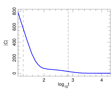
(b)

Figure 9: a) Modulus of the dynamic heat capacity versus time (logarithmic scale) for the three-state system aging after a temperature jump from $T=0.3$ to $T_{0}=0.08$ determined with a temperature modulation at $\omega=10^{-4}$t.u.^-1 (corresponding to the results shown in Fig. 8-b). The dashed vertical lines show the values of $\tau_{1}$ and $\tau_{2}$ at temperature $T_{0}$. b) Experimental result for the aging of a PVAC sample at $24^{\circ}$C after cooling from $90^{\circ}$C at $-1.2^{\circ}$C/min. The modulus of the heat capacity $C_{p}$ was measured at constant temperature using a temperature modulation at $0.1954\,$Hz. (Data from LAARRAJ ).

As shown in Fig. 9-a, when the three-state system ages after a sharp cooling, the modulus of its dynamic heat capacity at fixed frequency may show a large variation with time. This phenomenon takes place although nothing has been modified in the model itself or its parameters. It is due to the large relaxation phenomena following a heat jump discussed above. Actual measurements on aging glasses have also detected strong time dependencies of the modulus of the dynamic heat capacity $|C_{p}|$ at fixed frequency during aging. Figure 9-b shows experimental data for PVAC after a fast cooling LAARRAJ . In a real system, like PVAC, the phenomena are more complex than for the theoretical three-state system, and this simple model would not be sufficient to fit the actual data, but it suggests nevertheless a pathway to understand the experiments. The results for the three-state system clearly show two stages in the aging, associated to the two relaxation times $\tau_{1}$ and $\tau_{2}$. PVAC has a richer spectrum of relaxation times and one cannot readily identify them from the experimental curve of Fig. 9-b. Nevertheless the results suggest at least a very fast relaxation of the order of a few minutes, a second range of relaxation times around 30 minutes, and the presence of longer relaxation times, extending beyond hundreds of minutes as the relaxation is not over at the end of the 1000-minute experiment. The decay with time of the dynamic heat capacity has also been observed by temperature modulated calorimetry for another glassy sample, triphenylolmethane triglycidyl ether TOMBARI2002 . In the discussion of the results, this study considered various possible explanations, such as an evolution of the relaxation times in the sample or indirect effects of structural relaxation leading to a density increase. The simple three-state model cannot attempt to detect subtle effects which are sample-specific, but it shows however that relaxations, with constant characteristic times, are sufficient to generate such a decay of the heat capacity versus time, possibly allowing a simpler analysis of the observations of Tombari et al. TOMBARI2002 .

A theory of the frequency dependent specific heat has been proposed in NIELSEN . It is based on the fluctuation-dissipation theorem and only applies in the vicinity of equilibrium. Our approach, which solves the equations for the time evolution of the occupation probabilities shows that the response of a system very far from equilibrium to a modulation of its temperature can be more complex and includes a contribution coming from the relaxation of the system towards equilibrium. When the system approaches equilibrium, our results converge to the expression given in NIELSEN , but they are more general. The drawback of our approach is that the dynamic equations are solved in the context of a particular model.

Another general analysis of temperature modulated calorimetry has been proposed in GARDEN-RICHARD . It focuses on the origin of the “loss term” $C^{\prime\prime}(\omega)$ and shows that, in the vicinity of equilibrium, it can be quantitatively related to the entropy production integrated over one cycle of the modulation, $\overline{{\cal A}_{s}}$, by

$$\overline{{\cal A}_{s}}=\pi\left(\frac{A_{T}}{T_{0}}\right)^{2}C^{\prime\prime}\;.$$ (11)

The value of $C^{\prime\prime}$ deduced from Eq. (11) is plotted on Fig. 8 (see insets for a magnified scale). It converges towards $C^{\prime\prime}(\omega)$ for all $\omega$ when aging has been long enough to allow the system to come sufficiently close to equilibrium to ensure the validity of the Eq. (11) GARDEN-RICHARD . The results shown on Fig. 8-b is however trivial because the modulation is so slow ($\omega=10^{-4}\,$t.u.^-1) that it probes quasi-equilibrium properties of the system, when entropy production has vanished as well as $C^{\prime\prime}$. Figure 8-a is more interesting because it shows the quantitative validity of the approach of GARDEN-RICHARD .

Figure 8, which shows the evolution of the dynamic heat capacity for two values of $\omega$, suggests that such measurements could allow a study of the various time scales involved when a system ages. The two characteristic times which control the aging for the three-state system are marked on this figure. As discussed above, the large variations of $C^{\prime}(\omega)$ and $C^{\prime\prime}(\omega)$ provide an indirect view of the relaxations toward equilibrium. The shape of $C^{\prime}(\omega)$ gives a first insight on the relaxations in the system because it exhibits two quasi-linear segments centered around $t=\tau_{1}$ and $t=\tau_{2}$. In a system with a more complex spectrum of aging timescales, performing experiments for different values of $\omega$ may give a quantitative information on this spectrum. The simulation with $\omega=10^{-4}\,$t.u.^-1 probes the evolution of the system up to timescales larger than $\tau_{2}$ and therefore a quasi-equilibrium situation. This is why, in the long term $C^{\prime}(\omega)$ tends to $C^{\mathrm{eq}}(T_{0})$. Conversely for $\omega=10^{-2}\,$t.u.^-1, even in the large time limit $C^{\prime}(\omega)$ stays well below $C^{\mathrm{eq}}(T_{0})$ because the time scale of the modulation does not allow the system to relax the degrees of freedom which evolve with characteristic time $\tau_{2}$. Thus studying

$$\Delta C(\omega)=C^{\mathrm{eq}}(T_{0})-\lim_{t\to\infty}C^{\prime}(\omega,t)$$ (12)

versus $\omega$ provides some measure of the relaxation times that govern aging in the system and of the magnitude of the contribution to the dynamic heat capacity of the degrees of freedom associated to each of these relaxation times.

III.3 Investigating the Kovacs effect by temperature modulated calorimetry

The Kovacs effect is an interesting effect which points out the peculiarities of out-of-equilibrium systems KOVACS . To our knowledge it has not been investigated by temperature modulated calorimetry although such experiments could provide useful insights on its mechanism. It was observed in a series of two experiments. First a glass sample is slowly cooled to record the variation of its volume versus temperature $v^{\mathrm{eq}}(T)$ in quasi-equilibrium. In a second experiment, the sample is abruptly cooled from an initial temperature $T_{1}$ to a low temperature $T_{2}$ in the vicinity of the glass transition temperature $T_{g}$. The sample is let to age at $T_{2}$. Its volume slowly decreases. When the volume has reached the value $v_{0}$ that it would have at equilibrium at some temperature $T_{0}>T_{2}$, $v_{0}=v^{\mathrm{eq}}(T_{0})$, the temperature of the sample is abruptly switched from $T_{2}$ to $T_{0}$. At this point the volume and temperature of the sample are the same as if it was in equilibrium at temperature $T_{0}$. However this state has not be reached by a quasi-equilibrium trajectory. Therefore the sample is not in equilibrium. Kovacs observed that, when it is maintained at $T_{0}$, its volume starts to increase, and then decays until the system slowly reaches equilibrium at $T_{0}$ with volume $v^{\mathrm{eq}}(T_{0})$.

For the three-state system, a volume is not defined, but nevertheless the Kovacs effect can be observed by following the energy versus time PG . Figure 10 shows an example from a numerical simulation. From an equilibrium state at $T_{1}=0.3$, the three-state-system (using the same model parameters as above in Sec. III.1) was abruptly switched to $T_{2}=0.02$ and let to age for $1.8\,10^{7}$t.u. Its energy decreases slowly during this aging at very low temperature, and, at the end of the aging period it has reached $E^{\mathrm{eq}}(T=0.17856)$. Then the system is abruptly switched from $T_{2}=0.02$ to $T_{0}=0.17856$ and we monitor its energy versus time in the presence of a small temperature modulation $T_{\mathrm{ac}}$ with $A_{T}=8\,10^{-4}$ and various values of $\omega$. Figure 10 shows an example for $\omega=10^{-2}\;$t.u.^-1. It exhibits the same “Kovacs hump” as the one observed by Kovacs for the volume of a glass KOVACS . Although, at the beginning of the scan at temperature $T_{0}$ the system has the energy $E^{\mathrm{eq}}(T=0.17856)$, while it ages at $T_{0}$ its energy rises significantly before coming back to its equilibrium value. Figure 10 shows that the maximum occurs at a time which is intermediate between the two relaxation times $\tau_{1}$ and $\tau_{2}$ of the three-state model at temperature $T_{0}$. This suggests that the shape of the Kovacs hump is governed by the relaxation spectrum of the sample. It would be interesting to check this experimentally with a glassy sample. Temperature Modulated calorimetry, which probes this spectrum should be the appropriate technique. To test this idea, we have investigated the evolution versus time of $C^{\prime}(\omega)$ and $C^{\prime\prime}(\omega)$ during a Kovacs scan of the three-state system.

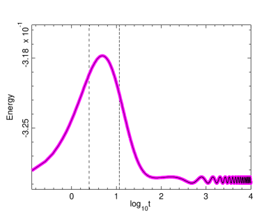
Figure 10: Energy versus time for a Kovacs scan with the three-state system. After a sharp temperature jump from $T_{1}=0.3$ to $T_{2}=0.02$ the model was let to age at $T_{2}$. Its energy decreases and, when it had reached the value $E^{\mathrm{eq}}(T=0.17856)$, the temperature was abruptly switched to $T=T_{0}+T_{\mathrm{ac}}$ with $T_{0}=0.17856$ and $T_{\mathrm{ac}}=A_{T}\sin\omega t$, $A_{T}=8\,10^{-4}$, $\omega=10^{-2}\;$t.u.^-1. The figure shows the energy of the system versus the time (in logarithmic scale) from the temperature jump from $T_{2}$ to $T_{0}$. The thick magenta line shows the energy recorded during the numerical simulation, while the thin black line, along the magenta line, shows the result of the analytical calculation of the energy following the process presented in Appendix A, starting from the initial state reached at the end of the aging period at $T_{2}$. The black vertical dashed lines mark the relaxation times of the three state system at temperature $T_{0}$.

Figure 11 shows the result for two values of $\omega$. As shown in Fig. 10, the analytical calculation of the energy versus time, as discussed in Appendix A, matches the variation recorded in the numerical simulation. This allows us to use the heat capacity calculated analytically, which is more accurate than relying on a numerical treatment of the simulation results, especially for a case where the heat capacity depends on time.

(a)

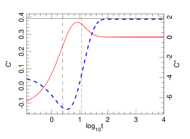
(b)

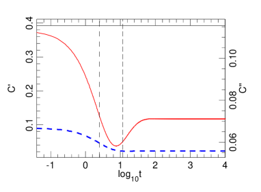
Figure 11: Dynamic heat capacity $C^{\prime}(\omega)$ (blue dashed line, left scale) and $C^{\prime\prime}(\omega)$ (red full line, right scale) of the three-state system, versus time during the Kovacs scan shown in Fig. 10. The horizontal black line shows the value of the equilibrium heat capacity $C^{\mathrm{eq}}(T_{0})$ on the scale of $C^{\prime}(\omega)$. The dashed vertical lines show the values of $\tau_{1}$ and $\tau_{2}$. (a) results for $\omega=10^{-2}\,$t.u.^-1, (b) results for $\omega=1\,$t.u.^-1.

Figure 11 shows that both $C^{\prime}$ and $C^{\prime\prime}$ vary significantly with time. This is not surprising because we have shown in Sec. III.2 that, although temperature modulated calorimetry records the value of the heat capacity at a specific frequency, the values of $C^{\prime}(\omega)$ and $C^{\prime\prime}(\omega)$ also reflect the relaxations which occur within the sample. However the recorded signal is filtered in frequency because it is detected through the response to an oscillatory driving. This is what makes temperature modulated calorimetry particularly attractive to study the Kovacs effect. On one hand it does reflect the evolutions which occur within the sample while it ages during the Kovacs scan, as attested by the large variations of $C^{\prime}$ and $C^{\prime\prime}$ which take place in the same time scale as the variation of the energy of Fig. 10. But, on the other hand, the variation of $C^{\prime}(\omega)$ and $C^{\prime\prime}(\omega)$ give a quantitative picture of the time scales at which the sample evolves. The relaxation frequencies for the model at temperature $T_{0}$ are $\omega_{1}=2\pi/\tau_{1}=2.5427\;$t.u.^-1 and $\omega_{2}=2\pi/\tau_{2}=0.54193\;$t.u.^-1. Figure 11-a shows the dynamic heat capacity measured with a frequency $\omega=10^{-2}\;$t.u.^-1, which probes the dynamic of the system at times scales longer than its internal time scales. This is clear from the results because the value of $C^{\prime}(\omega)$ which starts with a value well below the equilibrium specific heat of the sample at $T_{0}$, $C^{\mathrm{eq}}(T_{0})$, and even temporary drops below $0$, finally reaches $C^{\mathrm{eq}}(T_{0})$ in the long term, which indicates that the system had time to reach a quasi-equilibrium on the time scale which is probed. Figure 11-b shows the heat capacity measured with a frequency $\omega^{\prime}=1\;$t.u.^-1, $\omega_{2}<\omega^{\prime}<\omega_{1}$, which probes timescales larger than $\tau_{1}$ but only those smaller than $\tau_{2}$. As a result $C^{\prime}(\omega^{\prime})$ exhibits a significant time-dependence, which indicates that the evolution within the sample contains some degrees of freedom which evolve faster than $2\pi/\omega^{\prime}$. However, in the long term $C^{\prime}(\omega^{\prime})$ does not reach $C^{\mathrm{eq}}(T_{0})$. This indicates that there are other degrees of freedom which are slower than $2\pi/\omega^{\prime}$. Another simulation with $\omega^{\prime\prime}=4\;$t.u.^-1, i.e. $\omega^{\prime\prime}>\omega_{1}>\omega_{2}$ finds that both $C^{\prime}(\omega^{\prime\prime})$ and $C^{\prime\prime}(\omega^{\prime\prime})$ stay very small during the whole simulation, indicating that all degrees of freedom are slower than $2\pi/\omega^{\prime\prime}$. These results show how a study of the dynamic heat capacity versus $\omega$ for an experimental Kovacs scan might clarify the role of the thermal relaxation spectrum in the shape of the Kovacs hump of a glass.

IV Scanning Calorimetry versus Temperature Modulated Scanning Calorimetry

IV.1 Experimental results

Figure 12 points out a qualitative difference between Differential Scanning Calorimetry (DSC) measurements and $C^{\prime}(\omega)$ determined by a Modulated Temperature Scanning Calorimetry (MTSC) experiment for a PVAC sample which had been preliminary quickly cooled from a temperature above its glass transition temperature. The MTSC results show a rise of the specific heat which becomes smoother when the frequency of the temperature modulation increases. This is expected and it is consistent with our discussions of Sec. III. A calorimetry experiment with temperature modulated at frequency $\omega$ is only sensitive to degrees of freedom which are faster that $2\pi/\omega$. For a system like PVAC, which has a continuous spectrum of relaxation times, the variation of $\omega$ does not detect qualitative changes when $\omega$ crosses specific relaxation frequencies but instead a smoother change. This nevertheless shows that, when the frequency of modulation increases, the number of channels which contribute to the energy exchange at a given temperature decreases. As a result higher temperatures are necessary to approach the equilibrium specific heat.

Although the DSC and MTSC experiments have used the same heating rate for the temperature ramp, the DSC curve shows a hump which is not observed in the MTSC measurements. One may ask weather this is only a matter of time scales so that lower and lower values of $\omega$ could finally probe the hump observed in DSC, or if there is a fundamental reason that prevents MTSC from detecting some of the phenomena that DSC probes. This is an important question for calorimetry methodology. Using a test “sample” such as the three-state system allows us to give an unambiguous answer, as shown in the next section.

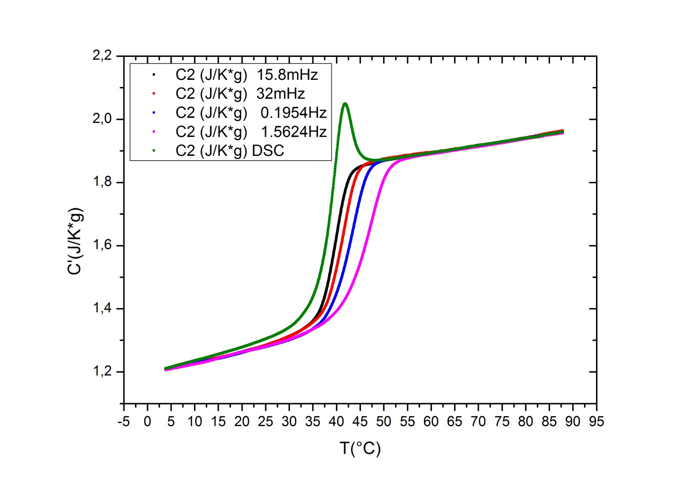
Figure 12: Comparison between scanning calorimetry results and temperature modulated calorimetry experiments for a PVAC sample after fast cooling (Data from LAARRAJ ). The sample was cooled from $90^{\circ}$C down to $4^{\circ}$C, with a cooling rate of $-1.2^{\circ}$C/minute. The green curve, with a maximum around $T=40^{\circ}$C, shows the result of a standard Differential Scanning Calorimetry (DSC) experiment during which the sample is heated at the rate of $+1.2^{\circ}$C/minute. The other curves show $C^{\prime}(\omega)$ determined from temperature modulated scanning calorimetry (MTSC), with a temperature $T(t)=T_{0}(t)+T_{\mathrm{ac}}(t)$. $T_{0}(t)$ is a temperature ramp with heating rate $+1.2^{\circ}$C/minute, and the frequency of the modulated part, $\nu=\omega/2\pi$, has the values $15.8\,10^{-3}$Hz (for the curve with the steepest rise), $32\,10^{-3}$Hz, $0.1954\,$Hz and $1.5624\,$Hz for the curve with the slowest rise.

IV.2 Analysis with a model system

As shown in the previous sections, the three state system can be used as a sample system to bring further insights on the methods of calorimetry because it allows a detailed analysis of the phenomena which is not possible from experiments alone. The equivalent of a DSC experiment is obtained by imposing a temperature ramp $T_{1}(t)=T_{0}\pm st$ where $s$ is a slope which measures the variation of temperature per time unit and the $\pm$ sign allows for heating or cooling. In a simulation we can record the energy $E(t)$ of the system and compute its heat capacity $C_{DSC}=dE/dT$.

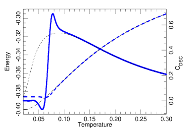
Figure 13: Results of the simulation of a DSC experiment with the three-state system. The thick dashed blue line shows the energy (left scale) versus temperature during a heating ramp from $T=0.02$ to $T=0.3$ in $10^{5}$t.u. after cooling from equilibrium at $T=0.3$ down to $T=0.02$ in the same time interval. The thin black dashed line shows the equilibrium energy $E^{\mathrm{eq}}(T)$ (Eq. (3) ). The thick full blue line shows $C_{DSC}(T)=dE/dT$ (right scale) during this heating scan and the thin black dotted line shows the equilibrium specific heat $C^{\mathrm{eq}}(T)$ (Eq. (4) ).

Figure 13 shows the result of such a numerical experiment. The three-state system, with the same parameters as above, was first cooled from an equilibrium state at $T=0.3$ down to $T=0.02$ in $10^{5}\,$t.u. . In the first stage of the cooling its energy $E_{DSC}(t)$ followed the curve $E^{\mathrm{eq}}(T)$ but below $T\approx 0.08$ it decreased slower and, at the end of the cooling scan the system was out of equilibrium. Figure 13 shows the data for the heating process from $T=0.02$ to $T=0.3$, which followed the cooling, with a linear heating ramp in $10^{5}\,$t.u. . Below $T\approx 0.13$, the heat capacity $C_{DSC}(T)$ shows strong deviations from the equilibrium heat capacity $C^{\mathrm{eq}}(T)$. The sharp rise when temperature rises above $T\approx 0.07$, followed by a hump, occurs at the temperature at which the relaxation times of the system have sufficiently decreased to allow transitions between states during the characteristic time of the heating ramp. This is typical for a DSC scan with a sample initially out of equilibrium, and displays qualitative similarities with the hump observed experimentally with PVAC (Fig. 12).

The analogous of a MTSC experiment is obtained by adding a small temperature modulation to the heating ramp

$$T(t)=T_{1}(t)+T_{\mathrm{ac}}(t)=T_{0}+s\,t+A_{T}\,\sin\omega t\;.$$ (13)

As a result, in addition to the increase of the energy due to the heating ramp, the energy has an additional oscillatory component $E_{\mathrm{ac}}(t)$. In an experiment this modulated part is usually extracted by Fourier transform. In our simulations, it can be obtained by subtracting $E_{DSC}(t)$ from the value $E_{MTSC}(t)$ recorded during the simulation with the additional modulation $T_{\mathrm{ac}}(t)$.

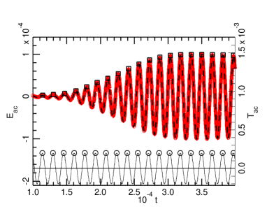
Figure 14: $E_{\mathrm{ac}}(t)$, (thick red line, left scale) the fraction of the energy which is modulated due to the modulated temperature $T_{\mathrm{ac}}$ in a simulation of an MTSC experiment ($\omega=4\;10^{-3}\,$t.u.^-1). This figure only plots a fraction of the heating scan, which lasts from $t=0$ to $t=0.4\;10^{5}\,$t.u. in order to show the details of the modulation. The sinusoidal black line at the bottom shows $T_{\mathrm{ac}}(t)$ (right scale). The squares and circles mark the maxima of $E_{\mathrm{ac}}(t)$ and $T_{\mathrm{ac}}(t)$ which are used to calculate the modulus and phase of the specific heat as explained in the text. The dashed black line along the thick red line for $E_{\mathrm{ac}}(t)$ is an analytical result for $E_{\mathrm{ac}}(t)$ discussed in the text.

Figure 14 shows $E_{\mathrm{ac}}(t)$ for a portion of the heating scan with $A_{T}=2\,10^{-4}$ and $\omega=4\,10^{-3}\,$t.u.^-1 (corresponding to a period of $\tau_{\omega}=1571\,$t.u.). The numerical results can be used to calculate the magnitude $C(\omega)$ of the frequency-dependent heat capacity and its phase $\Phi$, using an approach which mimics the experimental approach. We look for the values and dates of the maxima $E_{\mathrm{ac}}^{\mathrm{max}}(t_{j})$ of $E_{\mathrm{ac}}(t)$ and $T_{\mathrm{ac}}^{\mathrm{max}}(t_{k})$ of $T_{\mathrm{ac}}(t)$. Then for each maximum $k$ of $T_{\mathrm{ac}}(t)$, we look for the closest maximum $j$ of $E_{\mathrm{ac}}(t)$ and we define

$$C(\omega,t_{k}) =E_{\mathrm{ac}}^{\mathrm{max}}(t_{j})/T_{\mathrm{ac}}^{\mathrm{max}}(t_{k})$$

$$\Phi(t_{k}) =2\pi(t_{j}-t_{k})/\tau_{\omega}$$

The values of $C(\omega)$ and $\Phi(t_{k})$ are obtained at time $t_{k}$, when the temperature of the sample can be considered to be $T_{1}(t_{k})$ because $T_{\mathrm{ac}}\ll T_{1}$.

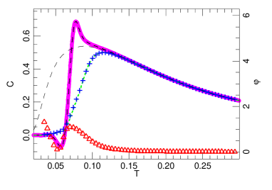
Figure 15: Heat capacity in a simulated MTSC experiment ($\omega=4\;10^{-3}\,$t.u.^-1). The blue crosses show the magnitude of $C(\omega)$, determined with Eq. (IV.2) from the maxima of $E_{\mathrm{ac}}$ and $T_{\mathrm{ac}}$, versus the temperature $T_{1}(t)$ of the heating ramp. The red triangles show its phase $\Phi$ with respect to the temperature modulation. The figure also shows $C_{DSC}(T)$ for the same sample system (thick magenta curve) and the equilibrium heat capacity (thin black dashed line). The dash black line which follows $C_{DSC}(T)$ and the dotted green line along the $C(\omega)$ crosses are analytical results discussed in the text.

Figure 15 shows the modulus of the dynamic heat capacity versus the temperature $T_{1}(t)$ of the heating ramp, and its phase relative to the temperature modulation. The equilibrium specific heat $C^{\mathrm{eq}}(T)$ and $C_{DSC}(T)$ are also plotted for comparison. At low temperature $C(\omega)$ deviates significantly from $C^{\mathrm{eq}}(T)$, which is expected because, in this temperature range, thermal relaxation is very slow. The relaxation times $\tau_{1}$ and $\tau_{2}$ for the two eigenmodes are well above the period of the temperature modulation as shown in Fig. 4 so that the response of the system to the modulation is weak. When temperature increases, $\tau_{1}$ and $\tau_{2}$ decrease and $C(\omega)$ tends to $C^{\mathrm{eq}}(T)$. For the same reason the phase shift $\Phi$ is large at low temperature and tends to $0$ when $C(\omega)$ approaches $C^{\mathrm{eq}}(T)$. Around $T=0.05$ the phase shift shows an oscillation which could be related to contribution of the metastable states getting destabilized by the temperature rise, but this is not reflected by any hump in $C(\omega)$ which shows a monotonous rises towards $C^{\mathrm{eq}}(T)$, as observed experimentally for PVAC (Fig. 12).

Figure 16 shows how these results depend on the frequency $\omega$ of the modulation. When $\omega$ increases (Fig. 16-a) the experiment probes faster and faster time scales. Higher temperatures are needed to bring the relaxation times of the system in the range of the time scales which are detected, so that $C(\omega)$ grows more slowly with $T$ and only approaches $C^{\mathrm{eq}}(T)$ at higher temperatures. Conversely, for very slow modulations (Fig. 16-b), the maximum slope of $T_{\mathrm{ac}}(t)$ decreases so much that it is no longer much greater than the slope of the heating ramp. In this case the rise of $C(\omega)$ versus $T$ becomes as fast as the rise of $C_{DSC}(T)$ in the range $T\approx 0.05-0.08$. Nevertheless, in agreement with the experimental observations (Fig. 12) the simulation does not show any anomaly such as the hump in specific heat observed in scanning calorimetry. This suggests that there is a fundamental difference between the results which can be obtained by DSC and by MTSC.

(a)

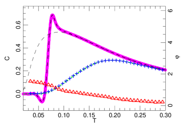
(b)

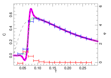
Figure 16: Same as Fig. 15 for two other values of the frequency of the temperature modulation: a) $\omega=0.1\,$t.u.^-1 and b) $\omega=10^{-3}\,$t.u.^-1. For this very slow modulation, the period $\tau_{\omega}=0.63\,10^{4}\,$t.u. becomes significant with respect to the duration of the heating ramp $10^{5}\,$t.u. and we have indicated the time interval between two maxima by horizontal error bars.

However numerical experiments, like actual experiments, provide observations but they do not give a full picture of the mechanisms which act behind the scene to lead to these observations. Fortunately, working with a tractable model system allows us to go beyond observations because analytical calculations are possible to analyze the data and they are revealing.

In Sec. III and appendix A we showed that the time evolution of the energy of the three-state system at temperature $T(t)=T_{0}+T_{\mathrm{ac}}(t)$ can be calculated analytically when $T_{0}$ is a constant. The method can be extended if $T_{0}$ is replaced by a temperature ramp $T_{1}(t)$, although the solution cannot be expressed in closed form, by dividing the ramp in small time intervals $\Delta t=[t_{j},t_{j+1}]$. In such an interval $T_{0}$ is replaced by $T_{1}(t_{j})$ which can be treated as constant if $\Delta t$ is sufficiently small with respect to the relaxation times $\tau_{1}[T_{1}(t_{j})]$, $\tau_{2}[T_{1}(t_{j})]$. Knowing the occupation probabilities $P_{1}(t_{j})$, $P_{2}(t_{j})$, the calculation presented in Appendix A allows us to calculate $P_{1}(t_{j+1})$, $P_{2}(t_{j+1})$ in the presence of the temperature modulation. This defines the initial state for the next time interval so that we can proceed step by step from the start to the end of the temperature ramp. As the calculation proceeds the eigenmodes and relaxation times $\tau_{1}$, $\tau_{2}$ have to be recalculated according to the change of $T_{1}(t)$ from one interval to the next. However, as this calculation is fast, we can select a very small value for $\Delta t$ to ensure a good accuracy to the process which would converge to an exact result in the limit $\Delta t\to 0$. In practice we used $\tau_{\omega}/5000\leq\Delta t\leq\tau_{\omega}/500$.

The interest of this calculation is not to make sure that the analytical calculation can reproduce the simulation results (which it does) but to understand the origin of the observations. We showed that the analytical calculation proceeds by expressing the occupation probabilities as

$$P_{i}(t)=P_{i}(T_{\mathrm{ref}})+\widetilde{Q_{i}}(t)+q_{i}(t)$$ (15)

$T_{\mathrm{ref}}$ being either $T_{0}$ or $T_{1}(t_{j})$. $\widetilde{Q_{i}}(t)$ is the solution that we would get in the absence of modulation and $q_{i}(t)$ is an additional contribution which is entirely due to the modulation. As shown by Eq. (A) the energy splits into

$$E(t)=\widetilde{E}(t)+e(t)\;$$ (16)

where $\widetilde{E}(t)$ depends on $\widetilde{Q_{i}}(t)$ and $e(t)$ depends on $q_{i}(t)$. This expression can therefore be directly related to the experimental results. A temperature ramp without modulation corresponds to a DSC experiment. Therefore $\widetilde{E}(t)$ should correspond to the energy measured by DSC and $d\widetilde{E}(t)/dT_{1}(t)$ should give $C_{DSC}(T)$. Figures 15 and 16 show that this is exactly the case: the dashed black line which follows the magenta line deduced from the numerical simulation of a DSC experiment (Fig. 13) plots $d\widetilde{E}(t)/dT_{1}(t)$. Equation (16) also tells us that $e(t)=E(t)-\widetilde{E}(t)$ is the contribution of the modulation to the energy, i.e. $E_{\mathrm{ac}}(t)$ in an experiment. Again we can verify this to a good accuracy on Fig. 14 as the dashed black line which follows the thick red line plotting $E_{\mathrm{ac}}(t)$ in a simulated MTSC experiment is the curve for $e(t)$ deduced from the analytical calculation. Therefore the analytical derivative of $e(t)$ gives the dynamic heat capacity of the system. We calculate the time derivative $de(t)/dt$ and extract from this expression the prefactor of $\sin\omega t$ (in phase with $T_{\mathrm{ac}}(t)$) and the prefactor of $\cos\omega t$ (in quadrature of phase with $T_{\mathrm{ac}}(t)$). Dividing these two prefactors by the amplitude of $dT_{\mathrm{ac}}(t)/dt=A_{T}\omega$ we get $C^{\prime}(\omega)$ and $C^{\prime\prime}(\omega)$. Then the modulus of the dynamic heat capacity is readily obtained as $C(\omega)=\big{[}C^{\prime}(\omega)^{2}+C^{\prime\prime}(\omega)^{2}\big{]}^{1/2}$. The green lines on Figs. 15 and 16 show that the analytical expression of $C(\omega)$ exactly follows the simulation results.

These results demonstrate that, for a glassy system out of equilibrium, $C_{DSC}$ and $C(\omega)$ are fundamentally different quantities. $C_{DSC}$ measures the relaxations due to the temperature drift, i.e. the response to $T_{1}(t)$, while $C(\omega)$ only selects the oscillatory response to $T_{\mathrm{ac}}(t)$. Therefore we should not expect that $C(\omega)$ should converge to $C_{DSC}$ in the limit $\omega\to 0$. This explains why experimental measurements of these two quantities differ as shown in Sec. IV.1. $C(\omega)$ do captures some components of $C_{DSC}$ because the slope of its rise when $T$ increases grows and tends towards the slope of the rise of $C_{DSC}(T)$, but $C(\omega)$ misses the extra humps which are pure relaxation phenomena. Actually, as shown in Sec. III, relaxations are not entirely absent from the dynamic heat capacity because they enter in a correction factor for the amplitude of the response to $T_{\mathrm{ac}}(t)$ (see Eqs. (64) and (A) ). Those corrections could play a significant role for the temperature jumps discussed in Sec. III, but they become negligible when temperature varies continuously. They might become noticeable if the variation $T_{1}(t)$ could become very fast. But this cannot be the case in an scanning experiment which intends to measure the response to an oscillatory temperature component. Experimentally the oscillation can only be detected if the maximum slope of $T_{\mathrm{ac}}(t)$ is larger than the slope of $T_{1}(t)$. For $\omega=10^{-3}\,$t.u.^-1 Fig. 16 shows that, even in this extreme case with only about 16 periods of $T_{\mathrm{ac}}(t)$ during the full heating ramp, the relaxation humps observed in $C_{DSC}(T)$ do not show up in $C(\omega,T)$.

V Discussion

In this paper we have used a combination of numerical simulations and analytical calculations for a model system, as well as comparisons with actual experimental data for a glassy system, to provide a deeper understanding of temperature modulated calorimetry measurements which have been at the origin of many discussions GARDEN-REVIEW . We have essentially considered two questions:

• how does the signal looks when one performs experiments with a small temperature modulation added to a constant underlying temperature ? In particular we examined how the dynamic heat capacity may depend on time in this case.

• for scanning calorimetry with an underlying temperature which varies as a ramp, is there a fundamental difference between a standard calorimetry method such as DSC and a temperature modulated calorimetry measurement such as MTSC ?

In the case of a constant underlying temperature we showed that, as expected, temperature modulated calorimetry probes the spectrum of the relaxation times of the sample system. The energy oscillates with some phase shift with respect to the temperature modulation and these oscillations are accompanied by an entropy production which varies at twice the frequency of the temperature modulation because entropy is created when temperature moves up and down.

As a sample system we investigated the three-state system which is the simplest system with a non-trivial, non-single-frequency spectrum of the fluctuations of the energy transfers PG . This simple system allows a full analytical calculation of the dynamic specific heat which has a component in phase with the temperature modulation but also a component in quadrature with it. These two contributions are often designated as a “complex” heat capacity. Using a complex notation to compute $C(\omega)$ is however misleading because it focuses on a steady response, and does not explicitly introduces the boundary conditions in the solution. Those boundary conditions may be important because temperature modulated calorimetry measurements probe not only the spectrum of the energy transfers in the sample but also the time evolution of the state of the system, such as its aging. After a sharp temperature jump the system may undergo strong relaxations, and we showed that these relaxations appear even in the oscillatory component of the energy. In measurements they show up as a time-dependent heat capacity. A spectacular example is provided by the Kovacs effect for glasses. To our knowledge it has never been investigated by temperature modulated calorimetry, although our study shows how such measurements could clarify its origin because the duration of the Kovacs hump is related to the time scales which govern the internal evolution of the glass.

In the case of scanning calorimetry experiments for out-of-equilibrium glassy systems, we showed that standard experiments such as DSC and measurements with an oscillatory temperature such as MTSC probe intrinsically different properties of the system. The analytical calculation explains why, even in the limit of very low modulation frequency, some of the features observed in DSC do not show up in MTSC. Besides the case of PVAC presented in Fig. 12 and in ref. LAARRAJ , the differences between DSC and MTSC experimental results have been discussed in various papers ANDROSCH ; SARUYAMA ; GARDEN2004 ; GARDEN2005 . All studies confirm that, at high modulation frequency, the MTSC measurements detect a lower value of the heat capacity than DSC because they are only sensitive to energy transfers which are fast enough to take place within one period of the modulation. However these studies show that it is important to distinguish between experiments that study thermodynamic transitions, for instance in paraffin SARUYAMA or PTFE ANDROSCH ; GARDEN2005 , and protein folding GARDEN2004 , which could be observed at equilibrium or quasi-equilibrium in very slow temperature scans, from observations of out-of-equilibrium effects in glasses LAARRAJ . For equilibrium transitions, near the transition temperature, in the limit $\omega\to 0$ the modulation of the temperature is sufficient to change the fraction of the sample which has passed the transition. Therefore, in this case integrating $C(\omega,T)$ versus $T$ around the transition temperature and taking the limit $\omega\to 0$ recovers the value of the latent heat GARDEN2005 . Conversely, experiments with glasses out of equilibrium, and calculations for the three-state model, show that the relaxations detected by $C_{DSC}$ are different from the dynamic heat capacity measured by ac-calorimetry, even in the limit $\omega\to 0$. This is because the evolution of the system is not caused by the temperature modulation. Instead the strongly out-of-equilibrium initial state tends to spontaneously evolve towards equilibrium when $T$ is raised in the DSC scan.

Although the conclusions based on the analytical calculations have been obtained with a particular model, the three-state system, we think that they have a much broader validity because this model is very generic. It describes a sample with a free energy landscape which has many metastable minima, and which evolves between them under the effect of thermal fluctuations. These are features which have been proposed for glasses and complex liquids STILLINGER-82 as well as proteins NAKAGAWA , but can be expected to apply to many systems. Numerical simulations of a bead-spring polymer model known to be a glass-former have shown that, at low temperature, the low frequency component of $C^{\prime\prime}(\omega)$ is entirely the result of the dynamics of the system within its inherent structures, i.e. the minima of its potential energy landscape BROWN-JR2011 . With only two relaxation times, the three-state system is the simplest example of a large family which has a non-trivial spectrum. It is sufficient to test some ideas on temperature modulated calorimetry, for instance by showing how a scan in the modulation frequency $\omega$ detects one frequency after another. For a real system with many relaxation times, the analytical calculations that we developed in the appendices cannot be carried out in practice, but the methods are, in principle, still valid, at the expense of large matrices of eigenstates. Therefore, the qualitative aspects of our results should be preserved, such as for instance the fundamental difference between DSC and MTSC results for a glass. This assumption is supported by the results on PVAC that we presented. And actually, as shown in PG the three-state system itself could be of interest to analyze various experimental observations, in cases where the simple two-state system, with a single relaxation, fails. This model only describes the configurational heat capacity. This is indeed a limitation but, in many systems it is however the contribution which is the most interesting because vibrational or electronic contributions are generally smoother versus temperature or significantly weaker TOMBARI2007 .

Appendix A Analytical calculation of the energy of the three-state system at modulated temperature.

We consider the case of a temperature modulation around a fixed average value $T_{0}$, $T(t)=T_{0}+T_{\mathrm{ac}}(t)=T_{0}+A_{T}\sin\omega t$. To get the energy $E(t)=\sum_{i=1}^{3}P_{i}(t)E_{i}$, given an initial state of the system at time $t=0$ determined by $P_{i}(t=0)$, we must solve the set of equations (II) and the similar equations for $P_{2}$ and $P_{3}$, with $\omega_{ij}=1$ and the condition $\sum_{i=1}^{3}P_{i}=1$.

It is convenient to introduce the variables $Q_{i}(t)=P_{i}(t)-P_{i}^{\mathrm{eq}}(T_{0})$ where $P_{i}^{\mathrm{eq}}(T_{0})$, henceforth denoted by $P_{i}^{0}$, are the equilibrium probabilities at temperature $T_{0}$. The condition $\sum_{i=1}^{3}P_{i}=1$ implies $\sum_{i=1}^{3}Q_{i}=0$, so that $E(t)$ is determined by $Q_{1}$ and $Q_{2}$ only. Note that we make no assumption regarding the size of $Q_{i}$ compared to $P_{i}^{\mathrm{eq}}$. In strongly out-of-equilibrium situations it may happen that $|Q_{i}/P_{i}^{\mathrm{eq}}|\gg 1$.

As we assume $T_{\mathrm{ac}}\ll T_{0}$, the rates of the thermally activated transitions $W_{ij}(t)$ (Eq. 5) can be expanded around their values $W_{ij}^{0}$ at temperature $T_{0}$ to first order in $T_{\mathrm{ac}}$ as

$$W_{ij}(t)=W_{ij}^{0}+T_{\mathrm{ac}}(t)\frac{B_{ij}}{T_{0}^{2}}W_{ij}^{0}\;.$$ (17)

Using these expansions, the equation for $dQ_{1}/dt$, deduced from Eq. (II) splits into 4 components

$$\frac{dQ_{1}}{dt}=C_{1}+C_{2}+C_{3}+C_{4}\;,$$ (18)

with

$$C_{1} =-P_{1}^{0}W_{12}^{0}+P_{2}^{0}W_{21}^{0}-P_{1}^{0}W_{13}^{0}+P_{3}^{0}W_{31}^{0}$$

$$C_{2} =-Q_{1}\left[W_{12}^{0}+W_{13}^{0}+W_{31}^{0}\right]+Q_{2}\left[W_{21}^{0}-W_{31}^{0}\right]$$

$$C_{3} =T_{\mathrm{ac}}\frac{1}{T_{0}^{2}}\left[-P_{1}^{0}B_{12}W_{12}^{0}-P_{1}^{0}B_{13}W_{13}^{0}\right.$$

$$\qquad\qquad\left.+P_{2}^{0}B_{21}W_{21}^{0}+P_{3}^{0}B_{31}W_{31}^{0}\right]$$

$$C_{4} =-Q_{1}\frac{T_{\mathrm{ac}}}{T_{0}^{2}}\left[B_{12}W_{12}^{0}+B_{13}W_{13}^{0}+B_{31}W_{31}^{0}\right]$$

$$~{}\qquad+Q_{2}\frac{T_{\mathrm{ac}}}{T_{0}^{2}}\left[B_{21}W_{21}^{0}-B_{31}W_{31}^{0}\right]$$

$$\;.$$ (19)

Component $C_{1}$ vanishes due to the detailed balance condition at temperature $T_{0}$. Component $C_{2}$, in which we used $Q_{3}=-(Q_{1}+Q_{2})$, is of the form $C_{2}=-AQ_{1}+BQ_{2}$ if we introduce the notations $A$ and $B$ of the two brackets that it contains. Component $C_{3}$ can be written $C_{3}=T_{\mathrm{ac}}\gamma_{1}$ by introducing a notation for the bracket divided by $T_{0}^{2}$ and component $C_{4}$ can be written $C_{4}=-CQ_{1}T_{\mathrm{ac}}+DQ_{2}T_{\mathrm{ac}}$ by introducing $C$ and $D$ to designates the two brackets divided by $T_{0}^{2}$. The quantities $A$, $B$, $C$, $D$ and $\gamma_{1}$ are time independent, while $T_{\mathrm{ac}}=A_{T}\sin\omega t$ depends on time. A similar calculation for the time evolution of $Q_{2}$ leads to

$$\frac{dQ_{2}}{dt}=B^{\prime}Q_{1}-A^{\prime}Q_{2}+T_{\mathrm{ac}}\gamma_{2}+D^{\prime}Q_{1}T_{\mathrm{ac}}-C^{\prime}Q_{2}T_{\mathrm{ac}}$$ (20)

with

$$A^{\prime} =W_{21}^{0}+W_{23}^{0}+W_{32}^{0}$$

$$B^{\prime} =W_{12}^{0}-W_{32}^{0}$$

$$\gamma_{2} =\frac{1}{T_{0}^{2}}\left[-P_{2}^{0}B_{21}W_{21}^{0}-P_{2}^{0}B_{23}W_{23}^{0}\right.$$

$$\qquad\qquad\left.+P_{1}^{0}B_{12}W_{12}^{0}+P_{3}^{0}B_{32}W_{32}^{0}\right]$$

$$C^{\prime} =\frac{1}{T_{0}^{2}}\left[B_{21}W_{21}^{0}+B_{23}W_{23}^{0}+B_{32}W_{32}^{0}\right]$$

$$D^{\prime} =\frac{1}{T_{0}^{2}}\left[B_{12}W_{12}^{0}-B_{32}W_{32}^{0}\right]$$

The equations for $Q_{1}$ and $Q_{2}$ can therefore be put in the matrix form

$$\frac{d}{dt}\left(\begin{array}[]{c}Q_{1}\\ Q_{2}\end{array}\right) =\left(\begin{array}[]{cc}-A&B\\ B^{\prime}&-A^{\prime}\end{array}\right)\left(\begin{array}[]{c}Q_{1}\\ Q_{2}\end{array}\right)$$ (28)

$$~{}+T_{\mathrm{ac}}\left[\left(\begin{array}[]{c}\gamma_{1}\\ \gamma_{2}\end{array}\right)+\left(\begin{array}[]{cc}-C&D\\ D^{\prime}&-C^{\prime}\end{array}\right)\left(\begin{array}[]{c}Q_{1}\\ Q_{2}\end{array}\right)\right]$$ (35)

$$=M\left(\begin{array}[]{c}Q_{1}\\ Q_{2}\end{array}\right)+T_{\mathrm{ac}}\left[\left(\begin{array}[]{c}\gamma_{1}\\ \gamma_{2}\end{array}\right)+N\left(\begin{array}[]{c}Q_{1}\\ Q_{2}\end{array}\right)\right]\;,$$ (42)

where we have introduced two matrices $M$ and $N$. The first term in the right hand side determines the solution in the absence of temperature modulation that we denote by $\widetilde{Q_{1}}$, $\widetilde{Q_{2}}$, which was studied in PG . To solve

$$\frac{d}{dt}\left(\begin{array}[]{c}\widetilde{Q_{1}}\\ \widetilde{Q_{2}}\end{array}\right)=M\left(\begin{array}[]{c}\widetilde{Q_{1}}\\ \widetilde{Q_{2}}\end{array}\right)$$ (47)

we can expand $\widetilde{Q_{1}}$ $\widetilde{Q_{2}}$ on the eigenvectors $\vec{U}^{(1)}$ and $\vec{U}^{(2)}$ which diagonalize the matrix $M$

$$M\vec{U}^{(i)}=\lambda_{i}\vec{U}^{(i)}\;.$$ (48)

The eigenvalues $\lambda_{1}$ and $\lambda_{2}$ are

$$\lambda_{1,2}=\frac{1}{2}\left[-(A+A^{\prime})\pm\sqrt{\Delta}\right]$$ (49)

with $\Delta=(A-A^{\prime})^{2}+4BB^{\prime}$. The system parameters which are compatible with the existence of a thermal equilibrium are such that $\lambda_{1,2}<0$. Each eigenvalue corresponds to an eigenvector $\vec{U}^{(i)}$ ($i=1,2$). Its components are denoted as

$$\vec{U}^{(i)}=\left(\begin{array}[]{c}U_{1}^{(i)}\\ U_{2}^{(i)}\end{array}\right)$$ (52)

Matrix $M$ is not a symmetric matrix. It is not orthogonal and it is easy to check that its eigenvectors are not orthogonal to each other, i.e.

$$U_{1}^{(1)}\;U_{1}^{(2)}+U_{2}^{(1)}\;U_{2}^{(2)}\not=0\;.$$ (53)

However those vector are not colinear

$$U_{1}^{(1)}\;U_{2}^{(2)}-U_{2}^{(1)}\;U_{1}^{(2)}\not=0$$ (54)

and therefore they nevertheless define a basis for the $\widetilde{Q_{1}}$, $\widetilde{Q_{2}}$ space. On this basis $\vec{\widetilde{Q}}$ can be written as

$$\vec{\widetilde{Q}}=a(t)\vec{U}^{(1)}+b(t)\vec{U}^{(2)}\;.$$ (55)

Equation (55) defines a system of two scalar equations for $a$ and $b$. Its determinant is

$$D_{U}=\left|\begin{array}[]{cc}U_{1}^{(1)}&U_{1}^{(2)}\\ U_{2}^{(1)}&U_{2}^{(2)}\end{array}\right|\;.$$ (58)

It does not vanish due to the relation (54). Solving Eq. (47) leads to

$$\frac{da(t)}{dt}\vec{U}^{(1)}+\frac{db(t)}{dt}\vec{U}^{(2)}=\lambda_{1}a(t)\vec{U}^{(1)}+\lambda_{2}b(t)\vec{U}^{(2)}\;$$ (59)

which can be viewed as a system of two equations for the unknowns

$$X=\frac{da(t)}{dt}-\lambda_{1}a(t)\qquad Y=\frac{db(t)}{dt}-\lambda_{2}b(t)\;,$$ (60)

which can be written

$$U_{1}^{(1)}X+U_{1}^{(2)}Y =0$$

$$U_{2}^{(1)}X+U_{2}^{(2)}Y =0\;.$$ (61)

The determinant of this system is again the determinant $D_{U}$ of Eq. (58), which is non-zero. As the right-hand-side of the system is zero, the only solution of the system is $X=0$, $Y=0$. According to (60) it implies that the general solutions for $a(t)$ and $b(t)$ are exponential relaxations

$$a(t) =a(t_{0})\exp[-(t-t_{0})/\tau_{1}]$$ (62)

$$b(t) =b(t_{0})\exp[-(t-t_{0})/\tau_{2}]$$ (63)

where $\tau_{1,2}=-1/\lambda_{1,2}$. The values of $a(t=0)$ and $b(t=0)$ are determined by the initial state of the system, which are assumed to be known so that $\widetilde{Q_{1}}$ $\widetilde{Q_{2}}$ are fully determined by Eqs. (55) and (62), (63).

This solution for $\widetilde{Q_{1}}$ $\widetilde{Q_{2}}$, which corresponds to the evolution of the system in the absence of the modulation $T_{\mathrm{ac}}$ of the temperature, exhibits two relaxation times $\tau_{1}$, $\tau_{2}$. They make up the spectrum of the thermal relaxations of the three-state system which determines how an out-of-equilibrium state relaxes but also the response to the temperature modulation $T_{\mathrm{ac}}$.

Let us denote by $q_{1}$, $q_{2}$ this response to $T_{\mathrm{ac}}$, i.e. look for a solution of Eq. (28) under the form $Q_{1}=\widetilde{Q_{1}}+q_{1}$ and $Q_{2}=\widetilde{Q_{2}}+q_{2}$. They are solution of

$$\frac{d}{dt}\left(\begin{array}[]{c}q_{1}\\ q_{2}\end{array}\right)=M\left(\begin{array}[]{c}q_{1}\\ q_{2}\end{array}\right)+T_{\mathrm{ac}}\left[\left(\begin{array}[]{c}\gamma_{1}\\ \gamma_{2}\end{array}\right)+N\left(\begin{array}[]{c}Q_{1}\\ Q_{2}\end{array}\right)\right]$$ (64)

Since we assumed that $T_{\mathrm{ac}}\ll T_{0}$ the response to the modulation is itself of secondary order, so that, in the last term of Eq. 64, which is of the order of $T_{\mathrm{ac}}$ we can replace $Q_{1}$, $Q_{2}$ by $\widetilde{Q_{1}}$ $\widetilde{Q_{2}}$, which have been obtained above.

Defining

$$\Gamma_{1} =\gamma_{1}-C\widetilde{Q_{1}}+D\widetilde{Q_{2}}$$

$$\Gamma_{2} =\gamma_{2}+D^{\prime}\widetilde{Q_{1}}-C^{\prime}\widetilde{Q_{2}}$$

the equation for $q_{1}$, $q_{2}$ becomes

$$\frac{d}{dt}\left(\begin{array}[]{c}q_{1}\\ q_{2}\end{array}\right)=M\left(\begin{array}[]{c}q_{1}\\ q_{2}\end{array}\right)+T_{\mathrm{ac}}\left(\begin{array}[]{c}\Gamma_{1}\\ \Gamma_{2}\end{array}\right)\;.$$ (66)

The last term of its right hand side is fully known once $\widetilde{Q_{1}}$ and $\widetilde{Q_{2}}$ have been computed. Expanding $q_{1}$ and $q_{2}$ on the eigenstates of matrix $M$ as

$$\vec{q}=\alpha(t)\vec{U}^{(1)}+\beta(t)\vec{U}^{(2)}\;.$$ (67)

the calculation of $\alpha(t)$ and $\beta(t)$ to get the response to $T_{\mathrm{ac}}$ can proceed along the same lines as the derivation of $a(t)$ and $b(t)$ presented above. It amounts to solving

$$\frac{d\alpha}{dt}+\alpha/\tau_{1} =T_{\mathrm{ac}}\delta_{1}$$ (68)

$$\frac{d\beta}{dt}+\beta/\tau_{2} =T_{\mathrm{ac}}\delta_{2}$$ (69)

with

$$\delta_{1}=\frac{1}{D_{U}}\left|\begin{array}[]{cc}\Gamma_{1}&U_{1}^{(2)}\\ \Gamma_{2}&U_{2}^{(2)}\end{array}\right|\qquad\delta_{2}=\frac{1}{D_{U}}\left|\begin{array}[]{cc}U_{1}^{(1)}&\Gamma_{1}\\ U_{2}^{(1)}&\Gamma_{2}\end{array}\right|$$ (70)

With $T_{\mathrm{ac}}=A_{T}\sin\omega t$ the solution of Eq. 68 is obtained by solving this equation without the right-hand-side to get $\alpha(t)=\alpha_{0}\exp[-(t-t_{0})/\tau_{1}]$ and then plug this expression into the full equation assuming that $\alpha_{0}$ depends on time. This gives an equation for $d\alpha_{0}/dt$ which can be integrated to give

$$\alpha(t)= \alpha(t_{0})e^{-(t-t_{0})/\tau_{1}}+\frac{A_{T}\delta_{1}}{\sqrt{\omega^{2}+1/\tau_{1}^{2}}}\times$$

$$\Big{[}\sin(\omega t+\phi_{1})-e^{-(t-t_{0})/\tau_{1}}\sin(\omega t_{0}+\phi_{1})\Big{]}\,$$ (71)

with

$$\tan\phi_{1}=-\omega\tau_{1}\;.$$ (72)

The solution for $\beta$ in Eq. (69) is similar with $\tau_{2}$, $\delta_{2}$, $\phi_{2}$.

In the particular case $t_{0}=0$ we get

$$\alpha =\frac{\delta_{1}A_{T}}{\sqrt{\omega^{2}+(1/\tau_{1})^{2}}}\big{[}\sin(\omega t+\phi_{1})-\sin\phi_{1}\big{]}$$

$$\beta =\frac{\delta_{2}A_{T}}{\sqrt{\omega^{2}+(1/\tau_{2})^{2}}}\big{[}\sin(\omega t+\phi_{2})-\sin\phi_{2}\big{]}\;.$$ (73)

Summarizing we get the solution for $Q_{1}$ $Q_{2}$ as

$$\left(\begin{array}[]{c}Q_{1}\\ Q_{2}\end{array}\right)=\left(\begin{array}[]{c}\widetilde{Q_{1}}\\ \widetilde{Q_{2}}\end{array}\right)+\left(\begin{array}[]{c}q_{1}\\ q_{2}\end{array}\right)$$ (74)

with

$$\left(\begin{array}[]{c}\widetilde{Q_{1}}\\ \widetilde{Q_{2}}\end{array}\right) =a(t=0)e^{-t/\tau_{1}}\left(\begin{array}[]{c}U_{1}^{(1)}\\ U_{2}^{(1)}\end{array}\right)$$ (79)

$$+b(t=0)e^{-t/\tau_{2}}\left(\begin{array}[]{c}U_{1}^{(2)}\\ U_{2}^{(2)}\end{array}\right)$$ (82)

and

$$\left(\begin{array}[]{c}q_{1}\\ q_{2}\end{array}\right) =\frac{\delta_{1}A_{T}}{\sqrt{\omega^{2}+(1/\tau_{1})^{2}}}\sin(\omega t+\phi_{1})\left(\begin{array}[]{c}U_{1}^{(1)}\\ U_{2}^{(1)}\end{array}\right)$$ (87)

$$+\frac{\delta_{2}A_{T}}{\sqrt{\omega^{2}+(1/\tau_{2})^{2}}}\sin(\omega t+\phi_{2})\left(\begin{array}[]{c}U_{1}^{(2)}\\ U_{2}^{(2)}\end{array}\right)$$ (90)

The energy $E(t)$ is finally given by

$$E(t) =(P_{1}^{\mathrm{eq}}(T_{0})+Q_{1})(E_{1}-E_{3})$$

$$\quad+(P_{2}^{\mathrm{eq}}(T_{0})+Q_{2})(E_{2}-E_{3})+E_{3}\;,$$ (91)

i.e.

$$E(t) =(P_{1}^{\mathrm{eq}}(T_{0})+\widetilde{Q_{1}})(E_{1}-E_{3})$$

$$\quad+(P_{2}^{\mathrm{eq}}(T_{0})+\widetilde{Q_{2}})(E_{2}-E_{3})+E_{3}$$

$$\quad+q_{1}(E_{1}-E_{3})+q_{2}(E_{2}-E_{3})$$

$$=\widetilde{E(t)}+e(t)$$ (92)

where the last term $e(t)$ designates the contribution which is due to the temperature modulation, while $\widetilde{E}$ is the contribution due to the relaxation from the initial state if it was not already at equilibrium at temperature $T_{0}$.

Appendix B Modulation-dependent heat capacity

This appendix again considers the case $T(t)=T_{0}+T_{\mathrm{ac}}=T_{0}+A_{T}\sin\omega t$. The heat capacity is given by $C(T_{0},t)=(dE/dt)/(dT_{\mathrm{ac}}/dt)$. As shown in Appendix A, the energy can be split in two parts, $\widetilde{E}$ which does not depend on the temperature modulation, and a contribution which would not exist without the modulation. Let us henceforth denote by $C_{\omega}(t)$ the specific heat which is associated to the modulation. This is this contribution which is measured by temperature modulated calorimetry

$$C_{\omega}(t)=\frac{de(t)/dt}{(dT_{\mathrm{ac}}/dt)}=\frac{1}{\omega A_{T}\cos\omega t}\;\frac{de(t)}{dt}$$ (93)

The calculation of ${de(t)/dt}$ is straightforward from the expression of $e(t)$ given in Appendix A, but in doing this derivation, one should not forget that $\delta_{1}$ and $\delta_{2}$ may depend on time if the initial state of a measurement was not an equilibrium state at temperature $T_{0}$ because they depend on $\Gamma_{1}$, $\Gamma_{2}$ given by Eq. (A) which are functions of $\widetilde{Q_{1}}$ and $\widetilde{Q_{2}}$.

Expanding the trigonometric functions which show up in the results, such as $\sin(\omega t+\phi_{1})$, in terms of $\cos\omega t$ and $\sin\omega t$, we can distinguish in $de(t)/dt$ the contribution which is in phase with $dT_{\mathrm{ac}}/dt$ and a contribution with a phase lag of $\pi/2$ with $dT_{\mathrm{ac}}/dt$. The expression of $de(t)/dt$ can be written as

$$\frac{de(t)}{dt}=\Delta e_{1}\,\cos\omega t+\Delta e_{2}\,\sin\omega t$$ (94)

This allows us to define

$$C^{\prime}_{\omega}(t)=\frac{|\Delta e_{1}|}{\omega A_{T}}\qquad C^{\prime\prime}_{\omega}(t)=\frac{|\Delta e_{2}|}{\omega A_{T}}\;.$$ (95)

These two terms, in phase with the temperature modulation and in quadrature with it, correspond to the real and imaginary part of the modulation-dependent specific heat, when a complex notation is used.

References

- (1) Y. Kraftmakher, Modulated calorimetry and related techniques, Physics Reports 356, 1-117 (2002)
- (2) E. Gmelin, Classica1 temperature-modulated calorimetry: A review, Thermochimica Acta 304-305, 1-26 (1997)
- (3) I. Hatta and A.J. Ikushima, Studies on Phase Transitions by AC Calorimetry, Jpn. J. Appl. Phys. 20, 1995-2011 (1981)
- (4) J.D. Menczel and L. Judovits, Preface of a special issue of the Journal of Thermal Analysis on Temperature-Modulated Differential Scanning Calorimetry J. Thermal Analysis 54 409-410 (1998)
- (5) J.-L. Garden, Macroscopic non-equilibrium thermodynamics in dynamic calorimetry, Thermochimica Acta 452, 85-105 (2007)
- (6) J.E.K. Schawe, A comparison of different evaluation methods in modulated temperature DSC, Thermochimica Acta 260, 1-16 (1995)
- (7) M. Reading, Comments on "A comparison of different evaluation methods in modulated-temperature DSC, Thermochimica Acta 292, 179-187 (1997)
- (8) R. Androsch, Reversibility of the Low-Temperature Transitions of Polytetrafluoroethylene as Revealed by Temperature- Modulated Differential Scanning Calorimetry, J Polym Sci B: Polym Phys 39, 750-756 (2001)
- (9) E. Tombari, C. Ziparo, G. Salvetti and G. P. Johari, Vibrational and configurational heat capacity of poly(vinyl acetate) from dynamic measurements, J. Chem. Phys. 127, 014905-1-6 (2007)
- (10) J.K. Nielsen and J.C. Dyre, Fluctuation-dissipation theorem for frequency-dependent specific heat, Phy. Rev. B 54, 15754-1-8 (1996)
- (11) J.R. Brown, J.D. McCoy, and D.B. Adolf, Driven simulations of the dynamic heat capacity, J. Chem. Phys. 131, 104507-1-5 (2009)
- (12) J.R. Brown and J.D. McCoy, The potential energy landscape contribution to the dynamic heat capacity, J. Chem. Phys. 134, 194503-1-6 (2011)
- (13) M. Peyrard and J.-L. Garden, Memory effects in glasses: Insights into the thermodynamics of out-of-equilibrium systems revealed by a simple model of the Kovacs effect, Phys. Rev. E 102, 052122-1-13 (2020)
- (14) G.P Johari, C. Ferrari, E. Tombari and G. Salvetti, Temperature modulation effects on a material’s properties: Thermodynamics and dielectric relaxation during polymerization, J. Chem. Phys. 110, 11592-11598 (1999)
- (15) M. Laarraj, R. Adhiri, S. Ouaskit, M. Moussetad, C. Guttin, J. Richard, and J.-L. Garden, Highly sensitive pseudo-differential ac-nanocalorimeter for the study of the glass transition, Rev. Sci. Instrum. 86, 115110-1-13 (2015)
- (16) F.H. Stillinger and T.A. Weber, Hidden structure in liquids, Phys. Rev. A 25, 978-989 (1982)
- (17) J. Bisquert, Master equation approach to the non-equilibrium negative specific heat at the glass transition, Am. J. Phys. 73, 735-741 (2005)
- (18) M.A. DeBolt, A.J. Easteal, P.B. Macedo and C.T. Moynihan, Amalysis of Structural Relaxation in Glass Using Rate Heating Data J. Am. Ceram. Soc. 59, 16-21 (1976)
- (19) J. Wang and G.P. Johari, Effects of sinusoidal temperature and pressure modulation on the structural relaxation of amorphous solids, J. Non-Cryst Solids 281, 91-107 (2001)
- (20) S.B. Thomas and G.S. Park, Studies on glass: IV. Some Specific Heat Data on Boron Trioxide, J. Phys. Chem. 35, 2091-2102 (1931)
- (21) C.E. Fiore and M.J. de Oliveira, Entropy production and heat capacity of systems under time-dependent oscillating temperature, Phys. Rev. E 99, 052131-1-7 (2019)
- (22) E. Tombari, S. Presto, G. Salvetti, and G. P. Johari, Spontaneous decrease in the heat capacity of a glass, J. Chem. Phys. 117, 8436-8441 (2002)
- (23) J.-L. Garden and J. Richard, Entropy production in ac-calorimetry, Thermochimica Acta 461, 57-66 (2007)
- (24) A.J. Kovacs, Transition vitreuse dans les polymères amorphes. Etude phénoménologique, Fortsch. Hochpoly.-Forsch., 3, 394-507 (1963)
- (25) Y. Saruyama, AC calorimetry at the first order transition point, J. Therm. Anal. 38, 1827-1833 (1992)
- (26) J.-L. Garden, E. Château, and J. Chaussy, Highly sensitive ac nanocalorimeter for microliter-scale liquids or biological samples, Appl. Phys. Lett. 84, 3597-3599 (2004)
- (27) E. Château, J.-L. Garden, O. Bourgeois, and J. Chaussy, Physical kinetics and thermodynamics of phase transitions probed by dynamic nanocalorimetry, Appl. Phys. Lett. 86, 151913-1-3 (2005)
- (28) N. Nakagawa and M. Peyrard, The Inherent Structure Landscape of a Protein, Proc. Natl. Acad. Sci. USA (PNAS) 103, 5279-5284 (2006)