A Versatile Framework for Evaluating Ranked Lists
in terms of Group Fairness and Relevance

Abstract.

We present a simple and versatile framework for evaluating ranked lists in terms of group fairness and relevance, where the groups (i.e., possible attribute values) can be either nominal or ordinal in nature. First, we demonstrate that, if the attribute set is binary, our framework can easily quantify the overall polarity of each ranked list. Second, by utilising an existing diversified search test collection and treating each intent as an attribute value, we demonstrate that our framework can handle soft group membership, and that our group fairness measures are highly correlated with both adhoc IR and diversified IR measures under this setting. Third, we demonstrate how our framework can quantify intersectional group fairness based on multiple attribute sets. We also show that the similarity function for comparing the achieved and target distributions over the attribute values should be chosen carefully.

1. Introduction

Bias can breed bias. If a ranked list of items presented to the user is “unfair” or “biased” from the viewpoint of ranked entities (e.g., people, opinions, products, shops) or their stakeholders, the biased views may influence the users. Moreover, based on user feedback (e.g., clicks, views) on such ranked lists, the underlying search engine may tune itself and further intensify the bias. Hence, for example, those that are already enjoying much exposure or attention (Biega et al., 2018; Raj et al., 2020) may further dominate the ranking, giving little or no room to those that have never been exposed to the users. It is our view that providers of search and ranking services should strive to prevent and eliminate such vicious circles. This is our motivation for addressing the problems of fairness in rankings (Celis et al., 2017).

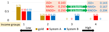
Figure 1. An example situation where the target distribution emphasises low-income groups and the distributions achieved by Systems A and B are being evaluated.

We address the problem of evaluating ranked lists based on group fairness (Ekstrand et al., 2021), given a target distribution over attribute values in each attribute set. Consider a hypothetical situation where we want a group-fair ranking of people, say, scholarship applicants. Suppose that the applicants are classified into four classes that represent their income levels (i.e., our attribute values), and that ideally, we want 75% of the ranking to represent the lowest income group, and the other 25% to represent the second lowest income group. As the user scans the ranked list of applicants, the list yields a series of achieved distributions over the four classes, based on the group membership of the item (i.e., income group of the applicant) at each rank. To measure the similarity between each achieved distribution and the gold distribution, we consider utilising ordinal quantification measures, namely, NMD (Normalised Match Distance, a normalised version of Earth Mover’s Distance (Werman et al., 1985)) and RNOD (Root Normalised Order-aware Divergence (Sakai, 2020)), in addition to a nominal quantification measure, namely, JSD (Jensen-Shannon Divergence) (Lin, 1991). Ordinal quantification measures take the ordinal nature of the attribute values into account, and may be appropriate for some applications. For example, consider the situation shown in Figure 1. While nominal quantification measures such as JSD say that Systems A and B are equally effective, NMD and RNOD say that B is better, as B is leaning more towards the lower income groups (25% is given to Group 3 rather than Group 4).

Our main contributions are as follows. (1) We present a simple and versatile framework for evaluating ranked lists in terms of group fairness and relevance, where the groups (i.e., possible attribute values) can be either nominal or ordinal in nature. (2) We demonstrate that, if the attribute set is binary (e.g., positive vs. negative opinions), our framework can easily quantify the overall polarity of each ranked list. (3) By utilising an existing diversified search test collection and treating each intent as an attribute value, we demonstrate that our framework can handle soft group membership (i.e., each ranked item can have multiple attribute values), and that our group fairness measures are highly correlated with both adhoc IR and diversified IR measures under this setting. (4) We demonstrate how our framework can quantify intersectional group fairness (Foulds et al., 2019) based on multiple attribute sets.

2. Related Work

Sections 2.1-2.4 discuss prior art that are highly relevant to our own group fairness evaluation framework. Here, we briefly mention prior art that these subsections do not cover. The group-fair ranking measures proposed in Kuhlman et al. (Kuhlman et al., 2019) assume the existence of a gold fair ranking, and are computed based on concordant and discordant pairs of ranked items by comparing the gold and system rankings. Their work focussed on binary attribute sets (i.e., protected vs. non-protected groups). See also Kuhlman et al. (Kuhlman et al., 2021) for a comparative study of measures under the binary setting. Raj et al. (Raj et al., 2020) compared single-ranking measures of Yang and Stoyanovich (Yang and Stoyanovich, 2017) and of Sapiezynski et al. (Sapiezynski et al., 2019) (which we discuss in Sections 2.1 and 2.2, respectively) as well as measures designed for distributions and sequences of rankings (Biega et al., 2018, 2020; Biega et al., 2021; Diaz et al., 2020; Singh and Joachims, 2018). The latter class of measures is beyond the scope of our work, as we are interested in evaluating a single ranked list when the target distribution over attribute values for each attribute set is given, either top-down (e.g., requiring a uniform distribution over all attribute values) or as a result of some bottom-up derivation (e.g., requiring statistical parity (Ekstrand et al., 2021) based on statistics from the target corpus). Also beyond our scope are the following lines of research: Beutel et al. (Beutel et al., 2019) propose to evaluate group fairness in the context of personalised recommendation by collecting pairwise item preferences from each user (See also Narasimhan et al (Narasimhan et al., 2020)); Kirnap et al. (Ömer Kirnap et al., 2021) estimate fair ranking measure scores from incomplete group membership labels.

2.1. Normalised Discounted KL Divergence

Geyik et al. (Geyik et al., 2019) considered two approaches to evaluating a ranked list of items (e.g., people), where the ranked list is expected to reflect as faithfully as possible a given target distribution over possible attribute values (e.g., female, male, other) in an attribute set (e.g., Gender), or over combinations of attribute values from multiple attribute sets (e.g., Gender AND Age Group). Let $A=\{a_{i}\}$ denote an attribute set. Their first proposal is a set retrieval measure for the top-$k$ search results, and is computed for a particular attribute value. For a given query, let $p_{\ast}(a_{i})$ denote the desired proportion of items having attribute value $a_{i}$ in the ranked list, s.t. $\sum_{i}p_{\ast}(a_{i})=1$. That is, $p_{\ast}$ is the gold probability mass function over $A$. Let $L$ denote a ranked list, and let $L@k$ denote its top-$k$ portion. Let $p_{L@k}(a_{i})$ be the actual proportion of items having attribute value $a_{i}$ within the top-$k$ results, s.t. $\sum_{i}p_{L@k}(a_{i})=1$. That is, $p_{L@k}$ is the achieved probability mass function over $A$. The Skew for $a_{i}$ is defined as $\textit{Sk}(a_{i},L@k)=\log_{\mathrm{e}}(p_{L@k}(a_{i})/p_{\ast}(a_{i}))$. Although Geyik et al. point out that situations where $p_{\ast}(a_{i})=0$ should be avoided, note that $p_{\ast}(a_{i})=0$ may well happen in practice, especially if combinations of multiple attribute sets are considered (e.g., Gender=“male” AND Age=“$x>90$” AND $\ldots$). They also propose to utilise $\max_{i}{\it Sk}(a_{i},L@k)$ and $\min_{i}{\it Sk}(a_{i},L@k)$ to discuss the quality of the top-$k$ results with respect to the attribute set $A$. However, it is clear that the skew-based measures focus only on the worst-case and best-case attribute values. In summary, skew-based measures are not adequate for our purpose because (a) they cannot handle ranked retrieval; and (b) they do not consider every attribute value in $A$ (when $|A|>2$); and (c) $p_{\ast}(a_{i})=0$ can cause inconveniences.

The second proposal by Geyik et al. was to slightly modify a ranked retrieval measure of Yang and Stoyanovich (Yang and Stoyanovich, 2017), called rKL. The modified measure, which Geyik et al. refer to as Normalised Discounted KL divergence (NDKL), utilises the Kullback-Leibler Divergence (KLD) to compare the achieved and gold distributions.

(1) $${\it NDKL}(L)=\frac{\sum_{k=1}^{|L|}\left(\sum_{i}p_{L@k}(a_{i})\textit{Sk}(a_{i},L@k)\right)/\log_{2}(k+1)}{\sum_{k=1}^{|L|}1/\log_{2}(k+1)}\ .$$

Note that NDKL overcomes Limitations (a) and (b) mentioned above, but not (c), since it is based on Skew. Yet another inconvenience with KLD is: (d) it is unbounded. We prefer to use Jensen-Shannon Divergence (JSD) instead as it solves Limitations (c) and (d); Draws et al. (Draws et al., 2021) and the TREC 2021 Fair Ranking Track has also adopted JSD. Furthermore, as we have mentioned in Section 1, our proposed framework offers ordinal quantification measures as possible alternatives to nominal quantification measures such as JSD.

Geyik et al. (and Ghosh et al. (Ghosh et al., 2021a, b)) argue that intersectional group fairness (Foulds et al., 2019) can be handled by considering combined attribute values from multiple attribute sets, such as SkinType AND Gender (Buolamwini and Gebru, 2018). However, we argue that this may not be the best approach to take if both nominal and ordinal attribute values need to be considered and if it seems appropriate to take the ordinal nature of the attribute values into account. For example, consider combining Gender (nominal) and Age Group (ordinal), and a combined attribute value Gender=“female” AND Age=“$x<20$.” Which of the following two combined attribute values is closer to the above, Gender=“male” AND Age=“$20\leq x<40$” (Gender: incorrect; Age Group: not far off) or Gender=“female” AND Age=“$40\leq x<60$” (Gender: correct; Age Group: far off)? Similar problems arise when multiple ordinal classes are combined. Hence, for applications where ordinal quantification measures seem more appropriate than nominal ones such as JSD, we propose to compare the achieved and gold distributions for each attribute set at a time, and finally aggregate the scores across the multiple attribute sets.

NDKL adopted the log-based discounting scheme of nDCG (Järvelin and Kekäläinen, 2002; Sakai, 2014) because “it is more beneficial for an item to be ranked higher, it is also more important to achieve statistical parity at higher ranks.” The discounting scheme can be interpreted as reflecting user attention over a ranked list. However, Ghosh et al. (Ghosh et al., 2021a) and Sapiezynski et al. (Sapiezynski et al., 2019) argue that the log-based decay is too fat-tailed for modelling user attention. The next section reviews their work.

2.2. Expected Cumulative Exposure

Inspired by the work of Sapiezynski et al. (Sapiezynski et al., 2019) that considered user attention over search results, Ghosh et al. (Ghosh et al., 2021a) presented a group fairness measure called Attention Bias Ratio (ABR). Let $F_{L@k}(a_{i})=1$ if the item at rank $k$ in ranked list $L$ has attribute value $a_{i}$, and let $F_{L@k}(a_{i})=0$ otherwise. The Mean Attention (MA) score of $a_{i}$ for $L$ is defined as:

(2) $${\it MA}(a_{i},L)=\frac{\sum_{k=1}^{|L|}F_{L@k}(a_{i})\,\,{\it Attention}_{p}@k}{\sum_{k=1}^{|L|}F_{L@k}(a_{i})}\ ,$$

where ${\it Attention}_{p}@k=100p(1-p)^{k-1}$, which is essentially the decay function of Rank-Biased Precision (RBP) for a given patience parameter value $\phi=1-p$ (Moffat and Zobel, 2008). Note that this decay depends entirely on the document rank; it considers neither relevance nor fairness of the documents seen so far. This limitation applies to NDKL (Eq. 1) as well. Hence, if relevance assessments are available, we use the cascade-based decay of Expected Reciprocal Rank (ERR) (Chapelle et al., 2011) as in Biega et al. (Biega et al., 2020; Biega et al., 2021) and Diaz et al. (Diaz et al., 2020).

Ghosh et al. (Ghosh et al., 2021a) define ABR as:

(3) $${\it ABR}(L)=(\min_{a_{i}\in A}{\it MA}(a_{i},L))/(\max_{a_{i}\in A}{\it MA}(a_{i},L))\ .$$

Thus, ABR quantifies the disparity between the attribute values with lowest and highest mean attention scores. It is clear that Limitation (b) mentioned in Section 2.1 applies to this measure as well. In contrast, our group fairness framework considers every attribute value in each attribute set.

In Eq. 2, note that $F_{L@k}(a_{i})$ is a group membership flag, representing hard group membership. However, in the original work of Sapiezynski et al. (Sapiezynski et al., 2019), group membership is formulated as a probability mass function over the attribute values (i.e., soft group membership). That is, let $G_{L@k}(a_{i})$ be the probability that the item at rank $k$ in $L$ has attribute $a_{i}$, s.t. $\sum_{i}G_{L@k}(a_{i})=1$. If the group membership probability mass function $G_{L@k}$ is available for each $k$, then $G_{L@k}(a_{i})$ can replace $F_{L@k}(a_{i})$ in Eq. 2. For ranked list $L$, Sapiezynski et al. (Sapiezynski et al., 2019) compute a probability distribution over $A$ called the expected cumulative exposure (ECE), where the probability for $a_{i}$ is given by

(4) $$E_{L}(a_{i})=\sum_{k=1}^{|L|}G_{L@k}(a_{i})\,\,{\it Attention}_{p}@k\ .$$

Note that this generalises the numerator of Eq. 2. Sapiezynski et al. propose to compare $E_{L}$ with the gold probability mass function $p_{\ast}$ by assuming that both $E_{L}$ and $p_{\ast}$ are binomial distributions, and conduct a form of statistical significance test with a test statistic threshold to discuss whether a ranked list is fair or not. In contrast, we are more interested in quantifying the degree of group fairness of a ranked list rather than binary classification, and do not rely on any distributional assumptions. As we shall demonstrate in Section 4.2, our framework can also handle soft group membership, which is important not only for situations where each ranked item can take multiple attribute values, but also for situations where the group membership of each item needs to be estimated with some degree of uncertainty.

2.3. Polarity on a Binary Attribute Set

Consider a situation with a single binary attribute set, $A=\{a_{1},a_{2}\}$, e.g., Democrats vs. Republicans (Kulshrestha et al., 2017; Robertson et al., 2018). Suppose that, for each item at rank $k$ in ranked list $L$, its bias score $b_{L@k}$ is available (Robertson et al., 2018), whose range is $[-1,1]$; a negative score means leaning towards $a_{1}$, a positive score means leaning towards $a_{2}$, and 0 means neutral. Kulshrestha et al. (Kulshrestha et al., 2017) proposed the Output Bias (OB) measure, which is an average-precision-like measure based on bias scores. Whereas OB is only applicable to binary attribute sets, our framework can handle any number of attribute values. If bias scores are available (Robertson et al., 2018) in a binary setting, our framework can leverage them by converting them to group membership probabilities as follows.

(5) $$G_{L@k}(a_{1})=(1+b_{L@k})/2\ ,\,\,\,G_{L@k}(a_{2})=1-G_{L@k}(a_{1})\ .$$

Experimental validation of the above method is left for future work.

Gezici et al. (Gezici et al., 2021) also proposed methods to quantify bias in SERPs (Search Engine Result Pages) in a binary setting, where the objective is to achieve equality of outcome, i.e., $p_{\ast}(a_{1})=p_{\ast}(a_{2})=1/2$. They point out that measures like NDKL (Eq. 1) cannot tell whether a SERP is biased towards $a_{1}$ and $a_{2}$, and propose to compute a (weighted) average of the polarity value ($F_{L@k}(a_{1})-F_{L@k}(a_{2})$) across document ranks, where $F$ is a group membership flag as before (See Eq. 2), but returns 1 only when the document at $k$ belongs to the group in question and is relevant. In Section 4.1, we demonstrate that our framework can easily quantify the overall polarity of each ranked list given a binary attribute set.

2.4. Diversity Evaluation Measures

Cherumanal et al. (Cherumanal et al., 2021) applied the measures proposed by Yang and Stoyanovich (Yang and Stoyanovich, 2017) as well as a diversified search evaluation measure ($\alpha$-nDCG (Clarke et al., 2011)) to evaluate the Touché 2020 argument retrieval runs from CLEF 2020 (Bondarenko et al., 2020); they observed that systems are generally ranked differently by fairness, diversity, and relevance measures. Diaz et al. (Diaz et al., 2020) discussed the connection between group fairness measures (for a distribution of ranked lists) and intent-aware diversity measures (Agrawal et al., 2009; Chapelle et al., 2011; Sakai, 2014). On the other hand, for diversity evaluation, Sakai and Song (Sakai and Song, 2011, Table 7) demonstrated a few advantages of their D$\sharp$-measures over $\alpha$-nDCG and intent-aware measures; Sakai and Zeng (Sakai and Zeng, 2020) reported that an instance of the D$\sharp$-measure called D$\sharp$-nDCG outperformed intent-aware measures in terms of how the measure agrees with human SERP preferences.

Zehlike et al. (Zehlike et al., 2017) remarked that D$\sharp$-nDCG can be applied to group-fair ranking evaluation by treating their binary attribute set (protected/non-protected) as two search intents behind the same query. We generalise this idea and use D$\sharp$-nDCG as the representative of existing diversity measures in our experiments to see how group-fair and diversified ranking evaluations are related given either hard or soft group membership. D$\sharp$-nDCG is the average of intent recall (a.k.a. subtopic recall (Zhai et al., 2003)) and D-nDCG (Sakai and Song, 2011); the difference between the standard nDCG (for adhoc IR) and D-nDCG (for diversified IR) is that the latter is based on the global gain of each document $d$:

(6) $$\textit{GG}(d)=\sum_{i\in I_{q}}\textit{Pr}(i\mid q)g_{i}(d)\ ,$$

where $I_{q}$ is the set of known intents for topic $q$, $\textit{Pr}(i\mid q)$ is the probability that a user who enters $q$ as a query has Search Intent $i$, and $g_{i}(d)$ is the gain value of $d$ for Intent $i$. From Eq 6, it can be observed that if the intent probabilities are uniform and the attribute values are mutually exclusive (i.e., hard group membership is defined), the global gain reduces to a single gain value and therefore that D-nDCG reduces to the standard nDCG. This is exactly the situation in our first experiment (Section 4.1), as it uses the aforementioned Touché 2020 data: each ranked item (i.e., opinion) is either PRO or CON, but not both.

3. Proposed Evaluation Framework

Our premise is that we are given $M$ attribute sets, where the $m$-th attribute set is $A^{m}(m=1,\ldots,M)$ with $i$ specifying a particular attribute value $a_{i}^{m}(\in A^{m})$. For each $A^{m}$, we are also given a target distribution $p_{\ast}^{m}$ over its attribute values, s.t. $\sum_{i}p_{\ast}^{m}(a_{i}^{m})=1$. An example setting with $M=2$ would be $p_{\ast}^{\mathrm{Gender}}(\mathrm{female})=p_{\ast}^{\mathrm{Gender}}(\mathrm{male})=p_{\ast}^{\mathrm{Gender}}(\mathrm{other})=1/3,p_{\ast}^{\mathrm{Age}}(x<20)=p_{\ast}^{\mathrm{Age}}(\mathrm{x\geq 80})=0.2,p_{\ast}^{\mathrm{Age}}(20\leq x<80)=0.6$. Given these targets, we are also given a ranked list $L$ to evaluate, where each item at rank $k$ has a group membership probability $G_{L@k}(a_{i}^{m})$ s.t. $\sum_{i}G_{L@k}(a_{i}^{m})=1$ for every $k$. (Recall that group membership flag $F_{L@k}$ is a special case of $G_{L@k}$.) If the item at rank $k$ does not correspond to any of the attribute values of $A^{m}$, we let $G_{L@k}(a_{i}^{m})=1/|A^{m}|$. That is, we assume that the distribution over the attribute values is uniform for that item. Our objective is to quantify how well $L$ aligns with the target distributions and, if relevance assessments are also available, evaluate $L$ in terms of both group fairness and relevance.

For each attribute set, we can evaluate the group fairness of $L$ as:

(7) $$\textit{GF}^{m}(L)=\sum_{k=1}^{|L|}\textit{Decay}_{L@k}^{m}\,\,\,\textit{DistrSim}_{L@k}^{m}\ ,$$

where $\textit{Decay}_{L@k}^{m}$ is a function that represents the user attention decay as they go down the ranked list, and $\textit{DistrSim}_{L@k}^{m}$ compares the achieved distribuiton $p_{L@k}^{m}$ with the target distribution $p_{\ast}^{m}$. In the present study, we employ the relevance-based decay of ERR (Chapelle et al., 2009; Diaz et al., 2020) by default, as we view this user model to be more realistic than those of nDCG and RBP that disregard item relevance. That is,

(8) $$\textit{Decay}_{L@k}=P_{L@k}^{\mathrm{rel}}\prod_{j=1}^{k-1}(1-P_{L@j}^{\mathrm{rel}})\,\,\,\,\,\,\,(k>1)$$

and $\textit{Decay}_{L@1}=P_{L@1}^{\mathrm{rel}}$, where $P_{L@k}^{\mathrm{rel}}=(2^{g}-1)/2^{g}$ if the relevance grade of the item ranked at $k$ is $g$ (Chapelle et al., 2009). Note that we have removed the $m$ from Eq. 8 as the present study assumes that group membership for a particular attribute set does not affect attention decay. While “group fairness seen so far” may well affect the user attention decay just like “relevance seen so far,” this consideration is left for future work. When relevance assessments are unavailable, we employ the RBP-based decay instead: $\textit{Decay}_{L@k}=(1-\phi)\phi^{k-1}$ with $\phi=0.85$. This is equivalent to assuming that $P^{\mathrm{rel}}_{L@k}=0.15$ for any $L$ and $k$ when computing Eq. 8.

For each rank $k$ in $L$, the achieved distribution $p_{L@k}^{m}$ is computed by letting $p_{L@k}(a_{i}^{m})=\sum_{j=1}^{k}G_{L@j}(a_{i}^{m})/k$. This is the average group membership probability over top $k$ for attribute value $a_{i}^{m}$. As for $\textit{DistrSim}_{L@k}^{m}$, we consider different functions for comparing $p_{L@k}^{m}$ with $p_{\ast}^{m}$ depending on whether the attribute values are nominal or ordinal and, in the latter case, whether considering the ordinal nature of the attribute values makes sense (See Section 1). More specifically, given an achieved and the gold probability mass functions $p$ and $p_{\ast}$, we consider the following options.

(9) $$\textit{DistrSim}(p\parallel p_{\ast})=1-\textit{Divergence}(p\parallel p_{\ast})\ ,$$

where $\textit{Divergence}(p\parallel p_{\ast})$ is either JSD, NMD, or RNOD (See Section 1); we use notations such as $\textit{DistrSim}^{\mathrm{JSD}}$ where appropriate. Note that JSD should be used for nominal attribute sets unless the attribute set is binary; for binary attribute sets, any of the above divergences can be used as there is no distinction between nominal and ordinal scales. In fact, as Sakai (Sakai, 2021a) shows that NMD and RNOD are the same when $A^{m}=\{a_{1},a_{2}\}$, we have two options for the binary case: JSD and NMD (i.e., RNOD).

Given $M$ attribute sets, we predefine a set of weights $w_{0},w_{1},\ldots,w_{M}$ s.t. $\sum_{m=0}^{M}w_{m}=1$, and compute the overall score of $L$ as a weighted average. We call it the GFR (Group Fairness and Relevance) score.

(10) $$\textit{GFR}(L)=w_{0}\textit{Relevance}(L)+\sum_{m=1}^{M}w_{m}\textit{GF}^{m}(L)\ ,$$

where $\textit{Relevance}(L)$ is a relevance-based score; we let $w_{0}=0$ if relevance assessments are unavailable. In either case, the present study only considers unweighted versions of Eq. 10, and leaves the question of how $w_{m}$’s should be set for future work. As for the choice of $\textit{Relevance}(L)$, we consider ERR and iRBU (intentwise Rank-Biased Utility) (Sakai and Zeng, 2020; Sakai, 2021b) because these measures also rely on the realistic decay function given by Eq. 8 and therefore enable us to rewrite Eq. 10 as follows.

(11) $$\sum_{k=1}^{|L|}\textit{Decay}_{L@k}\left(w_{0}\textit{Utility}_{L@k}+\sum_{m=1}^{M}w_{m}\textit{GF}^{m}_{L@k}\right)\ ,$$

where $\textit{Utility}_{L@k}=1/k$ for ERR and $\textit{Utility}_{L@k}=\phi^{k}$ for iRBU. Whereas ERR is suitable for navigational searches, iRBU is a measure that behaves surprisingly similarly to nDCG (Sakai and Zeng, 2020; Sakai, 2021b) and is more geared towards informational searches. Eq. 11 implies a user model which says that the user is scanning down the ranked list while experiencing a sequence of documents with different relevance levels and a gradually changing distribution over the attribute values for each attribute set. However, as was mentioned earlier, our current decay component considers relevance only.

4. Experiments with Real Data

This section demonstrates the versatility of our group fairness evaluation framework through three case studies with real data. Hereafter, we consider evaluating the top $|L|=10$ items of any given ranked list. All relevance-based measures are computed based on an exponential gain value setting. That is, a gain value of $2^{g}-1$ is given to each $g$-relevant document ($g=0,1,2\ldots$).

4.1. Ranking Pros and Cons: Quantifying the Polarity with One Binary Attribute Set

As a case study of a ranking task with a binary attribute set, we follow Cherumanal et al. (Cherumanal et al., 2021) and utilise the Touché 2020 Data from CLEF 2020 (Bondarenko et al., 2020). The task used the args.me corpus (Ajjour et al., 2019), which is a collection of opinions each tagged with either PRO ($a_{1}$) or CON ($a_{2}$). We use Version 1 of args.me, with the Version 1 qrels file from Touché 2020 (containing 2,964 topic-document pairs, covering 49 topics), and the 21 submitted runs. The qrels file offers graded relevance on a 6-point scale: $g=1,\ldots,5$ along with $-2$ (non-arguments). We treat the non-argument documents as nonrelevant ($g=0$). Although the runs were evaluated only in terms of relevance at Touché 2020, we computed the GFR scores using GF^JSD (group fairness), ERR and iRBU (relevance); hence the GFR measures are denoted by ERR+GF^JSD and iRBU+GF^JSD. For now, let us consider a flat setting, where the target distribution is $p_{\ast}(\mathrm{PRO})=p_{\ast}(\mathrm{CON})=0.5$. In addition, we also compute D$\sharp$-nDCG using the NTCIREVAL toolkit by treating PRO and CON as two search intents behind a query and treating the combination of the relevance level and the PRO/CON label for each document as a per-intent relevance label. As for intent probabilities, we also use a uniform distribution: $\textit{Pr}(\mathrm{PRO}\mid q)=\textit{Pr}(\mathrm{CON}\mid q)=0.5$ (See Eq. 6). Note that, as we are dealing with hard group membership in this experiment, D$\sharp$-nDCG reduces to an average of intent recall and the standard nDCG (See Section 2.4).

Table 1 compares the run rankings of different measures under the flat setting using Kendall’s $\tau$. It can be observed that:

• GF^JSD is only moderately correlated with ERR, iRBU, and D$\sharp$-nDCG ($\tau=$0.438-0.667), which suggests that group fairness evaluation is related to but different from adhoc and diversity evaluations, at least in a hard group membership setting with a binary attribute set. This high-level observation is in line with the results of Cherumanal et al. (Cherumanal et al., 2021) who also used the Touché 2020 data to compare NKDL, nDCG, and $\alpha$-nDCG.

• The GFR measures (i.e., {ERR, iRBU}+GF^JSD) are more highly correlated with D$\sharp$-nDCG ($\tau=$0.800-0.867) than GF^JSD is. That is, a combination of a group fairness measure and a relevance measure is relatively similar to a diversity measure (which actually is the average of intent recall and nDCG in this experiment).

Table 1. System ranking correlations (Kendall’s $\tau$ with 95%CIs) for the 21 Touché 2020 runs.

	ERR	iRBU	ERR+GFJSD	iRBU+GFJSD	D$\sharp$-nDCG
GFJSD	0.438	0.667	0.552	0.829	0.648
	[0.154, 0.655]	[0.455, 0.807]	[0.298, 0.733]	[0.702, 0.905]	[0.428, 0.795]
ERR	-	0.771	0.886	0.610	0.790
		[0.610, 0.871]	[0.796, 0.938]	[0.375, 0.771]	[0.639, 0.882]
iRBU	-	-	0.886	0.838	0.867
			[0.796, 0.938]	[0.716, 0.910]	[0.764, 0.927]
ERR+GFJSD	-	-	-	0.724	0.867
				[0.538, 0.843]	[0.764, 0.927]
iRBU+GFJSD	-	-	-	-	0.800
					[0.655, 0.888]

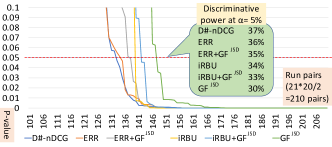
Figure 2. Discriminative power curves based on the randomised Tukey HSD test (Touché 2020 runs).

Figure 2 shows the discriminative power curves (Sakai, 2007, 2014) of the measures for the 21 Touché runs (210 run pairs) based on a randomised Tukey HSD test (Sakai, 2018) with 5,000 trials conducted with the Discpower tool. For example, D$\sharp$-nDCG is the most discriminative (with 78 statistically significantly different run pairs out of 210 comparisons, i.e., 37%) at the 5% significance level. When we look at the actual significance test results at the 5% significance level (i.e., the raw results used to draw Figure 2), a run called WeissSchnee-1 is the top performer in terms of D$\sharp$-nDCG: this is the only run that outperforms 7 other runs. On the other hand, in terms of statistical significance with ERR, iRBU, and GF^JSD, there are 4, 17, and 14 runs tied at the top; WeissSchnee-1 is in the highest performing cluster for all three measures, and its rank in terms of mean scores is 1, 2, and 8, respectively. That is, WeissSchnee-1 is only the 8th-best among the 21 runs in the ranking according to mean GF^JSD. This example also suggests that group fairness evaluation is not the same as relevance and diversity evaluations, at least in a hard group membership setting with a binary attribute set.

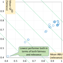
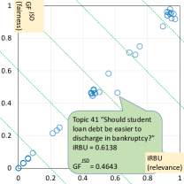
Figure 3. Visualising the mean group fairness and relevance scores of the 21 Touché runs (over 49 topics).

Figure 4. Visualising the per-topic scores of the lowest performer from Figure 4. The Kendall’s $\tau$ between iRBU and GF^JSD for this run is 0.867 (95%CI[0.810, 0.908], $n=49$).

Figure 4 visualises how the iRBU-based and GF^JSD-based run rankings are correlated ($\tau=0.667$ as shown in Table 1). We stress that it is important to visualise the runs in this way to complement a list of runs ranked by GFR scores (Eq. 10), so that we can see how the GF and relevance components are contributing to GFR. The dotted lines represent contour lines in terms of GFR (i.e., iRBU+GF^JSD). Figure 4 visualises the per-topic iRBU and GF^JSD scores for the lowest performer indicated in Figure 4: as shown with a baloon in Figure 4, we can easily spot SERPs that are relatively poorly balanced between group fairness and relevance in this way.

We now demonstrate how our framework can quantify the polarity of runs, i.e., whether the runs are biased towards PRO or towards CON, and by how much. Instead of the flat setting that we considered earlier, let us consider a 100% PRO setting ($p_{\ast}(\mathrm{PRO})=1,p_{\ast}(\mathrm{CON})=0$) and a 100% CON setting ($p_{\ast}(\mathrm{PRO})=0,p_{\ast}(\mathrm{CON})=1$). Let $\textit{GF}_{\mathrm{PRO}}(L)$ and $\textit{GF}_{\mathrm{CON}}(L)$ denote a GF score for ranked list $L$ computed under the two settings, respectively. Then $\Delta\textit{GF}(L)=\textit{GF}_{\mathrm{PRO}}(L)-\textit{GF}_{\mathrm{CON}}(L)$ is a direct measure of the polarity of $L$: a positive score implies an overall bias towards PRO, and so on. Note that replacing the target distribution affects only the DistrSim part of Eq. 7.

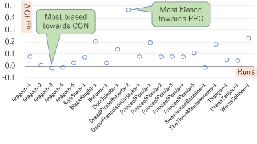
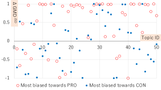
Figure 5. Quantifying the polarity of the Touché 2020 runs ($x$-axis) using Mean $\Delta\textit{GF}$ ($y$-axis) over 49 topics.

Figure 6. Per-topic $\Delta\textit{GF}^{\mathrm{NMD}}$ scores for the two most biased runs from Figure 6.

Figure 6 compares the mean $\Delta\textit{GF}^{\mathrm{JSD}}$ scores of the 21 Touché 2020 runs. With the exception of the three runs shown only slightly below the $x$-axis, it can be observed that the runs are generally biased towards PRO. Figure 6 examines the per-topic $\Delta\textit{GF}^{\mathrm{JSD}}$ scores for the two most extreme runs indicated in Figure 6: it can be observed that the most PRO-biased run is almost completely biased towards PRO for many topics (with 37 topics above the $x$-axis), while the most CON-biased run is much more well-balanced (with 23 and 26 topics above and below the $x$-axis, respectively).

We have thus demonstrated that our evaluation framework is applicable to a hard group membership setting with a binary attribute set where both group fairness and relevance need to be considered, and that our framework can quantify the polarity of each run as well as each ranked list in a straightforward manner.

4.2. Ranking Web Pages: Soft Group Membership with One Attribute Set

We now demonstrate that our framework can handle soft group membership, i.e., probabilities $G_{L@k}(a_{i})$ rather than flags $F_{L@k}(a_{i})$ like PRO/CON. To this end, we utilise a diversified search data set from the NTCIR-9 INTENT Japanese subtask data (Song et al., 2011). We chose the NTCIR data over the TREC diversity task data (Clarke et al., 2013) because (a) an NTCIR INTENT task data set (with associated runs) contains 100 topics (with 3-24 intents per topic) while a TREC diversity data set contains only 50; and more importantly, (b) unlike the TREC data, the NTCIR data contains intent probabilites based on assessors’ majority votes. In our experiments, we directly utilise these intent probabilities to define the target distribution in the group fairness context, by treating the search intents for each topic as attribute values. For example, Topic 0127 “Mikuniya” (a Japanese proper name) is an ambiguous topic, because it can be a famous Japanese tea shop, a restaurant, a hot springs resort, and so on; these are all different entities; the tea shop intent has a 37% probability according to the INTENT data, and we use this directly as the gold probability for group fairness evalution. Thus, while search result diversification aims to satisfy many users with different intents behind the query Mikuniya, we view the problem in a group fairness context where we want to make sure that we are giving a fair exposure to each entity named Mikuniya.

In the INTENT data, a single document may be relevant to multiple intents and therefore soft group membership needs to be handled. For example, for “Mikuniya,” there are five documents that are relevant to as many as six intents. We define the soft group membership for an item based on its per-intent gain values: if there are three intents and the item has 3, 1, 0 as its per-intent gain values, the group membership is distributed across the intents as $3/4,1/4,0$. To compute the ERR-based decay (Eq. 8), we utilise the per-topic relevance grades available from Sakai and Zeng (Sakai and Zeng, 2020), which were derived from the official per-intent relvance assessments. Along with GF^JSD-based GFR measures, we also compute D$\sharp$-nDCG, the official diversity measure used in the INTENT task. Recall that D$\sharp$-nDCG utilises the intent probabilities as shown in Eq. 6.

Table 2. System ranking correlations (Kendall’s $\tau$ with 95%CIs) for the 18 INTENT runs.

	ERR	iRBU	ERR+GFJSD	iRBU+GFJSD	D$\sharp$-nDCG
GFJSD	0.843	0.791	0.908	0.882	0.895
	[0.709, 0.918]	[0.622, 0.890]	[0.824, 0.953]	[0.777, 0.939]	[0.801, 0.946]
ERR	-	0.895	0.935	0.935	0.869
		[0.801, 0.946]	[0.874, 0.967]	[0.874, 0.967]	[0.754, 0.932]
iRBU	-	-	0.882	0.908	0.817
			[0.777, 0.939]	[0.824, 0.953]	[0.665, 0.904]
ERR+GFJSD	-	-	-	0.974	0.882
				[0.949, 0.987]	[0.777, 0.939]
iRBU+GFJSD	-	-	-	-	0.856
					[0.731, 0.925]

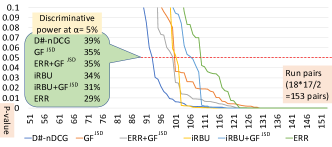
Figure 7. Discriminative power curves based on the randomised Tukey HSD test (INTENT runs).

Using Kendall’s $\tau$, Table 2 compares the rankings of the 21 INTENT runs according to different measures. Recall that, unlike Table 1, we are dealing with soft group membership with 3-24 intents (i.e., attribute values) per topic. It can be observed that our GF and GFR measures are all highly correlated with the offcial diversity measure, i.e., D$\sharp$-nDCG. Interestingly, GF^JSD is slightly more highly correlated with D$\sharp$-nDCG than the relevance-based measures (i.e., ERR and iRBU) are, although the differences are not statistically significant according to the 95%CIs. This suggests that, at least in some search scenarios with soft group membership, group-fair ranking (for stakeholders of the ranked items) and search result diversification (for search engine users) may be two sides of the same coin, or at least, of two similar coins. This is in contrast to Cherumanal et al. (Cherumanal et al., 2021) and the experiments in Section 4.1 where hard group membership with a binary attribute set was considered. One possible cause for the high correlation between GF and D$\sharp$-nDCG is that we have assumed that the target distribution for group fairness (See Eq. 9) and the probability distribution of intents given a topic (See Eq. 6) are one and the same. In practice, they may well differ, in which case GF and D$\sharp$-nDCG may possibly give us substantially different results.

Figure 7 shows the discriminative power curves of the measures for the 18 INTENT runs (153 run pairs). The most discriminative measure is D$\sharp$-nDCG, which is consistent with Figure 2. However, for the INTENT data set, it can be observed that GF^JSD is at least as discriminative as ERR and iRBU. When we examine the raw significance test results at $\alpha=0.05$, D$\sharp$-nDCG says that four runs (MSINT-D-J-{3,1,2,4}) are tied at the top, statistically significantly outperforming 7 other runs. As for GF^JSD, it says that MSINT-D-J-3 is the top performer, as it is the only run that statistically significantly outperforms 8 other runs. In terms of mean scores, all measures except iRBU agree that MSINT-D-J-3 is the most effective among the 18 runs; the ranking by mean iRBU says that this run is the third best.

We have thus demonstrated that our framework can handle soft group membership, and that GF^JSD (group fairness) and D$\sharp$-nDCG (diversity and relevance) are highly correlated under this setting.

4.3. Ranking Local Shops and Restaurants: Intersectional Group Fairness

Our third case study involves two attribute sets, one with nominal attribute values and the other with ordinal attribute values (but without relevance data). The purpose of this experiment is to show that (i) unlike prior art, our framework can consider the ordinal nature of the attribute values if required; (ii) for handling ordinal attribute values, the choice of the DistrSim function (Eq. 9) matters in some cases; and (ii) intersectional group fairness of rankings can be examined without directly combining different attribute sets.

For this experiment, we constructed a data set based on a query log from a popular Local Shop and Restaurant Search service for smartphone users in Japan. Given a query, this Local Search service returns a ranked list of items (i.e., shops and restaurants) based on various features including the relevance to the query, the proximity of the item to the user’s location, and user ratings (i.e., review scores). In our query log, each ranked item has a flag indicating whether it is a chain store owned by a company, and if it is, the name of the company that owns it. For some queries, a small number of companies that own many chain stores may dominate the ranking. Hence, as an example of imposing a group fairness requirement based on a nominal attribute set (with hard group membership), we require, for each query, that the ideal ranking should provide the same exposure to all relevant companies. More specifically, the gold distribution is defined as a uniform distribution over all companies that appear in the top 20 ranking (based on the current Local Search results) for that query, where each shop or restaurant that is not a chain store is treated as a distinct company. In order to demonstrate that our framework can evaluate group fairness from the above viewpoint, we first obtained a random sample from a one-year Local Search query log (from September 2020 to September 2021), and then filtered it so that each ranking contains at least one company with multiple chain stores listed in the top 20. This gave us a set of 418 queries for our experiment.

Our query log also contains a mean 5-point scale user rating score and a review count for each item. If an item has $n(>0)$ reviews, the mean rating is the average over $n$ user ratings; if there is no review, the mean rating is set to zero. We believe that imposing a group fairness requirement based on review count is of practical significance, because this statistic probably reflects the level of exposure of each item in the past, and items with low past exposure may deserve more future exposure. Hence, as an example of handling an ordinal attribute set (with hard group membership), we consider a group fairness constraint based on this view. In the aforementioned query log (before filtering by chain store information), 45% of the ranked items had zero reviews (Group 1), 22% had 1-10 reviews (Group 2), 23% had 11-100 reviews (Group 3), and the remaining 10% had over 100 reviews (Group 4). We utilise this distribution as the gold distribution over the four review count groups for all queries, to demonstrate how this search application can be evaluated in terms of statistical parity (Ekstrand et al., 2021).

We evaluate the following four runs (i.e., ranking schemes) to demonstrate how our framework can handle a nominal attribute set and an ordinal attribute set at the same time and thereby enable us to quantify intersectional group fairness.

Base:

This represents the actual rankings returned by our current Local Search engine. The search engines leverages various features to produce the rankings as mentioned earlier, but it suffices to treat it as a black box for the purpose of the present experiment.

Rating:

This reranks the top 20 search results by the mean ratings from user reviews, so that items with higher ratings are prioritised. This is likely to affect the review count-based group fairness. For example, if many of the items with higher ratings are those that have already enjoyed good exposure to users and therefore received many reviews (i.e., there is a high correlation between mean rating and review count), Rating may underperform Base in terms of review count-based group fairness: recall that our gold distribution for review count groups allocates 45% to Group 1 (items with zero reviews). The actual Kendall’s $\tau$ between the mean ratings and the review counts based on all ranked items for the 418 queries ($n=9,329$ items) is 0.617 (95%CI[0.609, 0.625]); hence there is indeed a substantial positive correlation. On the other hand, note that even an item with only one review can have a mean rating of 5 (i.e., maximum); that is, ranking by mean rating is not the same as ranking by review count.

Base-UC:

Filter the top 20 items of the Base run so that each company (which can own multiple chain stores) appears no more than once. UC stands for “Unique Chain.” This is designed to improve the chain-based group fairness.

Rating-UC:

Similar to Base-UC, except that the input to the filtering step is the Rating run. This should also improve the chain-based group fairness of Rating.

Since relevance assessments are missing in this experiment, we use the RBP decay (See Section 3). For discussing the chain-based group fairness (where the number of nominal bins for the uniform gold distribution varies across topics), we compute GF^JSD. For discussing the review count-based group fairness (with a statistical parity-based gold distribution over 4 ordinal bins common to all topics), we compute GF^JSD, GF^NMD, and GF^RNOD. We shall denote these measures as chain-GF^JSD, revcnt-GF^NMD, etc.; we also average a chain-based score and a revcnt-based score as a special case of Eq. 10 with $w_{0}=0$ (i.e., doing without relevance) and $w_{1}=w_{2}=0.5$ (where $i=1,2$ represent the chain and revcnt attribute sets, respectively). We shall refer to the averages as intersectional measures and denote them by chain-GF^JSD+revcnt-GF^NMD and so on.

Table 3. Mean GF scores of the 4 Local Search runs (over 418 topics).

	chain-GFJSD	revcnt-GFJSD	revcnt-GFNMD	revcnt-GFRNOD
Base	0.404	0.495	0.542	0.460
Base-UC	0.479	0.545	0.575	0.500
Rating	0.401	0.445	0.551	0.422
Rating-UC	0.479	0.506	0.584	0.470

Table 4. Randomised Tukey HSD test results ($\alpha=0.05$) for Table 4. “$\gg$” means “statistically significantly better than.”

Measure	Conclusions
(a) 4 pairs with a statistically significant difference
chain-GFJSD,	Rating-UC $\gg$ Base, Rating
revcnt-GFNMD,	Base-UC $\gg$ Base, Rating
chain-GFJSD+revcnt-GFNMD
(b) 5 pairs with a statistically significant difference
revcnt-GFJSD,	Base-UC $\gg$ Rating-UC, Base, Rating
revcnt-GFRNOD	Rating-UC $\gg$ Rating
	Base $\gg$ Rating
(c) 6 pairs with a statistically significant difference
chain-GFJSD+revcnt-GFJSD,	Base-UC $\gg$ Rating-UC, Base, Rating
chain-GFJSD+revcnt-GFRNOD	Rating-UC $\gg$ Base, Rating
	Base $\gg$ Rating

Table 4 shows the mean GF scores of the 4 runs averaged over the 418 topics; intersectional measures are omitted here as they can easily be computed from the table. Table 4 summarises the significance test results for all 7 measures. Due to the large sample size ($n=418$), the differences shown in the table are all statistically highly significant ($p<0.003$). We can observe that:

• With all 7 measures, Base-UC statistically significantly outperforms Base, and Rating-UC statistically significantly outperforms Rating. That is, the Unique Chain filtering step improves not only the chain-based GF but also the revcnt-based GF. Put another way, trying to give each company a chance (regardless of how many chain stores they own) also diversifies the review counts in the rankings.

• In terms of chain-GF^JSD, Base and Rating are equally effective. In other words, reranking by mean rating has a negligible effect on how different companies are represented in the rankings.

• Interestingly, while revcnt-GF^JSD and revcnt-GF^RNOD say that Base statistically significantly outperforms Rating (Table 4(b)), revcnt-GF^NMD says that Base slightly underperforms Rating on average. (The difference is not statistically significant). The results with revcnt-GF^JSD and revcnt-GF^RNOD seem more intuitive, since mean ratings are highly correlated with review counts and therefore Rating probably tends to promote items with high review counts: at least, it is sure to demote items with zero reviews, since zero-review items are treated as zero-rating items in our experiments.

• Two of our intersectional measures found extra statistically significant differences compared to the component GF measures (Table 4(c)). This demonstrates that our approach to handling intersectional group fairness effectively leverages information from both group fairness requirements. For example, while the difference between Rating-UC and Base is not statistically significant in terms of revcnt-GF^RNOD (Table 4(b)), it is statistically significant in terms of chain-GF^JSD+revcnt-GF^RNOD (Table 4(c)).

Observation (III) is of particular importance, as this means that the choice of the DistrSim function (Eq. 9) matters in some cases. Recall that while NMD and RNOD take the ordinal nature of the attribute values into account, JSD cannot; yet, regarding the comparison of Base and Rating, it is actually revcnt-GF^NMD that is the outlier among the three revcnt-GF measures.

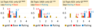
Figure 8. Review count distributions at rank $k=10$ achieved by Base and Rating for three example topics, with the common gold distribution.

Table 5. DistrSim and revcnt-GF scores for the cases shown in Figure 8. Higher (i.e., better) scores are shown in bold.

	DistrSim / GF (JSD)	DistrSim / GF (NMD)	DistrSim / GF (RNOD)
(a) Topic 416 (GFNMD is the outlier)
Base	0.801 / 0.572	0.742 / 0.566	0.712 / 0.505
Rating	0.730 / 0.366	0.807 / 0.576	0.668 / 0.365
(b) Topic 1469 (GFJSD is the outlier)
Base	0.765 / 0.554	0.708 / 0.553	0.643 / 0.480
Rating	0.801 / 0.532	0.742 / 0.614	0.712 / 0.512
(c) Topic 823 (GFRNOD is the outlier)
Base	0.574 / 0.417	0.458 / 0.454	0.464 / 0.380
Rating	0.521 / 0.408	0.492 / 0.423)	0.528 / 0.414

To investigate the differences in the DistrSim functions and the revcnt-GF measures that are based on them, we first filtered the 418 queries and obtained those where one of the three GF measures disagreed with the other two; there were 102 such queries. Within this query set, revcnt-GF^NMD disagreed with the other two for 83 queries (Case A); revcnt-GF^JSD disagreed with the other two for 16 queries (Case B); and revcnt-GF^RNOD disagreed with the other two for the remaining 3 queries (Case C). These results also show that revcnt-GF^NMD tends to be the outlier. It is known that RNOD lies between JSD and NMD in terms of how it behaves as a divergence measure (Sakai, 2020, 2021a): our results show that the GF measures inherit their properties, as the GF measures are essentially weighted averages of DistrSim scores obtained at each rank (See Eq. 7).

To examine how these discrepancies between the three revcnt-GF measures arise, we selected one topic each from Cases A, B, and C with relatively large score discrepancies, and examined the results closely. Figure 8 visualises the distributions over the review count groups achieved at rank 10 by Base and Rating for the three selected topics, together with the common gold distribution. Table 5 shows the corresponding DistrSim scores as well as the final revcnt-GF scores. Table 5(a) shows that for Topic 416, GF^NMD disagrees with GF^JSD and GF^RNOD precisely because $\textit{DistrSim}^{\mathrm{NMD}}$ disagrees with $\textit{DistrSim}^{\mathrm{JSD}}$ and $\textit{DistrSim}^{\mathrm{RNOD}}$. However, Figure 8(a) shows that this behaviour of $\textit{DistrSim}^{\mathrm{NMD}}$ is rather counterintuitive: since the gold distribution gives the highest probability to the zero-review group (Group 1), the achieved distribution of Base (red) seems better than that of Rating (blue). On the other hand, Table 5(b) shows that for Topic 1469, while GF^JSD disagrees with the other two, all three DistrSim functions agree that Rating is better than Base at rank 10. (Figure 8(b) shows the distributions.) That is, this discrepancy at the GF score level is due to the RBP-based weighted averaging step of Eq. 7. Finally, Table 5(c) shows that for Topic 823, while GF^RNOD is the outlier at the GF score level, both $\textit{DistrSim}^{\mathrm{NMD}}$ and $\textit{DistrSim}^{\mathrm{RNOD}}$ (i.e., those that can handle ordinal classes) prefer Rating over Base. That is, $\textit{DistrSim}^{\mathrm{JSD}}$ is the actual outlier at the DistrSim level. From Figure 8(c), it can be observed that, for this topic, the order-aware measures penalise Base heavily for emphasing Group 4 (items with over 100 reviews) too much. Based on the above analysis, our recommendation for handling ordinal attribute sets is to use multiple similarity functions (e.g., $\textit{DistrSim}^{\mathrm{JSD}}$ and $\textit{DistrSim}^{\mathrm{RNOD}}$), pay attention to cases where they disagree, and, if possible, examine which function seems more intuitive. As we have discussed in Section 1, researchers should also be aware that JSD ignores the ordinal nature of classes and therefore may not be appropriate for some applications.

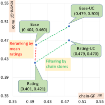
Figure 9. Visualising intersectional group fairness using GF measures for the local search runs.

Figure 9 provides a visual summary of our Local Search experiment, by plotting the revcnt-GF^RNOD scores against the chain-GF^JSD scores for the 4 runs we considered. Again, it is clear that the Unique Chain filtering step improves the ranking in terms of both chain-based and revcnt-based group fairness (green arrows), and that reranking by mean rating hurts the revcnt-based group fairness only (red arrow). We have thus demonstrated that our framework enables researchers to study intersectional group fairness, even when both nominal and ordinal attribute sets are involved.

We have also conducted a smaller experiment with both nominal and ordinal attribute sets using data available from Inside Airbnb (Biega et al., 2018). The results are similar to what we have reported here, and are omitted in this paper.

5. Conclusions

We presented a simple and versatile framework for evaluating ranked lists in terms of group fairness and relevance, where the groups can be either nominal or ordinal in nature. First, we demonstrated that, if the attribute set is binary, our framework can easily quantify the overall polarity of each ranked list. Second, by utilising an existing diversified search test collection and treating each intent as an attribute value, we demonstrated that our framework can handle soft group membership, and that our group fairness measures are highly correlated with both adhoc IR and diversified IR measures under this setting. Third, we demonstrated how our framework can quantify intersectional group fairness based on multiple attribute sets. We also showed that the choice of the similarity function for comparing the achieved and target distributions over the attribute values matters in some cases. Our recommendation is to use multiple similarity functions (e.g., $\textit{DistrSim}^{\mathrm{JSD}}$ and $\textit{DistrSim}^{\mathrm{RNOD}}$) if ordinal attribute values need to be considered. Data that are necessary for reproducing our experimental results are available from https://waseda.box.com/GFR20220401targz .

Our future work includes further investigation of the properties of the similarity functions in the context of group-fair ranking evaluation, and implementing this framework in a shared task.

References

- (1)
- Agrawal et al. (2009) Rakesh Agrawal, Gollapudi Sreenivas, Alan Halverson, and Samuel Leong. 2009. Diversifying Search Results. In Proceedings of ACM WSDM 2009. 5–14.
- Ajjour et al. (2019) Yamen Ajjour, Henning Wachsmuth, Johannes Kiesel, Martin Potthast, Matthias Hagen, and Benno Stein. 2019. Data Acquisition for Argument Search: The args.me Corpus. In KI 2019: Advances in Artificial Intelligence (LNCS 11793). 48–59.
- Amigó et al. (2018) Enrique Amigó, Damiano Spina, and Jorge Carrillo de Albornoz. 2018. An Axiomatic Analysis of Diversity Evaluation Metrics: Introducting the Rank-Biased Utility Metric. In Proceedings of ACM SIGIR 2018. 625–634.
- Beutel et al. (2019) Alex Beutel, Jilin Chen, Tulsee Doshi, Hai Qian, Li Wei, Yi Wu, Lukasz Heldt, Zhe Zhao, Lichan Hong, Ed H. Chi, and Cristos Goodrow. 2019. Fairness in Recommendation Ranking through Pairwise Comparisons. In Proceedings of ACM KDD 2019. 2212–2220.
- Biega et al. (2021) Asia J Biega, Fernando Diaz, Michael D. Ekstrand, Sergey Feldman, and Sebastian Kohlmeier. 2021. Overview of the TREC 2020 Fair Ranking Track. In Proceedings of TREC 2020.
- Biega et al. (2020) Asia J Biega, Fernando Diaz, Michael D. Ekstrand, and Sebastian Kohlmeier. 2020. Overview of the TREC 2019 Fair Ranking Track. In Proceedings of TREC 2019.
- Biega et al. (2018) Asia J. Biega, Krishna P. Gummadi, and Gerhard Weikum. 2018. Equity of Attention: Amortizing Individual Fairness in Rankings. In Proceedings of ACM SIGIR 2018. 405–414.
- Bondarenko et al. (2020) Alexander Bondarenko, Maik Fröbe, Meriem Beloucif, Lukas Gienapp, Yamen Ajjour, Alexander Panchenko, Chris Biemann, Benno Stein, Henning Wachsmuth, Martin Potthast, and Matthias Hagen. 2020. Overview of Touché 2020: Argument Retrieval. In Proceedings of CLEF 2020 (LNCS 12260). 384–395.
- Bondarenko et al. (2021) Alexander Bondarenko, Lukas Gienapp, Maik Fröbe, Meriem Beloucif, Yamen Ajjour, , Alexander Panchenko, Chris Biemann, Benno Stein, Henning Wachsmuth, Martin Potthast, and Matthias Hagen. 2021. Overview of Touché 2020: Argument Retrieval. In Proceedings of CLEF 2021 (LNCS 12880). 450–467.
- Buolamwini and Gebru (2018) Joy Buolamwini and Timnit Gebru. 2018. Gender Shades: Intersectional Accuracy Disparities in Commercial Gender Classification. In Proceedings of Machine Learning Research, Vol. 81. 77–91.
- Celis et al. (2017) L. Elisa Celis, Damian Straszak, and Nisheeth K. Vishnoi. 2017. Ranking with Fairness Constraints. (2017). http://arxiv.org/abs/1704.06840
- Chapelle et al. (2011) Olivier Chapelle, Shihao Ji, Ciya Liao, Emre Velipasaoglu, Larry Lai, and Su-Lin Wu. 2011. Intent-based Diversification of Web Search Results: Metrics and Algorithms. Information Retrieval 14, 6 (2011), 572–592.
- Chapelle et al. (2009) Olivier Chapelle, Donald Metzler, Ya Zhang, and Pierre Grinspan. 2009. Expected Reciprocal Rank for Graded Relevance. In Proceedings of ACM CIKM 2009. 621–630.
- Cherumanal et al. (2021) Sachin Pathiyan Cherumanal, Damiano Spina, Falk Scholer, and W. Bruce Croft. 2021. Evaluating Fairness in Argument Retrieval. In Proceedings of ACM CIKM 2021.
- Clarke et al. (2011) Charles L.A. Clarke, Nick Craswell, Ian Soboroff, and Azin Ashkan. 2011. A Comparative Analysis of Cascade Measures for Novelty and Diversity. In Proceedings of ACM WSDM 2011. 75–84.
- Clarke et al. (2013) Charles L.A. Clarke, Nick Craswell, and Ellen M. Voorhees. 2013. Overview of the TREC 2012 Web Track. In Proceedings of TREC 2012.
- Diaz et al. (2020) Fernando Diaz, Bhaskar Mitra, Michael D. Ekstrand, Asia J. Biega, and Ben Carterette. 2020. Evaluating Stochastic Rankings with Expected Exposure. In Proceedings of ACM CIKM 2020. 275–284.
- Draws et al. (2021) Tim Draws, Nava Tintarev, and Ujwal Gadiraju. 2021. Assessing Viewpoint Diversity in Search Results Using Ranking Fairness Metrics. ACM SIGKDD Explorations NewsLetter 23 (2021), 50–58. Issue 1.
- Ekstrand et al. (2021) Michael D. Ekstrand, Anubrata Das, Robin Burke, and Fernando Diaz. 2021. Fairness and Discrimination in Information Access Systems. (2021). https://arxiv.org/abs/2105.05779
- Foulds et al. (2019) James R. Foulds, Rashidul Islam, Kamrun Naher Keya, and Shimei Pan. 2019. An Intersectional Definition of Fairness. CoRR abs/1807.08362 (2019). http://arxiv.org/abs/1807.08362
- Geyik et al. (2019) Sahin Cem Geyik, Stuart Ambler, and Krishnaram Kenthapadi. 2019. Fairness-aware Ranking in Search & Recommendation Systems with Application to LinkedIn Talent Search. In Proceedings of ACK KDD 2019. 2221–2231.
- Gezici et al. (2021) Gizem Gezici, Aldo Lipani, Yucel Saygin, and Emine Yilmaz. 2021. Evaluation Metrics for Measuring Bias in Search Engine Results. Information Retrieval Journal 24 (2021), 85–113.
- Ghosh et al. (2021a) Avijit Ghosh, Ritam Dutt, and Christo Wilson. 2021a. When Fair Ranking Meets Uncertain Inference. In Proceedings of ACM SIGIR 2021. 1033–1043.
- Ghosh et al. (2021b) Avijit Ghosh, Lea Genuit, and Mary Reagan. 2021b. Characterizing Intersectional Group Fairness with Worst-Case Comparisons. CoRR abs/2101.01673 (2021). https://arxiv.org/abs/2101.01673
- Järvelin and Kekäläinen (2002) Kalervo Järvelin and Jaana Kekäläinen. 2002. Cumulated Gain-based Evaluation of IR Techniques. ACM TOIS 20, 4 (2002), 422–446.
- Kuhlman et al. (2021) Caitlin Kuhlman, Walter Gerych, and Elke Rundensteiner. 2021. Measuring Group Advantage: A Comparative Study of Fair Ranking Metrics. In Proceedings of AAAI/ACM AIES 2021. 674–682.
- Kuhlman et al. (2019) Caitlin Kuhlman, MaryAnn VanValkenburg, and Elke Rundensteiner. 2019. FARE: Diagnostics for Fair Ranking using Pairwise Error Metrics. In Proceedings of WWW 2019. 2936–2942.
- Kulshrestha et al. (2017) Juhi Kulshrestha, Motahhare Eslami, Johnnatan Messias, Muhammad Bilal Zafar, Saptarshi Ghosh, Krishna P. Gunmadi, and Karrie Karahalios. 2017. Quantifying Search Bias: Investigating Sources of Bias for Political Searches in Social Media. In Proceedings of ACM CSCW 2017. 417–432.
- Lin (1991) Jianhua Lin. 1991. Divergence Measures Based on the Shannon Entropy. IEEE Transactions on Information Theory 37, 1 (1991), 145–151.
- Moffat et al. (2017) Alistair Moffat, Peter Bailey, Falk Scholer, and Paul Thomas. 2017. Incorporating User Expectations and Behavior into the Measurement of Search Effectiveness. ACM TOIS 35, 3 (2017).
- Moffat and Zobel (2008) Alistair Moffat and Justin Zobel. 2008. Rank-Biased Precision for Measurement of Retrieval Effectiveness. ACM TOIS 27, 1 (2008).
- Narasimhan et al. (2020) Harikrishna Narasimhan, Andrew Cotter, Maya Gupta, and Serena Wang. 2020. Pairwise Fairness for Ranking and Regression. In Proceedings of AAAI 2020. 5248–5255.
- Ömer Kirnap et al. (2021) Ömer Kirnap, Fernando Diaz, Asia Biega, Michael Ekstrand, Ben Carterette, and Emine Yilmaz. 2021. Estimation of Fair Ranking Metrics with Incomplete Judgments. In Proceedings of WWW 2021. 1065–1075.
- Pitoura et al. (2017) Evaggelia Pitoura, Panayiotis Tsaparas, Giorgos Flouris, Irini Fundulaki, Panagiotis Papadakos, Serge Abiteboul, and Gerhard Weikum. 2017. On Measuring Bias in Online Information. ACM SIGMOD Record 46 (2017), 16–21. Issue 4.
- Raj et al. (2020) Amifa Raj, Connor Wood, Ananda Montoly, and Michael D. Ekstrand. 2020. Comparing Fair Ranking Metrics. (2020). https://arxiv.org/abs/2009.01311
- Robertson et al. (2018) Ronald E. Robertson, Shan Jiang, Kenneth Joseph, Lisa Friedland, David Lazer, and Christo Wilson. 2018. Auditing Partisan Audience Bias within Google Search. In Proceedings of the ACM on Human-Computer Interaction, Vol. 2.
- Sakai (2007) Tetsuya Sakai. 2007. Alternatives to Bpref. In Proceedings of ACM SIGIR 2007. 71–78.
- Sakai (2014) Tetsuya Sakai. 2014. Metrics, Statistics, Tests. In PROMISE Winter School 2013: Bridging between Information Retrieval and Databases (LNCS 8173). 116–163.
- Sakai (2018) Tetsuya Sakai. 2018. Laboratory Experiments in Information Retrieval: Sample Sizes, Effect Sizes, and Statistical Power. Springer.
- Sakai (2020) Tetsuya Sakai. 2020. Evaluating Evaluation Measures for Ordinal Classification and Ordinal Quantification. In Proceedings of ACL-IJCNLP 2021. 2759–2769.
- Sakai (2021a) Tetsuya Sakai. 2021a. A Closer Look at Evaluation Measures for Ordinal Quantification. In Proceedings of the 1st International Workshop on Learning to Quantify.
- Sakai (2021b) Tetsuya Sakai. 2021b. On the Instability of Diminishing Return IR Measures. In Proceedings of ECIR 2021 Part I (LNCS 12656). 572–586.
- Sakai and Song (2011) Tetsuya Sakai and Ruihua Song. 2011. Evaluating Diversified Search Results using Per-intent Graded Relevance. In Proceedings of ACM SIGIR 2011. 1043–1052.
- Sakai and Zeng (2020) Tetsuya Sakai and Zhaohao Zeng. 2020. Retrieval Evaluation Measures that Agree with Users’ SERP Preferences: Traditional, Preference-based, and Diversity Measures. ACM TOIS 39, 2 (2020).
- Sapiezynski et al. (2019) Piotr Sapiezynski, Wesley Zeng, and Ronald E. Robertson. 2019. Quantifying the Impact of User Attention on Fair Group Representation in Ranked Lists. In Companion Proceedings of WWW 2019. 553–562.
- Singh and Joachims (2018) Ashudeep Singh and Thorsten Joachims. 2018. Fairness of Exposure in Rankings. In Proceedings of ACM KDD 2018. 2219–2228.
- Song et al. (2011) Ruihua Song, Min Zhang, Tetsuya Sakai, Makoto P. Kato, Yiqun Liu, Miho Sugimoto, Qinglei Wang, and Naoki Orii. 2011. Overview of the NTCIR-9 INTENT Task. In Proceedings of NTCIR-9. 82–105.
- Werman et al. (1985) Michael Werman, Shmuel Peleg, and Azriel Rosenfeld. 1985. A Distance Metric for Multidimensional Histograms. Computer Vision, Graphics, and Image Processing 32 (1985), 328–336.
- Yang and Stoyanovich (2017) Ke Yang and Julia Stoyanovich. 2017. Measuring Fairness in Ranked Outputs. In Proceedings of SSDBM 2017.
- Zehlike et al. (2017) Meike Zehlike, Francesco Bonchi, Carlos Castillo, Sara Hajian, Mohamed Megahed, and Ricardo Baeza-Yates. 2017. FA*IR: A Fair Top-k Ranking Algorithm. In Proceedings of ACM CIKM 2017. 1569–1578.
- Zhai et al. (2003) ChengXiang Zhai, William W. Cohen, and John Lafferty. 2003. Beyond Independent Relevance: Methods and Evaluation Metrics for Subtopic Retrieval. In Proceedings of ACM SIGIR 2003. 10–17.