Globally Optimal Spectrum- and Energy-Efficient Beamforming for Rate Splitting Multiple Access

Abstract

Rate splitting multiple access (RSMA) is a promising non-orthogonal transmission strategy for next-generation wireless networks. It has been shown to outperform existing multiple access schemes in terms of spectral and energy efficiency when suboptimal beamforming schemes are employed. In this work, we fill the gap between suboptimal and truly optimal beamforming schemes and conclusively establish the superior spectral and energy efficiency of RSMA. To this end, we propose a successive incumbent transcending (SIT) branch and bound (BB) algorithm to find globally optimal beamforming solutions that maximize the weighted sum rate or energy efficiency of RSMA in Gaussian multiple-input single-output (MISO) broadcast channels. Numerical results show that RSMA exhibits an explicit globally optimal spectral and energy efficiency gain over conventional multi-user linear precoding (MU-LP) and power-domain non-orthogonal multiple access (NOMA). Compared to existing globally optimal beamforming algorithms for MU-LP, the proposed SIT BB not only improves the numerical stability but also achieves faster convergence. Moreover, for the first time, we show that the spectral/energy efficiency of RSMA achieved by suboptimal beamforming schemes (including weighted minimum mean squared error (WMMSE) and successive convex approximation) almost coincides with the corresponding globally optimal performance, making it a valid choice for performance comparisons. The globally optimal results provided in this work are imperative to the ongoing research on RSMA as they serve as benchmarks for existing suboptimal beamforming strategies and those to be developed in multi-antenna broadcast channels.

I Introduction

Over the past few years, rate splitting multiple access (RSMA) , built upon the concept of rate splitting (RS) , has emerged as a promising non-orthogonal physical (PHY) -layer transmission paradigm for interference management and multiple access in modern multi-antenna communication networks [2, 3, 4]. The key design principle of RSMA is to partially decode the multi-user interference and partially treat it as noise. This is done by splitting user messages into common and private parts, respectively, and then transmitting them employing superposition coding [5]. The common message is decoded by multiple users, while the private message is only decoded by the corresponding user employing successive interference cancellation (SIC) . By flexibly adjusting the message splits according to the interference level, RSMA allows arbitrary combinations of joint decoding and treating interference as noise. Therefore, RSMA is a powerful interference management and multiple access strategy that softly bridges and subsumes existing schemes such as space division multiple access (SDMA) , which fully treats interference as noise, non-orthogonal multiple access (NOMA) , which fully decodes interference, and orthogonal multiple access (OMA) , which completely avoids interference by allocating orthogonal radio resources among users [3, 6].

The concept of RS was introduced forty years ago for the two-user single-input single-output (SISO) interference channel (IC) [7, 8]. However, the use of RS as a building block of RSMA is motivated by the recent progress of RS -based network design in multi-antenna wireless networks: RS was first shown to achieve the optimal degrees of freedom (DoF) region of underloaded multiple-input single-output (MISO) broadcast channels (BCs) with partial channel state information at the transmitter (CSIT) in [9] and of overloaded MISO BCs with heterogeneous CSIT in [10]. The DoF benefits of RS subsequently motivated investigations of RSMA precoder design at finite signal-to-noise ratios (SNRs) [11, 3, 12, 13, 6, 14, 15, 16]. There are two general lines of research for RSMA resource allocation, namely, low-complexity beamforming design [17, 18, 19, 6, 20, 19, 21, 22, 23] and beamforming optimization [11, 3, 24, 10, 14, 16, 15, 20, 12, 25, 26, 27, 28, 29] mainly with respect to maximizing the spectral efficiency (SE) or energy efficiency (EE) . Low-complexity beamforming approaches such as using random beamforming (RBF) [17, 30, 18, 19], matched beamforming (MBF) [21, 31, 22, 19, 6, 20], or singular value decomposition (SVD) [11] for the common stream together with zero-forcing (ZF) [17, 30, 18] or reguralized-zero forcing beamforming (RZF)/minimum mean square error (MMSE) [21, 31, 22, 19] for the private streams have been widely studied in RSMA -aided MISO BC . Block diagonalization (BD) [23, 18] has been further investigated when the receivers are equipped with multiple antennas. Instead, precoder optimization strives to find optimal beamformers that maximize achievable performance regions of RSMA. Existing beamforming design algorithms such as weighted minimum mean squared error (WMMSE) [11, 3, 24, 10, 13], successive convex approximation (SCA) [14, 15, 13, 20, 12, 25, 16, 29, 32, 25], alternating direction method of multipliers (ADMM) [33, 26, 34], and semidefinite relaxation (SDR) [16, 27, 28, 29] have been investigated for RSMA. SCA -based algorithms follow the classical idea of successively approximating the original non-convex problem with a sequence of convex approximations. WMMSE and ADMM -based algorithms are the block-wise alternative optimization where the variables are divided into blocks and the original problem is optimized alternatively with respect to a single block of variables while the rest of the blocks are held fixed. All of them could only guarantee a locally optimal point of the original problem [35]. Though SDR has the potential to find the global optimum, existing works all focus on combining SDR with other efficient approaches such as SCA [16, 29], gradient-based approach [27], particle swarm optimization [28], heuristic approaches [36] in order to reduce the computational complexity. Therefore, the solutions obtained in these works cannot ensure global optimality. Table I summarizes the state-of-the-art beamforming design approaches that have been proposed for RSMA . None of them exhibits strong optimality guarantees. Hence, all performance analyses based on these approaches are incapable of conclusively establishing the superiority of RSMA over the previously mentioned multiplexing schemes. To the best of the authors knowledge, there is no existing work focusing on the globally optimal beamforming design of RSMA , and the maximum SE and EE performance achieved by RSMA remains unknown.

TABLE I: Survey of existing RSMA beamforming design approaches.

Beamforming approach		Maximize SE	Maximize EE
Low	RBF + ZF	[17, 30, 18]	—
complexity	RBF + RZF	[19]	—
	MBF + ZF	[6]	[20]
	MBF + RZF	[19, 21, 31, 22]	—
	SVD + ZF	[11]	—
	MBF + BD	[23]	—
Suboptimal	WMMSE-based	[11, 3, 24, 10, 13]	—
	SCA-based	[14, 15, 13, 20, 16, 29]	[12, 25, 32]
	ADMM-based	[33, 26, 34]	—
	SDR-based	[16, 29]	—
Globally	SIT BB	This work	This work
optimal

The goal of this paper is to bridge this gap and derive an algorithm to determine a globally optimal beamforming solution for RSMA with respect to weighted sum rate (WSR) and EE maximization. The corresponding optimization problem is related to joint multicast and unicast precoding that is known to be NP-hard [37, 38]. While several globally optimal algorithms for unicast beamforming [39, 40] and multicast beamforming [41] exist, joint solution methods are scarce. In particular, the procedure in [42] solves the power minimization problem and [43] maximizes the WSR for joint multicast and unicast beamforming. All these methods are based on branch and bound (BB) in combination with the second-order cone (SOC) transformation in [44]. However, as this transformation moves the complexity into the feasible set, pure BB methods are prone to numerical problems, see Section III. Instead, in this paper we design a successive incumbent transcending (SIT) BB algorithm to solve this beamforming problem with improved numerical stability and faster convergence. To the best of the authors knowledge, this is the first globally optimal solution algorithm for an instance of the joint unicast and multicast problem with respect to EE maximization.

To summarize, the contributions of this paper are:

1. We develop a numerical solver for the WSR and EE beamforming problem in RSMA with guaranteed convergence to a globally optimal solution. We emphasize the novelty of the globally optimal EE maximization method for an instance of the joint unicast and multicast beamforming problem.

2. We apply the successive incumbent transcending (SIT)principle to a MISO beamforming problem. The proposed algorithm incorporates multi-user linear precoding (MU-LP) and 2-user NOMA beamforming as special cases. It exhibits faster practical convergence and improved numerical stability over state-of-the-art solution methods for MU-LP beamforming.

3. From a theoretical perspective, we establish finite convergence to the optimal solution. This property does not hold for most BB -based beamforming algorithms.

4. Extensive numerical verification is done, both to assess the numerical properties of the proposed algorithm and to evaluate the performance of suboptimal state-of-the-art methods. In particular, we show that these methods, including WMMSE and SCA , are often close to the true optimum solution.

The paper organization continues as follows. In the next section, we define the system model, formally state the optimization problem and transform it into an equivalent form more suitable for numerical solution. In Section III, the mathematical fundamentals of the proposed algorithm are reviewed. These are applied in Section IV to derive the solution algorithm and prove its convergence. We close the paper with numerical experiments in Section V and a short discussion.

Notation

Scalars and functions are typeset in normal font $x$. The absolute value of $\cdot$ is $|\cdot|$ and $v(\text{n})$ is the optimal value of the optimization problem in equation (n). $\Re\{\cdot\}$ and $\Im\{\cdot\}$ are the real and imaginary parts of a complex number, $j$ is the imaginary unit, and $\angle\cdot$ is the argument of $(\cdot)$. A vector $\bm{x}$ has components $[x_{1},x_{2},\dots]^{T}$ and is a column vector unless noted otherwise. The all-zero and all-ones vectors are denoted as $\bm{0}$ and $\bm{1}$, respectively. The operators $(\cdot)^{T}$, $(\cdot)^{H}$, and $\|\cdot\|$ are the transpose, the conjugate transpose and the Euclidean norm, respectively. Scalar operators are applied element-wise to vectors, where relational operators evaluate to true if they hold element-wise for all elements. A set is written as $\mathcal{X}$ and a family of sets as $\mathscr{X}$. The sets of real and complex numbers are denoted as $\mathds{R}$ and $\mathds{C}$. The notation $\mathcal{X}\setminus x$ is a shorthand for $\mathcal{X}\setminus\{x\}$. Let $\mathcal{X}$ and $(\bm{x},\bm{y})\in\mathcal{X}$. Then, $\operatorname{proj}_{\bm{x}}\mathcal{X}=\{\bm{x}:(\bm{x},\bm{y})\in\mathcal{X}\ \text{for some}\ \bm{y}\}$, i.e., the projection of $\mathcal{A}$ onto the $\bm{x}$ coordinates.

II System Model & Problem Statement

Consider the downlink in a wireless network where an $M$ antenna base station (BS) serves $K$ single-antenna users. The received signal at user $k$, $k\in\mathcal{K}=\{1,\dots,K\}$, for each channel use is $y_{k}=\bm{h}_{k}^{H}\bm{x}+n_{k}$, where the transmit signal $\bm{x}\in\mathds{C}^{M\times 1}$ is subject to an average power constraint $P$, $\bm{h}_{k}$ is the complex-valued channel from the BS to user $k$, and $n_{k}$ is circularly symmetric complex white Gaussian noise with unit power at user $k$. We assume perfect channel state information (CSI) at the transmitter and receivers.

The transmitter employs 1-layer RS [3, 11] as illustrated in Fig. 1, i.e., it splits the message $W_{k}$ intended for user $k$ into a common part $W_{c,k}$ and a private part $W_{p,k}$. Then, the common messages $W_{c,1},\ldots,W_{c,K}$ are combined into a single message $W_{c}$ and the $K+1$ resulting messages are encoded into independent Gaussian data streams $s_{c},s_{1},\dots,s_{K}$, each having unit power. These symbols are combined with linear precoding into the transmit signal $\bm{x}=\bm{p}_{c}s_{c}+\sum_{k\in\mathcal{K}}\bm{p}_{k}s_{k}$, where $\bm{p}_{c},\bm{p}_{1},\dots,\bm{p}_{K}\in\mathds{C}^{M}$ are the precoding vectors. Due to the average transmit power constraint, they need to satisfy $\|\bm{p}_{c}\|^{2}+\sum_{k\in\mathcal{K}}\|\bm{p}_{k}\|^{2}\leq P$.

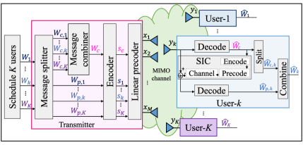
Figure 1: 1-layer RS model for $K$ users, where the common stream $s_{c}$ is shared by all users.

Each receiver $k\in\mathcal{K}$ uses SIC to first recover $s_{c}$ and then $s_{k}$ from its received signal $y_{k}$. In particular, $s_{c}$ is decoded first by treating interference from all other streams as noise. This allows user $k$ to recover its desired common part $W_{c,k}$. Then, $s_{c}$ is cancelled from the received signal and user $k$ proceeds to decode $s_{k}$ to recover the desired private part $W_{p,k}$. These two messages are combined to obtain $W_{k}$.

Given a precoding scheme $\bm{p}_{c},\bm{p}_{1},\dots,\bm{p}_{K}$, asymptotic error free decoding of $W_{c}$ and $W_{p,k}$ is possible if the rates of these messages satisfy

$$R_{c} \leq\log(1+\gamma_{c,k}),\forall k\in\mathcal{K}, R_{p,k} \leq\log(1+\gamma_{p,k})$$ (1)

with signal to interference plus noise ratios (SINRs)

$$\gamma_{c,k} =\frac{|{\bm{h}}_{k}^{H}\bm{p}_{c}|^{2}}{\sum\limits_{j\in\mathcal{K}}|\bm{h}_{k}^{H}\bm{p}_{j}|^{2}+1}, \gamma_{p,k} =\frac{|{\bm{h}}_{k}^{H}\bm{p}_{k}|^{2}}{\sum\limits_{j\in\mathcal{K}\setminus k}|\bm{h}_{k}^{H}\bm{p}_{j}|^{2}+1}.$$ (2)

The rate $R_{c}$ is shared across the users, where user $k$ is allocated a portion ${C}_{k}$ corresponding to the rate of $W_{c,k}$, such that $\sum_{k\in\mathcal{K}}{C}_{k}={R}_{c}$. The total rate of user $k$ is $R_{k}=C_{k}+R_{p,k}$.

Observe that this system model can be interpreted as an instance of the joint multicast and unicast beamforming problem. It includes several notable special cases. With $\bm{p}_{c}=0$, we obtain MU-LP and for $\bm{p}_{k}=0$, $k\in\mathcal{K}$, it is the multicast beamforming problem. It also includes 2-user NOMA [6].

II-A Problem Statement

We consider WSR maximization under minimum rate Quality of Service (QoS) constraints, i.e.,

$$\max_{\begin{subarray}{c}\bm{p}_{1},\dots,\bm{p}_{K},\bm{p}_{c},\\ \bm{C},\bm{R}_{c},\bm{R}_{p},\bm{\gamma}_{c},\bm{\gamma}_{p}\end{subarray}}\quad \sum_{k\in\mathcal{K}}u_{k}\left(C_{k}+R_{p,k}\right)$$ (3a)

s.t. $$R_{c},R_{p,k},\gamma_{c,k}\text{ and }\gamma_{p,k}\text{ as in \eqref{eq: instantanesous}--\eqref{eq: SINR cp}}$$ (3b)

$$\sum_{k^{\prime}\in\mathcal{K}}C_{k^{\prime}}\leq R_{c}$$ (3c)

$$C_{k}\geq 0,\enskip k\in\mathcal{K}$$ (3d)

$$C_{k}+R_{p,k}\geq R_{k}^{th},\enskip k\in\mathcal{K}$$ (3e)

$$\|\bm{p}_{c}\|^{2}+\sum_{k\in\mathcal{K}}\|\bm{p}_{k}\|^{2}\leq P$$ (3f)

with nonnegative weight vector $\bm{u}=[u_{1},\ldots,u_{K}]^{T}\neq\bm{0}$, where 3b includes the rate constraints and SINR definition from the system model, 3b ensures that the common rate allocations $C_{k}$ are feasible, 3c implements the non-negativity of the common rates, 3e is the minimum rate constraint with threshold $R_{k}^{th}$ for user $k$, and 3f is the maximum power constraint at the BS . We also consider EE maximization

$$\max_{\begin{subarray}{c}\bm{p}_{1},\dots,\bm{p}_{K},\bm{p}_{c},\\ \bm{C},R_{c},\bm{R}_{p},\bm{\gamma}_{c},\bm{\gamma}_{p}\end{subarray}}\quad \frac{\sum_{k\in\mathcal{K}}C_{k}+R_{p,k}}{\mu\left(\|\bm{p}_{c}\|^{2}+\sum_{k\in\mathcal{K}}\|\bm{p}_{k}\|^{2}\right)+P_{c}}$$ (4a)

s.t. $$\text{\lx@cref{creftypeplural~refnum}{eq:WSR QoS prob:2}, \lx@cref{refnum}{eq:WSR QoS prob:3}, \lx@cref{refnum}{eq:WSR QoS prob:4}, \lx@cref{refnum}{eq:WSR QoS prob:5} and~\lx@cref{refnum}{eq:WSR QoS prob:6}},$$ (4b)

where $\mu\geq 0$ is the power amplifier inefficiency and $P_{c}>0$ is the static circuit power consumption. For notational simplicity, we define $\bm{C}=[C_{1},\dots,C_{k}]^{T}$, $\bm{\gamma}_{p}=[\gamma_{1},\dots,\gamma_{K}]^{T}$, $\bm{\gamma}_{c}=[\gamma_{c,1},\dots,\gamma_{c,K}]^{T}$, $\bm{R}_{p}=[R_{p,1},\dots,R_{p,K}]^{T}$. Both problems can be combined into the equivalent optimization problem

$$\max_{\begin{subarray}{c}\bm{p}_{1},\dots,\bm{p}_{K},\\ \bm{p}_{c},\bm{C},\bm{\gamma}_{c},\bm{\gamma}_{p}\end{subarray}}\quad \frac{\sum_{k\in\mathcal{K}}u_{k}\left(C_{k}+\log(1+\gamma_{p,k})\right)}{\mu\left(\|\bm{p}_{c}\|^{2}+\sum_{k\in\mathcal{K}}\|\bm{p}_{k}\|^{2}\right)+P_{c}}$$ (5a)

s.t. $$\gamma_{c,k}\text{ and }\gamma_{p,k}\text{ as in \eqref{eq: SINR cp}}$$ (5b)

$$\sum_{k^{\prime}\in\mathcal{K}}C_{k^{\prime}}\leq\log(1+\gamma_{c,k}),\enskip k\in\mathcal{K}$$ (5c)

$$C_{k}\geq\max\!\left\{0,R_{k}^{th}\!-\log(1+\gamma_{p,k})\right\}\!,k\in\mathcal{K}$$ (5d)

$$\|\bm{p}_{c}\|^{2}+\sum_{k\in\mathcal{K}}\|\bm{p}_{k}\|^{2}\leq P,$$ (5e)

where 5d combines 3d and 3e into a single constraint. Clearly, we obtain WSR maximization for $\mu=0,P_{c}=1$ and EE maximization for $\bm{u}=\bm{1}$.

A globally optimal solution of 5 can be obtained by solving

$$\max_{\begin{subarray}{c}\bm{p}_{c},\bm{p}_{1},\dots,\bm{p}_{K},\\ \bm{C},\bm{\gamma}_{p},s,\bm{d},\bm{e}\end{subarray}}{} \frac{\sum_{k\in\mathcal{K}}u_{k}\left(C_{k}+\log(1+\gamma_{p,k})\right)}{\mu\left(\|\bm{p}_{c}\|^{2}+\sum_{k\in\mathcal{K}}\|\bm{p}_{k}\|^{2}\right)+P_{c}}$$ (6a)

s.t. $$\sqrt{\gamma_{p,k}}\smash{\left(\sum\nolimits_{j\in\mathcal{K}\setminus k}|\bm{h}_{k}^{H}\bm{p}_{j}|^{2}+1\right)^{1/2}}\!\!\!\leq{\bm{h}}_{k}^{H}\bm{p}_{k}$$ (6b)

$$\sqrt{s}\left(\sum\nolimits_{j\in\mathcal{K}}|\bm{h}_{1}^{H}\bm{p}_{j}|^{2}+1\right)^{1/2}\leq{\bm{h}}_{1}^{H}\bm{p}_{c}$$ (6c)

$$\sqrt{s}\left(\sum\nolimits_{j\in\mathcal{K}}|\bm{h}_{k}^{H}\bm{p}_{j}|^{2}+1\right)^{1/2}\!\leq d_{k},\forall k>1$$ (6d)

$$(e_{k},d_{k})\in\mathcal{C},\forall k>1$$ (6e)

$$\Re\{\bm{h}_{k}^{H}\bm{p}_{k}\}\geq 0,\quad\Im\{\bm{h}_{k}^{H}\bm{p}_{k}\}=0$$ (6f)

$$\Re\{\bm{h}_{1}^{H}\bm{p}_{c}\}\geq 0,\quad\Im\{\bm{h}_{1}^{H}\bm{p}_{c}\}=0$$ (6g)

$$\forall k>1:d_{k}\geq 0,\enskip e_{k}={\bm{h}}_{k}^{H}\bm{p}_{c}$$ (6h)

$$\sum_{k\in\mathcal{K}}C_{k}\leq\log(1+s)$$ (6i)

$$\eqref{eq:srmaxequiv:4}\text{ and }\eqref{eq:srmaxequiv:6}$$ (6j)

with

$$(e,d)\in\mathcal{C}=\{e\in\mathds{C},d\in\mathds{R}:d\leq|e|\}$$ (7)

instead of 5. A crucial observation is that this problem is a second-order cone program (SOCP) for fixed $s$, $\bm{\gamma}_{p}$ except for constraint 6h. Hence, the nonconvexity of 5 is only due to the SINR expressions and not due to the beamforming vectors. We will exploit this partial convexity in the final algorithm to limit the numerical complexity.

The transformation from 5 to 6 relies on the observation that, for all other variables except the beamforming vectors fixed, the nonconvexity in 5 stemming from $\bm{p}_{k}$ is only due to the product $|\bm{h}_{k}^{H}\bm{p}_{k}|^{2}$. This can be seen from considering 8b below and multiplying it with the denominator of its right-hand side (RHS) . Then, for fixed $\gamma_{p,k}$, one almost obtains the SOC 6b, except for $|\bm{h}_{k}^{H}\bm{p}_{k}|^{2}$. Further observing that the solution of 6 is rotationally invariant in $\bm{p}_{k}$, one can select the solution that results in $|\bm{h}_{k}^{H}\bm{p}_{k}|$ being nonnegative and real valued. This is achieved by introducing constraint 6f [44].

Unfortunately, this transformation is not sufficient to eliminate $\bm{p}_{c}$ as a nonconvex variable. This is because there is not a single product $|\bm{h}_{k}^{H}\bm{p}_{c}|^{2}$ that needs to be made real but $K$, one for each user. Our approach is to first replace $\gamma_{c,1},\dots,\gamma_{c,K}$ by a single nonconvex variable $s=\min_{k}\gamma_{c,k}$ and then apply the same transformation as for the precoders $\bm{p}_{1},\dots,\bm{p}_{K}$ for only one of the products $|\bm{h}_{k}^{H}\bm{p}_{c}|^{2}$ (here for $k=1$). This results in the constraints 6c and 6g. The remaining $K-1$ “almost”-SOC -constraints are then addressed using the argument cuts approach from [41]. In particular, real valued auxiliary variables $d_{k}$ are introduced together with the relaxation that these must be within the circle $|\bm{h}_{k}^{H}\bm{p}_{c}|$. These considerations will be made rigorous in Proposition 1.

Another equivalent variant of 5 that is interesting in its own right is

$$\max_{\begin{subarray}{c}\bm{p}_{c},\bm{p}_{1},\dots,\bm{p}_{K},\\ \bm{C},\bm{\gamma}_{p},s\end{subarray}}\quad \frac{\sum_{k\in\mathcal{K}}u_{k}\left(C_{k}+\log(1+\gamma_{p,k})\right)}{\mu\left(\|\bm{p}_{c}\|^{2}+\sum_{k\in\mathcal{K}}\|\bm{p}_{k}\|^{2}\right)+P_{c}}$$ (8a)

s.t. $$\gamma_{p,k}\leq\frac{|{\bm{h}}_{k}^{H}\bm{p}_{k}|^{2}}{\sum_{j\in\mathcal{K}\setminus k}|\bm{h}_{k}^{H}\bm{p}_{j}|^{2}+1}$$ (8b)

$$s\leq\frac{|{\bm{h}}_{k}^{H}\bm{p}_{c}|^{2}}{\sum_{j\in\mathcal{K}}|\bm{h}_{k}^{H}\bm{p}_{j}|^{2}+1},\enskip k\in\mathcal{K}$$ (8c)

$$\eqref{eq:srmaxequiv:4},\eqref{eq:srmaxequiv:6}\text{ and }\eqref{eq:srmax:9}.$$ (8d)

This problem is obtained as a side product when showing the equivalence of 5 and 6, which is established next.

Proposition 1

Let $\bm{x}^{\star}=(\bm{p}_{c}^{\star},\bm{p}_{1}^{\star},\dots,\bm{p}_{K}^{\star},\bm{C}^{\star},\bm{\gamma}_{p}^{\star})$. A point $(\bm{x}^{\star},s^{\star})$ solves 8 if $(\bm{x}^{\star},\bm{\gamma}_{c}^{\star})$ solves 5 and $s^{\star}=\min_{k}\gamma_{c,k}^{\star}$. Conversely, the point $(\bm{x}^{\star},\bm{\gamma}_{c}^{\star})$ solves 5 if $(\bm{x}^{\star},s^{\star})$ solves 8 and $\gamma_{c,k}^{\star}=\frac{|{\bm{h}}_{k}^{H}\bm{p}_{c}^{\star}|^{2}}{\sum_{j\in\mathcal{K}}|\bm{h}_{k}^{H}\bm{p}_{j}^{\star}|^{2}+1}$ for all $k\in\mathcal{K}$. Moreover, if $(\bm{x}^{\star},s^{\star},\bm{d}^{\star},\bm{e}^{\star})$ solves 6, then $(\bm{x}^{\star},s^{\star})$ solves 8 and $(\bm{x}^{\star},\bm{\gamma}_{c}^{\star})$ solves 5, where $s^{\star}$ and $\bm{\gamma}_{c}^{\star}$ are as before.

Proof:

See Appendix A. ∎

Corollary 1

Problems 5, 6 and 8 have the same optimal value.

In the next section, we introduce some mathematical preliminaries before we develop a solution algorithm for 6 in Section IV.

III Mathematical Background

Problem 6 is an NP-hard nonconvex optimization problem. To see this, consider problem 8 for $\mu=0$, $u_{k}=1$, and fix all variables except $\bm{p}_{c}$, $\bm{C}$ and $s$. Then, it is equivalent to

$$\max_{\bm{p}_{c}}\min_{k}\{|\tilde{\bm{h}}_{k}^{H}\bm{p}_{c}|^{2}\}\quad\mathrm{s.\,t.}\quad\|\bm{p}_{c}\|^{2}\leq\tilde{P}.$$ (9)

This is known as multicast beamforming and shown to be NP-hard in [37]. Our solution approach for this part of the problem relies on the so-called “argument cuts” proposed in [41]. The introduction of the auxiliary variables $d_{k}$ and $e_{k}$ in 6 is motivated by this approach and collects most of the nonconvexity due to $\bm{p}_{c}$ in 6e. The idea is to add a box constraint on $\arg(e_{k})$ to $\mathcal{C}$ and then optimize over its convex envelope to obtain a bound on 6 suitable for a BB procedure.

The remaining nonconvexity in 6 stems from $\gamma_{p,k}$ and $s$ in 6b, 6c and 6d. Previous global optimization algorithms for such problems rely on BB procedures with SOCP bounding [39, 40, 42, 43]. However, this leads to an infinite algorithm where the convergence to the global optimal solution cannot be guaranteed in a finite number of iterations. This is because the difficulty in solving 6 is due to the feasible set, while BB works best if the nonconvexity is mostly due to the objective. Please refer to [46, 47, 48] for a detailed discussion of this topic. For the solution of 6, finite convergence can be obtained by adding a line search procedure to every iteration of the BB procedure that recovers a feasible point and requires the solution of several SOC feasibility problems [39, Alg. 3]. Hence, finite convergence in BB procedures comes at the cost of increased computational complexity. Moreover, the auxiliary SOCP that is solved in every iteration of the BB procedure is numerically challenging as the feasible set can become very small. This leads to numerical problems even with commercial state-of-the-art solvers like Mosek [49]. A computationally more tractable modification is proposed in [39, §2.2.2] that comes at the price of much harder feasible point acquisition in the BB procedure.

Instead, we design an algorithm based on the SIT scheme [50, 51, 47, 48] and combine it with a branch reduce and bound (BRB) procedure. The resulting algorithm is numerically stable, has proven finite convergence, solves EE maximization and is the first global optimization algorithm specifically designed for RSMA . Practically, it outperforms algorithms for similar problems as will be verified in Section V. To better illustrate the core principles of SIT , we first consider the following general optimization problem

$$\max_{(\bm{x},\bm{\xi})\in\mathcal{D}}\enskip f(\bm{x},\bm{\xi})\quad\mathrm{s.\,t.}\quad g_{i}(\bm{x},\bm{\xi})\leq 0,\enskip i=1,\dots,n$$ (10)

with continuous, real-valued functions $f,g_{1},\dots,g_{n}$ and nonempty feasible set. Further, assume that $f$ is concave, $g_{1},\dots,g_{n}$ are convex in $\bm{\xi}$ for fixed $\bm{x}$, and $\mathcal{D}$ is a closed convex set. Depending on the structure of $g_{1},\dots,g_{n}$ in $\bm{x}$ this problem might be quite hard to solve for BB methods [52, 47]. By exchanging the objective and constraints of 10, we obtain the so-called SIT dual

$$\min_{(\bm{x},\bm{\xi})\in\mathcal{D}}\enskip\max_{i}\{g_{i}(\bm{x},\bm{\xi})\}\quad\mathrm{s.\,t.}\quad f(\bm{x},\bm{\xi})\geq\delta.$$ (11)

Observe that the optimal value of 10 is greater than or equal to $\delta$ if the optimal value of 11 is less than or equal to zero. Conversely, if the optimal value of 11 is greater than zero, the optimal value of 10 is less than $\delta$. Hence, the optimal solution of 10 can be obtained by solving a sequence of 11 with increasing $\delta$. Since the feasible set of 11 is closed and convex, it can be solved much easier by BB than 10.

Obtaining the exact optimal solution to continuous real-valued optimization problems is often computationally infeasible, even for linear or convex problems. A widely employed practice is to accept any feasible point with objective value within a prescribed tolerance $\eta$ of the exact optimal value as a solution. That is, a point $(\bar{\bm{x}},\bar{\bm{\xi}})$ is called an $\eta$-optimal solution of 10 if, for all feasible points $(\bm{x},\bm{\xi})$,

$$f(\bar{\bm{x}},\bar{\bm{\xi}})\geq f(\bm{x},\bm{\xi})-\eta.$$ (12)

Likewise, the constraints in 10 can be hard to satisfy numerically. The most common approach is to relax them by $\varepsilon$. However, for nonconvex feasible sets this can lead to completely wrong solutions [50, 52, 47]. Instead, for the SIT scheme, the constraints are tightened by $\varepsilon$, i.e., the problem to be solved is

$$\max_{(\bm{x},\bm{\xi})\in\mathcal{D}}\enskip f(\bm{x},\bm{\xi})\quad\mathrm{s.\,t.}\quad g_{i}(\bm{x},\bm{\xi})\leq-\varepsilon,\enskip i=1,\dots,n$$ (13)

for some $\varepsilon>0$. Any point in this feasible set is denoted as $\varepsilon$-essential feasible and a solution of this problem satisfying 12 is called essential $(\varepsilon,\eta)$-optimal solution of 10. This constraint tightening removes numerically instable points from the feasible set and is necessary to ensure finite convergence of the SIT scheme.

The outlined duality between 10 and 11 is formalized in the following lemma.

Lemma 1

For every $\varepsilon>0$, the $\varepsilon$-essential optimal value of 10 is less than $\delta$ if and only of the optimal value of 11 is greater than or equal to $-\varepsilon$.

Proof:

Direct consequence of [50, Prop. 1]. ∎

We refer to 10 as the primal problem and 11 as the dual problem.

III-A Successive Incumbent Transcending Algorithm

The discussion above leads to the SIT algorithm as stated in Algorithm 1. The core problem is Step 1, which is implemented by solving 11 with a modified rectangular BB procedure. Such a procedure has exponential computational complexity in the number of optimization variables. Since 11 is a convex optimization problem for fixed $\bm{x}$, the SIT BB procedure should only operate on the nonconvex variables $\bm{x}$ and employ a convex solver for $\bm{\xi}$ to limit the computational complexity.

Algorithm 1 SIT Algorithm [52, §7.5.1].

1. Initialize $(\bar{\bm{x}},\bar{\bm{\xi}})$ with the best known nonisolated feasible solution and set $\delta=f(\bar{\bm{x}},\bar{\bm{\xi}})+\eta$; otherwise do not set $(\bar{\bm{x}},\bar{\bm{\xi}})$ and choose $\delta\leq f(\bm{x},\bm{\xi})$ $\forall(\bm{x},\bm{\xi})\in\mathcal{D}$.

2. Check if 10 has a nonisolated feasible solution $(\bm{x},\bm{\xi})$ satisfying $f(\bm{x},\bm{\xi})\geq\delta$; otherwise, establish that no such $\varepsilon$-essential feasible $(\bm{x},\bm{\xi})$ exists and go to Step 3.

3. Update $(\bar{\bm{x}},\bar{\bm{\xi}})\leftarrow(\bm{x},\bm{\xi})$ and $\delta\leftarrow f(\bar{\bm{x}},\bar{\bm{\xi}})+\eta$. Go to Step 1.

4. Terminate: If $(\bar{\bm{x}},\bar{\bm{\xi}})$ is set, it is an essential $(\varepsilon,\eta)$-optimal solution; else Problem (10) is $\varepsilon$-essential infeasible.

The general idea of BB is to relax the feasible set and then subsequently partition this relaxed set in such a way that upper and lower bounds on the objective value in each partition can be computed efficiently. As the partition is successively refined, these bounds approach each other until the optimal value is found. For a rectangular BB procedure, the feasible set is relaxed into an initial box

$$\mathcal{M}_{0}=[\bm{r}^{0},\bm{s}^{0}]=\{\bm{x}:r^{0}_{i}\leq x_{i}\leq s^{0}_{i}\}$$ (14)

satisfying $\mathcal{M}_{0}\supseteq\operatorname{proj}_{\bm{x}}\mathcal{D}$. Further, a bounding function $\beta(\mathcal{M})$, $\mathcal{M}\subseteq\mathcal{M}_{0}$, with $\beta(\mathcal{M})=\infty$ if $\operatorname{proj}_{\bm{x}}\mathcal{F}\cap\mathcal{M}=\emptyset$ and

$$\beta(\mathcal{M})\leq\min_{\begin{subarray}{c}(\bm{x},\bm{\xi})\in\mathcal{F},\bm{x}\in\mathcal{M}\end{subarray}}\max_{i}\{g_{i}(\bm{x},\bm{\xi})\},$$ (15)

otherwise is required, where $\mathcal{F}=\{(\bm{x},\bm{\xi})\in\mathcal{D}:f(\bm{x},\bm{\xi})\geq\delta\}$ is the feasible set of 11. The algorithm subsequently partitions the relaxed feasible set $\mathcal{M}_{0}$ into smaller boxes and stores the current partition of $\mathcal{M}_{0}$ in a set $\mathscr{R}_{k}$. In iteration $k$, the algorithm uses best-first selection to determine the next branch, i.e.,

$$\mathcal{M}_{k}\in\operatorname*{arg\,min}\{\beta(\mathcal{M})\,|\,\mathcal{M}\in\mathscr{R}_{k}\},$$ (16)

and then replaces $\mathcal{M}_{k}=[\bm{r}^{k},\bm{s}^{k}]$ by two new subrectangles

$$\mathcal{M}^{-} =\{\bm{x}:r_{j}\leq x_{j}\leq v_{j},\ r_{i}\leq x_{i}\leq s_{i}\ (i\neq j)\}$$ (17a)

$$\mathcal{M}^{+} =\{\bm{x}:v_{j}\leq x_{j}\leq s_{j},\ r_{i}\leq x_{i}\leq s_{i}\ (i\neq j)\}$$ (17b)

with $\bm{v}=\frac{1}{2}(\bm{s}+\bm{r})$ and $j\in\operatorname*{arg\,max}_{j}s_{j}-r_{j}$. For each of these new boxes, a lower bound on the objective value is computed using the bounding function $\beta(\mathcal{M})$. To ensure convergence, the bounding needs to be consistent with branching, i.e., $\beta(\mathcal{M})$ has to satisfy

$$\beta(\mathcal{M})-\min_{\begin{subarray}{c}(\bm{x},\bm{\xi})\in\mathcal{F},\\ \bm{x}\in\mathcal{M}\end{subarray}}\max_{i}\{g_{i}(\bm{x},\bm{\xi})\}\rightarrow 0\enskip\mathrm{as}\enskip\max_{\bm{x},\bm{y}\in\mathcal{M}}\|\bm{x}-\bm{y}\|\rightarrow 0,$$ (18)

and a dual feasible point $\bm{x}^{k}\in\operatorname{proj}_{\bm{x}}\mathcal{F}\cap\mathcal{M}_{k}$ is required if $\beta(\mathcal{M}_{k})<\infty$. Suitable pruning and termination rules that ensure convergence can be obtained from the following lemma that is adapted from [52, Prop. 7.14] and [48, Prop. 5.9].

Lemma 2

Let $\varepsilon>0$ be given and define $g(\bm{x},\bm{\xi})=\max_{i}\{g_{i}(\bm{x},\bm{\xi})\}$. Let $\beta(\mathcal{M})$ satisfy 15 and 18 and $\mathcal{M}_{k}$ be as in 16. Then, as $\max_{\bm{x},\bm{y}\in\mathcal{M}_{k}}\|\bm{x}-\bm{y}\|\rightarrow 0$ for $k\to\infty$, either $g(\bm{x}^{k},\bm{\xi}^{*})<0$ for some $k$ and $(\bm{x}^{k},\bm{\xi}^{*})\in\mathcal{F}$ or $\beta(\mathcal{M}_{k})>-\varepsilon$ for some $k$. In the former case, $(\bm{x}^{k},\bm{\xi}^{*})$ is a nonisolated feasible solution of 10 satisfying $f(\bm{x}^{k},\bm{\xi}^{*})\geq\delta$. In the latter case, no $\varepsilon$-essential feasible solution $(\bm{x},\bm{\xi})$ of 10 exists such that $f(\bm{x},\bm{\xi})\geq\delta$.

Proof:

Please refer to [48, Prop. 5.9]. ∎

This suggests a BB procedure with pruning criterion $\beta(\mathcal{M})<-\varepsilon$ and termination criterion

$$0>\min\nolimits_{\bm{\xi}}\;g(\bm{x}^{k},\bm{\xi})\enskip\mathrm{s.\,t.}\enskip(\bm{x}^{k},\bm{\xi})\in\mathcal{F}.$$ (19)

In the following section, we apply this approach to find the solution of 6 and explicitly incorporate the outlined BB procedure into Algorithm 1.

IV Globally Optimal Beamforming

We design a globally optimal solution algorithm for 6 based on the fundamentals in the previous section. There, we have seen that the SIT algorithm requires a bounding function, a feasible point in each iteration and an initial box $\mathcal{M}_{0}$. These aspects will be discussed after identifying and discussing the SIT dual. At the end of this section, we state the complete algorithm and establish its convergence. We also derive a reduction procedure in Section IV-D that is essential for practical convergence, although it is not strictly necessary from a theoretical perspective.

The SIT dual should contain all of the problem’s nonconvexity in the objective function. Following the discussion in Section II-A, the nonconvexity in 6 is due to 6b, 6c, 6d and 6e and we obtain the SIT dual as

$$\min_{\begin{subarray}{c}\bm{p}_{c},\bm{p}_{1},\dots,\bm{p}_{K},\\ \bm{C},\bm{\gamma}_{p},s,\bm{d},\bm{e}\end{subarray}} \max\bigg{[}\sqrt{s}\left(\sum\nolimits_{j\in\mathcal{K}}|\bm{h}_{1}^{H}\bm{p}_{j}|^{2}+1\right)^{1/2}-{\bm{h}}_{1}^{H}\bm{p}_{c},$$

$$\quad\max_{k>1}\bigg{\{}\sqrt{s}\left(\sum\nolimits_{j\in\mathcal{K}}|\bm{h}_{k}^{H}\bm{p}_{j}|^{2}+1\right)^{1/2}\!\!\!\!\!-d_{k}\bigg{\}},$$

$$\max_{k\in\mathcal{K}}\bigg{\{}\sqrt{\gamma_{p,k}}\left(\sum\nolimits_{j\in\mathcal{K}\setminus k}|\bm{h}_{k}^{H}\bm{p}_{j}|^{2}+1\right)^{1/2}\!\!\!\!\!-{\bm{h}}_{k}^{H}\bm{p}_{k}\bigg{\}},$$

$$\quad\max_{k>1}\big{\{}d_{k}-|e_{k}|\big{\}}\bigg{]}$$ (20a)

s.t. $$\frac{\sum_{k\in\mathcal{K}}u_{k}\left(C_{k}+\log(1+\gamma_{p,k})\right)}{\mu\left(\|\bm{p}_{c}\|^{2}+\sum_{k\in\mathcal{K}}\|\bm{p}_{k}\|^{2}\right)+P_{c}}\geq\delta$$ (20b)

$$\text{\lx@cref{creftypeplural~refnum}{eq:srmax:4}, \lx@cref{refnum}{eq:srmax:5}, \lx@cref{refnum}{eq:srmax:7}, \lx@cref{refnum}{eq:srmax:9}, \lx@cref{refnum}{eq:srmaxequiv:4} and~\lx@cref{refnum}{eq:srmaxequiv:6}}.$$ (20c)

Observe that 20b is equivalent to the SOC

$$\sum_{k\in\mathcal{K}}u_{k}\left(C_{k}+\log(1+\gamma_{p,k})\right)\\ \geq\delta\bigg{(}\mu\bigg{(}\|\bm{p}_{c}\|^{2}+\sum_{k\in\mathcal{K}}\|\bm{p}_{k}\|^{2}\bigg{)}+P_{c}\bigg{)}$$ (21)

since the denominator in 20b is positive. First, smoothen the objective by using the epigraph form with auxiliary variable $t$, and successively convert the pointwise maximum expressions to smooth constraints. Then, the new constraints $d_{k}-|e_{k}|\leq t$, for $k>1$, are equivalent to $(e_{k},d_{k}-t)\in\mathcal{C}$. Introducing auxiliary variables $\alpha_{k}\in[0,2\pi]$ and constraints $\alpha_{k}=\angle e_{k}$ for $k>1$ leads to the equivalent optimization problem

$$\min_{\mathclap{\begin{subarray}{c}\bm{p}_{1},\dots,\bm{p}_{k},\\ \bm{p}_{c},\bm{C},\bm{\gamma}_{p},\\ s,\bm{d},\bm{e},t,\bm{\alpha}\end{subarray}}}\quad t$$ (22a)

s.t. $$\sqrt{s}\big{(}\sum\limits_{j\in\mathcal{K}}|\bm{h}_{1}^{H}\bm{p}_{j}|^{2}+1\big{)}^{1/2}-{\bm{h}}_{1}^{H}\bm{p}_{c}\leq t$$ (22b)

$$\sqrt{s}\big{(}\sum\limits_{j\in\mathcal{K}}|\bm{h}_{k}^{H}\bm{p}_{j}|^{2}+1\big{)}^{1/2}-d_{k}\leq t,\enskip k>1$$ (22c)

$$\sqrt{\gamma_{p,k}}\big{(}\sum\limits_{j\in\mathcal{K}\setminus k}|\bm{h}_{k}^{H}\bm{p}_{j}|^{2}+1\big{)}^{1/2}\!\!\!\!\!-{\bm{h}}_{k}^{H}\bm{p}_{k},\enskip k\in\mathcal{K}$$ (22d)

$$(e_{k},d_{k}-t,\alpha_{k})\in\tilde{\mathcal{C}},\enskip k>1$$ (22e)

6f, 6g, 6h, 6i, 5d, 5e and 21 (22f)

with

$$\tilde{\mathcal{C}}=\{e\in\mathds{C},d\in\mathds{R},\alpha\in\mathds{R}:d\leq|e|,\enskip\angle e=\alpha\}.$$ (23)

Note that this is a convex optimization problem for fixed $(\bm{\gamma}_{p},s,\bm{\alpha})$. Hence, we design the BRB procedure to operate on these variables.

Relating this to the previous section, we can identify the nonconvex variables $\bm{x}=(\bm{\gamma}_{p},s,\bm{\alpha})$, the convex variables $\bm{\xi}=(\bm{p}_{c},\bm{p}_{1},\dots,\bm{p}_{K},\bm{C},\bm{\gamma}_{p},\bm{d},\bm{e})$, the dual feasible set $\mathcal{F}$ as

$$\Big{\{}\bm{\gamma}_{p},s,\bm{\alpha},\bm{p}_{c},\bm{p}_{1},\dots,\bm{p}_{K},\bm{C},\bm{\gamma}_{p},\bm{d},\bm{e}:\angle\bm{e}=\bm{\alpha},$$ (24)

$$\quad\bm{\alpha}\in[0,2\pi]^{K-1}\!,\text{ and \lx@cref{creftypeplural~refnum}{eq:srmax:4}, \lx@cref{refnum}{eq:srmax:5}, \lx@cref{refnum}{eq:srmax:7}, \lx@cref{refnum}{eq:srmax:9}, \lx@cref{refnum}{eq:srmaxequiv:4}, \lx@cref{refnum}{eq:srmaxequiv:6} and~\lx@cref{refnum}{eq:sitdual:soc}}\mathrlap{\Big{\}}.}\enskip$$

and the dual objective $\tilde{g}(\bm{x},\bm{\xi})=\max_{i}\{g_{i}(\bm{x},\bm{\xi})\}$ as the function

$$\tilde{g}:(\bm{\gamma}_{p},s,\bm{\alpha})\mapsto\min_{\begin{subarray}{c}\bm{p}_{1},\dots,\bm{p}_{K},\\ \bm{p}_{c},\bm{C},\bm{d},\bm{e},t\end{subarray}}\ t\quad\mathrm{s.\,t.}\quad\text{\lx@cref{creftypeplural~refnum}{eq:sitdual2:1}, \lx@cref{refnum}{eq:sitdual2:2}, \lx@cref{refnum}{eq:sitdual2:3}, \lx@cref{refnum}{eq:sitdual2:4} and~\lx@cref{refnum}{eq:sitdual2:5}}.$$ (25)

IV-A Bounding Procedure

A bounding function $\beta(\mathcal{M})$ that satisfies 18 is required. We obtain it by adding suitable box constraints to 22 and then relaxing it adequately. First, observe that the objective of 20 is increasing in $(\bm{\gamma}_{p},s)$. Hence, a lower bound on $[\underaccent{\bar}{\vec\gamma}_{p},\bar{\bm{\gamma}}_{p}]\times[\underaccent{\bar}{s},\bar{s}]$ is obtained by setting $\bm{\gamma}_{p}=\underaccent{\bar}{\vec\gamma}_{p}$ and $s=\underaccent{\bar}{s}$. This leaves the nonconvexity in $\tilde{\mathcal{C}}$. Consistent bounding over this set is achieved by using argument cuts [41], i.e., we introduce box constraints on $\bm{\alpha}$, i.e., $\bm{\alpha}\in[\underaccent{\bar}{\vec\alpha},\bar{\bm{\alpha}}]$, and replace $\tilde{\mathcal{C}}$ by its convex envelope. For $\bar{\alpha}_{k}-\underaccent{\bar}{\alpha}_{k}\leq\pi$, this envelope is

$$\sin(\underaccent{\bar}{\alpha}_{k})\Re\{e_{k}\}-\cos(\underaccent{\bar}{\alpha}_{k})\Im\{e_{k}\}\leq 0$$ (26a)

$$\sin(\bar{\alpha}_{k})\Re\{e_{k}\}-\cos(\bar{\alpha}_{k})\Im\{e_{k}\}\geq 0$$ (26b)

$$a_{k}\Re\{e_{k}\}+b_{k}\Im\{e_{k}\}\geq(d_{k}-t)(a_{k}^{2}+b_{k}^{2})$$ (26c)

and $(e_{k},d_{k})\in\mathds{C}\times\mathds{R}$ otherwise [41, Prop. 1], where $a_{k}=\tfrac{1}{2}\left(\cos(\underaccent{\bar}{\alpha}_{k})+\cos(\bar{\alpha}_{k})\right)$, and $b_{k}=\tfrac{1}{2}\left(\sin(\underaccent{\bar}{\alpha}_{k})+\sin(\bar{\alpha}_{k})\right)$. Then, the bounding problem for a box $\mathcal{M}=[\underaccent{\bar}{\vec\gamma}_{p},\bar{\bm{\gamma}}_{p}]\times[\underaccent{\bar}{s},\bar{s}]\times[\underaccent{\bar}{\vec\alpha},\bar{\bm{\alpha}}]$ is

$$\min_{\begin{subarray}{c}\bm{p}_{c},\bm{p}_{1},\dots,\bm{p}_{K},\\ \bm{C},\bm{\gamma}_{p},s,\bm{d},\bm{e},t\end{subarray}}\quad t$$ (27a)

s.t. $$\sqrt{\underaccent{\bar}{s}}\big{(}\sum\limits_{j\in\mathcal{K}}|\bm{h}_{1}^{H}\bm{p}_{j}|^{2}+1\big{)}^{1/2}-{\bm{h}}_{1}^{H}\bm{p}_{c}\leq t$$ (27b)

$$\sqrt{\underaccent{\bar}{s}}\big{(}\sum\limits_{j\in\mathcal{K}}|\bm{h}_{k}^{H}\bm{p}_{j}|^{2}+1\big{)}^{1/2}-d_{k}\leq t,\enskip k>1$$ (27c)

$$\sqrt{\underaccent{\bar}{\gamma}_{p,k}}\big{(}\sum\limits_{j\in\mathcal{K}\setminus k}|\bm{h}_{k}^{H}\bm{p}_{j}|^{2}+1\big{)}^{1/2}\!\!\!\!\!-{\bm{h}}_{k}^{H}\bm{p}_{k},\enskip k\in\mathcal{K}$$ (27d)

$$\text{\lx@cref{creftypeplural~refnum}{eq:crelax:1}, \lx@cref{refnum}{eq:crelax:2} and~\lx@cref{refnum}{eq:crelax:3}},\enskip k\in\mathcal{I}_{\mathcal{M}}$$ (27e)

$$\bm{\gamma}_{p}\in[\underaccent{\bar}{\vec\gamma}_{p},\bar{\bm{\gamma}}_{p}],\quad s\in[\underaccent{\bar}{s},\bar{s}],$$ (27f)

$$\text{\lx@cref{creftypeplural~refnum}{eq:srmax:4}, \lx@cref{refnum}{eq:srmax:5}, \lx@cref{refnum}{eq:srmax:7}, \lx@cref{refnum}{eq:srmax:9}, \lx@cref{refnum}{eq:srmaxequiv:4}, \lx@cref{refnum}{eq:srmaxequiv:6} and~\lx@cref{refnum}{eq:sitdual:soc}},$$ (27g)

where, with a slight abuse of notation,

$$\mathcal{I}_{\mathcal{M}}=\Big{\{}k\in\mathcal{K}:k>1\land\max_{\underaccent{\bar}{\alpha},\bar{\alpha}\in\mathcal{M}}|\bar{\alpha}_{k}-\underaccent{\bar}{\alpha}_{k}|\leq\pi\Big{\}}.$$ (28)

Define the bounding function $\beta(\mathcal{M})$ such that it takes the optimal value of 27 if 27 is feasible and $\infty$ otherwise. This is a suitable bounding function to solve 20 with a BB procedure over the nonconvex variables $\bm{\gamma}_{p},s,\bm{\alpha}$.

Lemma 3

The bounding function $\beta(\mathcal{M})$ computed from 27 is consistent with respect to 22, i.e., it satisfies 18 with $g_{i}(\bm{x},\bm{\xi})$ and $\mathcal{F}$ as identified in 24 and 25.

Proof:

We need to show that $\beta(\mathcal{M})$ asymptotically approaches the optimal value of 27 on $\mathcal{M}$ as $\mathcal{M}$ shrinks to a singleton, i.e., $\mathcal{M}\rightarrow\{\bm{z}^{*}\}$ with $\bm{z}^{*}=(\bm{\gamma}_{p}^{*},s,\bm{\alpha}^{*})$. Observe that these problems only differ in the constraints 22b, 22c, 22d and 22e and 27b, 27c, 27d and 27e. Asymptotically, 22b, 22c and 22d and 27b, 27c and 27d are equivalent since $\underaccent{\bar}{\vec\gamma}_{p},\bm{\gamma}_{p}\rightarrow\bm{\gamma}_{p}^{*}$ and $\underaccent{\bar}{s},s\rightarrow s^{*}$.

For the remaining constraints, note that $\mathcal{I}_{\mathcal{M}}=\{k\in\mathcal{K}:k>1\}$ as $\underaccent{\bar}{\vec\alpha},\bar{\bm{\alpha}}\rightarrow\bm{\alpha}^{*}$. Further, 26a and 26b asymptotically evaluate to

$$\sin(\alpha_{k}^{*})\Re\{e_{k}\}=\cos(\alpha_{k}^{*})\Im\{e_{k}\}$$ (29)

and 26c to

$$\cos(\alpha_{k}^{*})\Re\{e_{k}\}+\sin(\alpha_{k}^{*})\Im\{e_{k}\}\geq d_{k}-t.$$ (30)

Recall that constraint 22e is $d_{k}-t\leq|e_{k}|$ and $\angle e_{k}=\alpha_{k}^{*}$. The second equation is equivalent to

$$|e_{k}|=\frac{\Re\{e_{k}\}}{\cos(\alpha_{k}^{*})}=\frac{\Im\{e_{k}\}}{\sin(\alpha_{k}^{*})}$$ (31)

and, hence, asymptotically the same as 29. Finally, with $\Re\{e_{k}\}=|e_{k}|\cos(\alpha_{k}^{*})$ and $\Im\{e_{k}\}=|e_{k}|\cos(\alpha_{k}^{*})$, the left-hand side (LHS) of 30 is

$$\cos^{2}(\alpha_{k}^{*})|e_{k}|+\sin^{2}(\alpha_{k}^{*})|e_{k}|=|e_{k}|.$$ (32)

This establishes the lemma. ∎

Observe that problem 27 depends on $\bm{\gamma}_{p}$ and $s$ only through constraints 5d, 6i, 21 and 27f. These are (convex) exponential cone constraints that can be transformed into affine functions of $(\bm{\gamma}_{p},s)$ by substituting $s^{\prime}=\log(1+s)$ and $\gamma_{p,k}^{\prime}=\log(1+\gamma_{p,k})$. This leads to an equivalent optimization problem with considerably reduced computational complexity. In particular, we can solve the following SOCP

$$\min_{\begin{subarray}{c}\bm{p}_{1},\dots,\bm{p}_{K},\bm{p}_{c},\\ \bm{C},\bm{\gamma}_{p}^{\prime},s^{\prime},\bm{d},\bm{e},t\end{subarray}} t$$ (33a)

s.t. $$C_{k}\geq\max\left\{0,\ R_{k}^{th}-\gamma_{p,k}^{\prime}\right\},\enskip k\in\mathcal{K}$$ (33b)

$$\sum\nolimits_{k\in\mathcal{K}}C_{k}\leq s^{\prime}$$ (33c)

$$\sum\nolimits_{k\in\mathcal{K}}u_{k}\left(C_{k}+\gamma_{p,k}^{\prime}\right)$$

$$\qquad\geq\delta\Big{(}\mu\Big{(}\|\bm{p}_{c}\|^{2}+\sum\limits_{k\in\mathcal{K}}\|\bm{p}_{k}\|^{2}\Big{)}+P_{c}\Big{)}$$ (33d)

$$\gamma^{\prime}_{p,k}\!\in\![\log(1+\underaccent{\bar}{\gamma}_{p,k}),\log(1+\bar{\gamma}_{p,k})],k\in\mathcal{K}$$ (33e)

$$s^{\prime}\in[\log(1+\underaccent{\bar}{s}),\log(1+\bar{s})],$$ (33f)

6f, 6g, 6h, 5e, 27b, 27c, 27d and 27e (33g)

instead of 27 to compute the bounding function $\beta(\mathcal{M})$.

IV-B Feasible Point

In every iteration, a dual feasible point $\bm{x}^{k}$ is required that satisfies $\bm{x}^{k}\in\operatorname{proj}_{\bm{x}}\mathcal{F}\cap\mathcal{M}_{k}$ whenever $\operatorname{proj}_{\bm{x}}\mathcal{F}\cap\mathcal{M}_{k}\neq\emptyset$ (or, equivalently, $\beta(\mathcal{M}_{k})<\infty$). If this point satisfies 19, it is nonisolated primal feasible according to Lemma 2 and can be used to update $\delta$ in Algorithm 1. Such a point $(\bm{\gamma}_{p}^{k},s^{k},\bm{\alpha}^{k})$ can be obtained from the optimal solution $(\bm{\gamma}_{p}^{\star},s^{\star},\bm{e}^{\star},\dots)$ of the bounding problem 33 as

$$\gamma_{p,i}^{k} =2^{\gamma_{p,i}^{\star}}-1,i\in\mathcal{K}, s^{k}=2^{s^{\star}}-1$$ (34a)

and $$\bm{\alpha}^{k}\in\operatorname{proj}_{\bm{\alpha}}\mathcal{M}_{k}=[\underaccent{\bar}{\vec\alpha}^{k},\bar{\bm{\alpha}}^{k}] \bm{\alpha} \alpha_{i}^{k}=\angle e_{i}^{\star} \operatorname{proj}_{\bm{\alpha}}\mathcal{M}^{k} \angle\bm{e}^{\star}$$. At first glance, a sensible choice for seems to be . However, preliminary numerical experiments show that this point leads to very slow convergence. Much better results are obtained by using the corner point of closest to , i.e.,

$$\alpha^{k}_{i}=\operatorname*{arg\,min}_{\alpha\in\{\underaccent{\bar}{\alpha}_{i}^{k},\bar{\alpha}_{i}^{k}\}}|\alpha-\angle e_{i}^{\star}|.$$ (34b)

It is easily verified that this point satisfies $(\bm{\gamma}_{p}^{k},s^{k},\bm{\alpha}^{k})\in\operatorname{proj}_{(\bm{\gamma}_{p},s,\bm{\alpha})}\mathcal{F}\cap\mathcal{M}_{k}$. If further $\tilde{g}(\bm{\gamma}_{p}^{k},s^{k},\bm{\alpha}^{k})\leq 0$, it is primal feasible and the solution of 25 achieves a primal objective value greater than or equal to $\delta$.

Lemma 4

Let $\bm{z}$ be a solution of 33 for some $\delta$. Obtain $\bm{x}^{k}=(\bm{\gamma}_{p}^{k},s^{k},\bm{\alpha}^{k})$ from $\bm{z}$ as in 34. Compute $\tilde{g}(\bm{\gamma}_{p}^{k},s^{k},\bm{\alpha}^{k})$ as in 25 and let $(t^{\star},\bm{y}^{\star})=(t^{\star},\bm{p}_{1}^{\star},\dots,\bm{p}_{K}^{\star},\bm{p}_{c}^{\star},\bm{C}^{\star},\bm{d}^{\star},\bm{e}^{\star})$ be a solution of the accompanying optimization problem. If $t^{\star}\leq 0$, $(\bm{x}^{k},\bm{y}^{\star})$ is a primal feasible point with primal objective value greater than or equal to $\delta$. Then, $(\bm{y}^{\star},\bm{\gamma}_{p}^{\star},s^{\star})$ with $\gamma_{p,k}^{\star}=\frac{|{\bm{h}}_{k}^{H}\bm{p}_{k}^{\star}|^{2}}{\sum\limits_{j\in\mathcal{K}\setminus k}|\bm{h}_{k}^{H}\bm{p}_{j}^{\star}|^{2}+1}$ for all $k\in\mathcal{K}$ and $s^{\star}=\min_{k\in\mathcal{K}}\frac{|{\bm{h}}_{k}^{H}\bm{p}_{c}^{\star}|^{2}}{\sum\limits_{j\in\mathcal{K}}|\bm{h}_{k}^{H}\bm{p}_{j}^{\star}|^{2}+1}$ is a feasible point of 6 and achieves a primal objective value greater than or equal to that of $(\bm{x}^{k},\bm{y}^{\star})$. The primal objective value can be further improved (while preserving primal feasibility) by updating $\bm{C}^{\star}$ to a solution of

$$\max_{\bm{C}}\quad \sum_{k\in\mathcal{K}}u_{k}C_{k}$$ (35a)

s.t. $$\frac{\sum_{k\in\mathcal{K}}u_{k}\left(C_{k}+\log(1+\gamma_{p,k}^{\star})\right)}{\mu\left(\|\bm{p}_{c}^{\star}\|^{2}+\sum_{k\in\mathcal{K}}\|\bm{p}_{k}^{\star}\|^{2}\right)+P_{c}}\geq\delta$$ (35b)

$$\sum_{k\in\mathcal{K}}C_{k}\leq\log(1+s^{\star})$$ (35c)

$$C_{k}\geq\max\left\{0,\ R_{k}^{th}-\log(1+\gamma_{p,k}^{\star})\right\},\forall k\in\mathcal{K}.$$ (35d)

Proof:

Observe that $\bm{\gamma}_{p}^{k}$ and $s^{k}$ are such that the set defined by 5d, 6i, 21, 6f, 6g, 6h and 5e is nonempty. Further, if $t\leq 0$, every point satisfying 22b, 22c and 22d also meets 6b, 6c and 6d. Since $\tilde{\mathcal{C}}\subseteq\mathcal{C}$, 22e implies that $(e_{k},d_{k})\in\mathcal{C}$ if $t\leq 0$. Hence, $(\bm{y}^{\star},\bm{\gamma}_{p}^{k},s^{k})$ is a feasible solution of 6 if $t^{\star}\leq 0$.

From the proof of Proposition 1, we know that every point that satisfies 6b, 6c, 6d, 6f, 6g, 6h and 6e also satisfies 8b and 8c. This implies $\bm{\gamma}_{p}^{k}\leq\bm{\gamma}_{p}^{\star}$, $s^{k}\leq s^{\star}$ and, hence, $(\bm{\gamma}_{p}^{\star},\bm{s}^{\star})$ satisfies 6b, 6c, 6d, 6f, 6g, 6h, 6e, 6i and 5d. Thus, $(\bm{y}^{\star},\bm{\gamma}_{p}^{\star},s^{\star})$ is a feasible point of 6.

Clearly, $(\bm{x}^{k},\bm{y}^{\star})$ satisfies 21. Hence,

$$\delta\leq\frac{\sum_{i\in\mathcal{K}}u_{i}(C_{i}^{\star}+\log(1+\gamma_{p,i}^{k}))}{{\mu\left(\|\bm{p}_{c}^{\star}\|^{2}+\sum_{i\in\mathcal{K}}\|\bm{p}_{i}^{\star}\|^{2}\right)+P_{c}}}\\ \leq\frac{\sum_{i\in\mathcal{K}}u_{i}(C_{i}^{\star}+\log(1+\gamma_{p,i}^{\star}))}{{\mu\left(\|\bm{p}_{c}^{\star}\|^{2}+\sum_{i\in\mathcal{K}}\|\bm{p}_{i}^{\star}\|^{2}\right)+P_{c}}}.$$ (36)

Clearly, any $\bm{C}$ that is feasible in 35 is also feasible in 6 and maximizes 36 in $\bm{C}$ (with all other variables fixed). ∎

IV-C Initial Box

The BB procedure requires an initial box $\mathcal{M}_{0}=[\underaccent{\bar}{\vec\gamma}_{p}^{0},\bar{\bm{\gamma}}_{p}^{0}]\times[\underaccent{\bar}{s}^{0},\bar{s}^{0}]\times[\underaccent{\bar}{\vec\alpha}^{0},\bar{\bm{\alpha}}^{0}]$ that contains the nonconvex dimensions of the dual feasible set $\operatorname{proj}_{(\bm{\gamma}_{p},s,\bm{\alpha})}\mathcal{F}$. As $\bm{\alpha}$ is already constrained by box constraints, we have $[\underaccent{\bar}{\vec\alpha}^{0},\bar{\bm{\alpha}}^{0}]=[0,2\pi]^{K-1}$. For $\bar{\bm{\gamma}}_{p}^{0}$, observe that $\bar{\gamma}_{p,k}^{0}\geq\max_{\bm{\gamma}_{p},s,\bm{\alpha}\in\mathcal{F}}\gamma_{p,k}$ but also

$$\bar{\gamma}_{p,k}^{0}\geq\max_{\begin{subarray}{c}\bm{p}_{c},\bm{p}_{1},\dots,\bm{p}_{K},\bm{C},\bm{\gamma}_{c},\bm{\gamma}_{p}\end{subarray}}\gamma_{p,k}\quad\mathrm{s.\,t.}\quad\text{\lx@cref{creftypeplural~refnum}{eq:srmaxequiv:2}, \lx@cref{refnum}{eq:srmaxequiv:3}, \lx@cref{refnum}{eq:srmaxequiv:4} and~\lx@cref{refnum}{eq:srmaxequiv:6}}.$$ (37)

This nonconvex optimization problem can be relaxed to

$$\max_{\bm{p}_{k}}\enskip|{\bm{h}}_{k}^{H}\bm{p}_{k}|^{2}\quad\mathrm{s.\,t.}\quad\|\bm{p}_{k}\|^{2}\leq P.$$ (38)

The solution to 38 is $\bm{p}_{k}^{\star}=\sqrt{P}\frac{\bm{h}_{k}}{\|\bm{h}_{k}\|}$ [53, §5.3.2] and, hence, $\bar{\gamma}_{p,k}^{0}=P\|\bm{h}_{k}\|^{2}$. Likewise, the upper bound $\bar{s}^{0}$ for $s$ needs to satisfy

$$\bar{s}^{0}\geq\max_{\bm{p}_{c}}\enskip\min_{k\in\mathcal{K}}\ |{\bm{h}}_{k}^{H}\bm{p}_{c}|^{2}\quad\mathrm{s.\,t.}\quad\|\bm{p}_{c}\|^{2}\leq P.$$ (39)

This is an NP-hard optimization problem as discussed in Section III. Exchanging maximum and minimum leads to the relaxed problem

$$\bar{s}^{0}=\min_{k\in\mathcal{K}}\ \max_{\|\bm{p}_{c}\|^{2}\leq P}\ |{\bm{h}}_{k}^{H}\bm{p}_{c}|^{2}=\min_{k\in\mathcal{K}}P\|\bm{h}_{k}\|^{2}.$$ (40)

An obvious lower bound on $\bm{\gamma}_{p}$ and $s$ is 0. For $\bm{\gamma}_{p}$, we can exploit the QoS constraints to obtain a possibly tighter initial box. Similar to the upper bound, $\underaccent{\bar}{\gamma}_{p,k}$ needs to be less than or equal to the minimum of $\gamma_{p,k}$ over 5b, 5c, 5d and 5e. The optimal solution to this problem either meets 5d with equality or is zero. In the first case, this is equivalent to

$$\min_{\bm{p}_{c},\bm{p}_{1},\dots,\bm{p}_{K},\bm{C}}\quad 2^{R_{k}^{th}-C_{k}}-1$$ (41a)

s.t. $$\sum_{k^{\prime}\in\mathcal{K}}C_{k^{\prime}}\leq\log\bigg{(}1+\min_{k\in\mathcal{K}}\frac{|{\bm{h}}_{k}^{H}\bm{p}_{c}|^{2}}{\sum\limits_{j\in\mathcal{K}}|\bm{h}_{k}^{H}\bm{p}_{j}|^{2}+1}\bigg{)}$$ (41b)

$$\bm{C}\geq\bm{0},\quad\|\bm{p}_{c}\|^{2}+\sum_{k\in\mathcal{K}}\|\bm{p}_{k}\|^{2}\leq P.$$ (41c)

Clearly, the optimal solution to this problem is equivalent to the solution of

$$\max_{\bm{p}_{c},\bm{p}_{1},\dots,\bm{p}_{K},\bm{C}}\quad \log\bigg{(}1+\min_{k\in\mathcal{K}}\frac{|{\bm{h}}_{k}^{H}\bm{p}_{c}|^{2}}{\sum\limits_{j\in\mathcal{K}}|\bm{h}_{k}^{H}\bm{p}_{j}|^{2}+1}\bigg{)}$$ (42a)

s.t. $$\|\bm{p}_{c}\|^{2}+\sum_{k\in\mathcal{K}}\|\bm{p}_{k}\|^{2}\leq P.$$ (42b)

The optimal choice for $\bm{p}_{1},\dots,\bm{p}_{K}$ is $\bm{0}$. Optimizing over $\bm{p}_{c}$ is equivalent to 39. Thus, an upper bound to the optimal $C_{k}$ is $\log(1+\bar{s})$ and a lower bound on the optimal value of 41 is $2^{R_{k}^{th}-\log(1+\bar{s})}-1$. Hence,

$$\underaccent{\bar}{\gamma}_{p,k}=\max\bigg{\{}0,\frac{2^{R_{k}^{th}}}{1+\bar{s}}-1\bigg{\}}.$$ (43)

IV-D Reduction Procedure

The convergence criterion 18 implies that the quality of the bound $\beta(\mathcal{M})$ improves as the diameter of $\mathcal{M}$ shrinks. Since tighter bounds lead to faster convergence, it is beneficial to reduce the size of $\mathcal{M}$ prior to bounding if possible at reasonable computational cost. It is important that such a reduced box $\mathcal{M}^{\prime}\subseteq\mathcal{M}$ still contains all solution candidates, i.e., $\mathcal{M}\cap\tilde{\mathcal{F}}=\mathcal{M}^{\prime}\cap\tilde{\mathcal{F}}$ or, equivalently, $(\mathcal{M}\setminus\mathcal{M}^{\prime})\cap\tilde{\mathcal{F}}=\emptyset$, where $\tilde{\mathcal{F}}=\operatorname{proj}_{(\bm{\gamma}_{p},s,\bm{\alpha})}\mathcal{F}$.

A suitable reduction is derived in the lemma below. Preliminary numerical experiments have shown that this procedure is essential to ensure convergence within reasonable time.

Lemma 5

Let $\mathcal{M}=[\underaccent{\bar}{\vec\gamma}_{p},\bar{\bm{\gamma}}_{p}]\times[\underaccent{\bar}{s},\bar{s}]\times[\underaccent{\bar}{\vec\alpha},\bar{\bm{\alpha}}]$, $\mathcal{M}^{\prime}=[\underaccent{\bar}{\vec\gamma}_{p}^{\prime},\bar{\bm{\gamma}}_{p}^{\prime}]\times[\underaccent{\bar}{s}^{\prime},\bar{s}^{\prime}]\times[\underaccent{\bar}{\vec\alpha},\bar{\bm{\alpha}}]$, and $\tilde{\mathcal{F}}=\operatorname{proj}_{(\bm{\gamma}_{p},s,\bm{\alpha})}\mathcal{F}$. Then, $\mathcal{M}\cap\tilde{\mathcal{F}}=\mathcal{M}^{\prime}\cap\tilde{\mathcal{F}}$ if

$$\underaccent{\bar}{\gamma}_{p,k}^{\prime} =\max\{\underaccent{\bar}{\gamma}_{p,k},\underaccent{\bar}{\gamma}_{p,k}^{\prime\prime}\}$$

$$\bar{\gamma}_{p,k}^{\prime} =\min\Big{\{}\bar{\gamma}_{p,k},\ \underaccent{\bar}{\gamma}_{k,p}^{\prime}+\frac{\|\bm{h}_{k}\|^{2}}{\delta\mu}(U-\delta W^{\prime})\Big{\}}$$

$$\underaccent{\bar}{s}^{\prime} =\max\left\{\underaccent{\bar}{s},\ 2^{\max\big{\{}\frac{W\delta-U}{\max_{k\in\mathcal{K}}\{u_{k}\}},\ V\big{\}}}(1+\bar{s})-1\right\}$$

$$\bar{s}^{\prime} =\min\Big{\{}\bar{s},\ \underaccent{\bar}{s}^{\prime}+\frac{\min_{k}\|\bm{h}_{k}\|^{2}}{\delta\mu}(U-\delta W^{\prime})\Big{\}}$$

with

$$\underaccent{\bar}{\gamma}_{p,k}^{\prime\prime}=\begin{cases}2^{\max\{\frac{W\delta-U}{u_{k}},\ V\}}(1+\bar{\gamma}_{p,k})-1,&k\in\mathcal{I}\\ \max\{\ 2^{\frac{W\delta-U}{u_{k}}}(1+\bar{\gamma}_{p,\kappa}),2^{V+R_{k}^{th}}\}-1,&k\notin\mathcal{I}\end{cases}$$

and

$$\mathcal{I} =\{k\in\mathcal{K}:R_{k}^{th}-\log(1+\bar{\gamma}_{p,k})>0\}$$

$$U =\max_{k\in\mathcal{K}}\{u_{k}\}\log(1+\bar{s})+\sum_{k\in\mathcal{K}}u_{k}\log(1+\bar{\gamma}_{p,k})$$

$$V =\sum_{k\in\mathcal{I}}\left(R_{k}^{th}-\log(1+\bar{\gamma}_{p,k})\right)-\log(1+\bar{s})$$

$$W =\mu\Big{(}\underaccent{\bar}{s}\max_{k}\|\bm{h}_{k}\|^{-2}+\sum\nolimits_{k\in\mathcal{K}}\underaccent{\bar}{\gamma}_{p,k}\|\bm{h}_{k}\|^{-2}\Big{)}+P_{c}$$

$$W^{\prime} =\mu\Big{(}\underaccent{\bar}{s}^{\prime}\max_{k}\|\bm{h}_{k}\|^{-2}+\sum\nolimits_{k\in\mathcal{K}}\underaccent{\bar}{\gamma}_{p,k}^{\prime}\|\bm{h}_{k}\|^{-2}\Big{)}+P_{c}.$$

Proof:

Due to monotonicity, a necessary condition for $\mathcal{M}\cap\tilde{\mathcal{F}}\neq\emptyset$ is that 6i, 5d and 21 hold when evaluated at $(\bar{\bm{\gamma}}_{p},\bar{s},\bar{\bm{\alpha}})$. For 21, this implies

$$\max_{k\in\mathcal{K}}\sum_{k\in\mathcal{K}}u_{k}C_{k}+\sum_{k\in\mathcal{K}}u_{k}\log(1+\bar{\gamma}_{p,k})$$ (44a)

$$\geq\delta\bigg{(}\mu\bigg{(}\|\bm{p}_{c}\|^{2}+\sum_{k\in\mathcal{K}}\|\bm{p}_{k}\|^{2}\bigg{)}+P_{c}\bigg{)}$$ (44b)

$$\geq\delta\!\min_{\bm{p}_{c},\bm{p}_{1},\dots,\bm{p}_{K}}\!\bigg{\{}\mu\bigg{(}\|\bm{p}_{c}\|^{2}+\sum_{k\in\mathcal{K}}\|\bm{p}_{k}\|^{2}\bigg{)}+P_{c}\bigg{\}}$$ (44c)

$$\geq\delta\bigg{(}\mu\bigg{(}\min\|\bm{p}_{c}\|^{2}+\sum_{k\in\mathcal{K}}\min\|\bm{p}_{k}\|^{2}\bigg{)}+P_{c}\bigg{)}$$ (44d)

where the minimum in 44c and 44d is such that $\bm{\gamma}_{p}\in\mathcal{M}$, i.e., for all $\kappa=1,\dots,K$,

$$\min_{\bm{p}_{c},\dots,\bm{p}_{K}}\|\bm{p}_{\kappa}\|^{2}\quad\mathrm{s.\,t.}\quad\forall k:\underaccent{\bar}{\gamma}_{p,k}\leq\frac{|{\bm{h}}_{k}^{H}\bm{p}_{k}|^{2}}{\sum\limits_{j\in\mathcal{K}\setminus k}|\bm{h}_{k}^{H}\bm{p}_{j}|^{2}+1}\leq\bar{\gamma}_{p,k}.$$

This can be relaxed to

$$\min_{\bm{p}_{c},\dots,\bm{p}_{K}}\|\bm{p}_{k}\|^{2}\quad\mathrm{s.\,t.}\quad\underaccent{\bar}{\gamma}_{p,k}\leq|{\bm{h}}_{k}^{H}\bm{p}_{k}|^{2}.$$ (45)

After transforming 45 into a SOCP , an optimal solution can be readily obtained from the Karush-Kuhn-Tucker (KKT) conditions as $\bm{p}_{\kappa}^{\star}=\sqrt{\underaccent{\bar}{\gamma}_{p,\kappa}}\frac{\bm{h}_{\kappa}}{\|\bm{h}_{\kappa}\|^{2}}$ with optimal value $\frac{\underaccent{\bar}{\gamma}_{p,\kappa}}{\|\bm{h}_{\kappa}\|^{2}}$. Likewise, a lower bound for $\|\bm{p}_{c}\|^{2}$ is obtained as $\frac{\underaccent{\bar}{s}}{\min_{k}\|\bm{h}_{k}\|^{2}}$. Combining this with 44 and 6i, we get the necessary condition $U\geq W\delta$.

Let $\mathcal{M}^{\prime\prime}=[\underaccent{\bar}{\vec\gamma}_{p}^{\prime},\bar{\bm{\gamma}}_{p}]\times[\underaccent{\bar}{s}^{\prime},\bar{s}]\times[\underaccent{\bar}{\vec\alpha},\bar{\bm{\alpha}}]$. It follows from $U\geq W\delta$, that every dual feasible $\gamma_{p,\kappa}$ in $\mathcal{M}$ satisfies

$$W\delta\leq U-u_{\kappa}\log(1+\bar{\gamma}_{p,\kappa})+u_{\kappa}\log(1+\gamma_{p,\kappa}).$$ (46)

This is equivalent to

$$\gamma_{p,\kappa}\geq 2^{\frac{W\delta-U}{u_{\kappa}}}(1+\bar{\gamma}_{p,\kappa})-1.$$ (47)

Hence, every $\gamma_{p,\kappa}\in\operatorname{proj}_{\gamma_{p,\kappa}}(\mathcal{M}\cap\tilde{\mathcal{F}})$ needs to satisfy 47. From the initial remark, we further observe that 6i and 5d can only hold if $V\leq 0$. Thus, every $\gamma_{p,\kappa}\in\mathcal{M}\cap\tilde{\mathcal{F}}$ with $\kappa\in\mathcal{I}$ satisfies

$$\log(1+\gamma_{p,\kappa}) \geq V+\log(1+\bar{\gamma}_{p,\kappa})$$ (48)

$$\Leftrightarrow \gamma_{p,\kappa} \geq 2^{V}(1+\bar{\gamma}_{p,\kappa})-1,$$ (49)

and every $\gamma_{p,\kappa}\in\operatorname{proj}_{\gamma_{p,\kappa}}(\mathcal{M}\cap\tilde{\mathcal{F}})$ with $\kappa\notin\mathcal{I}$ satisfies

$$\log(1+\gamma_{p,\kappa}) \geq V+R_{\kappa}^{th}$$ (50)

$$\Leftrightarrow \gamma_{p,\kappa} \geq 2^{V+R_{\kappa}^{th}}-1.$$ (51)

This establishes $\underaccent{\bar}{\vec\gamma}_{p}^{\prime}$. The lower bound $\underaccent{\bar}{s}^{\prime}$ for $s$ is obtained analogously.

Further, every $\gamma_{p,\kappa}\in\operatorname{proj}_{\gamma_{p,\kappa}}(\mathcal{M}^{\prime\prime}\cap\mathcal{F})$ satisfies

$$\delta\Big{(}W^{\prime}+\frac{\mu}{\|\bm{h}_{\kappa}\|^{2}}\left(\gamma_{\kappa,p}-\underaccent{\bar}{\gamma}_{\kappa,p}^{\prime}\right)\Big{)}\leq U$$ (52)

$$\Leftrightarrow\quad \gamma_{k,p}\leq\underaccent{\bar}{\gamma}_{\kappa,p}^{\prime}+\frac{\|\bm{h}_{\kappa}\|^{2}}{\delta\mu}(U-\delta W^{\prime}).$$ (53)

Similarly, every $s\in\operatorname{proj}_{s}(\mathcal{M}^{\prime\prime}\cap\mathcal{F})$ satisfies

$$\delta\Big{(}W^{\prime}+\frac{\mu}{\min_{k}\|\bm{h}_{\kappa}\|^{2}}\left(s-\underaccent{\bar}{s}^{\prime}\right)\Big{)}\leq U$$ (54)

$$\Leftrightarrow\quad s\leq s^{\prime}+\frac{\min_{k}\|\bm{h}_{\kappa}\|^{2}}{\delta\mu}(U-\delta W^{\prime}).$$ (55)

Hence, the upper bounds on $\bm{\gamma}_{p}$ and $\bm{s}$ can be reduced to $\bar{\gamma}_{p}^{\prime}$ and $\bar{s}^{\prime}$, respectively. ∎

Corollary 2

Let $\mathcal{M}$, $\tilde{\mathcal{F}}$, $U$, $V$, and $W$ be as in Lemma 5. Then, $\mathcal{M}$ is infeasible, i.e., $\mathcal{M}\cap\tilde{\mathcal{F}}=\emptyset$, if $V>0$ or $U<W\delta$.

Proof:

From the proof of Lemma 5, we know that every $\mathcal{M}\cap\tilde{\mathcal{F}}\neq\emptyset$ satisfies $V\leq 0$ and $U\geq W\delta$. ∎

IV-E Algorithm and Convergence

The complete algorithm is stated in Algorithm 2. It is essentially a BRB procedure [52, 48] that solves the SIT dual of 6 and updates the constant $\delta$ whenever a primal feasible point is encountered.

Algorithm 2 SIT Algorithm for 6

1. (Initialization) Set $\varepsilon,\eta>0$. Let $k=1$ and $\mathscr{R}_{0}=\{\mathcal{M}_{0}\}$ with $\mathcal{M}_{0}$ as in Section IV-C. If an initial feasible solution $\bm{y}^{0}=(\bm{p}_{c}^{0},\dots,\bm{p}_{K}^{0})$ is available, set $\delta_{0}=\eta+v\eqref{eq:srmaxequiv}|_{\bm{y}_{0}}$ and initialize $\bar{\bm{x}}^{0}=(\bm{\gamma}_{p}^{0},s^{0},\bm{\alpha}^{0})$ with 2, $s^{0}=\min_{i\in\mathcal{K}}\gamma_{c,i}^{0}$, and $\alpha^{0}_{i}=\angle\bm{h}_{i}^{H}\bm{p}_{c}^{0}$, $i>1$. Otherwise, do not set $\bar{\bm{x}}^{0}$ and choose $\delta_{0}=0$.

2. (Branching) Let

   $$\mathcal{M}_{k}=[\bm{r}^{k},\bm{s}^{k}]=\operatorname*{arg\,min}\{\beta(\mathcal{M})\,|\,\mathcal{M}\in\mathscr{R}_{k-1}\}.$$

   Bisect $\mathcal{M}_{k}$ via $(\bm{v}^{k},j_{k})$ where $j_{k}\in\operatorname*{arg\,max}_{j}s^{k}_{j}-r^{k}_{j}$ and $\bm{v}^{k}=\frac{1}{2}(\bm{s}^{k}+\bm{r}^{k})$ as in 17 and set $\mathscr{P}_{k}=\{\mathcal{M}^{k}_{-},\mathcal{M}^{k}_{+}\}$.

3. (Reduction) Replace each box $\mathcal{M}\in\mathscr{P}_{k}$ with $\mathcal{M}^{\prime}$ as in Lemma 5.

4. (Bounding) For each reduced box $\mathcal{M}\in\mathscr{P}_{k}$, perform a preliminary feasibility check with Corollary 2 and, if necessary, solve 33. If infeasible, set $\beta(\mathcal{M})=\infty$. Otherwise, set $\beta(\mathcal{M})$ to the optimal value of 33 and obtain a dual feasible point $\bm{x}(\mathcal{M})$ as in 34.

5. (Feasible Point) For each $\mathcal{M}\in\mathscr{P}_{k}$, if $\beta(\mathcal{M})\leq 0$ compute $\tilde{g}(\bm{x}(\mathcal{M}))$ as in 25. If $\tilde{g}(\bm{x}(\mathcal{M}))\leq 0$, $\bm{x}(\mathcal{M})$ is primal feasible. Recover $\bm{x}^{\prime}(\mathcal{M})$ from the solution of 25 with $\bm{\gamma}_{p}^{\prime}$, $s^{\prime}$ as in Lemma 4 and $\alpha_{i}^{\prime}=\angle e_{i}^{*}$, $i>1$, with $\bm{e}^{*}$ as in Lemma 4. Compute the primal objective value $f(\mathcal{M})=\sum_{j\in\mathcal{K}}u_{k}(\tilde{C}_{j}^{\star}+\log(1+\gamma_{p,j}^{\prime}))$, where $\tilde{\bm{C}}^{*}$ is the optimal solution of 35. If $\beta(\mathcal{M})>0$ or $\tilde{g}(\bm{x}(\mathcal{M}))>0$, set $f(\mathcal{M})=-\infty$.

6. (Incumbent) Let $\mathcal{M}^{\prime}\in\operatorname*{arg\,max}\{f(\mathcal{M}):\mathcal{M}\in\mathscr{P}_{k}\}$. If $f(\mathcal{M}^{\prime})>\delta_{k-1}-\eta$, set $\bar{\bm{x}}^{k}=\bm{x}^{\prime}(\mathcal{M}^{\prime})$ and $\delta_{k}=f(\mathcal{M}^{\prime})+\eta$. Otherwise, set $\bar{\bm{x}}^{k}=\bar{\bm{x}}^{k-1}$ and $\delta_{k}=\delta_{k-1}$.

7. (Pruning) Delete every $\mathcal{M}\in\mathscr{P}_{k}$ with $\beta(\mathcal{M})>-\varepsilon$. Let $\mathscr{P}_{k}^{\prime}$ be the collection of remaining sets and set $\mathscr{R}_{k}=\mathscr{P}_{k}^{\prime}\cup(\mathscr{R}_{k-1}\setminus\{\mathcal{M}_{k}\})$.

8. (Termination) Terminate if $\mathscr{R}=\emptyset$: If $\bar{\bm{x}}^{k}$ is not set, then 6 is $\varepsilon$-essential infeasible; else $\bar{\bm{x}}^{k}$ is an essential $(\varepsilon,\eta)$-optimal solution of 6. Otherwise, update $k\leftarrow k+1$ and return to Step 1.

The algorithm is initialized in Step 0. The initial box $\mathcal{M}_{0}$ is computed as discussed in Section IV-C. The set $\mathscr{R}_{k}$ holds the current partition of the feasible set, $\delta_{k}$ is the current best value (CBV) adjusted by the tolerance $\eta$, and $\bar{\bm{x}}^{k}$ is the current best solution (CBS) . If a primal feasible solution $\bm{y}^{0}$ is known, it can be used to hot start the algorithm where the variables $\bm{\gamma}_{p}^{0}$ and $s$ are initialized from $\bm{y}^{0}$ as in Lemma 4. Observe that $\bm{y}^{0}$ needs to satisfy 6f and 6g. In Step 1, the box most likely to contain a good feasible solution is selected as $\mathcal{M}_{k}$ and bisected. The new boxes are stored in $\mathscr{P}_{k}$ and reduced according to Lemma 5 in Step 2. The reduced boxes replace the original boxes in $\mathscr{P}_{k}$. In Step 3, bounds for each box in $\mathscr{P}_{k}$ are computed, infeasibility is detected, and dual feasible points are obtained from the bounding problem (cf. Sections IV-A and IV-B). For each of these dual feasible points, primal feasibility is checked in Step 4. If true, a primal feasible point is recovered as established in Lemma 4 and the corresponding primal objective value is computed. Should any of these feasible points achieve a higher objective value than the CBS , the CBS and $\delta_{k}$ are updated in Step 5. Boxes that cannot contain primal $\varepsilon$-essential feasible solutions are pruned in Step 6. If the partition $\mathscr{R}_{k}$ contains undecided boxes, the algorithm is continued in Step 7.

Convergence of the algorithm follows from the previous discussion and is formally established next.

Theorem 1

Algorithm 2 converges in finitely many steps to the $(\varepsilon,\eta)$-optimal solution of 6 or establishes that no such solution exists.

Proof:

Lemma 5 ensures that no feasible solution candidates with objective values greater than $\delta_{k}$ are lost in Step 2. The bisection in Step 1 in exhaustive [52, Cor. 6.2]. Hence, $\max_{\bm{x},\bm{y}\in\mathcal{M}_{k}}\|\bm{x}-\bm{y}\|\rightarrow 0$ as $k\to\infty$. Then, by virtue of Lemma 3 and the observation that 27 and 33 are equivalent, Step 3 satisfies the convergence criterion in Lemma 2. Lemma 4 establishes that the point in Step 4 is primal feasible and suitable with respect to Lemma 3. It follows that, for fixed $\delta_{k}$, after a finite number of iterations, either a primal feasible point is found or all boxes are pruned in Step 6 and the algorithm is terminated in Step 7. Hence, from Lemma 1, $\delta_{k}$ is, upon termination, either a $(\varepsilon,\eta)$-optimal solution of 6 or, if $\delta_{k}$ was not set with some primal feasible point, the problem is $\varepsilon$-essential infeasible.

It is established in [47, App. C] that updating $\delta_{k}$ with encountered primal feasible points does not invalidate the bounds in $\mathscr{R}_{k}$. Hence, restarting the procedure upon updating $\delta_{k}$ in Step 4 is not necessary to ensure correct convergence. Finally, observe that the primal objective is bounded above by the global optimum and below by zero. Hence, the initialization of $\delta_{0}$ in Step 0 is valid. Moreover, the sequence $\{\delta_{k}\}_{k}$ converges to a value between $v\eqref{eq:srmax}$ and $v\eqref{eq:srmax}+\eta$. For $\eta>0$, this sequence is clearly finite. ∎

V Numerical Evaluation

In this section, we employ the developed algorithm to compare RSMA with MU-LP and NOMA in terms of achievable rate region, maximum sum rate and EE . Further, the performance of first-order optimal solution methods for these problems is measured against the global solution and some numerical properties of Algorithm 2 are examined.

V-A System Performance

Consider a BS with $M=2$ transmit antennas that serves $K=2$ single antenna users on the same spectrum as described in Section II. We employ Algorithm 2 to solve the beamforming problem 5 for RSMA and its special cases MU-LP and 2-user NOMA . The goal of the experiments in this subsection is to evaluate the performance gap between these schemes based on the strong optimality guarantees provided by Algorithm 2. In addition, we also obtain beamforming solutions using state-of-the-art first-order optimal algorithms and compare them to the results of Algorithm 2. This will give an indication of the usability of those faster algorithms for practical system evaluation.

The channels of user $k$ are chosen randomly using circularly symmetric complex Gaussian distribution with zero mean and variance $\sigma_{k}^{2}$. A set of 100 independent and identically distributed (i.i.d.) feasible channel realizations is generated for each simulation separately. Computation time and memory consumption per problem instance were limited. This leads to results being averaged over less than 100 samples per simulation. Two different channel statistics are considered: one where both users’ channels are generated with equal variances and one with roughly $10\text{\,}\mathrm{dB}\text{/}$ disparity in the variances.

V-A1 Rate Region

We start with the achievable rate region for RSMA , MU-LP and NOMA . The boundary points for each strategy are calculated by setting $R_{k}^{th}=0$ and $u_{1}=1$ in 3. Following [54], we vary the weight $u_{2}\in\{10^{x}|x=-3,-1,-0.95,-0.8,\cdots,0.95,1,3\}$. The resulting rate region is obtained from the convex hull over the computed boundary points. Results for a SNR of $20\text{\,}\mathrm{dB}\text{/}$ are displayed in Fig. 2. Figure 2a was averaged over 63 channel realizations, while Fig. 2b was obtained from 61 realizations. It can be observed that the achievable rate region of RSMA is strictly larger than that of MU-LP and NOMA . In case of equal channel statistics, MU-LP also strictly outperforms NOMA , while in the case with disparate statistics neither MU-LP nor NOMA is superior to the other. However, as RSMA includes both strategies as special cases and allows arbitrary combinations of them, its rate region is strictly larger. These observations are in line with previous evaluations [3] but are scientifically more reliable since they rely on proven globally optimal solutions to 5.

(a) $\sigma_{1}^{2}=\sigma_{2}^{2}=1$

(b) $\sigma_{1}^{2}=1,\sigma_{2}^{2}=0.09$

Figure 2: Achievable rate regions for RSMA , MU-LP and NOMA at an SNR of $20\text{\,}\mathrm{dB}\text{/}$. Colored lines are globally optimal results obtained from Algorithm 2 and dashed lines are the corresponding results from a WMMSE algorithm.

The first-order optimal solutions are computed using the WMMSE algorithm from [3] for RSMA and NOMA , and MU-LP . For each parameter combination, a single initialization was used. In particular, the common and private stream precoders are initialized using SVD and maximum ratio transmission (MRT) , respectively, as in [10]. The results are displayed as black dashed lines. While the WMMSE algorithm does not always achieve the optimal solution, as can be seen in the MU-LP performance in Fig. 2b, its solution is sufficiently close to the true solution to allow drawing conclusions based on the results. Moreover, the obtained solution is well suited for practical system design.

V-A2 Sum Rate Maximization

We maximize the sum rate under QoS constraints, i.e., we solve 3 with $u_{k}=1$, $k=1,2$. A SNR range from $5\text{\,}\mathrm{dB}\text{/}$ to $30\text{\,}\mathrm{dB}\text{/}$ with $5\text{\,}\mathrm{dB}\text{/}$ increments is considered. The corresponding QoS constraints $R_{k}^{th}$ are chosen as 0.1, 0.2, 0.4, 0.6, 0.8, and 1 (all in $\mathrm{bpcu}\text{/}$), respectively. The results are displayed in Fig. 3. Both plots were obtained by averaging over 90 i.i.d. channel realizations. When there is no channel strength disparity, as in Fig. 3a, NOMA achieves the worst sum rate performance among the considered schemes. This is not unexpected as NOMA exploits channel strength disparities among users. When there is a $10\text{\,}\mathrm{dB}\text{/}$ channel strength difference between the two users, NOMA slightly outperforms MU-LP in the low SNR regime. This is likely caused by the minimum rate constraints, which move the operating point towards a solution that plays to the strengths of NOMA , as can be seen from the rate region in Fig. 2b. Starting from approximately $17\text{\,}\mathrm{dB}\text{/}$, MU-LP clearly outperforms NOMA . A likely reason for this is that the additional decoding constraint in NOMA results in a reduced spatial multiplexing gain at high SNRs [55]. Thanks to the ability of partially decoding interference and partially treat interference as noise, RSMA combines the strengths of NOMA and MU-LP and, thus, outperforms them in both cases. Again, the WMMSE algorithm performs quite well compared to the global solution and appears to be a good practical choice.

(a) $\sigma_{1}^{2}=\sigma_{2}^{2}=1$

(b) $\sigma_{1}^{2}=1,\sigma_{2}^{2}=0.09$

Figure 3: Maximum achievable sum rate for RSMA , MU-LP and NOMA with increasing QoS constraints (see text for details). Colored lines are globally optimal results obtained from Algorithm 2 and dashed lines are the corresponding results from a WMMSE algorithm.

V-A3 Energy Efficiency

The third problem type supported by Algorithm 2 is EE maximization. We solve problem 4 for maximum transmit powers ranging from $4\text{\,}\mathrm{dBm}\text{/}$ to $30\text{\,}\mathrm{dBm}\text{/}$ in steps of $2\text{\,}\mathrm{dBm}\text{/}$, with power amplifier inefficiency $\mu=0.35$, noise variance $0.0001$, and static circuit power consumption $P_{c}=MP_{\mathrm{dyn}}+P_{\mathrm{sta}}$, where $M$ is the number of transmit antennas, $P_{\mathrm{dyn}}=$27\text{\,}\mathrm{dBm}\text{/}$$, and $P_{\mathrm{sta}}=$1\text{\,}\mathrm{mW}\text{/}$$. Potentially suboptimal solutions are computed with the SCA approach [56] as in [12] for RSMA , NOMA , and MU-LP . Again a single initialization per parameter combination is used, following the same methodology as in [12]. Results are shown in Figs. 4a and 4b and were obtained by averaging over 29 and 32 i.i.d. channel realizations, respectively. The results follow the usual shape of EE maximization, where the EE first increases and then saturates at some point. Interestingly, while RSMA clearly outperforms the other two schemes, MU-LP has always higher EE than NOMA when the transmit power budget is large enough, while for constrained transmit powers, NOMA has slightly higher efficiency than MU-LP . This is because the EE follows the sum rate performance until it saturates. As before, the first-order optimal results, this time obtained with SCA , are very close to the globally optimal solution and we can conclude that in most cases such an algorithm will be sufficient for performance analysis.

(a) $\sigma_{1}^{2}=\sigma_{2}^{2}=1$

(b) $\sigma_{1}^{2}=1,\sigma_{2}^{2}=0.09$

Figure 4: Energy efficiency of RSMA , MU-LP and NOMA with $R_{k}^{th}=$1\text{\,}\mathrm{bpcu}\text{/}$$. Colored lines are globally optimal results obtained from Algorithm 2 and dashed lines are the corresponding results from an SCA algorithm.

V-B Numerical Performance

We have evaluated Algorithm 2 and two state-of-the-art first-order optimal methods in a real world setting. The key observation is that the WMMSE and SCA methods without proven convergence to the global solution perform very well and, on average, are virtually equal to the globally optimal solution. In this subsection, we first take a closer look at the numerical accuracy of the first-order optimal methods and then study the numerical stability and complexity of Algorithm 2.

V-B1 Numerical Accuracy

The results in Section V-A were obtained from Algorithm 2 with tolerances $\eta=0.02$ and $\varepsilon=10^{-7}$. The numerical tolerances of the first-order optimal methods were chosen small enough not to be relevant. Figure 5 shows the empirical cumulative distribution function (CDF) of the difference between the globally optimal solution and the first-order optimal solution computed for the analyses in Section V-A with both metrics, WSR and EE . Accordingly, a total of $11\,520$ computed data points for RSMA , $12\,600$ points for MU-LP and $24\,880$ for NOMA form the basis of Fig. 5. A negative value indicates that the solution of Algorithm 2 achieves a larger objective value than that computed by the WMMSE or SCA approach. Instead, a positive value indicates that the first-order optimal solution is better than the one obtained by Algorithm 2. Recalling the definition of $\eta$-optimality in 12, it is apparent that this is not an unexpected outcome.

Figure 5: Empirical CDF of the difference between the optimal values returned by Algorithm 2 and the first-order optimal baseline algorithm, where $f(\bar{\bm{x}})$ is the optimal value returned by Algorithm 2 and $f(\tilde{\bm{x}})$ is the corresponding objective value for the solution returned by the first-order optimal solver.

There exists a small amount of solutions returned by Algorithm 2 that is not within an $\eta$-region around the global optimal solution. This is indicated by a deviation of more than $\eta$ from the first-order optimal solution. In particular, this affects 98 of the RSMA solutions ($0.85\text{\,}\mathrm{\char 37\relax}\text{/}$), 40 of the NOMA solutions ($0.16\text{\,}\mathrm{\char 37\relax}\text{/}$), and none of the MU-LP solutions. The reason for this is the tightening of nonconvex constraints necessary for the SIT approach. Reducing the size of $\varepsilon$ will resolve this numerical issue but also leads to slower convergence. The fact that the MU-LP solutions are unaffected indicates that the likely reason is in the tightening of 6d, 6e and 6f.

A relevant question is whether this virtually optimal behavior of first-order optimal methods continues for more than two users. To this effect, we have considered sum rate maximization for a scenario with three users and four antennas. Parameters are selected as in Section V-A2. Channels are generated with unit variance as before. The CDF of the absolute error between the result from Algorithm 2 and the WMMSE algorithm from [3] is shown in Fig. 6. For each algorithm, $1005$ data points have been considered, each with random channel initialization and one of the (SNR , $R_{th}$) combinations from Section V-A2. The performance of the WMMSE algorithm is similar to the 2-user case for RSMA . Interestingly, this behavior is not shown for MU-LP precoding, where a relevant number of WMMSE results is considerably worse than the globally optimal solution.

Figure 6: Empirical CDF of the difference between globally optimal and first-order optimal solution for 3-user sum rate maximization. Same display style as in Fig. 5. Complete value range on the left, relevant value range around zero on the right.

V-B2 Numerical Stability

Next, we evaluate the numerical stability of Algorithm 2 in comparison to conventional BB based methods. We focus on multiple unicast beamforming, i.e., where $\bm{p}_{c}=\bm{0}$, as this special case of the more general problem is already quite difficult to solve with BB . As baseline comparison, we implemented two methods. The first is a straightforward BB solution of 6 with $\bm{p}_{c}=0$ as published in [39, 40]. We denote this algorithm as “BB” in the results. The bounding problem in this algorithm is often difficult to solve for state-of-the-art convex solvers (e.g., Mosek [49]) since the feasible region can become extremely small. Following [39, §2.2.2], the feasible set can be relaxed such that the bounding problem always has good numerical properties. Interestingly, the resulting problem is similar to the SIT bounding problem in Section IV-A. The downside of this approach is that feasible point acquisition for the BB procedure becomes much harder. We denote this algorithm as “BB2”.

The numerical evaluation is based on 100 random i.i.d. channel realizations. We solved 5 for $u_{k}=1$, $\bm{p}_{c}=\bm{0}$, $\mu=0$, $P_{c}=0$, $R_{k}^{th}=0$, $\frac{P}{\mathrm{dB}}=-10,-5,\dots,20$, and $K=M\in\{2,3,4\}$. This results in 700 problem instances per $K$.

For $K=2$, BB2 stalled in 364 problem instances, while the other algorithms solved all problems. For $K=3$, BB2 stalled in 146 instances and BB failed 13 times due to numerical problems of the convex solver. Finally, for $K=4$, BB did not solve a single problem instance due to numerical issues and BB2 stalled in 27 instances. Moreover, Algorithm 2 and BB2 did not solve the problem within 60 minutes in 4 and 60 instances, respectively. Average computation times on a single core of an Intel Cascade Lake Platinum 9242 CPU are reported in Table II. It can be observed that the proposed Algorithm 2 is more efficient than the two baseline algorithms especially when more users are in the system. Moreover, the joint beamforming problem, i.e., with $\bm{p}_{c}\neq\bm{0}$, was solved by Algorithm 2 for $K=2$ with mean and median run times of $942\text{\,}\mathrm{s}\text{/}$ and $2786\text{\,}\mathrm{s}\text{/}$. However, 23 instances were not solved within 12 hours and in the simulations presented in Section V-A, we observed some parameter combinations with very slow convergence speed, especially in EE maximization problems.

TABLE II: Mean and median run times to obtain the optimal solution for MU-LP precoding. Instances where not all algorithms converged are ignored.

	$K=2$	$K=3$	$K=4$
Alg. 2	$0.175\text{\,}\mathrm{s}\text{/}$ / $0.099\text{\,}\mathrm{s}\text{/}$	$4.579\text{\,}\mathrm{s}\text{/}$ / $1.959\text{\,}\mathrm{s}\text{/}$	$334.8\text{\,}\mathrm{s}\text{/}$ / $126.3\text{\,}\mathrm{s}\text{/}$
BB	$0.173\text{\,}\mathrm{s}\text{/}$ / $0.091\text{\,}\mathrm{s}\text{/}$	$7.605\text{\,}\mathrm{s}\text{/}$ / $2.606\text{\,}\mathrm{s}\text{/}$	—
BB2	$42.41\text{\,}\mathrm{s}\text{/}$ / $2.380\text{\,}\mathrm{s}\text{/}$	$158.5\text{\,}\mathrm{s}\text{/}$ / $12.42\text{\,}\mathrm{s}\text{/}$	$704.1\text{\,}\mathrm{s}\text{/}$ / $265.8\text{\,}\mathrm{s}\text{/}$

V-B3 Numerical Complexity

Finally, we discuss the numerical complexity of Algorithm 2. As mentioned in Section III, the SIT framework has exponential complexity in the number of variables. Algorithm 2 applies this SIT approach to the variables $\bm{\gamma}_{p},s,\bm{\alpha}$, while all other variables of 6 are treated in the subproblems for bounding, feasible point determination, etc. The number of “SIT variables” scales as $2K$, while the dimension of the subproblems scales as $\mathcal{O}(KM)$. Since all subproblems are convex optimization problems that can be solved in polynomial time, the complexity of solving each subproblem is polynomial in the number of antennas $M$ and the number of users $K$. Thus, Algorithm 2 scales polynomially in $M$ and exponentially in $K$. This theoretical behavior is verified numerically in [47] for a similar algorithm.

This establishes that Algorithm 2 is not applicable to scenarios with a large number of users $K$, but scales well with the number of antennas $M$. However, it remains to evaluate how many users are actually manageable with Algorithm 2. For the MU-LP case, a partial answer is provided in Table II in so far that at least four users are feasible with reasonable average run time of a few minutes. Unfortunately, this behavior does not carry over to the RSMA case.

The run time for the sum rate maximization in Section V-A2 was, on average, $3.28\text{\,}\mathrm{h}\text{/}$ with standard deviation $11.61\text{\,}\mathrm{h}\text{/}$ and median $0.37\text{\,}\mathrm{h}\text{/}$ for the 2-user case. For three users, the mean run time was $54.72\text{\,}\mathrm{h}\text{/}$ with standard deviation $26.42\text{\,}\mathrm{h}\text{/}$ and median $54.12\text{\,}\mathrm{h}\text{/}$. In both cases, the computation was terminated prematurely for some channel instances after a maximum run time of $173.76\text{\,}\mathrm{h}\text{/}$ and $102.98\text{\,}\mathrm{h}\text{/}$, respectively. The implications of this early termination are twofold. First, the reported values would be higher if computation for all channel realizations would have been completed. Second, the spread between the two and three users cases would be even larger, as the three user results were terminated earlier than the two users case. For the rate region results, similar numbers can be reported, while the EE maximization ran significantly longer.

Clearly, computing precoding solutions for RSMA has a considerably higher effective numerical complexity than the MU-LP scenario. We can only speculate on the reasons for this. One is, for sure, that RSMA has twice as many nonconvex variables, i.e., $2K$ instead of $K$ for the MU-LP scenario. However, this does not completely account for the larger run times, as the reported times for four variables in Table II are still much lower than for the 2-user RSMA scenario. This leaves only the conclusion that the multicast precoding part of the RSMA solution is much harder to compute than the unicast part. Potential approaches to improve the performance of this part are replacing/improving the argument cut strategy and additional reduction steps for the argument cut variables. Similarly, our hypothesis for improving the performance of EE maximization is a different reduction approach. These potential performance improvements are left open for future work.

VI Conclusions

We have developed a globally optimal beamforming algorithm for WSR and EE maximization in MISO downlink systems with RSMA . The algorithm exhibits finite convergence and is the first method to solve this optimization problem. It is also the first beamforming algorithm based on the SIT -BB approach. Two user NOMA and MU-LP beamforming are incorporated as special cases. We have shown numerically that the proposed algorithm outperforms state-of-the-art globally optimal beamforming algorithms for the MU-LP problem, both in terms of numerical stability and practical convergence speed. Extensive numerical experiments establish that contemporary suboptimal solution methods for RSMA beamforming often obtain a solution very close to the global optimum. In particular, there is virtually no difference between the suboptimal solution and the true optimum when evaluating the average performance over a large number of channel realizations. Hence, this paper establishes that WMMSE and SCA -based methods are suitable choices for such performance comparisons, at least in the 2-user case. This effectively strengthens the results of many earlier studies in this area, as it retrospectively validates the numerical approach taken to compare the performance of RSMA against NOMA and MU-LP .

Appendix A Proof of Proposition 1

Let $(\bm{x}^{\star},\bm{\gamma}_{c}^{\star})$ be a solution of 5 and set $s^{\star}=\min_{k}\gamma_{c,k}^{\star}$. Constraints 5d and 5e are part of both problems. Constraint 5c is equivalent to

$$\sum_{k\in\mathcal{K}}C_{k}\leq\log(1+\min_{k\in\mathcal{K}}\gamma_{c,k}).$$ (56)

Since $(\bm{x}^{\star},\bm{\gamma}_{c}^{\star})$ satisfies 56, $(\bm{x}^{\star},s^{\star})$ satisfies 6i. Finally, 6c is a relaxed version of 5b and 6d is equivalent to the definition of $s^{\star}$.

For the converse, let $(\bm{x}^{\star},s^{\star})$ be a solution of 6 and set $\gamma_{c,k}^{\star}=\frac{|{\bm{h}}_{k}^{H}\bm{p}_{c}^{\star}|^{2}}{\sum_{j\in\mathcal{K}}|\bm{h}_{k}^{H}\bm{p}_{j}^{\star}|^{2}+1}$ for all $k\in\mathcal{K}$. Since the objective is increasing in $\bm{\gamma}_{p}$, constraint 8b is always active in the optimal solution if $u_{k}>0$. Otherwise, i.e., for $u_{k}=0$, relaxing 5b does not relax 5d. Hence, 8b is equivalent to the $\gamma_{p,k}$ part of 5b (and the $\gamma_{c,k}$ part is satisfied by definition). Constraint 5c is equivalent to 56. With an auxiliary variable $s=\min_{k}\gamma_{c,k}$, the RHS of 56 can be replaced by $\log(1+s)$. Due to monotonicity, the relaxed version $s\leq\min_{k}\gamma_{c,k}$ is active in the optimal solution. Observing that 8c is the smooth variant of this constraint completes this part of the proof.

For the last part of the proposition, it suffices to show that every solution of 6 solves 8. Observe that 8b is equivalent to

$$\sqrt{\gamma_{p,k}}\left(\sum\nolimits_{j\in\mathcal{K}\setminus k}|\bm{h}_{k}^{H}\bm{p}_{j}|^{2}+1\right)^{1/2}\leq|{\bm{h}}_{k}^{H}\bm{p}_{k}|$$ (57)

and that the solution is invariant to rotations of $\bm{p}_{k}$, $k\in\mathcal{K}$, i.e., if $\bm{p}_{k}^{\star}$ solves 8, then $\bm{p}_{k}^{\star}e^{j\phi}$ also solves 8 for all real-valued $\phi$ [44]. Hence, constraint 6f can be added to 8 without reducing the optimal value. Then, 57 is equivalent to 6b.

Similarly, 8c is equivalent to

$$\sqrt{s}\left(\sum\nolimits_{j\in\mathcal{K}}|\bm{h}_{1}^{H}\bm{p}_{j}|^{2}+1\right)^{1/2}\leq|{\bm{h}}_{k}^{H}\bm{p}_{c}|$$ (58)

for all $k\in\mathcal{K}$ and the solution is invariant to rotations in $\bm{p}_{c}$. However, except for degenerate cases, only one RHS of 58 can be made real-valued. Without loss of generality (w.l.o.g.) , this is done for $k=1$ by adding 6g to 8. For the remaining $K-1$ constraints, introduce auxiliary variables $d_{k}=|\bm{h}_{k}^{H}\bm{p}_{c}|$ and observe that relaxing $0\leq d_{k}\leq|\bm{h}_{k}^{H}\bm{p}_{c}|$ does not decrease the optimal value of 8. However, it also does not increase the optimal value since it is increasing in $s$ and, hence, also increasing in $d_{k}$. Finally, introducing the constraint $e_{k}=\bm{h}_{k}^{H}\bm{p}_{c}$ results in 6.

References

- [1] B. Matthiesen, Y. Mao, P. Popovski, and B. Clerckx, “Globally optimal beamforming for rate splitting multiple access,” in Proc. Int. Conf. Acoust., Speech, Signal Process. (ICASSP), Toronto, Canada, Jun. 2021.
- [2] B. Clerckx, H. Joudeh, C. Hao, M. Dai, and B. Rassouli, “Rate splitting for MIMO wireless networks: A promising PHY-layer strategy for LTE evolution,” IEEE Commun. Mag., vol. 54, no. 5, pp. 98–105, May 2016.
- [3] Y. Mao, B. Clerckx, and V. O. K. Li, “Rate-splitting multiple access for downlink communication systems: bridging, generalizing, and outperforming SDMA and NOMA,” EURASIP J. Wireless Commun. Netw., vol. 2018, no. 1, p. 133, May 2018.
- [4] Y. Mao and B. Clerckx, “Beyond dirty paper coding for multi-antenna broadcast channel with partial CSIT: A rate-splitting approach,” IEEE Trans. Commun., vol. 68, no. 11, pp. 6775–6791, Nov. 2020.
- [5] Y. Mao et al., “Rate-splitting multiple access: Fundamentals, survey, and future research trends,” IEEE Commun. Surveys Tuts., Jul. 2022, early access.
- [6] B. Clerckx, Y. Mao, R. Schober, and H. V. Poor, “Rate-splitting unifying SDMA, OMA, NOMA, and multicasting in MISO broadcast channel: A simple two-user rate analysis,” IEEE Wireless Commun. Lett., vol. 9, pp. 349–353, Mar. 2020.
- [7] A. Carleial, “Interference channels,” IEEE Trans. Inf. Theory, vol. 24, no. 1, pp. 60–70, 1978.
- [8] T. Han and K. Kobayashi, “A new achievable rate region for the interference channel,” IEEE Trans. Inf. Theory, vol. 27, Jan. 1981.
- [9] E. Piovano and B. Clerckx, “Optimal DoF region of the K-user MISO BC with partial CSIT,” IEEE Commun. Lett., vol. 21, no. 11, pp. 2368–2371, Nov. 2017.
- [10] Y. Mao, E. Piovano, and B. Clerckx, “Rate-splitting multiple access for overloaded cellular internet of things,” IEEE Trans. Commun., vol. 69, no. 7, pp. 4504–4519, 2021.
- [11] H. Joudeh and B. Clerckx, “Sum-rate maximization for linearly precoded downlink multiuser MISO systems with partial CSIT: A rate-splitting approach,” IEEE Trans. Commun., vol. 64, no. 11, Nov. 2016.
- [12] Y. Mao, B. Clerckx, and V. O. K. Li, “Energy efficiency of rate-splitting multiple access, and performance benefits over SDMA and NOMA,” in Proc. IEEE Int. Symp. Wireless Commun. Syst. (ISWCS), Aug. 2018.
- [13] Y. Mao, B. Clerckx, and V. O. K. Li, “Rate-splitting for multi-antenna non-orthogonal unicast and multicast transmission: Spectral and energy efficiency analysis,” IEEE Trans. Commun., vol. 67, no. 12, pp. 8754–8770, Dec. 2019.
- [14] Y. Mao, B. Clerckx, J. Zhang, V. O. K. Li, and M. Arafah, “Max-min fairness of K-user cooperative rate-splitting in MISO broadcast channel with user relaying,” IEEE Trans. Wireless Commun., vol. 19, no. 10, pp. 6362–6376, Oct. 2020.
- [15] Z. Li, C. Ye, Y. Cui, S. Yang, and S. Shamai, “Rate splitting for multi-antenna downlink: Precoder design and practical implementation,” IEEE J. Sel. Areas Commun., vol. 38, no. 8, pp. 1910–1924, 2020.
- [16] H. Fu, S. Feng, W. Tang, and D. W. K. Ng, “Robust secure beamforming design for two-user downlink MISO rate-splitting systems,” IEEE Trans. Wireless Commun., vol. 19, no. 12, pp. 8351–8365, 2020.
- [17] C. Hao, Y. Wu, and B. Clerckx, “Rate analysis of two-receiver MISO broadcast channel with finite rate feedback: A rate-splitting approach,” IEEE Trans. Commun., vol. 63, no. 9, pp. 3232–3246, Sep. 2015.
- [18] O. Dizdar, Y. Mao, and B. Clerckx, “Rate-splitting multiple access to mitigate the curse of mobility in (massive) MIMO networks,” IEEE Trans. Commun., vol. 69, no. 10, pp. 6765–6780, 2021.
- [19] G. Lu, L. Li, H. Tian, and F. Qian, “MMSE-based precoding for rate splitting systems with finite feedback,” IEEE Commun. Lett., vol. 22, no. 3, pp. 642–645, Mar. 2018.
- [20] G. Zhou, Y. Mao, and B. Clerckx, “Rate-splitting multiple access for multi-antenna downlink communication systems: Spectral and energy efficiency tradeoff,” IEEE Trans. Wireless Commun., vol. 21, no. 7, pp. 4816–4828, Jul. 2022.
- [21] M. Dai, B. Clerckx, D. Gesbert, and G. Caire, “A rate splitting strategy for massive MIMO with imperfect CSIT,” IEEE Trans. Wireless Commun., vol. 15, no. 7, pp. 4611–4624, Jul. 2016.
- [22] A. Papazafeiropoulos and T. Ratnarajah, “Rate-splitting robustness in multi-pair massive MIMO relay systems,” IEEE Trans. Wireless Commun., vol. 17, no. 8, pp. 5623–5636, Aug. 2018.
- [23] A. R. Flores, R. C. De Lamare, and B. Clerckx, “Linear precoding and stream combining for rate splitting in multiuser MIMO systems,” IEEE Commun. Lett., vol. 24, no. 4, pp. 890–894, 2020.
- [24] A. A. Ahmad, Y. Mao, A. Sezgin, and B. Clerckx, “Rate splitting multiple access in C-RAN: A scalable and robust design,” IEEE Trans. Commun., pp. 1–1, 2021.
- [25] A. A. Ahmad, B. Matthiesen, A. Sezgin, and E. Jorswieck, “Energy efficiency in C-RAN using rate splitting and common message decoding,” in Proc. IEEE Int. Conf. Commun. (ICC) Workshop, 2020, pp. 1–6.
- [26] O. Dizdar, A. Kaushik, B. Clerckx, and C. Masouros, “Rate-splitting multiple access for joint radar-communications with low-resolution DACs,” in Proc. IEEE Int. Conf. Commun. (ICC) Workshop, 2021.
- [27] X. Su, L. Li, H. Yin, and P. Zhang, “Robust power- and rate-splitting-based transceiver design in -user MISO SWIPT interference channel under imperfect CSIT,” IEEE Commun. Lett., vol. 23, no. 3, pp. 514–517, Mar. 2019.
- [28] M. R. Camana Acosta, C. E. G. Moreta, and I. Koo, “Joint power allocation and power splitting for MISO-RSMA cognitive radio systems with SWIPT and information decoder users,” IEEE Syst. J., 2020.
- [29] J. An, O. Dizdar, B. Clerckx, and W. Shin, “Rate-splitting multiple access for multi-antenna broadcast channel with imperfect CSIT and CSIR,” in Proc. IEEE Annu. Symp. Pers. Indoor Mobile Radio Commun. (PIMRC), 2020.
- [30] E. Piovano, H. Joudeh, and B. Clerckx, “Overloaded multiuser MISO transmission with imperfect CSIT,” in Proc. 50th Asilomar Conf. Signals, Syst. Comput., Nov. 2016, pp. 34–38.
- [31] A. Papazafeiropoulos, B. Clerckx, and T. Ratnarajah, “Rate-splitting to mitigate residual transceiver hardware impairments in massive MIMO systems,” IEEE Trans. Veh. Technol., vol. 66, no. 9, Sep. 2017.
- [32] J. Zhang et al., “Energy and spectral efficiency tradeoff via rate splitting and common beamforming coordination in multicell networks,” IEEE Trans. Commun., vol. 68, no. 12, pp. 7719–7731, 2020.
- [33] C. Xu, B. Clerckx, S. Chen, Y. Mao, and J. Zhang, “Rate-splitting multiple access for multi-antenna joint radar and communications,” IEEE J. Sel. Topics Signal Process., vol. 15, no. 6, pp. 1332–1347, 2021.
- [34] R. Cerna-Loli, O. Dizdar, and B. Clerckx, “A rate-splitting strategy to enable joint radar sensing and communication with partial CSIT,” in Proc. IEEE Int. Workshop Signal Process. Adv. Wireless Commun. (SPAWC), 2021, pp. 491–495.
- [35] M. Razaviyayn, “Successive convex approximation: Analysis and applications,” Ph.D. dissertation, University of Minnesota, 2014.
- [36] M. Medra and T. N. Davidson, “Robust downlink transmission: An offset-based single-rate-splitting approach,” in Proc. IEEE Int. Workshop Signal Process. Adv. Wireless Commun. (SPAWC), June 2018, pp. 1–5.
- [37] N. D. Sidiropoulos, T. N. Davidson, and Z.-Q. Luo, “Transmit beamforming for physical-layer multicasting,” IEEE Trans. Signal Process., vol. 54, no. 6, pp. 2239–2251, Jun. 2006.
- [38] Z.-Q. Luo and S. Zhang, “Dynamic spectrum management: Complexity and duality,” IEEE J. Sel. Areas Commun., vol. 2, no. 1, Feb. 2008.
- [39] E. Björnson and E. A. Jorswieck, Optimal Resource Allocation in Coordinated Multi-Cell Systems, ser. Found. Trends Commun. Inf. Theory. Boston, MA, USA: Now, 2013, vol. 9, no. 2–3.
- [40] O. Tervo, L.-N. Tran, and M. Juntti, “Optimal energy-efficient transmit beamforming for multi-user MISO downlink,” IEEE Trans. Signal Process., vol. 63, no. 20, pp. 5574–5588, Oct. 2015.
- [41] C. Lu and Y.-F. Liu, “An efficient global algorithm for single-group multicast beamforming,” IEEE Trans. Signal Process., vol. 65, no. 14, pp. 3761–3774, Jul. 2017.
- [42] Y.-F. Liu, C. Lu, M. Tao, and J. Wu, “Joint multicast and unicast beamforming for the MISO downlink interference channel,” in Proc. IEEE Int. Workshop Signal Process. Adv. Wireless Commun. (SPAWC). IEEE, Jul. 2017.
- [43] E. Chen, M. Tao, and Y.-F. Liu, “Joint base station clustering and beamforming for non-orthogonal multicast and unicast transmission with backhaul constraints,” IEEE Trans. Wireless Commun., vol. 17, no. 9, pp. 6265–6279, Sep. 2018.
- [44] M. Bengtsson and B. Ottersten, “Optimal downlink beamforming using semidefinite optimization,” in Proc. 37th Annual Allerton Conf. Communication, Control, and Computing, 1999, pp. 987–996.
- [45] D. E. Knuth, The Art of Computer Programming: Fundamental Algorithms, 3rd ed. Reading, MA, USA: Addison-Wesley, 1997, vol. 1.
- [46] B. Matthiesen, C. Hellings, E. A. Jorswieck, and W. Utschick, “Mixed monotonic programming for fast global optimization,” IEEE Trans. Signal Process., vol. 68, pp. 2529–2544, Mar. 2020.
- [47] B. Matthiesen and E. A. Jorswieck, “Efficient global optimal resource allocation in non-orthogonal interference networks,” IEEE Trans. Signal Process., vol. 67, no. 21, pp. 5612–5627, Nov. 2019.
- [48] B. Matthiesen, “Efficient globally optimal resource allocation in wireless interference networks,” Ph.D. Thesis, Technische Universität Dresden, Dresden, Germany, Nov. 2019. [Online]. Available: https://nbn-resolving.org/urn:nbn:de:bsz:14-qucosa2-362878
- [49] MOSEK ApS. (2020) MOSEK optimizer 9.2. [Online]. Available: http://mosek.com
- [50] H. Tuy, “Robust solution of nonconvex global optimization problems,” J. Global Optim., vol. 32, no. 2, pp. 307–323, 6 2005.
- [51] ——, “-optimization and robust global optimization,” J. Global Optim., vol. 47, no. 3, pp. 485–501, Oct. 2009.
- [52] ——, Convex Analysis and Global Optimization, 2nd ed., ser. Springer Optim. Appl. New York; Berlin, Germany; Vienna, Austria: Springer-Verlag, 2016, vol. 110.
- [53] D. Tse and P. Viswanath, Fundamentals of Wireless Communication. Cambridge, U.K.: Cambridge Univ. Press, 2005.
- [54] S. S. Christensen, R. Agarwal, E. De Carvalho, and J. M. Cioffi, “Weighted sum-rate maximization using weighted MMSE for MIMO-BC beamforming design,” IEEE Trans. Wireless Commun., vol. 7, no. 12, pp. 4792–4799, Dec. 2008.
- [55] B. Clerckx et al., “Is NOMA efficient in multi-antenna networks? A critical look at next generation multiple access techniques,” IEEE Open J. Commun. Soc., vol. 2, pp. 1310–1343, June 2021.
- [56] B. Matthiesen and E. A. Jorswieck, “Optimization techniques for energy efficiency,” in Green Communications for Energy-Efficient Wireless Systems and Networks, H. A. Suraweera, J. Yang, A. Zappone, and J. S. Thompson, Eds. Hertfordshire, UK: IET, Nov. 2020, ch. 5.