Messenger Monte-Carlo MAPPINGS V ($\rm M^{3}$) – A self-consistent three-dimensional photoionization code

Abstract

The Messenger Interface Monte-Carlo Mappings V ($\rm M^{3}$) is a photoionization code adopting the fully self-consistent Monte-Carlo radiative transfer technique, which presents a major advance over previous photoionization models with simple geometries. $\rm M^{3}$ is designed for modeling nebulae in arbitrary three-dimensional geometries. In this paper, we describe the Monte-Carlo radiative transfer technique and the microphysics implemented in $\rm M^{3}$, including the photoionization, collisional ionization, the free-free and free-bound recombination, and two-photon radiation. We put $\rm M^{3}$ through the Lexington/Meudon benchmarks to test the reliability of the new code. We apply $\rm M^{3}$ to three Hii region models with fiducial geometries, demonstrating that $\rm M^{3}$ is capable of dealing with nebulae with complex geometries. $\rm M^{3}$ is a promising tool for understanding emission-line behavior in the era of SDSS-V/LVM and JWST, which will provide high-quality data of spatially-resolved nearby Hii regions and highly turbulent local and high-redshift Hii regions.

1 Introduction

Modeling nebular emission-line regions is vital for the interpretation of spectroscopic data. Comparing the modeled emission-line spectra with observations can determine the central power source in galaxies, such as star formation, AGN or shocks (Baldwin et al., 1981; Veilleux & Osterbrock, 1987; Osterbrock et al., 1992; Kewley et al., 2001; D’Agostino et al., 2019; Byler et al., 2020). Accurate models of emission-line ratios provide the fundamental properties of the interstellar medium (ISM), including the metallicity (Tremonti et al., 2004; Yuan et al., 2013; Yabe et al., 2015; Sanders et al., 2020), the pressure and the electron density of the ionized gas (Kaasinen et al., 2017; Kewley et al., 2019; Harshan et al., 2020; Davies et al., 2021).

Photoionization codes are fundamental tools to model emission-line regions (Ferland et al., 1998; Netzer, 1993; Sutherland & Dopita, 1993; Ercolano et al., 2003; Morisset, 2006). These models combine atomic data, radiative transfer processes and the physics of the ISM. Ferland (1995) summarize the features of photoionization models. The architectures are similar in most photoionization codes. Nebular models treat the ISM as a plane parallel slab or sphere, dividing the ISM into a series of zones which satisfy ionization and thermal equilibrium (Dopita et al., 2000; Groves et al., 2004). The solution of the radiative transfer equation in each zone is based on the local ionization conditions. The ionization states in each zone are determined by balancing ionization and recombination, including the processes of photoionization, collisional ionization, radiative and dielectronic recombinations. The thermal structure of the nebula is determined by the balance between cooling and heating processes (Sutherland & Dopita, 1993). The coefficients for ionization and recombination rates are generated from the fundamental atomic data (See Stasińska, 2002, for a review).

The treatment of the diffuse radiation is sophisticated in photoionization models. Approximations are always adopted in photoionization codes because of the complexity of calculating the diffuse radiation in radiative transfer processes (Wood et al., 2004). The outward-only approximation is predominantly implemented in photoionization codes (Ferland et al., 1998; Netzer, 1993; Binette et al., 1985), which assumes that the locally produced diffuse radiations follow the outward direction of incident photons. The limitation of the outward-only approximation is that too much energy is trapped in the inner part of photoionized regions, creating an unrealistic temperature structure (Blandford et al., 1990). Alternatively, Harrington (1968) and Rubin et al. (1991) adopted a full treatment of diffuse photons where the diffuse radiations are split into an outward stream and a backward stream, whose contributions are iteratively calculated across the photoionized region. Currently, the full treatment of diffuse radiation only suits simple nebular geometries, like a spherical or axisymmetric geometry.

Simplification of the nebular geometry is another problem in most photoionization codes. The geometry is usually assumed to be spherical or plane-parallel for the analysis of the diagnostic emission-lines (Kobulnicky & Kewley, 2004; Levesque et al., 2010) and of the power sources in galaxies (Kewley et al., 2001). However, the realistic structure of Hii regions is too complex to be simply described by spherical or plane-parallel geometry. Detailed observations of the Orion Nebula show a concave structure with a bright dense ionized bar in the foreground of a veil of low-dense ionized gas (Zuckerman, 1973; O’Dell et al., 2009). In other nearby nebulae, like the “Pillars of Creation”, a large amount of filamentary structures exist (Schneider et al., 2016) due to the joint effects from ISM turbulence and stellar radiation (Gritschneder et al., 2010; Tremblin et al., 2013). These nebular structures complicate the density and temperature structures of Hii regions, altering the fluxes of diagnostic emission-lines, like [S ii]$\lambda\lambda$6717,31, [O iii]$\lambda$5007, [N ii]$\lambda$6583 and H$\alpha$ (Kewley et al., 2019).

Monte Carlo radiative transfer (MCRT) provides much promise in modeling realistic photoionized regions in three dimensions. One pronounced feature of MCRT is that it can simulate the genuine radiative transfer process in ISM with an arbitrary geometry. The diffuse radiation in MCRT are fully treated such that the diffuse photons are produced based on the local ISM ionization conditions and are emitted isotropically. The MCRT technique has been successfully applied in some three-dimensional photoionization simulations (Ercolano et al., 2003).

$\rm M^{3}$ is a new self-consistent 3D photoionization code, combining the Monte Carlo radiative transfer technique with the well-known mappings v photoionization code. The purpose of $\rm M^{3}$ is to produce reliable diagnostic emission-lines in the nebulae with arbitrary geometry. mappings v (Binette et al., 1985; Sutherland & Dopita, 1993; Sutherland et al., 2018) is a large photoionization code including 30 elements and 80,000 cooling and recombination lines generated from CHIANTI v.8.0 atomic database (Del Zanna et al., 2015). The code self-consistently calculates nebular cooling and heating processes as well as the complex physics of dust grains.

Compared to other three-dimensional photoionization codes (Ercolano et al., 2003; Wood et al., 2004; Vandenbroucke & Wood, 2018), $\rm M^{3}$ has a more comprehensive consideration of microphysics in the ISM, including cooling and heating. $\rm M^{3}$ inherits engines from mappings v to solve ionization and thermal balance, which are well tested in both observational and theoretical models.

This paper is structured as follows. In Section 3, we briefly describe the Monte Carlo radiative transfer technique used in our $\rm M^{3}$ code. Sections 4 and 5 describe the microphysics we adopt. In Section 7, we demonstrate the reliability of $\rm M^{3}$ by comparing the outputs of benchmark cases between $\rm M^{3}$ and other photoionization codes. We present two nebular models with complex geometries produced by $\rm M^{3}$ in Section 9. In Section 11, we discuss the capabilities of $\rm M^{3}$. A summary is given in Section 12.

2 The architecture of $\rm M^{3}$

The $\rm M^{3}$ code is built on two major steps: the Monte Carlo radiative transfer (MCRT), and the thermal and ionization balance calculation. The Monte Carlo radiative transfer is implemented to construct a three-dimensional ionization field of the photoionized region, based on which $\rm M^{3}$ solves the local balance between ionization and recombination, cooling and heating processes. A set of electron temperature, electron density and ionic fraction of chemical elements are updated, feeding into a new round of Monte Carlo radiative transfer, until the convergence of the electron temperature and the ionic fractions of hydrogen. The detailed working flowchart is presented in Figure 1.

3 Monte Carlo radiative transfer

Figure 1: $\rm M^{3}$ working flowchart. Each step indicates the operational function during the photoionization modeling.

The main principle of Monte Carlo treatments of radiative transfer is to take photons as the calculation quanta to simulate the local physical processes of ionization and recombination. In the $\rm M^{3}$ code, we implement the Monte Carlo radiative transfer method built by Lucy (1999), in which photons of the same frequency, $\nu$, are grouped into energy packets, $\varepsilon(\nu)$, so that

$$\varepsilon(\nu)=nh\nu,$$ (1)

where $n$ is the number of photons in each energy packet. The use of energy packets rather than individual photons as the calculation quanta improves the computational efficiency (Och et al., 1998; Lucy, 1999). To increase the accuracy of the ionizing spectral sampling, we adopt a frequency-dependent energy packet given by

$$\varepsilon_{\nu}=L_{\nu}\Delta t/N,$$ (2)

where $L_{\nu}$ is the luminosity of the source at frequency $\nu$, $\Delta t$ is the time of the simulation, and $N$ is the number of energy packets used at each frequency. The direction vectors, ($n_{x}$,$n_{y}$,$n_{z}$), of energy packets are created isotropically in Cartesian coordinates by

$$\begin{split}n_{z}=2\alpha-1\\ \theta=\pi(2\beta-1)\\ n_{x}=\sqrt{(1-n^{2}_{z})}cos\theta\\ n_{y}=\sqrt{(1-n^{2}_{z})}sin\theta\end{split}$$ (3)

where $\alpha$ and $\beta$ are random numbers generated between [0,1].

Each energy packet is then launched from the emitting source, travels through the entire simulated domain and contributes to the local radiation field of the cells it travels through. The mean intensity of the radiation field in each cell is the sum of all passing energy packets, which is given by

$$J(\nu)=\frac{1}{4\pi}\sum_{N^{\prime}}\left(\frac{\varepsilon_{\nu}}{\Delta t}\frac{l}{V}\right),$$ (4)

where $J(\nu)$ is the mean intensity of radiation field, $N^{\prime}$ is the number of energy packets passing through the cell, $V$ and $l$ are the volume of the cell and the displacement of each packet. The estimated mean intensity is then fed to the local ionization and recombination processes for calculating the temperature and ionization status.

3.1 The trajectories of energy packets

The trajectory of each energy packet must be tracked in order to determine the locations of the absorption events followed by re-emissions of each packet during its journey through the nebula. In a “density bounded” nebula, the trajectories of packets terminate at the boundary of the nebula. In a “radiation bounded” nebula, the packets end their journey after undergoing a specific number of the “absorption – re-emission” loops in the nebula.

We adopt the “cell-by-cell” tracking strategy suggested by Lucy (1999), which follows each energy packet cell by cell along its trajectory in concert to check the occurrence of absorption events. There is an alternative method suggested by Harries & Howarth (1997) that is to first calculate the probability of the occurrence of absorption events as a function of the distance to the central ionizing source. The location of the absorption event is then searched for along the radius of the nebula by comparing a random number against the pre-calculated probability function. However, this method is less efficient than Lucy (1999) method because it requires searching routines in the computations (Ercolano et al., 2003).

3.2 Absorption and re-emission

The absorption is determined by comparing the random optical depth, $\tau_{p}(\nu)$, with the analytical optical depth, $\tau_{l}(\nu)$, derived from the physical displacement $l$. The $\tau_{l}$ is given by

$$\tau_{l}(\nu)=\kappa(\nu)\rho l,$$ (5)

where $\kappa(\nu)$ and $\rho$ are the absorption coefficient and the volume density of the local cell. If $\tau_{l}$ is smaller than the random optical depth $\tau_{p}$, then the packet moves along its initial direction to its next stopping-point in the adjacent cell, where a new $\tau_{p}$ is assigned. The stopping-point is the location in each cell where the optical depth is updated. The distance between two stopping points is $l$. If $\tau_{l}$ is larger than $\tau_{p}$, the packet moves the distance of $\tau_{p}/(\kappa\rho)$, where the absorption event and the follow-up re-emission occur. In this scheme, the $\tau_{p}(\nu)$ is regulated by a logarithmic formula given by,

$$\tau_{p}(\nu)=-{\rm ln}(p),$$ (6)

where $p$ is a random number between [0,1]. The regulation of $\tau_{p}$ guarantees the statistical fluxes of the ionizing spectrum follow an exponential decline along the distance from the central source.

The energy packet is re-emitted in situ immediately once absorption occurs. The frequency of the re-emitted energy packet is determined by the probability density function (PDF) derived from the local emissivity distribution. The probability density function is given by,

$$p(\nu)=\frac{I_{\nu}}{\int_{\nu_{min}}^{\nu_{max}}{I_{\nu^{\prime}}}d\nu^{\prime}},$$ (7)

where $I_{\nu}$ is the emissivity distribution of the diffuse radiation, $\nu_{min}$ and $\nu_{max}$ bracket the frequency range of the diffuse ionizing spectrum, and $p(\nu)$ denotes the probability of an energy packet created at the frequency $\nu$. The local emissivity includes the recombination emission-lines and the continuum recombination.

4 Ionization and recombination

4.1 Photoionization and Collisional Ionization

In $\rm M^{3}$, the photoionization cross section is calculated using the method suggested by Seaton (1958), with the photoionization data given by Raymond (1979), Osterbrock (1989) and Gould & Jung (1991). We also consider the Auger transition by including the modification factor from Weisheit (1974).

The collisional ionization rates are calculated from the electron energy distribution. The Maxwellian distribution is predominantly adopted in Hii region models where the gas is assumed to be completely thermalized (Spitzer, 1941; Draine & Kreisch, 2018). Recently, the $\kappa$ electron energy distribution has been found in interplanetary plasmas (Pierrard & Lazar, 2010) and used to account for the observed line ratios in Hii regions (Binette et al., 2012; Nicholls et al., 2012, 2013).

The electron energy distribution can be chosen to be a Maxwellian distribution or a $\kappa$-distribution in $\rm M^{3}$. Under the assumption of a Maxwellian distribution, the collisional ionization rates are calculated based on the method proposed by Arnaud & Rothenflug (1985) and Younger (1981). This method uses a five parameter fit to the collisional cross section and derives an expression for the integral over a Maxwellian velocity distribution in electron energy. For the $\kappa$-distribution, we add a theoretical correction factor to the photoionization rate for each atomic shell (Nicholls et al., 2012, 2013).

4.2 Recombination

We include radiative recombination and dielectronic recombination for both hydrogenic and non-hydrogenic ions. The recombination rates for hydrogenic ions and non-hydrogenic ions are calculated separately. We use the power-law fits proposed by Aldrovandi & Pequignot (1973) to calculate the recombination rates for all non-hydrogenic ions.

The recombination rates for hydrogenic ions are treated carefully because hydrogen is the dominant species in the ISM and has a critical impact on nebular properties. We follow the strategy proposed by Sutherland & Dopita (1993), which provides a temperature-dependent calculation of recombination rates. The Seaton (1959) recombination rates are used when $log(T/Z^{2})<6.0$, where $T$ is the temperature and $Z$ is the nuclear charge number. When $log(T/Z^{2})\geq 6.0$, a “quantum correction” factor (Gaunt, 1930) is added to the recombination rates in order to avoid the divergence of the Seaton (1959) calculation in this temperature range.

4.3 Continuum Radiation and Line Radiation

The continuum radiation in $\rm M^{3}$ consists of three parts: free-free, free-bound and two-photon radiation. We adopt the Gaunt factors given by Gronenschild & Mewe (1978) for free-free and two-photon radiation. The Gaunt factors for free-bound radiation are determined by the expression in Mewe et al. (1986).

The line radiation in $\rm M^{3}$ includes resonance lines, forbidden lines, inter-system lines and fine-structure lines. The hydrogen and helium resonance lines are given as the linear combination of the Case A and Case B emissivities. The remaining resonance lines are calculated based on the expressions given by Mewe & Gronenschild (1981). In the current version of $\rm M^{3}$, we assume that the resonance lines have the same cross section as the continuum emission. The forbidden-line emissivities are computed by treating the atoms and ions as a five-level system. Because the forbidden lines are always optically thin, we assume that the forbidden-line emissions carry away energies from the ISM without further interaction. Finally, the inter-system lines and fine-structure lines are treated as the radiation from a two-level system using the method suggested in Binette et al. (1982).

5 Heating and Cooling Processes

$\rm M^{3}$ inherits the cooling and heating calculations from mappings v, which are described in detail in Sutherland & Dopita (1993). Briefly, the net cooling function is defined as the difference between the energy lost through cooling processes and the energy gained through heating processes. The collisional line, free-free and two-photon radiations are the major cooling sources. The heating mechanisms consist of photoionization heating, collisional ionization and Compton heating. The radiation from recombination processes may contribute to either heating or cooling effects, depending on the electron energy distribution.

6 Decomposition of Simulated Domains

High spatial and frequency resolved Monte-Carlo photoionization models require CPUs with large memory. In order to run photoionization models with large grids, we divide the simulated domain into a series of equal-sized blocks, which are distributed to separate CPU-cores on supercomputers. These blocks contain the same number of cells and the adjacent blocks share the same cell wall. Each block contains the data to compute the local thermal and ionization status independently. The frequency and direction vector of energy packets, are transferred between adjacent blocks through the MPI (Message Passing Interface) message passing standard.

7 Testing $\rm M^{3}$ with the $Lexington/Meudon$ Standard Models

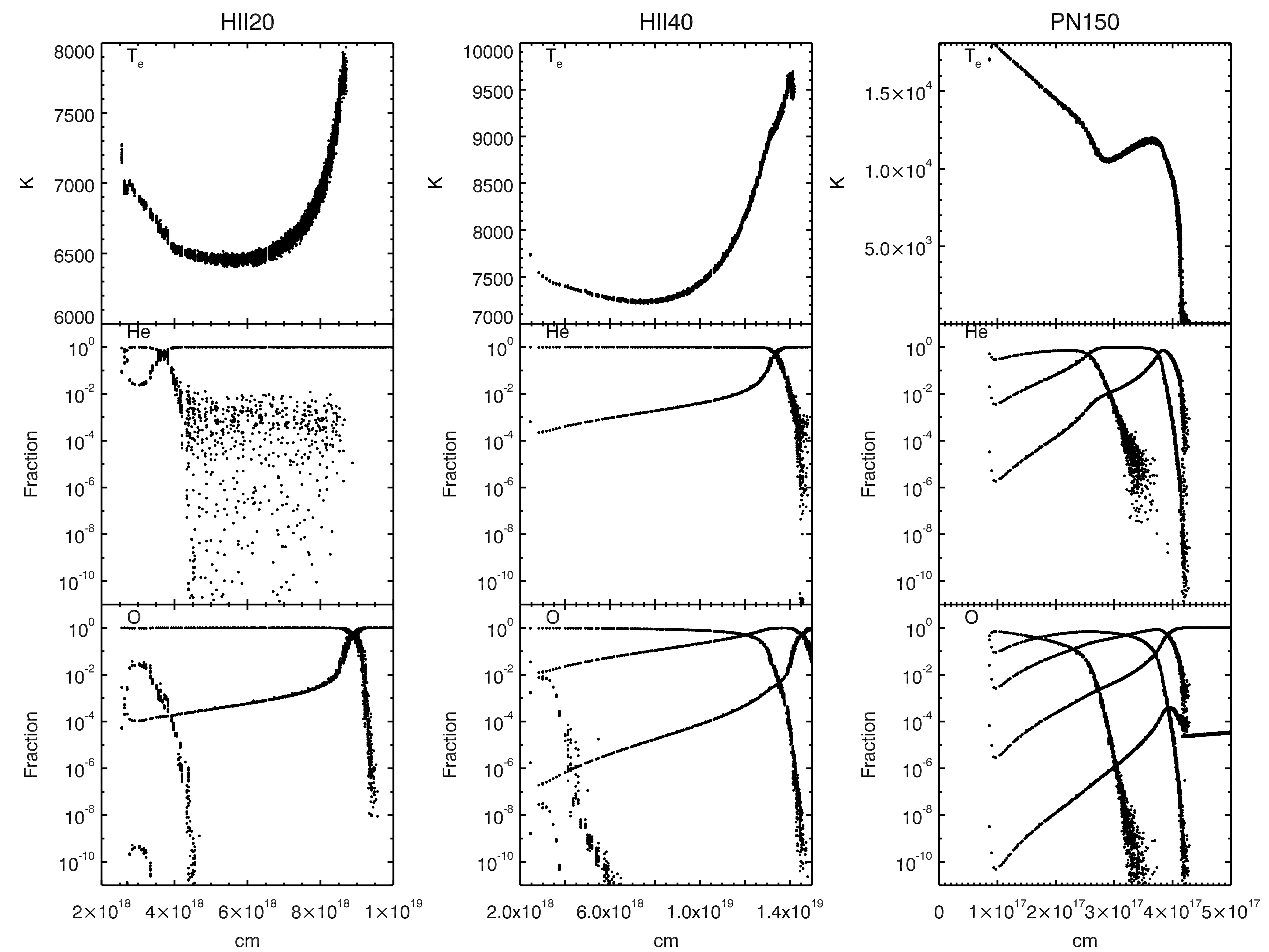
Figure 2: The thermal and ionization structures of HII20, HII40 and PN150 Meudon/Lexington benchmarks. From top to bottom, each row shows the radial profile of the electron temperature and the ionic fraction of He and O.

We apply our $\rm M^{3}$ code to the Lexington/Meudon models. The Lexington/Meudon standard models are a series of artificial cases designed by modellers at the workshops in Meudon, France (Péquignot, 1986) and Lexington, Kentucky, USA (Ferland, 1995), for the purpose of testing the capability of each code in modelling low-temperature, high-temperature Hii regions and planetary nebula.

We run three Lexington/Meudon benchmarks, HII20, HII40 and PN150. All the three benchmarks are run in a low-resolution mode with $33^{3}$ cells and a high-resolution mode with $55^{3}$ cells. All the models are run on the computer with a 2.9-3.3GHz CPU. The HII20 model represents the physical conditions in low-temperature Hii regions with 20000 K and the HII40 model represents high-temperature Hii regions with 40000 K. The PN150 model is representative of planetary nebulae which have hard ionization fields compared to normal Hii regions. The details of each model are listed in Table 1.

Figure 2 presents the radial profiles of electron temperature and the ionic fraction predicted by $\rm M^{3}$. We reproduce the tight temperature and ionic fraction profiles. The $\rm He^{+}$ fraction scatters largely beyond the $\rm He^{+}$ ionizing front in the HII20 model, which is from the residual ionization caused by charge exchange reactions between hydrogen and helium. However, the value of $\rm He^{+}$ fraction is below $\rm 1$ per cent, which has no impact on the temperature, electron density and emission-line fluxes.

Predicted emission-line fluxes are listed in Table 2 to Table 4. We also show the results given by other photoionization codes and calculate median fluxes for each emission-line as a reference. These reference photoionization codes are cloudy (Ferland, 1995, hereafter GF), mappings v (Sutherland & Dopita, 1993, hereafter RS), mocassin3d (Ercolano et al., 2003, hereafter BE), nebula (Rubin et al., 1991, hereafter RR) and P. Harrington’s code (hereafter PH). cloudy and mappings v are two popular one-dimensional photoionization codes using the $outward$-$only$ approximation on the treatment of diffuse radiation field. The RR and PH codes are chosen because they are the only two codes solving the diffuse radiation transfer by iterative calculations. mocassin3d is a Monte Carlo photoionization code developed with a different treatment of microphysics. Compared with mocassin3d, $\rm M^{3}$ has a more comprehensive consideration of the ionization and recombination processes in the ISM.

In the HII20 and PN150 models, all emission-line fluxes predicted by $\rm M^{3}$ are within $\rm 2\sigma$ deviation to the reference fluxes. In the low-resolution mode HII40 model, [O i]$\lambda 6300+6363$ and [S ii]$\lambda 6716+6731$ are $\rm 2-3\sigma$ of the reference emission-line fluxes. In the high-resolution mode HII40 model, the H$\beta$ fluxes are $\rm 2-3\sigma$ of reference emission-line fluxes.

8 The Effect of Spatial Resolution on Emission-Line Fluxes

We compare the emission-line fluxes between the low-resolution and high-resolution $\rm M^{3}$ models. Most emission-line predictions are consistent between the two resolution modes with less than 10 per cent difference in flux. In contrast, the differences in emission-line fluxes are greater than 10 per cent for [O i]$\lambda 6300+6363$, [O ii]$\lambda 7230+7330$, [S ii]$\lambda 6716+6731$ and [S ii]$\lambda 4068+4076$ in the HII40 model, and for [N i]$\lambda 5200+5198$, [O i]$\lambda 63.1\mu m$, [O i]$\lambda 6300+6363$, [Ne ii]$\lambda 12.8\mu m$, Si ii]$\lambda 2335+$, [S ii]$\lambda 6716+6731$ and [S ii]$\lambda 4069+4076$ in the PN150 model. These emission-lines are located at the boundary of photoionized regions, which are sensitive to the spatial resolution of models.

9 Modeling Hii Regions with Complex Geometries

Realistic nebulae display diverse geometries. The geometry of Hii regions can be roughly classified into blister, bipolar, spherical and irregular (De Pree et al., 2005; Deharveng et al., 2015), which correspond to the blister, bipolar, spherical and fractal Hii region models respectively. The spherical Hii region can be modeled by previous one-dimensional photoionization codes. We apply $\rm M^{3}$ to model three fiducial complex geometries of real nebulae, which are blister, bipolar and irregular Hii regions, to display the capability of $\rm M^{3}$ in dealing with complex geometries of nebulae.

9.1 Blister HII regions

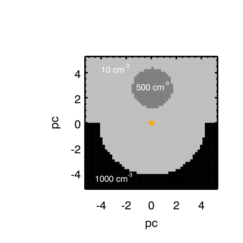
Figure 3: The middle plane (x=0) of the ISM density cube of the blister Hii region model. The black base is the area with the density of hydrogen of 1000 $\rm cm^{-3}$. The dark grey area shows the intermediate density region with the density of 500 $\rm cm^{-3}$. The light grey area is the low density area with the density of 10 $\rm cm^{-3}$.The central orange star indicates the position of the ionizing source.

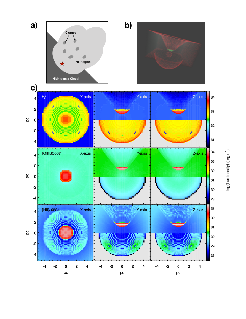
Figure 4: a) Schematic figure of a blister Hii region model. A blister Hii region consists of three major components: a high density cloud base, a intermediate density clumps and the low density ionized gas. b) Three-dimensional visualization of the modeled blister Hii region. c) Distribution of the emission-line luminosity integrated along the x-axis (left), y-axis (middle) and the z-axis (right). We present the distributions of the H$\beta$, [O iii] and [N ii] emission-lines.

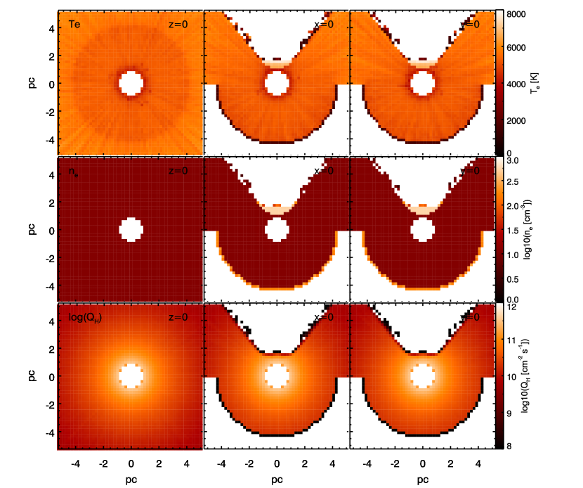
Figure 5: Slices of distributions of the electron temperature, the electron density and the H-ionizing photon flux. We show the cut at z=0 (left), x=0 (middle) and y=0 (right).

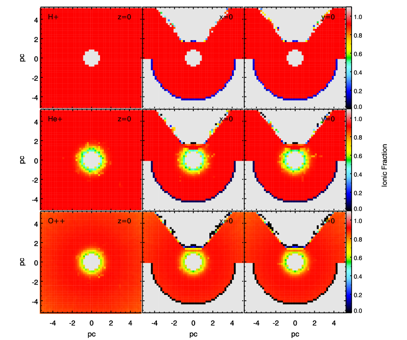
Figure 6: Slices of distributions of $\rm H^{+}$, $\rm He^{+}$ and $\rm O^{++}$. We show the cut at z=0 (left), x=0 (middle) and y=0 (right).

The blister model is a simplified Hii region model, where half of the Hii region is embedded in the dense molecular cloud and half of the Hii region is expelling into the low-dense clumpy ISM (Tenorio-Tagle, 1979; Duronea et al., 2012; Panwar et al., 2020).

Figure 3 shows the input neutral hydrogen density distribution through the middle panel (x=0) of the blister model. The ISM density distribution consists of three parts: a low density component with $n_{H}=10~{}\rm cm^{-3}$, an intermediate density cloud with $n_{H}=500~{}\rm cm^{-3}$ and a high density zone with $n_{H}=1000~{}\rm cm^{-3}$. The value of $\rm 10~{}cm^{-3}$ is consistent with the average density of the hydrogen atom in interstellar space (Brinks, 1990). The intermediate density cloud is designed to reproduce the clumpiness of the ISM. The high density zone is designed as a “bowl-like” shape, consistent with the scenario that blister Hii regions are caused by the stars formed at the edge of the cloud (Gendelev & Krumholz, 2012).

We select a blackbody with temperature of 40000 K as the simple ionizing source. The ionizing source is placed at the center of the simulated domain, with a total luminosity $L_{tot}=3.1\times 10^{39}~{}\rm erg~{}s^{-1}$. The inner radius of nebula is $R_{in}=3\times 10^{18}~{}\rm cm$. We adopt the solar abundance set given by Asplund et al. (2009) (hereafter AS09) as the ISM chemical abundance.

Figure 4 presents the three-dimensional shape of the blister Hii region model. The blister model produces an azimuthally-symmetric nebula consisting of two components. The upper component is the emission from a partially ionized clump and the lower component is the emission from the high density ISM.

$\rm M^{3}$ successfully reproduces the ionization cone and the diffused ionized gas behind the intermediate gas clump. The high density and low density gaseous components represent dense natal molecular clouds and the ionized bubble created by ionization front, stellar wind and photon pressure (Gendelev & Krumholz, 2012). The intermediate density gaseous component represents clumps in the ionized bubble.

We further display the line-of-sight emission-line maps of the blister model in Figure 4 to mimic imaging observations. Similar to spherical nebula models, the Hii region observed along the x-axis has a spherical geometry. However, the integrated emission-line map shows two separate components in views along the y-axis and z-axis.

We trace the distribution of the H$\beta$, [N ii] and [O iii] diagnostic lines given their importance in separating ionization sources and in measuring metallicity and ionization parameters in galaxies and Hii regions. The H$\beta$ and [N ii] spatially coexist within the blister Hii region, where the majority of luminosity are from the high density ISM. The lower component contributes 80 per cent of the total H$\beta$ luminosity and 87 per cent of the total [N ii] luminosity. The [O iii] emission is predominantly from the intermediate density clump which is close to the ionizing source. The clump is partially ionized but contributes 96 per cent of the total [O iii] luminosity.

Figure 5 shows the slices of electron temperature, electron density and H-ionizing photon flux across planes of x=0, y=0 and z=0. The electron temperature, the electron density and the H-ionizing photon flux are uniformly distributed within the main body of the nebula. The main body of the nebula has an average electron temperature of 4000 K and an average electron density of 10 $\rm cm^{-3}$. The intermediate density cloud has a hotter average electron temperature of 6000 K and a higher average electron density of 450 $\rm cm^{-3}$ than the remaining part of the nebula. The average electron temperature in the diffuse ionized gas is 1000 K cooler than the main body of the nebula. The average electron density in the diffuse ionized gas is 10 $\rm cm^{-3}$ similar to the main body of the nebula.

Figure 6 shows the slices of ionic fractions of $\rm H^{+}$, $\rm He^{+}$ and $\rm O^{++}$ across planes of x=0, y=0 and z=0. The $\rm H^{+}$ and $\rm He^{+}$ are dominant ionic species within nebulae and the $\rm O^{++}$ is the major coolant species. The ionic fractions of $\rm H^{+}$, $\rm He^{+}$ and $\rm O^{++}$ are uniformly distributed across the nebula.

9.2 Bipolar HII regions

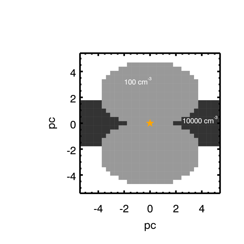
Figure 7: The middle plane (x=0) of the ISM density cube of the bipolar Hii region model. The black area represents the sheet-like high density cloud with the density of hydrogen of 10000 $\rm cm^{-3}$. The grey area shows the ionized gas with the density of 100 $\rm cm^{-3}$.The central orange star indicates the position of the ionizing source.

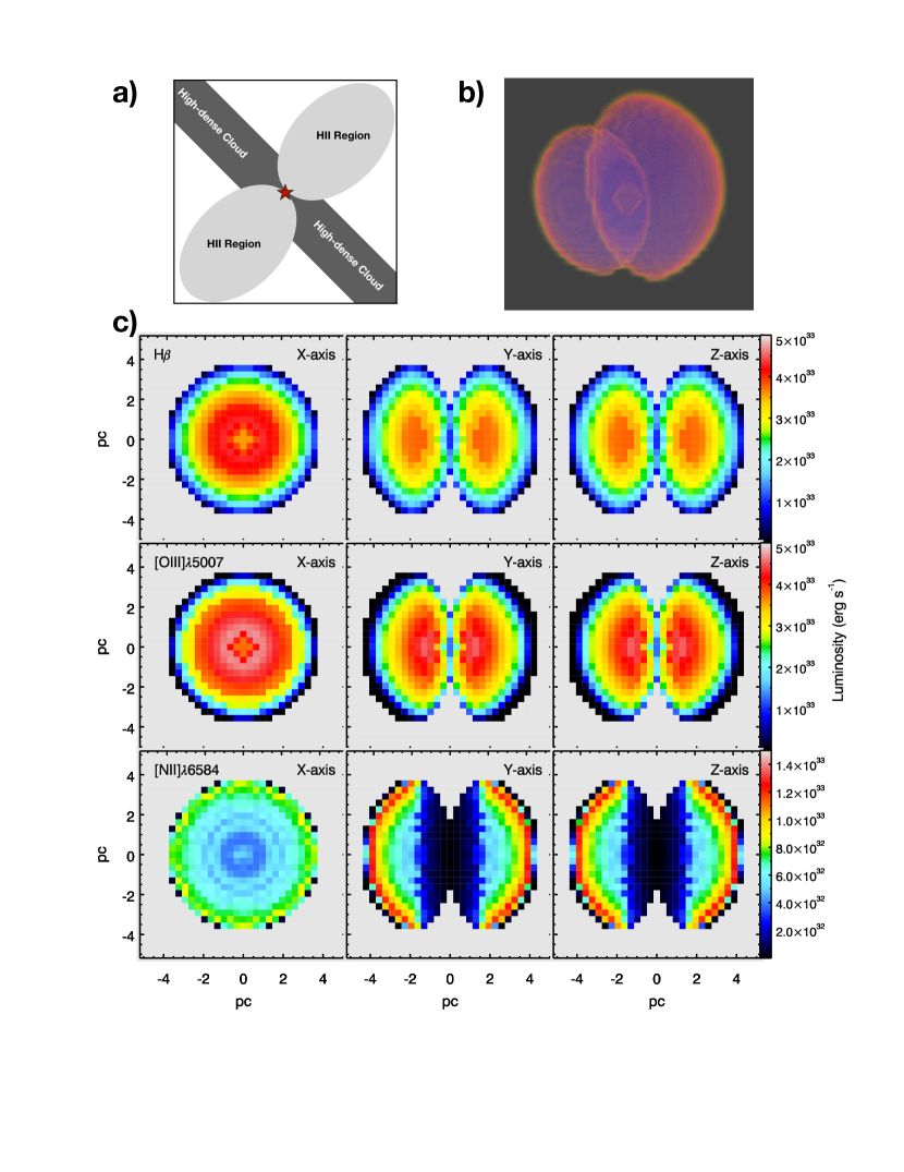
Figure 8: a) Schematic figure of a bipolar Hii region model. A bipolar Hii region consists of two major components: a high-dense sheet-like cloud, the low-dense ionized gas. b) Three-dimensional visualization of the modeled bipolar Hii region. c) Distribution of the emission-line luminosity integrated along the x-axis (left), y-axis (middle) and the z-axis (right). We present the distributions of the H$\beta$, [O iii] and [N ii] emission-lines.

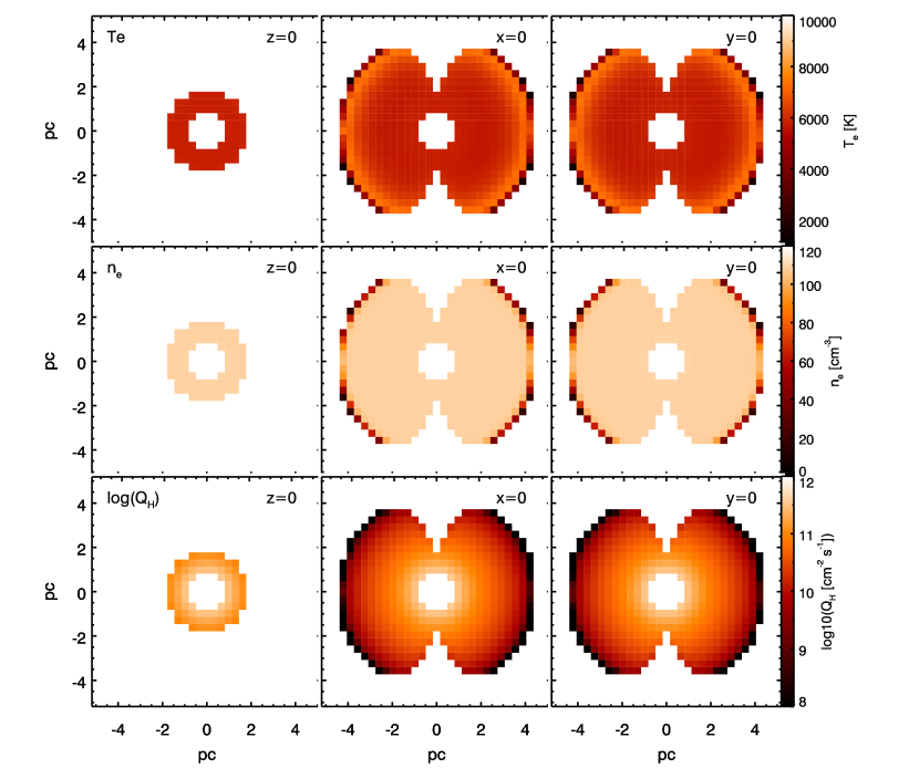
Figure 9: Slices of distributions of the electron temperature, the electron density and the H-ionizing photon flux. We show the cut at z=0 (left), x=0 (middle) and y=0 (right).

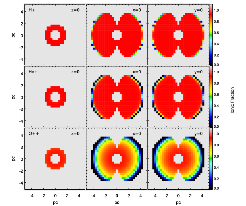
Figure 10: Slices of distributions of $\rm H^{+}$, $\rm He^{+}$ and $\rm O^{++}$. We show the cut at z=0 (left), x=0 (middle) and y=0 (right).

The bipolar Hii region model is composed of two ionized lobes located perpendicularly to a dense molecular cloud (Samal et al., 2018). Three-dimensional simulations suggest that the bipolar structure is the consequence of a star evolving in a sheet-like molecular cloud (Bodenheimer et al., 1979; Wareing et al., 2017).

Figure 7 shows the initial condition of neutral hydrogen density distribution through the middle panel (x=0) of the bipolar Hii region model. The ISM density distribution consists two lobes with $n_{H}=100~{}\rm cm^{-3}$ oriented perpendicular to a sheet-like high density cloud with $n_{H}=10000~{}\rm cm^{-3}$. The density of $\rm 100~{}cm^{-3}$ within two lobes is selected to match with the typical density of local nebula in star-forming galaxies (Kewley et al., 2001; Levesque et al., 2010). The density of the high density cloud is selected based on data that indicate that the sheet-like clouds have density of $\rm 10^{4}~{}cm^{-3}$ (Deharveng et al., 2015).

The central ionizing source is selected as a blackbody with temperature of 40000 K and a total luminosity $L_{tot}=3.1\times 10^{39}~{}\rm erg~{}s^{-1}$. The inner radius of nebula is $R_{in}=3\times 10^{18}~{}\rm cm$. The ISM chemical abundance is the AS09 solar abundance.

Figure 8 presents the three-dimensional shape of the bipolar Hii region model. We present the line-of-sight distribution of the integrated H$\beta$, [O iii] and [N ii] emission-lines. The H$\beta$ and [O iii] emissions are filled in the bipolar lobes appearing as two bubble structures. By contrast, the [N ii] emissions are mainly located on the surface of the bipolar lobes, appearing to be a shell-like morphology.

The bubble structures in the bipolar model exist in most Hii regions (Churchwell et al., 2007; Deharveng et al., 2015). Bipolar structures may appear as ring-like structures if the nebulae are observed in particular viewing angles (Anderson et al., 2011). The 3D visualization of our bipolar model presents ring-like structures similar to real observations.

Figure 9 shows the slices of electron temperature, electron density and H-ionizing photon flux across planes of x=0, y=0 and z=0. The radial profiles of electron temperature, electron density and H-ionizing photon flux in the bipolar nebula are similar to the profiles of the spherical model, where the electron temperature, the electron density and the H-ionizing photon flux have flat gradients within the nebula. The average electron density is 108 $\rm cm^{-3}$ and the average electron temperature is 6000 K. The electron density is reduced and the electron temperature becomes cooler at the edge of the nebula because the ionizing photons are totally absorbed.

Figure 10 shows the slices of ionic fractions of $\rm H^{+}$, $\rm He^{+}$ and $\rm O^{++}$ across planes of x=0, y=0 and z=0. The ionic fractions of $\rm H^{+}$ and $\rm He^{+}$ are uniformly distributed in the nebula. In contrast, the ionic fraction of $\rm O^{++}$ decreases along with the radius of the nebula.

9.3 Fractal Geometry HII regions

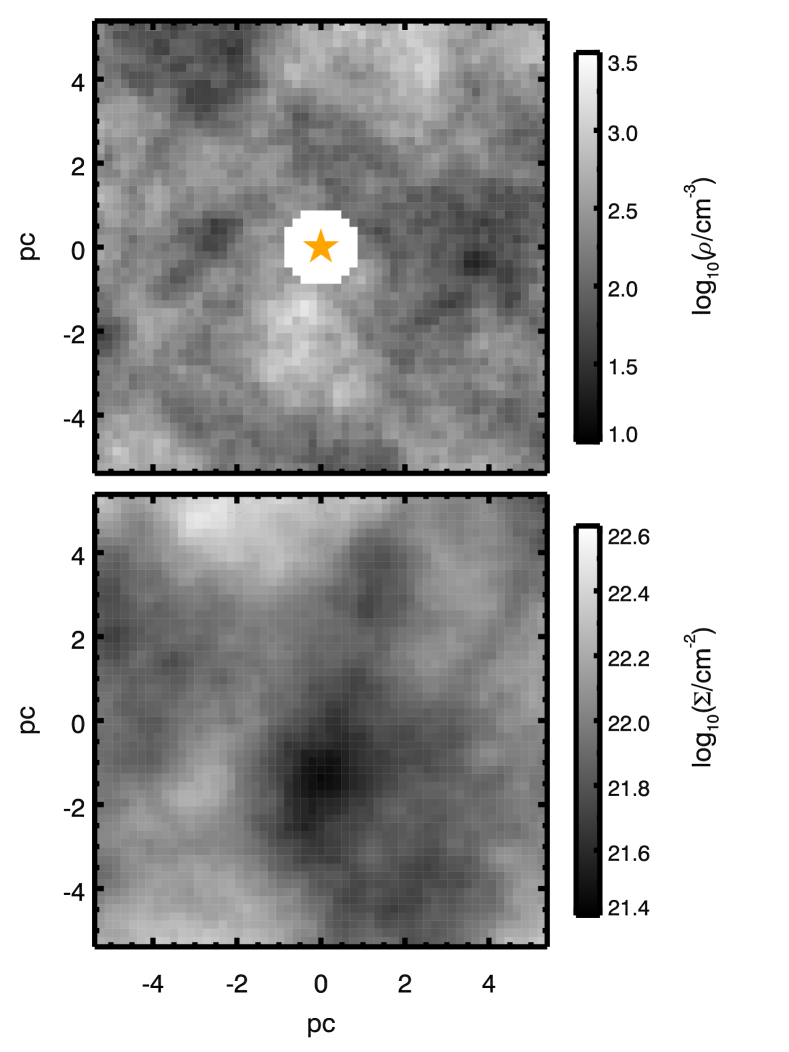
Figure 11: Density distribution of the fractal ISM set up for the fractal Hii region model. The top panel is the middle plane of the input cube of number density, $\rho$. The central cavity corresponds to an inner radius $R_{in}=3\times 10^{18}~{}\rm cm$. The orange star indicates the position of the ionizing source. The bottom panel shows the column number density, $\Sigma$, of the input fractal ISM.

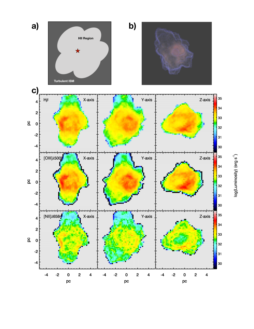
Figure 12: a) Schematic figure of a fractal Hii region model. A fractal Hii region is embedded in the turbulent ISM. b) Three-dimensional visualization of the modeled fractal Hii region. c) Distribution of the emission-line luminosity integrated along the x-axis (left), y-axis (middle) and the z-axis (right). We present the distributions of the H$\beta$, [O iii] and [N ii] emission-lines.

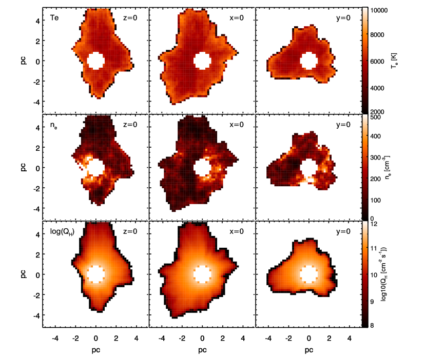
Figure 13: Slices of distributions of the electron temperature, the electron density and the H-ionizing photon flux. We show the cut at z=0 (left), x=0 (middle) and y=0 (right).

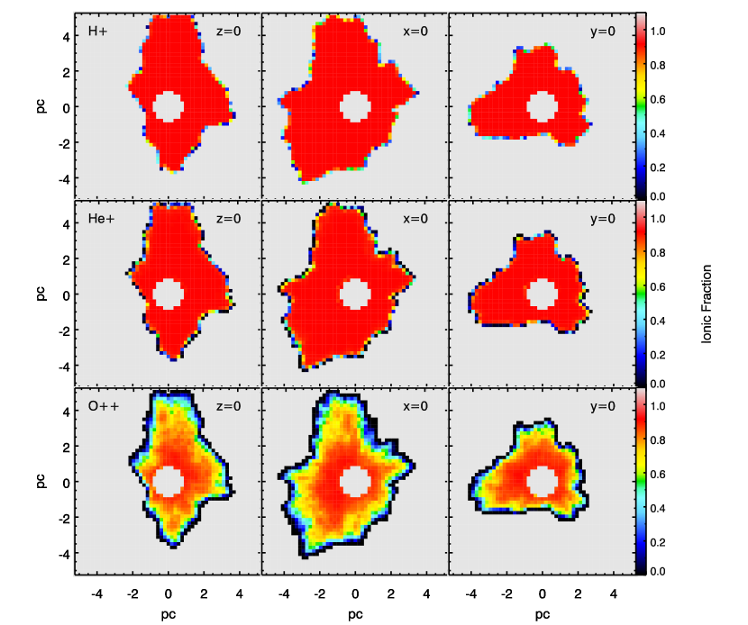
Figure 14: Slices of distributions of $\rm H^{+}$, $\rm He^{+}$ and $\rm O^{++}$. We show the cut at z=0 (left), x=0 (middle) and y=0 (right).

The fractal Hii region model represents an Hii region evolving in the turbulent ISM (Medina et al., 2014) and developing self-similar structures (Zuckerman, 1973; Rubin et al., 2011; Arthur et al., 2016; O’Dell et al., 2017). Both observations (Wisnioski et al., 2015) and simulations (Pillepich et al., 2019) reveal that the turbulent motion dominates the ISM kinematics especially in high-redshift galaxies.

Figure 11 shows the neutral hydrogen density distribution in the fractal model. Following the Kolmogorov’s theory (Kolmogorov, 1941), the power spectrum of the turbulence is in the format of $E(k)\propto k^{-5/3}$, where $k$ is the wavenumber $k\sim 1/r$. The column density probability distribution function (PDF) of the ISM is designed as the log-normal distribution because of the hierarchical structures of the turbulent ISM (Larson, 1981). The mean value of the column density is 100 $\rm cm^{-3}$. We use AS09 for the ISM chemical abundances. The central ionizing source is a blackbody with temperature of 40000 K and a total luminosity $L_{tot}=3.1\times 10^{39}~{}\rm erg~{}s^{-1}$. The inner radius of nebula is $R_{in}=3\times 10^{18}~{}\rm cm$.

Figure 12 displays the shape of the fractal Hii region model in three-dimensions. The modeled Hii region has an inhomogeneous geometry which is caused by the fractal density distribution of the ISM.

Theories suggest that a turbulent model best describes the ISM which has a fractal density distribution (Federrath et al., 2009). $\rm M^{3}$ successfully reproduces the fractal Hii region model with an inhomogeneous density distribution and non-uniform emission-line distributions, which neither spherical models nor plane-parallel models can produce.

We also present the line-of-sight integrated emission-line maps of the fractal model. The Hii region morphology changes in different line-of-sight views. In each line-of-sight direction, the H$\beta$ and [O iii] share the similar spatial distribution, which are concentrated around the center of the nebula. Compared with the H$\beta$ and [O iii], the [N ii] is less concentrated to the central source because the high local ionization parameter ionizes $\rm N^{+}$ to higher ionization levels.

Figure 13 shows the slices of electron temperature, electron density and H-ionizing photon flux across planes of x=0, y=0 and z=0. The electron temperature and the H-ionizing photon flux are uniformly distributed across the nebula. In contrast, the electron density distribution shows a large fluctuation, where the high density ISM has the high electron density and the low density ISM has the low electron density. The average electron density is 150 $\rm cm^{-3}$ with the standard deviation of 90 $\rm cm^{-3}$.

Figure 14 shows the slices of ionic fractions of $\rm H^{+}$, $\rm He^{+}$ and $\rm O^{++}$ across planes of x=0, y=0 and z=0. The ionic fractions of $\rm H^{+}$ and $\rm He^{+}$ are uniformly distributed across the model. The ionic fraction of $\rm O^{++}$ decreases as a function of the nebular radius.

10 Comparison Between Models with Complex Geometries and Spherical Models

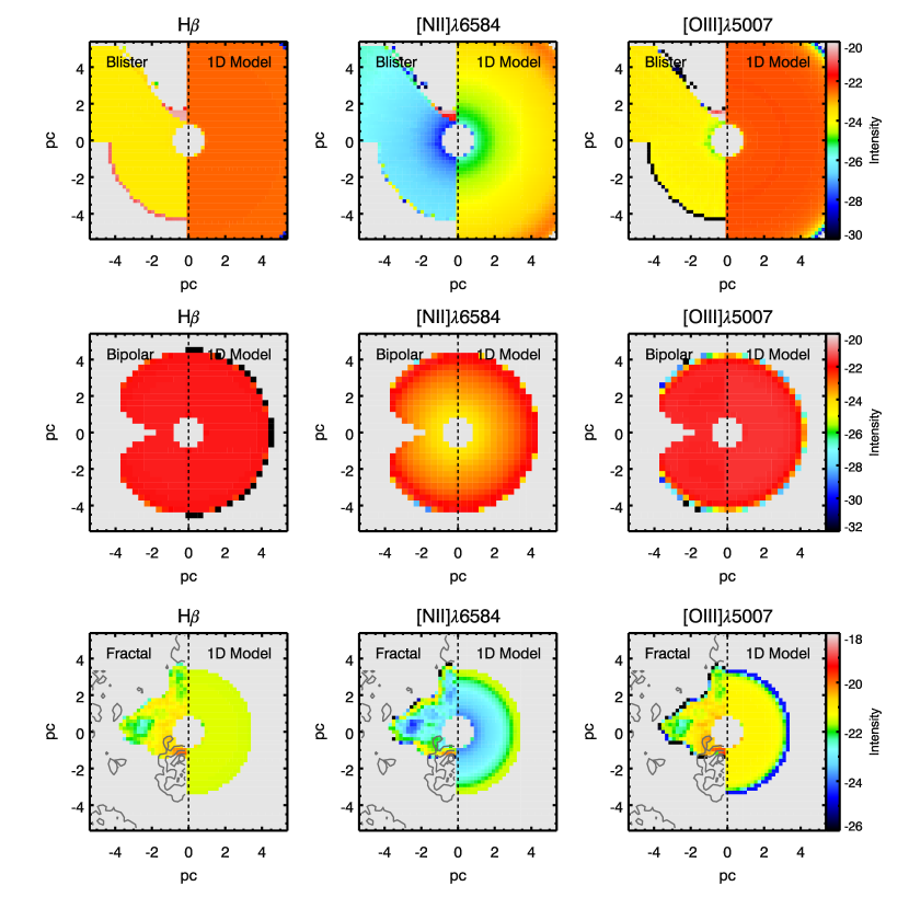
Figure 15: Comparison of the emission-line distribution between the nebular models with complex geometries and the corresponding spherical models. In each panel, the left side shows the cut of the emission-line distribution of the model with complex geometry. The right side shows the cut of the emission-line distribution of the spherical model.

Figure 16: Comparison of integrated emission-line fluxes (left) and emission-line ratios (right) between the models with complex geometries and the spherical models. The horizon dashed line indicates that the integrated fluxes or emission-line ratios from models with complex geometry and from spherical models are the same.

We create a corresponding spherical model for the blister, bipolar and fractal nebula models respectively. Except for the geometry, the spherical model has the same initial conditions as the geometric models, including the ionizing source, the ISM abundance, the total mass of nebula and the average ISM density. The corresponding spherical models to the blister and bipolar Hii regions are radiation-bounded because the radiation field is absorbed before reaching the edge of ISM. The corresponding spherical model to the fractal Hii region is density-bounded, because the ISM density inhomogeneity may shorten the radiation field.

Figure 15 presents the comparison of emission-line distributions between the geometric models and the spherical models. The spherical models have the obvious stratification of emission-line distributions, where the [N ii] lines are located at the boundary of the nebula and the [O iii] lines are mainly from the center of the nebula. By contrast, the density fluctuations in nebulae with complex geometries smooth the stratification of internal distributions of emission-lines.

Figure 16 further shows the changes of integrated emission-line fluxes between the models with complex geometries and the spherical models. Different nebular geometries change the integrated emission-line fluxes in different directions. Compared to the spherical model, the “Blister” geometry reduces the integrated fluxes of [O iii] and [N ii] by around 80% and the integrated flux of H$\beta$ by around 35%. In the bipolar model, the bipolar structure reduces the integrated fluxes of [O iii] and [N ii] by 30-40%. However, the bipolar model has similar integrated flux of H$\beta$ compared to the spherical model. The fractal geometry affects integrated fluxes in the opposite direction. Compared to the spherical model, the fractal geometry increases the integrated flux of [N ii] by around 30% and the integrated flux of H$\beta$ by around 10%. The fractal geometry slightly reduces the integrated flux of [O iii] by 10% compared to the spherical model.

11 Discussion

11.1 Electron Temperature Structure of HII regions

Realistic Hii regions have significant temperature fluctuations within the nebulae (Rubin et al., 2011; Peimbert, 2019). Detailed observations of $\theta^{1}$ Ori C in the Orion Nebula show that the electron temperature has an increasing trend with the distance from the ionizing star. In current constant density photoionization models, the electron temperature becomes hotter towards the edge of Hii regions when the metallicity of nebulae $\rm 12+log(O/H)\geq 8.5$ (Kewley et al., 2019).

The mechanisms leading to the electron temperature fluctuations are still under debate. Multiple mechanisms have been proposed, including the turbulence and shocks in the ISM (Peimbert et al., 1991; O’Dell et al., 2015), and the stellar winds produced by central ionizing sources (Gonzalez-Delgado et al., 1994)

Here we propose that the nebular geometry is one, but not the only cause of the electron temperature fluctuation. The degree of electron temperature fluctuation increases with the complexity of nebular geometry. The electron temperature in the blister and bipolar Hii region models has a flat gradient because the hydrogen density is uniformly distributed within ionized bubbles. In the blister Hii region model, the intermediate density clump is hotter than the average electron temperature of the nebula because the clump is denser than the average density of the nebula. The fractal Hii region model has a more significant electron temperature fluctuation than the blister and bipolar Hii region models, because the self-hierarchical structure in the fractal model is the most complex geometry among the blister, bipolar and fractal models.

Nebula models allowing the electron temperature fluctuation offers great promise in interpreting emission-line spectra. The spectra of nearby or distant galaxies captured by fixed-size apertures combine the light from an ensemble of Hii regions with complex electron temperature structures. The electron temperature fluctuation is a potential cause of the discrepancy between the metallicity determined by recombination lines and those determined with Auroral lines (Peimbert, 2019). The turbulent ISM in high-redshift galaxies increase the electron temperature fluctuations of nebulae. Three-dimensional nebula models with complex electron temperature structures provide more realistic predictions of emission-lines than those models with constant temperature, density or pressure assumptions.

11.2 Density Structure of HII regions

Realistic nebulae have significant density fluctuations within local Hii regions (Pérez et al., 2001; Simpson et al., 2004; McLeod et al., 2016; Peimbert, 2019). Spatially-resolved measurements show negative density gradients in some local Hii regions (Kurtz, 2002; Phillips, 2007; Rubin et al., 2011) and flat density gradients in other compact Hii regions (García-Benito et al., 2010; Ramos-Larios et al., 2010). Detailed observations of the Orion Nebula find that the turbulence within the nebula leads to the complex density structures (Arthur et al., 2016; O’Dell et al., 2017; Kewley et al., 2019).

We present diverse electron density distributions in three fiducial Hii region models. The bipolar Hii region model presents a flat electron density gradient because the density distribution of hydrogen is uniform within the bipolar bubbles. The blister and fractal Hii regions present significant electron density fluctuations, which are caused by the inhomogeneity of the ISM density within the nebulae.

11.3 Emission-Line Predictions

The [O iii]$\lambda 5007$, [N ii]$\lambda 6584$ and H$\beta$ are crucial diagnostic emission-lines for galaxy evolution study. These three emission-lines have different dependance on the nebular geometry. The [O iii]$\lambda 5007$ and H$\beta$ are produced throughout the entire nebula, and their fluxes are sensitive to the size of nebular volume. The [N ii]$\lambda 6584$ traces the intermediate-ionization zone of nebula, which is located at the more outer region than the [O iii]$\lambda 5007$ and H$\beta$. The flux of [N ii]$\lambda 6584$ is more sensitive to the length of nebular boundary than the fluxes of [O iii]$\lambda 5007$ and H$\beta$.

Complex geometry affects the emission-line predictions. The twisted boundary and the irregular shape of the nebula changes the fluxes of [O iii]$\lambda 5007$, [N ii]$\lambda 6584$ and H$\beta$. The inhomogeneity of ISM density changes the spatial distributions of emission-lines within nebulae, which cannot be reproduced by nebula models with spherical or plane parallel geometries. We will investigate the detailed impact of nebular geometry on the optical emission-lines in a forthcoming paper (Jin et al. in prep).

Oversimplified nebular geometries in emission-line modelings lead to the debate on how the nebulae are bounded. Spherical and plane parallel nebula models assume that Hii regions are simply radiation-bounded, in order to reproduce the observed emission-line fluxes in nearby galaxies (Kewley et al., 2001). However, Nakajima et al. (2013) proposed that the Hii regions in high-redshift galaxies are likely to be density-bounded, where the gas is insufficient to absorb the entire ionizing photons from the star. Detailed studies of nearby Hii regions suggest that the radiation-bounded and density-bounded conditions coexist within a single nebula (Pellegrini et al., 2012).

$\rm M^{3}$ can produce emission-lines in Hii region models with complex geometries, allowing a mixture of radiation-bounded and density-bounded cases. Among the three fiducial nebula models, the bipolar Hii region model and the fractal Hii region model are simply radiation-bounded cases. The blister Hii region model is a mixture of radiation-bounded and density-bounded nebula, where the nebula is radiation-bounded in the high density zone and the intermediate density cloud, and the nebula is density-bounded in the low density gaseous component.

12 Conclusion

$\rm M^{3}$ is a photoionization code designed for modeling the Hii regions with arbitrary three-dimensional geometries. $\rm M^{3}$ incorporates the Monte Carlo radiative transfer technique with the complete ISM microphysics implemented in mappings v code, producing realistic three-dimensional ionization and thermal structures within nebulae. The accurate cooling functions in $\rm M^{3}$ promise reliable predictions of the emission-line fluxes.

We put $\rm M^{3}$ successfully through the Lexington/Meudon benchmarks test, which is a series of artificial photoionized models accounting for the physical conditions of various types of Hii regions and planetary nebulae. The emission-line fluxes predicted by $\rm M^{3}$ are consistent with the fluxes produced by the reference photoionization codes. We run each Lexington/Meudon benchmark with a high-resolution mode and a low-resolution mode, finding the spatial resolution effect is pronounced for emission-line fluxes produced at the edge of Hii regions.

We create three fiducial Hii region models with complex geometries, which are the blister geometry, the bipolar geometry and the fractal geometry. We find that:

• In the blister Hii region model, the high-density clump is partially ionized. The high-density clumpy structure has hotter electron temperature and higher electron density than the low-density gas in the nebula. The diffuse ionized gas is partially ionized and cooler than the average electron temperature of the nebula.

• The bipolar Hii region model has the similar radial profiles to the spherical model, in terms of the electron temperature, the electron density, the ionizing photon flux, the ionic fraction and the emission-line intensities. However, the bipolar Hii region has smaller volume size than the spherical model, reducing the integrated emission-line fluxes.

• The fractal model has the most complex geometry among the three fiducial Hii region models. Neither the internal ionization and thermal structures nor the integrated emission-line fluxes can be reproduced by simple spherical photoioinzation models. The inhomogeneity of ISM density causes the fluctuation of the electron temperature and the electron density. The twisted nebular boundary of the fractal model increase the boundary emission-line species.

We demonstrate that $\rm M^{3}$ is a promising tool for interpreting nebular emission-line behaviors in the era of JWST and the upcoming local integral-field unit surveys, like SDSS-V/LVM (the Local Volume Mapper).

We are grateful for the valuable comments on this work by an anonymous referee that improved the scientific outcome and quality of the paper. This research was conducted on the traditional lands of the Ngunnawal and Ngambri people. YFJ is grateful to Brent Groves, Christoph Federrath, Emily Wisnioski and David Nicholls for useful discussions. This research was supported by the Australian Research Council Centre of Excellence for All Sky Astrophysics in 3 Dimensions (ASTRO 3D), through project number CE170100013. L.J.K. gratefully acknowledges the support of an ARC Laureate Fellowship (FL150100113).

Table 1: The Lexington/Meudon benchmarks

	HII20	HII40	PN150
$\Phi_{H}~{}(10^{47}\rm photon~{}s^{-1})$	100.0	426.6	5.4
$T_{eff}~{}(\rm kK)$	20	40	150
$n_{H}~{}(\rm cm^{-3})$	100	100	3000
$R_{in}~{}(\rm cm)$	3$\times\rm 10^{18}$	3$\times\rm 10^{18}$	1$\times\rm 10^{17}$
He	0.1	0.1	0.1
C	2.2$\times\rm 10^{-4}$	2.2$\times\rm 10^{-4}$	3.0$\times\rm 10^{-4}$
N	4.0$\times\rm 10^{-5}$	4.0$\times\rm 10^{-5}$	1.0$\times\rm 10^{-4}$
O	3.3$\times\rm 10^{-4}$	3.3$\times\rm 10^{-4}$	6.0$\times\rm 10^{-4}$
Ne	5.0$\times\rm 10^{-5}$	5.0$\times\rm 10^{-5}$	1.5$\times\rm 10^{-4}$
Mg	–	–	3.0$\times\rm 10^{-5}$
Si	–	–	3.0$\times\rm 10^{-5}$
S	9.0$\times\rm 10^{-6}$	9.0$\times\rm 10^{-6}$	1.5$\times\rm 10^{-5}$
CPU Time ($33^{3}$ cells)	04h14m13s	05h28m12s	07h03m12s
CPU Time ($55^{3}$ cells)	23h55m33s	19h56m32s	29h53m25s

Table 2: Meudon/Lexington H ii Region Benchmark Results: HII20. The $\rm M^{3}$($33^{3}$) and $\rm M^{3}$($55^{3}$) are the results of the low-resolution model and the high-resolution model respectively. $\Delta\%$ is the deviation of the results between $\rm M^{3}$($33^{3}$) and $\rm M^{3}$($55^{3}$). “Med” column shows the medium value and 1-$\sigma$ deviation of the results given by mappings, cloudy, mocassin3d, RR and PH codes.

Line/H$\beta$	$\rm M^{3}$($33^{3}$)	$\rm M^{3}$($55^{3}$)	$\Delta\%$	mappings	cloudy	mocassin3d	RR	PH	Med$\pm\sigma$
H$\beta$ ($\rm 10^{36}erg~{}s^{-1}$)	4.81	4.81	0.00	5.04	4.85	4.97	4.89	4.93	4.89$\pm$0.09
He i 5876	0.0071	0.0071	0.00	0.0110	0.0072	0.0065	–	0.0074	0.0072$\pm$0.0016
C ii] 2325+	0.059	0.059	0.00	0.038	0.054	0.042	0.063	0.060	0.059$\pm$0.010
[N ii] 122$\mu$m	0.072	0.072	0.00	0.071	0.068	0.071	0.071	0.072	0.071$\pm$0.001
[N ii] 6584+6548	0.783	0.783	0.00	0.803	0.745	0.846	0.915	0.843	0.803$\pm$0.056
[N ii] 5755	0.0028	0.0028	0.00	0.0030	0.0028	0.0025	0.0033	0.0033	0.0028$\pm$0.0003
[N iii] 57.3$\mu$m	0.0028	0.0027	3.57	0.0020	0.0040	0.0019	0.0022	0.0031	0.0027$\pm$0.0007
[O i] 6300+6363	0.0239	0.0241	0.84	0.0050	0.0080	0.0088	–	0.0047	0.0088$\pm$0.0091
[O ii] 7320+7330	0.0064	0.0064	0.00	0.0080	0.0087	0.0064	0.0100	0.0103	0.0080$\pm$0.0017
[O ii] 3726+3729	1.24	1.24	0.00	1.08	1.01	0.909	1.17	1.22	1.17$\pm$0.13
[O iii] 52+88$\mu$m	0.0030	0.0029	3.33	0.0020	0.0030	0.0022	0.0017	0.0037	0.0029$\pm$0.0007
[O iii] 5007+4959	0.0019	0.0019	0.00	0.0010	0.0021	0.0011	0.0010	0.0014	0.0014$\pm$0.0005
[Ne ii] 12.8$\mu$m	0.296	0.296	0.00	0.286	0.264	0.295	0.290	0.271	0.290$\pm$0.013
[S ii] 6716+6731	0.528	0.529	0.19	0.435	0.499	0.486	0.492	0.555	0.499$\pm$0.039
[S ii] 4068+4076	0.015	0.016	6.67	0.012	0.022	0.013	0.015	0.017	0.015$\pm$0.003
[S iii] 18.7$\mu$m	0.324	0.324	0.00	0.398	0.445	0.371	0.374	0.365	0.371$\pm$0.042
[S iii] 9532+9069	0.442	0.441	0.23	0.604	0.501	0.526	0.551	0.549	0.526$\pm$ 0.060

Table 3: Meudon/Lexington H ii Region Benchmark Results: HII40.

Line/H$\beta$	$\rm M^{3}$($33^{3}$)	$\rm M^{3}$($55^{3}$)	$\Delta\%$	mappings	cloudy	mocassin3d	RR	PH	Med$\pm\sigma$
H$\beta$ ($\rm 10^{37}erg~{}s^{-1}$)	2.00	1.98	1.00	2.07	2.06	2.02	2.05	2.05	2.05$\pm$0.03
He i 5876	0.117	0.115	1.71	0.116	0.119	0.114	–	0.118	0.116$\pm$0.047
C ii] 2325+	0.170	0.164	3.53	0.096	0.157	0.148	0.178	0.166	0.164$\pm$0.027
C iii] 1907+1909	0.076	0.076	0.00	0.066	0.071	0.041	0.074	0.060	0.071$\pm$0.013
[N ii] 122$\mu$m	0.030	0.029	3.33	0.035	0.027	0.036	0.030	0.032	0.030$\pm$0.003
[N ii] 6584+6548	0.647	0.632	2.32	0.723	0.669	0.852	0.807	0.736	0.723$\pm$0.082
[N ii] 5755	0.0053	0.0053	0.00	0.0050	0.0050	0.0061	0.0068	0.0064	0.0053$\pm$0.0007
[N iii] 57.3$\mu$m	0.294	0.297	1.02	0.273	0.306	0.223	0.301	0.292	0.294$\pm$0.029
[O i] 6300+6363	0.0425	0.0290	31.76	0.0070	0.0094	0.0065	–	0.0059	0.0094$\pm$0.015
[O ii] 7320+7330	0.020	0.027	35.00	0.024	0.029	0.025	0.036	0.032	0.027$\pm$0.005
[O ii] 3726+3729	2.08	2.05	1.44	1.88	1.94	1.92	2.26	2.19	2.05$\pm$0.14
[O iii] 52+88$\mu$m	2.52	2.55	1.19	2.29	2.35	2.28	2.34	2.34	2.34$\pm$0.11
[O iii] 5007+4959	2.35	2.37	0.85	2.17	2.21	1.64	2.08	1.93	2.17$\pm$0.26
[O iii] 4363	0.00419	0.00421	2.68	0.0040	0.00235	0.0022	0.0035	0.0032	0.0035$\pm$0.0008
[Ne ii] 12.8$\mu$m	0.202	0.199	1.49	0.217	0.177	0.212	0.196	0.181	0.199$\pm$0.015
[Ne iii] 15.5$\mu$m	0.287	0.290	1.05	0.350	0.294	0.267	0.417	0.429	0.294$\pm$0.066
[Ne iii] 3869+3968	0.068	0.069	1.47	0.083	0.084	0.053	0.086	0.087	0.083$\pm$0.013
[S ii] 6716+6731	0.251	0.194	22.71	0.133	0.137	0.141	0.130	0.155	0.141$\pm$0.045
[S ii] 4068+4076	0.0108	0.0086	20.37	0.005	0.0093	0.0060	0.0060	0.0070	0.0070$\pm$0.0021
[S iii] 18.7$\mu$m	0.526	0.534	1.52	0.567	0.627	0.574	0.580	0.556	0.567$\pm$0.033
[S iii] 9532+9069	1.02	1.04	1.96	1.25	1.13	1.21	1.28	1.23	1.21$\pm$0.10

Table 4: Meudon/Lexington H ii Region Benchmark Results: PN150.

Line/H$\beta$	$\rm M^{3}$ ($33^{3}$)	$\rm M^{3}$ ($55^{3}$)	$\Delta\%$	mappings	cloudy	mocassin3d	PH	Med$\pm\sigma$
H$\beta$ ($\rm 10^{35}erg~{}s^{-1}$)	2.59	2.59	0.00	2.64	2.86	2.79	2.68	2.68$\pm$0.11
He i 5876	0.099	0.098	1.01	0.095	0.110	0.104	0.096	0.099$\pm$0.006
He ii 4686	0.314	0.314	0.00	–	0.324	0.333	0.333	0.324$\pm$ 0.010
C ii] 2325+	0.215	0.216	0.47	0.141	0.277	0.141	0.450	0.216$\pm$0.115
C ii 1335	0.015	0.014	6.67	–	0.119	0.121	0.119	0.119$\pm$0.058
C iii] 1907+1909	2.18	2.23	2.29	1.89	1.68	1.72	1.74	1.89$\pm$0.24
C iv 1549+	2.22	2.25	1.35	3.12	2.14	2.71	2.09	2.25$\pm$0.41
[N i] 5200+5198	0.032	0.024	25.00	0.005	0.013	0.0067	0.020	0.020$\pm$0.0105
[N ii] 6584+6548	1.18	1.07	9.32	1.17	1.15	1.43	1.35	1.18$\pm$0.14
[N ii] 5755	0.018	0.017	5.55	0.016	0.017	0.022	0.023	0.018$\pm$0.003
N ii] 1749+	0.102	0.099	2.94	0.091	0.106	0.111	0.139	0.106$\pm$0.017
[N iii] 57.3$\mu$m	0.130	0.133	2.31	0.126	0.129	0.120	0.135	0.130$\pm$0.005
N iv] 1487+	0.253	0.255	0.79	0.168	0.199	0.162	0.141	0.199$\pm$0.048
N v 1240+	0.147	0.144	2.04	0.248	0.147	0.147	0.107	0.147$\pm$0.047
[O i] 63.1$\mu$m	0.038	0.028	26.31	0.049	0.024	0.010	0.007	0.028$\pm$0.016
[O i] 6300+6363	0.258	0.154	40.31	0.101	0.144	0.163	0.104	0.154$\pm$0.057
[O ii] 3726+3729	2.38	2.28	4.20	1.75	2.03	2.24	2.66	2.28$\pm$0.31
[O iii] 51.8$\mu$m	1.37	1.40	2.19	1.28	1.30	1.50	1.39	1.39$\pm$0.08
[O iii] 88.3$\mu$m	0.274	0.279	1.82	0.252	0.261	0.296	0.274	0.274$\pm$0.015
[O iii] 5007+4959	22.0	22.4	1.82	16.8	21.4	22.63	20.8	22.00$\pm$2.16
[O iii] 4363	0.168	0.171	1.79	0.109	0.152	0.169	0.155	0.168$\pm$0.023
[O iv] 25.9$\mu$m	4.09	4.13	0.98	4.05	3.45	3.68	4.20	4.09$\pm$0.30
O iv] 1403+	0.181	0.182	0.55	–	0.183	0.203	0.225	0.183$\pm$0.019
O v] 1218+	0.198	0.193	2.53	0.213	0.165	0.169	0.097	0.193$\pm$0.041
[Ne ii] 12.8$\mu$m	0.055	0.042	23.64	0.043	0.028	0.030	0.027	0.042$\pm$0.011
[Ne iii] 15.5$\mu$m	1.90	1.89	0.53	2.71	1.88	2.02	2.76	2.02$\pm$0.42
[Ne iii] 3869+3968	2.33	2.34	0.43	2.56	2.64	2.63	3.04	2.63$\pm$0.26
[Ne iv] 2423+	0.663	0.668	0.75	0.832	0.707	0.749	0.723	0.723$\pm$0.062
[Ne v] 3426+3346	0.195	0.191	2.05	0.591	0.721	0.692	0.583	0.591$\pm$0.241
[Ne v] 24.2$\mu$m	0.304	0.301	0.99	0.195	0.997	1.007	0.936	0.936$\pm$0.393
Mg ii 2798+	2.34	2.24	4.27	0.863	2.22	2.32	0.555	2.240$\pm$0.818
[Mg iv] 4.49$\mu$m	0.136	0.137	0.74	0.115	0.121	0.111	0.042	0.121$\pm$0.035
Si ii] 2335+	0.152	0.170	11.84	0.127	0.160	0.160	–	0.160$\pm$0.016
Si iii] 1892+	0.179	0.185	3.35	0.083	0.446	0.325	0.382	0.325$\pm$0.139
Si iv] 1397+	0.141	0.143	1.42	0.122	0.183	0.214	0.172	0.172$\pm$0.034
[S ii] 6716+6731	0.382	0.311	18.59	0.322	0.359	0.357	0.451	0.359$\pm$0.050
[S ii] 4069+4076	0.057	0.049	14.04	0.050	0.073	0.064	0.077	0.064$\pm$0.012
[S iii] 18.7$\mu$m	0.527	0.526	0.19	0.578	0.713	0.495	0.488	0.527$\pm$0.084
[S iii] 33.6$\mu$m	0.202	0.200	0.99	0.240	0.281	0.210	0.206	0.210$\pm$0.032
[S iii] 9532+9069	2.01	2.02	0.50	2.04	2.07	1.89	1.90	2.02$\pm$0.08
[S iv] 10.5$\mu$m	2.69	2.72	1.12	2.25	2.09	2.25	2.22	2.25$\pm$0.27

References

- Aldrovandi & Pequignot (1973) Aldrovandi, S. M. V. & Pequignot, D. 1973, A&A, 25, 137
- Anderson et al. (2011) Anderson, L. D., Bania, T. M., Balser, D. S., et al. 2011, ApJS, 194, 32. doi:10.1088/0067-0049/194/2/32
- Arnaud & Rothenflug (1985) Arnaud, M. & Rothenflug, R. 1985, A&AS, 60, 425
- Arthur et al. (2016) Arthur, S. J., Medina, S.-N. X., & Henney, W. J. 2016, MNRAS, 463, 2864. doi:10.1093/mnras/stw2165
- Asplund et al. (2009) Asplund, M., Grevesse, N., Sauval, A. J., & Scott, P. 2009, ARA&A, 47, 481
- Baldwin et al. (1981) Baldwin, J. A., Phillips, M. M., & Terlevich, R. 1981, PASP, 93, 5
- Binette et al. (1982) Binette, L., Dopita, M. A., Dodorico, S., et al. 1982, A&A, 115, 315
- Binette et al. (1985) Binette, L., Dopita, M. A., & Tuohy, I. R. 1985, ApJ, 297, 476
- Binette et al. (2012) Binette, L., Matadamas, R., Hägele, G. F., et al. 2012, A&A, 547, A29. doi:10.1051/0004-6361/201219515
- Blandford et al. (1990) Blandford, R. D., Netzer, H., Woltjer, L., et al. 1990, Active Galactic Nuclei, 97
- Bodenheimer et al. (1979) Bodenheimer, P., Tenorio-Tagle, G., & Yorke, H. W. 1979, ApJ, 233, 85. doi:10.1086/157368
- Brinks (1990) Brinks, E. 1990, The Interstellar Medium in Galaxies, 161, 39. doi:10.1007/978-94-009-0595-5_3
- Byler et al. (2020) Byler, N., Kewley, L. J., Rigby, J. R., et al. 2020, ApJ, 893, 1. doi:10.3847/1538-4357/ab7ea9
- Churchwell et al. (2007) Churchwell, E., Watson, D. F., Povich, M. S., et al. 2007, ApJ, 670, 428. doi:10.1086/521646
- Comeron (1997) Comeron, F. 1997, A&A, 326, 1195
- D’Agostino et al. (2019) D’Agostino, J. J., Kewley, L. J., Groves, B. A., et al. 2019, MNRAS, 485, L38. doi:10.1093/mnrasl/slz028
- Davies et al. (2021) Davies, R. L., Förster Schreiber, N. M., Genzel, R., et al. 2021, ApJ, 909, 78. doi:10.3847/1538-4357/abd551
- Deharveng et al. (2015) Deharveng, L., Zavagno, A., Samal, M. R., et al. 2015, A&A, 582, A1. doi:10.1051/0004-6361/201423835
- Del Zanna et al. (2015) Del Zanna, G., Dere, K. P., Young, P. R., et al. 2015, A&A, 582, A56
- De Pree et al. (2005) De Pree, C. G., Wilner, D. J., Deblasio, J., et al. 2005, ApJ, 624, L101
- Dopita et al. (2000) Dopita, M. A., Kewley, L. J., Heisler, C. A., et al. 2000, ApJ, 542, 224. doi:10.1086/309538
- Draine & Kreisch (2018) Draine, B. T. & Kreisch, C. D. 2018, ApJ, 862, 30. doi:10.3847/1538-4357/aac891
- Duronea et al. (2012) Duronea, N. U., Vasquez, J., Cappa, C. E., et al. 2012, A&A, 537, A149. doi:10.1051/0004-6361/201117958
- Elmegreen & Scalo (2004) Elmegreen, B. G. & Scalo, J. 2004, ARA&A, 42, 211
- Ercolano et al. (2003) Ercolano, B., Barlow, M. J., Storey, P. J., & Liu, X.-W. 2003, MNRAS, 340, 1136
- Federrath et al. (2009) Federrath, C., Klessen, R. S., & Schmidt, W. 2009, ApJ, 692, 364. doi:10.1088/0004-637X/692/1/364
- Ferland (1995) Ferland, G. 1995, The Analysis of Emission Lines: A Meeting in Honor of the 70th Birthdays of D. E. Osterbrock & M. J. Seaton, 83
- Ferland et al. (1998) Ferland, G. J., Korista, K. T., Verner, D. A., et al. 1998, PASP, 110, 761. doi:10.1086/316190
- García-Benito et al. (2010) García-Benito, R., Díaz, A., Hägele, G. F., et al. 2010, MNRAS, 408, 2234. doi:10.1111/j.1365-2966.2010.17269.x
- Gaunt (1930) Gaunt, J. A. 1930, Philosophical Transactions of the Royal Society of London Series A, 229, 163
- Gendelev & Krumholz (2012) Gendelev, L. & Krumholz, M. R. 2012, ApJ, 745, 158. doi:10.1088/0004-637X/745/2/158
- Gonzalez-Delgado et al. (1994) Gonzalez-Delgado, R. M., Perez, E., Tenorio-Tagle, G., et al. 1994, ApJ, 437, 239. doi:10.1086/174992
- Gould & Jung (1991) Gould, R. J. & Jung, Y.-D. 1991, ApJ, 373, 271
- Gritschneder et al. (2010) Gritschneder, M., Burkert, A., Naab, T., et al. 2010, ApJ, 723, 971
- Gronenschild & Mewe (1978) Gronenschild, E. H. B. M. & Mewe, R. 1978, A&AS, 32, 283
- Groves et al. (2004) Groves, B. A., Dopita, M. A., & Sutherland, R. S. 2004, ApJS, 153, 9. doi:10.1086/421113
- Harries & Howarth (1997) Harries, T. J. & Howarth, I. D. 1997, A&AS, 121, 15. doi:10.1051/aas:1997110
- Harrington (1968) Harrington, J. P. 1968, ApJ, 152, 943
- Harshan et al. (2020) Harshan, A., Gupta, A., Tran, K.-V., et al. 2020, ApJ, 892, 77. doi:10.3847/1538-4357/ab76cf
- Hoare et al. (2007) Hoare, M. G., Kurtz, S. E., Lizano, S., et al. 2007, Protostars and Planets V, 181
- Kaasinen et al. (2017) Kaasinen, M., Bian, F., Groves, B., Kewley, L. J., & Gupta, A. 2017, MNRAS, 465, 3220
- Kewley et al. (2001) Kewley, L. J., Dopita, M. A., Sutherland, R. S., Heisler, C. A., & Trevena, J. 2001, ApJ, 556, 121
- Kewley & Ellison (2008) Kewley, L. J., & Ellison, S. L. 2008, ApJ, 681, 1183
- Kewley et al. (2019) Kewley, L. J., Nicholls, D. C., Sutherland, R., et al. 2019, ApJ, 880, 16
- Kobulnicky & Kewley (2004) Kobulnicky, H. A. & Kewley, L. J. 2004, ApJ, 617, 240
- Kolmogorov (1941) Kolmogorov, A. 1941, Akademiia Nauk SSSR Doklady, 30, 301
- Kurtz (2002) Kurtz, S. 2002, Hot Star Workshop III: The Earliest Phases of Massive Star Birth, 267, 81
- Larson (1981) Larson, R. B. 1981, MNRAS, 194, 809. doi:10.1093/mnras/194.4.809
- Levesque et al. (2010) Levesque, E. M., Kewley, L. J., & Larson, K. L. 2010, AJ, 139, 712
- Lucy (1999) Lucy, L. B. 1999, A&A, 344, 282
- McLeod et al. (2016) McLeod, A. F., Gritschneder, M., Dale, J. E., et al. 2016, MNRAS, 462, 3537. doi:10.1093/mnras/stw1864
- Medina et al. (2014) Medina, S.-N. X., Arthur, S. J., Henney, W. J., et al. 2014, MNRAS, 445, 1797. doi:10.1093/mnras/stu1862
- Mellema et al. (2006) Mellema, G., Arthur, S. J., Henney, W. J., et al. 2006, ApJ, 647, 397. doi:10.1086/505294
- Mewe & Gronenschild (1981) Mewe, R. & Gronenschild, E. H. B. M. 1981, A&AS, 45, 11
- Mewe et al. (1986) Mewe, R., Lemen, J. R., & van den Oord, G. H. J. 1986, A&AS, 65, 511
- Morisset (2006) Morisset, C. 2006, Planetary Nebulae in our Galaxy and Beyond, 234, 467. doi:10.1017/S1743921306003772
- Nakajima et al. (2013) Nakajima, K., Ouchi, M., Shimasaku, K., et al. 2013, ApJ, 769, 3. doi:10.1088/0004-637X/769/1/3
- Netzer (1993) Netzer, H. 1993, ApJ, 411, 594
- Nicholls et al. (2012) Nicholls, D. C., Dopita, M. A., & Sutherland, R. S. 2012, ApJ, 752, 148. doi:10.1088/0004-637X/752/2/148
- Nicholls et al. (2013) Nicholls, D. C., Dopita, M. A., Sutherland, R. S., et al. 2013, ApJS, 207, 21
- Och et al. (1998) Och, S. R., Lucy, L. B., & Rosa, M. R. 1998, A&A, 336, 301
- O’Dell et al. (2009) O’Dell, C. R., Henney, W. J., Abel, N. P., et al. 2009, AJ, 137, 367
- O’Dell et al. (2015) O’Dell, C. R., Ferland, G. J., Henney, W. J., et al. 2015, AJ, 150, 108. doi:10.1088/0004-6256/150/4/108
- O’Dell et al. (2017) O’Dell, C. R., Ferland, G. J., & Peimbert, M. 2017, MNRAS, 464, 4835. doi:10.1093/mnras/stw2713
- Osterbrock (1989) Osterbrock, D. E. 1989, Astrophysics of Gaseous Nebulae and Active Galactic Nuclei, by Donald E. Osterbrock. Published by University Science Books, ISBN 0-935702-22-9, 408pp, 1989.
- Osterbrock et al. (1992) Osterbrock, D. E., Tran, H. D., & Veilleux, S. 1992, ApJ, 389, 196. doi:10.1086/171197
- Panwar et al. (2020) Panwar, N., Sharma, S., Ojha, D. K., et al. 2020, ApJ, 905, 61. doi:10.3847/1538-4357/abc42e
- Peimbert et al. (1991) Peimbert, M., Sarmiento, A., & Fierro, J. 1991, PASP, 103, 815. doi:10.1086/132886
- Peimbert (2019) Peimbert, M. 2019, arXiv:1905.01244
- Pellegrini et al. (2012) Pellegrini, E. W., Oey, M. S., Winkler, P. F., et al. 2012, ApJ, 755, 40. doi:10.1088/0004-637X/755/1/40
- Péquignot (1986) Péquignot, D. 1986, Model nebulae. Proceedings of a workshop held at the Observatoire de Meudon, Meudon, France, 8 - 19 July 1985.. D. Péquignot
- Pérez et al. (2001) Pérez, E., González Delgado, R., & Vílchez, J. M. 2001, Astrophysics and Space Science Supplement, 277, 83. doi:10.1023/A:1012735812409
- Peters et al. (2010) Peters, T., Banerjee, R., Klessen, R. S., et al. 2010, ApJ, 711, 1017. doi:10.1088/0004-637X/711/2/1017
- Phillips (2007) Phillips, J. P. 2007, MNRAS, 380, 369. doi:10.1111/j.1365-2966.2007.12078.x
- Pierrard & Lazar (2010) Pierrard, V. & Lazar, M. 2010, Sol. Phys., 267, 153. doi:10.1007/s11207-010-9640-2
- Pillepich et al. (2019) Pillepich, A., Nelson, D., Springel, V., et al. 2019, MNRAS, 490, 3196. doi:10.1093/mnras/stz2338
- Ramos-Larios et al. (2010) Ramos-Larios, G., Phillips, J. P., & Pérez-Grana, J. A. 2010, MNRAS, 405, 245. doi:10.1111/j.1365-2966.2010.16483.x
- Raymond (1979) Raymond, J. C. 1979, ApJS, 39, 1
- Rubin et al. (1991) Rubin, R. H., Simpson, J. P., Haas, M. R., et al. 1991, ApJ, 374, 564
- Rubin et al. (2011) Rubin, R. H., Simpson, J. P., O’Dell, C. R., et al. 2011, MNRAS, 410, 1320. doi:10.1111/j.1365-2966.2010.17522.x
- Samal et al. (2018) Samal, M. R., Deharveng, L., Zavagno, A., et al. 2018, A&A, 617, A67. doi:10.1051/0004-6361/201833015
- Sanders et al. (2020) Sanders, R. L., Shapley, A. E., Reddy, N. A., et al. 2020, MNRAS, 491, 1427. doi:10.1093/mnras/stz3032
- Schneider et al. (2016) Schneider, N., Bontemps, S., Motte, F., et al. 2016, A&A, 591, A40
- Seaton (1958) Seaton, M. J. 1958, Reviews of Modern Physics, 30, 979
- Seaton (1959) Seaton, M. J. 1959, MNRAS, 119, 81
- Simpson et al. (2004) Simpson, J. P., Rubin, R. H., Colgan, S. W. J., et al. 2004, ApJ, 611, 338. doi:10.1086/422028
- Spitzer (1941) Spitzer, L. 1941, ApJ, 93, 369. doi:10.1086/144273
- Stasińska (2002) Stasińska, G. 2002, astro-ph/0207500
- Sutherland & Dopita (1993) Sutherland, R. S. & Dopita, M. A. 1993, ApJS, 88, 253
- Sutherland et al. (2018) Sutherland, R., Dopita, M., Binette, L., et al. 2018, Astrophysics Source Code Library
- Tenorio-Tagle (1979) Tenorio-Tagle, G. 1979, A&A, 71, 59
- Tremblin et al. (2013) Tremblin, P., Minier, V., Schneider, N., et al. 2013, A&A, 560, A19
- Tremonti et al. (2004) Tremonti, C. A., Heckman, T. M., Kauffmann, G., et al. 2004, ApJ, 613, 898. doi:10.1086/423264
- Vandenbroucke & Wood (2018) Vandenbroucke, B. & Wood, K. 2018, Astronomy and Computing, 23, 40. doi:10.1016/j.ascom.2018.02.005
- Veilleux & Osterbrock (1987) Veilleux, S. & Osterbrock, D. E. 1987, ApJS, 63, 295. doi:10.1086/191166
- Wareing et al. (2017) Wareing, C. J., Pittard, J. M., & Falle, S. A. E. G. 2017, MNRAS, 465, 2757. doi:10.1093/mnras/stw2990
- Weisheit (1974) Weisheit, J. C. 1974, ApJ, 190, 735
- Wisnioski et al. (2015) Wisnioski, E., Förster Schreiber, N. M., Wuyts, S., et al. 2015, ApJ, 799, 209. doi:10.1088/0004-637X/799/2/209
- Wood et al. (2004) Wood, K., Mathis, J. S., & Ercolano, B. 2004, MNRAS, 348, 1337. doi:10.1111/j.1365-2966.2004.07458.x
- Yabe et al. (2015) Yabe, K., Ohta, K., Akiyama, M., et al. 2015, PASJ, 67, 102. doi:10.1093/pasj/psv079
- Younger (1981) Younger, S. M. 1981, J. Quant. Spec. Radiat. Transf., 26, 329
- Yuan et al. (2013) Yuan, T.-T., Kewley, L. J., & Rich, J. 2013, ApJ, 767, 106. doi:10.1088/0004-637X/767/2/106
- Zuckerman (1973) Zuckerman, B. 1973, ApJ, 183, 863