A fast tunable 3D-transmon architecture for superconducting qubit-based hybrid devices

Abstract

Superconducting qubits utilize the strong non-linearity of the Josephson junctions. Control over the Josephson nonlinearity, either by a current bias or by the magnetic flux, can be a valuable resource that brings tunability in the hybrid system consisting of superconducting qubits. To enable such a control, here we incorporate a fast-flux line for a frequency tunable transmon qubit in 3D cavity architecture. We investigate the flux-dependent dynamic range, relaxation from unconfined states, and the bandwidth of the flux-line. Using time-domain measurements, we probe transmon’s relaxation from higher energy levels after populating the cavity with $\approx 2.1\times 10^{4}$ photons. For the device used in the experiment, we find a resurgence time corresponding to the recovery of coherence to be 4.8 $\mu$s. We use a fast-flux line to tune the qubit frequency and demonstrate the swap of a single excitation between cavity and qubit mode. By measuring the deviation in the transferred population from the theoretical prediction, we estimate the bandwidth of the flux line to be $\approx$ 100 MHz, limited by the parasitic effect in the design. These results suggest that the approach taken here to implement a fast-flux line in a 3D cavity could be helpful for the hybrid devices based on the superconducting qubit.

Josephson circuits are the ideal candidates to realize a wide range of quantum technologies. Low dissipation and the ability to implement tailored Hamiltonians in a quantum circuit have led to a wide range of matured platforms, such as quantum-noise limited amplifiers [1, 2, 3], circuit-QED systems [4, 5], and hybrid devices [6]. While a wide variety of interactions can be implemented by designing the static nonlinearity using Josephson junctions [7, 8], a class of interaction Hamiltonians requires the application of resonant or off-resonant pumps [9, 10, 11]. One such application of c-QED platform is towards the hybrid devices, where it can be used as an auxiliary mode. Hybrid systems based on the mechanical oscillators [12, 13, 14, 15], electron spins [16, 17], surface acoustic waves [18, 19, 20], and magnons [21] have been investigated. Recent developments on the hybrid devices, based on electrostatic coupling with the nanomechanical oscillator [22], and with acoustic resonator [23, 24], operating in the number resolved limit have further raised the interest towards the c-QED based hybrid devices [6].

In hybrid devices, often the requirement of high pump power for the enhancement of the parametric coupling, renders the integration of the c-QED system incompatible. In a high power regime, for example, the transmon qubit decouples from the cavity mode and gets excited to the unconfined-states [25]. The critical power necessary to operate the transmon within the few energy-level subspace can be increased by an inductive shunt but not without compromising the underlying non-linearity [26]. Another useful feature would be the ability to adjust qubit-cavity coupling from dispersive to resonant limits by rapidly tuning the qubit frequency with magnetic flux. While such fast-flux bias lines are straightforward to design in planer devices, integrating them into the 3D-cavity is challenging [27, 28].

With these challenges in mind, investigating the performance of transmon qubit in 3D architecture with a fast-flux line could still have practical importance [29, 30, 31, 32, 33, 34]. For example, consider a low frequency mechanical oscillator coupled to a microwave cavity. In such a device, the re-thermalization time, defined as the time taken to reach the mean phonon occupation of one after initialization to the quantum ground state, can be large due to the high quality factor of the mechanical oscillator. Therefore in a hybrid device, if the relaxation time of the qubit from unconfined states remains smaller than the re-thermalization time, both the systems, qubit and the mechanical oscillator can be initialized to their quantum ground state without a significant loss to the state fidelity. Thus, such initialization in the quantum limit can be used for controlled interaction between the two modes.

Here we incorporate a fast-flux line for a frequency tunable transmon qubit in 3D cavity architecture. We investigate three aspects of such design which is required for the hybrid devices. The dynamic range of the system for various flux bias is probed first. We measure the timescale associated with the recovery of coherence in the system after a strong pump as the transmon relaxes from highly excited states and pump photon leaves the cavity. The initialization to the ground state is probed by performing vacuum-Rabi measurements while varying the delay between the pump and the control signals. Finally, the fast-flux is used to demonstrate the single excitation swap between the cavity and transmon mode.

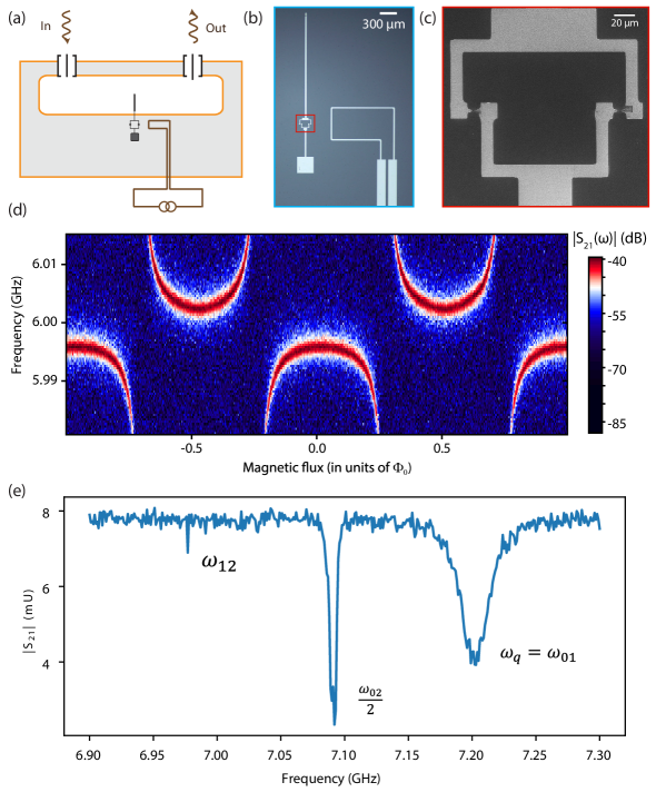
Figure 1: (a) A schematic of the device showing frequency tunable transmon qubit coupled to a 3D cavity. The SQUID loop is positioned in a small recess machined inside the cavity wall to incorporate a port for flux tuning. (b) An optical image of the sample showing the fabricated transmon qubit and the flux line. The thin vertical electrode provides the necessary qubit capacitance and couples to the fundamental mode of the 3D cavity. (c) Scanning electron microscope image of the SQUID loop. (d) Transmission through the cavity $|S_{21}|$ as the magnetic flux threaded by the SQUID loop is varied. (e) Qubit spectroscopy at the high drive power when qubit is flux biased at $\Phi=0$. Various qubit transitions are labeled accordingly. We determine the qubit anharmonicity to be $\approx$ 225 MHz.

Unlike the conventional 3D transmon the position of the SQUID loop is shifted away from the center of the cavity into a recess created in the cavity wall[35, 36]. As shown in Fig. 1(a), the SQUID is shifted to a recess designed inside the cavity wall. An antenna pointing towards the cavity center provides the necessary capacitance to the qubit mode and the coupling to the cavity mode. The transmon design was simulated using the black-box quantization technique [37]. Positioning the SQUID loop in a recess allows us to incorporate a local flux line near the SQUID loop to tune the qubit frequency rapidly. Such integration is also compatible with high coherence cavities designed from superconductors [27, 28, 38].

The flux control line is designed to avoid any perturbation to the cavity mode while minimizing the relaxation of qubit mode to the flux-drive port. Fig. 1(b) shows an optical microscope image of the fabricated device using the shadow evaporation technique on an intrinsic silicon substrate. Fig. 1(c) shows the scanning electron microscope image of the SQUID loop. The patterned device is placed inside an oxygen-free high thermal conductivity (OFHC) copper cavity and cooled down to 20 mK. Our measurement setup consists of various absorptive/reflective filters. Detailed schematic of the measurement setup is shown in the supplementary information (SI). We use a 1 GHz low-pass reflective filter on the flux-line and place it close to the flux drive port. The entire cavity assembly is placed inside the magnetic and infrared radiation shields.

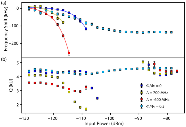
Figure 2: (a) Shift in the dressed cavity frequency as the input power to the cavity is increased for variable magnetic flux. The minimum power -129 dBm corresponds to the mean cavity occupation of 0.17 photons. The solid lines are numerical fits to extract the cavity nonlinearity. (b) The loaded (total) quality factor of the dressed mode for different input power to the cavity at multiple flux bias points.

We begin by performing spectroscopy measurements on the device. Fig. 1(d) shows the cavity spectroscopy measurement as the magnetic flux through the SQUID loop is changed by varying the current through the flux-line. An avoided crossing, signifying the strong coupling, between the qubit mode and the cavity mode is clearly visible. From the qubit spectroscopy, shown in Fig. 1(e), we determine the maximum qubit frequency (ground to first excited state transition) to be $\omega_{q}^{0}/2\pi\sim 7.203$ GHz and corresponding dressed cavity frequency for the ground state as $\omega_{c}/2\pi\sim 5.996$ GHz. We measure the coupling between two modes to be $g/2\pi\sim 87$ MHz, which is close to the designed value [37]. While the maximum qubit frequency depends on the total critical current of the two junctions, the minimum qubit frequency depends on the asymmetry of the two junctions. From the two-tone spectroscopy measurements, we could tracked the qubit frequency down to 4 GHz while tuning it with the flux. Various device parameters are summarized in Table 1.

At low probe power, the cavity frequency shifts to a dressed frequency due to its interaction with the qubit. Beyond a critical power, the cavity jumps to its bare frequency defining the dynamic range of the system. In this limit, the phase difference across the junctions evolves continuously. This has been attributed to the excitation of the qubit to the unconfined states lying outside the cosine potential well [25]. We use scqubits package to compute the energy eigen-states using the measured device parameters and find that there are approximately 10 confined states within the cosine potential well [39]. The higher transmon levels exhibit larger charge dispersion [40]. At large probe powers, the higher transmon levels become important, and the coupled system must be treated by including the Kerr-nonlinearity terms. In the dispersive limit, the Hamiltonian of the system can be written as $\hat{H}_{sys}/\hbar=\omega_{c}\hat{a}^{\dagger}\hat{a}+\omega_{q}\hat{b}^{\dagger}\hat{b}-\frac{1}{2}\alpha_{c}\hat{a}^{\dagger}\hat{a}^{\dagger}\hat{a}\hat{a}-\frac{1}{2}\alpha_{q}\hat{b}^{\dagger}\hat{b}^{\dagger}\hat{b}\hat{b}+\chi\hat{a}^{\dagger}\hat{a}\hat{b}^{\dagger}\hat{b}$, where $\omega_{c}$ ($\omega_{q}$) is the cavity (transmon) frequency, $\alpha_{c}$ ($\alpha_{q}$) is the cavity (transmon) Kerr-nonlinearity and $\chi$ is the dispersive shift. Due to the qubit-induced Kerr-nonlinearity, even in the dispersive regime the dynamic range of the cavity gets limited significantly. Fig. 2(a) shows the experimental results of the change in the dressed cavity frequency with probe power at the device. As the probe power is increased, the dressed cavity frequency changes as $\omega_{c}(\bar{n})=\omega_{c}(0)-2\alpha_{c}\bar{n}$ [11], where $\bar{n}$ is average number of photons in the cavity. From an independent calibration of $\bar{n}$ using ac-Stark shift, we deduce $\alpha_{c}$ for different qubit detunings. Additional dataset on ac-Stark shift is included in SI. For zero magnetic flux ($\Phi~{}=~{}0$), when qubit detuning $\Delta=\omega_{q}-\omega_{r}\approx 2\pi\times$1.2 GHz, we estimated the the cavity non-linearity to be $\alpha_{c}/2\pi=-3.2$ kHz. As the qubit mode is tuned closer to the cavity $\Delta=-2\pi\times$ 600 MHz, $\alpha_{c}/2\pi$ increases to $-27.8$ kHz, which is also indicated by the reduced dynamic range shown in the Fig. 2(a). As expected, the maximum dynamic range is achieved when the qubit is detuned furthest to the cavity frequency at $\Phi/\Phi_{0}=0.5$. At this flux-operating point, we also observe a reduction in the cavity frequency resulting from the asymmetry in the critical currents of the SQUID junctions. Similar behavior is observed in the corresponding quality factor of the dressed mode, as shown in the Fig. 2(b).

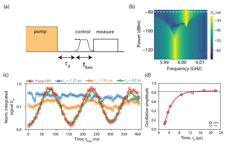
Figure 3: (a) A schematic of the pulse sequence used in the measurement. The cavity is driven with a strong pump pulse, which creates a large population of photons in the cavity and excites the transmon to unconfined states. Subsequently, Rabi measurement protocol with varying delays $\tau_{d}$ is followed. For control, we use a pulse that has a rise and fall parts defined by a gaussian function and central part of the pules is rectangular. The rise (and fall) part of the pulse is defined by a Gaussian function of length 35 ns and a $\sigma$ of 9 ns, indicated by the arrow. (b) Cavity transmission as probe power is increased while biasing the qubit at zero flux quantum. The white dotted line indicates the power used for the high power pulsed measurements. (c) Rabi measurement for different delays between the high power pump and qubit control pulse. A plot of Rabi oscillation without any high power pump is included as a reference. The pump power in the steady-state corresponds to a photon number $n_{d}$ of 2.1$\times 10^{4}$. (d) Amplitude of Rabi oscillation measured for different delays between the pump and the control pulse. Oscillation amplitude when the pump pulse is in off condition is denoted by the black dotted line. Statistical uncertainties from the fits are smaller than the marker size.

After the basic characterization of the device, we investigate the high power response in the time domain. The high pump power excites the qubit to unconfined states. It could be accompanied by the creation of quasi-particles, which could take a long time to relax. We perform time-domain measurements to probe the resurgence of coherence after subjecting the system to a strong pump.

Using the flux-bias, the qubit frequency is tuned to the maximum frequency $\Delta=\omega_{q}-\omega_{r}\approx 2\pi\times$1.2 GHz. A control pulse at the qubit frequency is applied. It is followed by a measurement pulse at the dressed cavity frequency, corresponding to a steady-state cavity occupation of $\approx$ 5 photons. The transmitted signal from the cavity is amplified at 4 K and at room temperature. The amplified signal is then down-converted to an intermediate frequency. Both quadratures of the IF signal are recorded as a function of time with a lock-in amplifier. To improve the readout signal contrast, we average fifty thousand time-traces of in-phase and quadrature streams of the readout signal.

Such an ensemble average of time traces can then be used to determine the qubit state. We follow an approach similar to Ref. [41] and define a normalized integrated signal $V_{H}$ as $V_{H}=\frac{1}{2}\frac{\sum_{i}\left(V_{g}(t_{i})-V_{m}(t_{i})\right)\Delta t}{\sum_{i}\left(V_{g}(t_{i})-V_{s}(t_{i})\right)\Delta t}$, where $\Delta t$ is the resolution of time-axis. $V_{g}$ ($V_{s}$) represents the averaged signal traces corresponding to the qubit in the ground state (in an equal mixture of ground and the first excited state). $V_{m}$ represents signal for the unknown qubit state that is being measured. Here, we effectively use the saturation control pulse for normalization. It is important to emphasize here that $V_{H}$ slightly deviates from the first excited state probability due to loss of population during the measurement process.

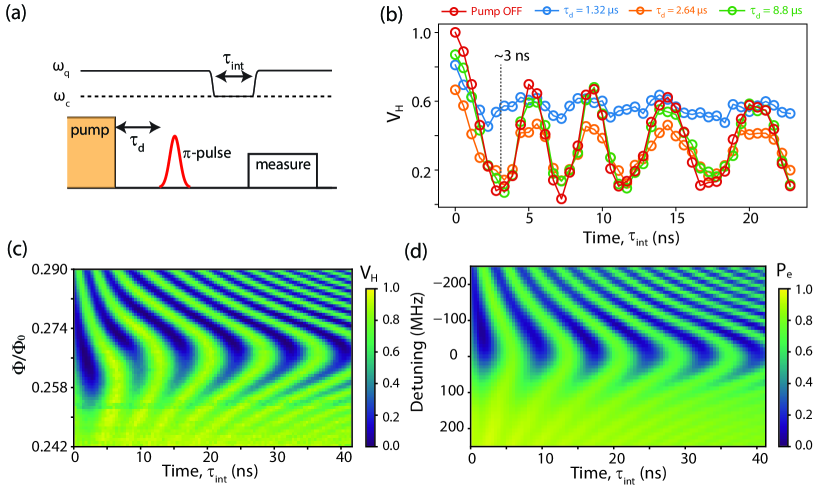
Figure 4: (a) A schematic of the pulse sequence used in the measurement. The interaction time ($\tau_{int}$) between cavity and qubit is varied for different values of $\tau_{d}$. (b) Normalized integrated signal showing the swap of excitation between the qubit and the cavity mode as the interaction length is varied. The black dotted line indicates the time to swap one excitation. (c) The colorplot of the normalized integrated signal as the detuning between the cavity mode and qubit is varied. The results were obtained from a different device with similar parameters. (d) The colorplot of the simulated qubit population in the excited state while varying the interaction length and relative detuning $\Delta=\omega_{q}-\omega_{c}$.

To probe the relaxation of qubit from the higher energy levels to the ground state, a strong pump tone is applied at the bare cavity frequency, followed by the pulsed control and readout scheme as described before. A schematic of the pulse sequence is shown in Fig. 3(a). In the presence of a strong pump, the transmon gets excited to the unconfined states resulting in the maximum transmission through the cavity at its bare frequency. Fig. 3(b) shows the measurement of transmission through the cavity as power of the probe signal is increased. The dressed mode shows the characteristic frequency shift due to the presence of the qubit. Beyond a critical power, the maximum transmission jumps to the bare cavity frequency. For the pump pulse, corresponding mean occupation of $n_{d}\sim$2.1$\times$10⁴ photons in the cavity indicated by the dotted line in Fig. 3(b). The calibration of the pump photons is performed by using the ac Stark measurements made at low probe powers. We have calibrated the total attenuation in the line and calculated the total number of photon with respect to bare cavity frequency. This strong pump pulse excites the qubit to higher unconfined states. By varying the length of the qubit control pulse, we perform the vacuum Rabi-oscillation measurement for different delay time ($\tau_{d}$) between the pump and qubit control.

Fig. 3(c) shows the measurements of normalized integrated signal $V_{H}$ for different delays. The horizontal axis corresponds to the duration of the qubit control pulse. For comparison, a measurement made in the absence of the pump pulse is included as well. For $\tau_{d}=$ 2.64 $\mu$s, we see small oscillations in the measurement indicating the coherent pouplation transfer between the ground and the first excited state. For such short delay time $\tau_{d}$, there are two effects that reduce the contrast of oscillations. First, the qubit population in the ground or first excited state could be low due to its excitation to higher levels. Second, for short times, the pump photon occupancy in the cavity can be substantial leading to dephasing. We use slowly varying control pulse and therefore rule out any leakage of qubit to the higher levels by the control pulse. For $\tau_{d}=$ 8.8 $\mu$s, the oscillations closely resemble the result obtained with pump maintained in off-condition. We systematically measure the amplitude of Rabi oscillations for different delay time between pump and the control pulse. Fig 3(d) shows the plot of oscillation amplitude for different delay times, showing the clear resurgence of the coherence in the device. Additional dataset is included in the SI. By fitting it to $\mathcal{F}(1-e^{\frac{t-t_{0}}{\tau}})$, we extract the characteristic timescale, $t_{0}+\tau\approx$ 4.8 $\mu$s for the relaxation from unconfined states. We point out here that such a timescale involves contributions from the relaxation of qubit from the higher excited states and from the dephasing due to occupancy of the cavity by pump-photons.

Device parameter	Symbol	Value
Bare cavity frequency	$\omega_{c}^{0}/2\pi$	6.002 GHz
Maximum qubit frequency	$\omega_{q}^{0}/2\pi$	7.203 GHz
Kerr-nonlinearity	$\alpha_{q}/2\pi$	$-225$ MHz
Maximum Joesphson energy	$E_{J}^{0}/h$	30.65 GHz
Cavity linewidth at zero flux	$\kappa/2\pi$	1.38 MHz
Qubit relaxation time at zero flux	$T_{1}$	2.11 $\mu$s
Qubit cavity coupling	$g/2\pi$	87 MHz

Table 1: Summary of device parameters studied in the main text

After characterizing the response of the device under high power, next, we perform the characterization of the flux bias port. We utilize the high bandwidth of the flux drive line and create a single-photon state in the cavity. The pulse protocol for such scheme is shown in Fig. 4(a). It consists of initializing the qubit to the first excited state by applying a $\pi$-pulse. The qubit frequency is then rapidly tuned to bring it in resonance with the cavity. The modes are maintained in resonance for a variable time $\tau_{int}$ and then the qubit mode is brought back to the original frequency followed by a measurement pulse. During the interaction period, the qubit and the cavity modes exchange the single excitation coherently. To understand the applicability of this scheme in a strongly driven system, we follow this protocol after a strong pump (at the bare cavity frequency) pulse with varied delay time $\tau_{d}$.

The current in the flux loop, controlling the qubit detuning, is applied using an arbitrary waveform generator. The shape of the flux-pulse is rectangular with rising and falling segments set as the half-gaussian with standard deviation of 1.1 ns. The width and the amplitude of the flux pulse are varied to control the interaction time and the qubit frequency, respectively. Fig. 4(b) shows $V_{H}$ as the interaction length is varied. For delay time of 8.8 $\mu$s ($>$ $t_{0}+\tau$), we observe that the qubit regains the coherence and oscillation due to the swapping of a single excitation can be clearly seen. Due to the strong coupling between the qubit and the cavity, it takes approximately 3 ns to transfer the single-photon from the qubit mode to the cavity mode indicated by the black dotted line.

Fig. 4(c) shows the colorplot of $V_{H}$ as the qubit detuning and interaction duration is varied. The oscillation frequency of the single excitation swap changes as the relative detuning between the qubit and cavity mode frequency is varied. At zero detuning, the oscillation frequency is minimum at 2$g$ and increases to $\sqrt{4g^{2}+\Delta^{2}}$ with detuning [13]. The deviation from the ideal chevron pattern suggests that the flux-pulse disperses as it travels down the sample. The initial change in the flux pulse is not able to tune the qubit in resonance with the cavity for short interaction time. We observe a small distortion in the chevron pattern for time-scales shorter than 10 ns. From this deviation, we concluded the bandwidth of the flux-line to be approximately 100 MHz. The bandwidth of flux line is limited by the parasitic capacitance and self-inductance of the current loop patterned near the SQUID loop. While we try to maintain a 50 $\Omega$ environment till the connector on the cavity, the impedance of the flux line on the silicon chip deviates from 50 $\Omega$ and this limits the bandwidth. Such distortions in flux-pulse, in principle, could be improved by using pre-compensated flux-pulses. To better understand the experimental results, we numerically simulate the system by solving the Lindblad master equation with the flux pulse sequence used in the experiment [42]. The simulated outcome of the excited state population is plotted in Fig. 4(d) with variable detuning in the vertical axis. The difference between the simulation and experimental plots can be understood from the distorted flux-pulse at the sample, as discussed above.

To summarize, we demonstrated a design of a fast-tunable transmon qubit in a 3D waveguide cavity architecture. We characterized its relaxation from unconfined states to the ground state after a high power drive pulse. We measure a resurgence time of 4.8 $\mu$s. We characterize the fast-flux line and find a bandwidth of $\approx$ 100 MHz. These performance benchmarking results provide the design guidelines for hybrid systems intended to integrate additional degrees of freedom with the circuit-QED platform [31, 32].

References

- [1] Castellanos-Beltran, M. A. and Lehnert, K. W. Applied Physics Letters 91(8), 083509 August (2007).
- [2] Yamamoto, T., Inomata, K., Watanabe, M., Matsuba, K., Miyazaki, T., Oliver, W. D., Nakamura, Y., and Tsai, J. S. Applied Physics Letters 93(4), 042510 July (2008).
- [3] Macklin, C., O’Brien, K., Hover, D., Schwartz, M. E., Bolkhovsky, V., Zhang, X., Oliver, W. D., and Siddiqi, I. Science 350(6258), 307–310 October (2015).
- [4] Devoret, M. H. and Martinis, J. M. Quantum Information Processing 3(1-5), 163–203 October (2004).
- [5] Blais, A., Gambetta, J., Wallraff, A., Schuster, D. I., Girvin, S. M., Devoret, M. H., and Schoelkopf, R. J. Physical Review A 75(3), 032329 March (2007).
- [6] Clerk, A. A., Lehnert, K. W., Bertet, P., Petta, J. R., and Nakamura, Y. Nature Physics 16(3), 257–267 (2020).
- [7] Buluta, I., Ashhab, S., and Nori, F. Reports on Progress in Physics 74(10), 104401 September (2011).
- [8] Xiang, Z.-L., Ashhab, S., You, J. Q., and Nori, F. Reviews of Modern Physics 85(2), 623–653 April (2013).
- [9] Flurin, E., Roch, N., Mallet, F., Devoret, M. H., and Huard, B. Physical Review Letters 109(18) October (2012).
- [10] Abdo, B., Sliwa, K., Schackert, F., Bergeal, N., Hatridge, M., Frunzio, L., Stone, A. D., and Devoret, M. Physical Review Letters 110(17), 173902 April (2013).
- [11] Leghtas, Z., Touzard, S., Pop, I. M., Kou, A., Vlastakis, B., Petrenko, A., Sliwa, K. M., Narla, A., Shankar, S., Hatridge, M. J., Reagor, M., Frunzio, L., Schoelkopf, R. J., Mirrahimi, M., and Devoret, M. H. Science 347(6224), 853–857 February (2015).
- [12] LaHaye, M. D., Suh, J., Echternach, P. M., Schwab, K. C., and Roukes, M. L. Nature 459(7249), 960–964 June (2009).
- [13] O’Connell, A. D., Hofheinz, M., Ansmann, M., Bialczak, R. C., Lenander, M., Lucero, E., Neeley, M., Sank, D., Wang, H., Weides, M., Wenner, J., Martinis, J. M., and Cleland, A. N. Nature 464(7289), 697–703 April (2010).
- [14] Lecocq, F., Teufel, J. D., Aumentado, J., and Simmonds, R. W. Nature Physics 11(8), 635–639 August (2015).
- [15] Pirkkalainen, J.-M., Cho, S. U., Li, J., Paraoanu, G. S., Hakonen, P. J., and Sillanpää, M. A. Nature 494(7436), 211–215 February (2013).
- [16] Zhu, X., Saito, S., Kemp, A., Kakuyanagi, K., Karimoto, S.-i., Nakano, H., Munro, W. J., Tokura, Y., Everitt, M. S., Nemoto, K., Kasu, M., Mizuochi, N., and Semba, K. Nature 478(7368) (2011).
- [17] Kubo, Y., Grezes, C., Dewes, A., Umeda, T., Isoya, J., Sumiya, H., Morishita, N., Abe, H., Onoda, S., Ohshima, T., Jacques, V., Dréau, A., Roch, J.-F., Diniz, I., Auffeves, A., Vion, D., Esteve, D., and Bertet, P. Physical Review Letters 107(22), 220501 (2011).
- [18] Gustafsson, M. V., Aref, T., Kockum, A. F., Ekström, M. K., Johansson, G., and Delsing, P. Science 346(6206), 207–211 (2014).
- [19] Manenti, R., Kockum, A. F., Patterson, A., Behrle, T., Rahamim, J., Tancredi, G., Nori, F., and Leek, P. J. Nature Communications 8(1), 975 (2017).
- [20] Bolgar, A. N., Zotova, J. I., Kirichenko, D. D., Besedin, I. S., Semenov, A. V., Shaikhaidarov, R. S., and Astafiev, O. V. Physical Review Letters 120(22), 223603 (2018).
- [21] Tabuchi, Y., Ishino, S., Noguchi, A., Ishikawa, T., Yamazaki, R., Usami, K., and Nakamura, Y. Science 349(6246), 405–408 July (2015).
- [22] Viennot, J., Ma, X., and Lehnert, K. Physical Review Letters 121(18), 183601 (2018).
- [23] Chu, Y., Kharel, P., Yoon, T., Frunzio, L., Rakich, P. T., and Schoelkopf, R. J. Nature 563(7733), 666 (2018).
- [24] Arrangoiz-Arriola, P., Wollack, E. A., Wang, Z., Pechal, M., Jiang, W., McKenna, T. P., Witmer, J. D., Van Laer, R., and Safavi-Naeini, A. H. Nature 571(7766), 537–540 (2019).
- [25] Lescanne, R., Verney, L., Ficheux, Q., Devoret, M. H., Huard, B., Mirrahimi, M., and Leghtas, Z. Physical Review Applied 11(1), 014030 (2019).
- [26] Verney, L., Lescanne, R., Devoret, M. H., Leghtas, Z., and Mirrahimi, M. Physical Review Applied 11(2), 024003 February (2019).
- [27] Gargiulo, O., Oleschko, S., Prat-Camps, J., Zanner, M., and Kirchmair, G. Applied Physics Letters 118(1), 012601 January (2021).
- [28] Reshitnyk, Y., Jerger, M., and Fedorov, A. EPJ Quantum Technology 3(1), 1–6 December (2016).
- [29] Yuan, M., Singh, V., Blanter, Y. M., and Steele, G. A. Nature Communications 6, 8491 October (2015).
- [30] Noguchi, A., Yamazaki, R., Ataka, M., Fujita, H., Tabuchi, Y., Ishikawa, T., Koji Usami, and Nakamura, Y. New Journal of Physics 18(10), 103036 (2016).
- [31] Gunupudi, B., Das, S. R., Navarathna, R., Sahu, S. K., Majumder, S., and Singh, V. Physical Review Applied 11(2), 024067 February (2019).
- [32] Peterson, G., Kotler, S., Lecocq, F., Cicak, K., Jin, X., Simmonds, R., Aumentado, J., and Teufel, J. Physical Review Letters 123(24), 247701 December (2019).
- [33] Ofek, N., Petrenko, A., Heeres, R., Reinhold, P., Leghtas, Z., Vlastakis, B., Liu, Y., Frunzio, L., Girvin, S. M., Jiang, L., Mirrahimi, M., Devoret, M. H., and Schoelkopf, R. J. Nature 536(7617), 441–445 August (2016).
- [34] Heeres, R. W., Reinhold, P., Ofek, N., Frunzio, L., Jiang, L., Devoret, M. H., and Schoelkopf, R. J. Nature Communications 8(1), 94 July (2017).
- [35] Paik, H., Schuster, D. I., Bishop, L. S., Kirchmair, G., Catelani, G., Sears, A. P., Johnson, B. R., Reagor, M. J., Frunzio, L., Glazman, L. I., Girvin, S. M., Devoret, M. H., and Schoelkopf, R. J. Physical Review Letters 107(24), 240501 December (2011).
- [36] Juliusson, K., Bernon, S., Zhou, X., Schmitt, V., le Sueur, H., Bertet, P., Vion, D., Mirrahimi, M., Rouchon, P., and Esteve, D. Physical Review A 94(6), 063861 December (2016). Publisher: American Physical Society.
- [37] Nigg, S. E., Paik, H., Vlastakis, B., Kirchmair, G., Shankar, S., Frunzio, L., Devoret, M. H., Schoelkopf, R. J., and Girvin, S. M. Physical Review Letters 108(24), 240502 June (2012).
- [38] Navau, C., Prat-Camps, J., Romero-Isart, O., Cirac, J., and Sanchez, A. Physical Review Letters 112(25), 253901 June (2014).
- [39] Groszkowski, P. and Koch, J. Quantum 5, 583 November (2021).
- [40] Koch, J., Yu, T. M., Gambetta, J., Houck, A. A., Schuster, D. I., Majer, J., Blais, A., Devoret, M. H., Girvin, S. M., and Schoelkopf, R. J. Physical Review A 76(4), 042319 October (2007).
- [41] Bianchetti, R., Filipp, S., Baur, M., Fink, J. M., Göppl, M., Leek, P. J., Steffen, L., Blais, A., and Wallraff, A. Physical Review A 80(4), 043840 October (2009).
- [42] Johansson, J. R., Nation, P. D., and Nori, F. Computer Physics Communications 183(8), 1760–1772 August (2012).