Abstract

Turbulence-free images cannot be produced by conventional computational ghost imaging because calculated light is not affected by the same atmospheric turbulence as real light. In this article, we first addressed this issue by measuring the photon number fluctuation autocorrelation of the signals generated by a conventional computational ghost imaging device. Our results illustrate how conventional computational ghost imaging without structural changes can be used to produce turbulence-free images.

1 Introduction

Ghost imaging with thermal light, in its most basic form, is an indirect imaging technique. Conventional ghost imaging requires two light beams: the reference beam, which never illuminates the object and is measured directly by a charged-coupled device (CCD), and the signal beam, which illuminates the object and is measured by a detector with no spatial resolution (bucket detector). The ghost image is restricted by a coincidence measurement of the signals from the two detectors. However, dual optical ghost imaging is not suitable for applications such as remote sensing [1,2], lidar sensing [3-5] and night vision [6-8]. Fortunately, Shapiro proposed computational ghost imaging in 2008 [9]. In this technique, the CCD detector is replaced with a virtual detector that calculates the propagation of the field of the reference beam. The image is reconstructed by correlating the calculated field patterns with the measured intensities at the object plane. As a result, computational ghost imaging, similar to classical optical imaging, only has one optical path, which has attracted increasing attention [1,6,7,10-13].

Although ghost imaging technology has many advantages, such as superresolution [14] and indirect imaging capabilities [15,16], its most valuable property is its incredible turbulence-free imaging capability. This practical property is an important milestone for optical imaging because any fluctuation index disturbance introduced in the optical path will not affect the image quality [17-19]. However, previous research has shown that turbulence-free imaging has certain conditions that must be met [20,21]. One of the critical conditions is that two optical paths need to pass through the same turbulence. For computational ghost imaging, there is only one optical path. This optical path is affected by atmospheric turbulence, while the other virtual optical path is obtained through calculation. Thus, these two optical paths cannot be affected by the same atmospheric turbulence. Thus, turbulence-free images cannot be obtained from conventional computational ghost imaging [19]. Although some methods, such as adaptive optics and depth learning, have significantly improved the image quality of computational ghost imaging in turbulent environments, these methods are difficult to produce a turbulence-free image [22-24].

To solve this challenging problem, we used a conventional computational ghost imaging device as a signal acquisition terminal. The signals produced by this device were duplicated into two identical copies. Thus, both sets of data were affected by the same atmospheric turbulence. As a result, turbulence-free images were produced. Finally, the turbulence-free image was restructured by measuring the photon number fluctuation autocorrelation of the two signals.

2 Theory

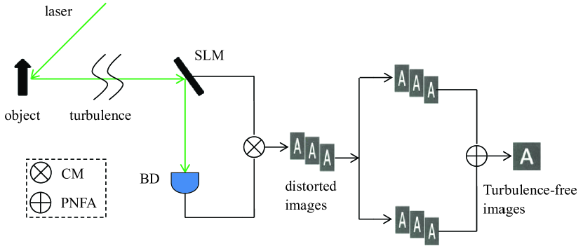
Fig. 1: (a) Setup for turbulence-free computational ghost imaging. SLM: spatial light modulator, BD: bucket detector. CM: coincidence measurement, PNFA: photon number fluctuation autocorrelation.

The setup for turbulence-free computational ghost imaging is illustrated in Fig. 1. A laser beam illuminated an object $T(x)$; then, the reflected light that passed through atmospheric turbulence was received and modulated by a spatial light modulator (SLM). The light intensity was detected by a bucket detector and can be expressed as $\sum_{p}E\left(x,t\right)T\left(x\right)e^{i\phi}$, where $p$ represents $p$th subfield from the $p$th subsource, $e^{i\phi}$ represents the atmospheric turbulence factor [17,18,22-26]. Because the calculated light is based on the input signal of the SLM, it is not affected by atmospheric turbulence [9,23,24,27]. Thus, the calculated light can be expressed as $\sum_{q}E\left(x,t\right)$, where $q$ represents $q$th subfield from the $q$th subsource. The signal produced by the conventional computational ghost imaging device can be expressed as [9,17,21,24,25]

$$C\left(x,x^{{}^{\prime}}\right)=\left\langle\sum_{p}\left|E\left(x,t\right)T\left(x\right)e^{i\phi}\right|^{2}\sum_{q}\left|E\left(x,t\right)\right|^{2}\right\rangle-\left\langle\sum_{p}\left|E\left(x,t\right)T\left(x\right)e^{i\phi}\right|^{2}\right\rangle\left\langle\sum_{q}\left|E\left(x,t\right)\right|^{2}\right\rangle.$$ (1)

Equation (1) shows that turbulence-free images cannot be reconstructed by computational ghost imaging because the calculated light $\sum_{q}E\left(x,t\right)$ is not affected by the same atmospheric turbulence as the real light $\sum_{p}E\left(x,t\right)T\left(x\right)e^{i\phi}$.

To solve this problem, we duplicated the signal produced by the conventional computational ghost imaging device into two identical copies. Thus, both sets of data were affected by the same atmospheric turbulence. As a result, the conditions for turbulence-free imaging were met. Then, turbulence-free images were obtained by analysing both data sets based on the photon number fluctuation autocorrelation. It was assumed that one image was generated for every $m$ measurements. Thus, after $m\times n$ measurements, $n$ images were produced. These $n$ images were duplicated (see the data processing section in Fig. 1). The photon number fluctuation autocorrelation algorithm was used to process these two data sets. The autocorrelation algorithm for the photon number fluctuation is described below. The software first calculated the average number of counts in a short time window $\overline{C}$. Two virtual logic circuits (post-neg identifiers) classified the number of counts per window as positive or negative fluctuations based on $\overline{C}$. Thus, we have

$$\Delta C_{\alpha}^{(+)} =\left\{\begin{array}[]{c}C_{\alpha}-\overline{C},if,C_{\alpha}>\overline{C}\\ 0,otherwise\end{array}\right.$$ (4)

$$\Delta C_{\alpha}^{(-)} =\left\{\begin{array}[]{c}C_{\alpha}-\overline{C},if,C_{\alpha}<\overline{C}\\ 0,otherwise,\end{array}\right.$$ (7)

where $\alpha=1$ to $n$ is used to label the $\alpha$th short time window, $\Delta C$ is the photon number fluctuation. Then, we defined the following quantities for the statistical correlation calculations:

$$\left(\Delta C\Delta C^{\prime}\right)_{\alpha}^{\left(++\right)} =\left|\Delta C_{\alpha}^{(+)}\Delta C_{\alpha}^{{}^{\prime}(+)}\right|,$$

$$\left(\Delta C\Delta C^{\prime}\right)_{\alpha}^{\left(--\right)} =\left|\Delta C_{\alpha}^{(-)}\Delta C_{\alpha}^{{}^{\prime}(-)}\right|,$$

$$\left(\Delta C\Delta C^{{}^{\prime}}\right)_{\alpha}^{\left(+-\right)} =\left|\left(\overline{C}-\Delta C_{\alpha}^{(+)}\right)\left(\overline{C}-\Delta C_{\alpha}^{{}^{\prime}(-)}\right)\right|,$$

$$\left(\Delta C\Delta C^{{}^{\prime}}\right)_{\alpha}^{\left(-+\right)} =\left|\left(\overline{C}-\Delta C_{\alpha}^{(-)}\right)\left(\overline{C}-\Delta C_{\alpha}^{{}^{\prime}(+)}\right)\right|.$$ (8)

The statistical fluctuation-fluctuation correlation $\left\langle\Delta C\Delta C^{{}^{\prime}}\right\rangle$ is then calculated from

$$\left\langle\Delta C\Delta C^{{}^{\prime}}\right\rangle=\frac{1}{n}\left[\sum_{\alpha=1}^{n}\left(\Delta C\Delta C^{{}^{\prime}}\right)_{\alpha}^{\left(++\right)}+\sum_{\alpha=1}^{n}\left(\Delta C\Delta C^{{}^{\prime}}\right)_{\alpha}^{\left(--\right)}\right.$$

$$+\left.\sum_{\alpha=1}^{n}\left(\Delta C\Delta C^{{}^{\prime}}\right)_{\alpha}^{\left(+-\right)}+\sum_{\alpha=1}^{n}\left(\Delta C\Delta C^{{}^{\prime}}\right)_{\alpha}^{\left(-+\right)}\right].$$ (9)

We have [28-30]

$$\left\langle\Delta C\Delta C^{{}^{\prime}}\right\rangle\propto\sum_{p\neq q}\left|E_{p}^{{}^{\ast}}\left(x,t\right)E_{q}\left(x^{{}^{\prime}},t\right)E_{q}\left(x^{{}^{\prime}},t\right)E_{p}^{{}^{\ast}}\left(x,t\right)T^{2}\left(x\right)\right|^{2}e^{i2\left(\phi+\phi^{{}^{\prime}}\right)}$$ (10)

At $x=x^{{}^{\prime}}$, $e^{i2\left(\phi+\phi^{{}^{\prime}}\right)}=1$, and the cross-interference term reaches its turbulence-free constructive maximum.

3 Experiments and results

The experimental setup was a conventional computational ghost imaging setup, except for the data processing part. A semiconductor laser beam ($\lambda=$532 nm, 30 mW, Changchun New Industries Optoelectronics Technology Co., Ltd. MGL-III-532) was used to illuminate a two-dimensional amplitude-only ferroelectric liquid crystal SLM (FLC-SLM, Meadowlark Optics A512-450-850), which had 512$\times$512 addressable 15$\mu m\times$15$\mu m$ pixels. Then, the modulated light illuminated the object. Finally, the reflected light, which carried information about the object, was collected by a bucket detector. In this experiment, atmospheric turbulence was introduced by adding conventional heating elements below certain sections of the optical path. Heating the air causes temporal and spatial fluctuations in the index of refraction, causing the traditional image of the object to jitter randomly in the image plane and become distorted. The length of the heating element was 0.4 m. The heating temperature was approximately 220^∘C. The photon number fluctuation autocorrelation algorithm was written in MATLAB 2014a.

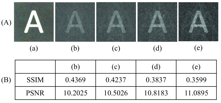
Fig. 2: (A) (a) The object and (b-e) the reconstructed images for different measurements. (b) $m=500$, $n=20$, (c) $m=1000$, $n=10$, (d) $m=2000$, $n=5$, (e) $m=5000$, $n=2$. (B) The SSIM and PSNR values of the reconstructed images.

We assumed that the computational ghost imaging device generated an image every $m$ measurements. After $m\times n$ measurements, $n$ images were produced. The first experimental results demonstrated that the images reconstructed by our method were related to both $m$ and $n$. Fig. 2 clearly shows that when $m\times n=10000$, the greater $m$ is, the brighter the reconstructed image, but the lower the image quality. We used the structural similarity (SSIM) index and the peak signal-to-noise ratio (PSNR) to quantitatively measure the imaging quality of this method and conventional computational ghost imaging [24].

Fig. 3: Top row: the reconstructed images obtained by computational ghost imaging with different measurements. (a1-a4) 1000, 4000, 7000, 10000. Bottom row: the reconstructed images obtained by our method. (b1)$m=500,n=2$, (b1)$m=500,n=8$, (b1)$m=500,n=14$, (b1)$m=500,n=20$.

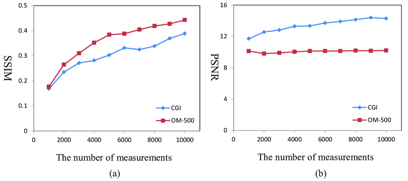
Fig. 4: The (a) SSIM and (b) PSNR curves of the images reconstructed by computational ghost imaging and our method, respectively. CGI: computational ghost imaging, OM-500: our method with $m=500$.

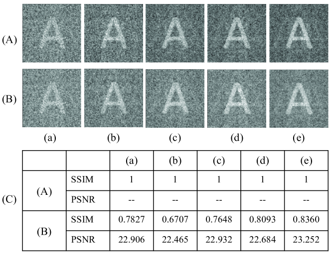
Fig. 5: (A) Computational ghost images without atmospheric turbulence. (B) Distorted images affected by atmospheric turbulence. (a-e) Measurement times of 1000, 2000, 3000, 4000 and 5000, respectively. (C) The SSIM and PSNR values of the images corresponding to the above figures.

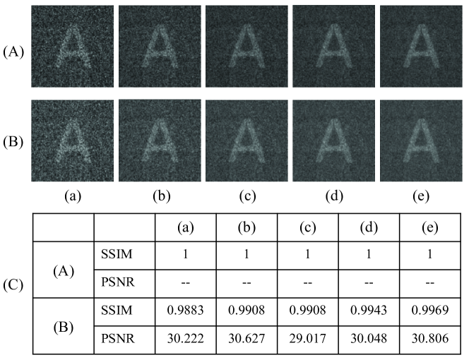
Fig. 6: (A) Images reconstructed by our method without atmospheric turbulence. (B) Images reconstructed by our method with atmospheric turbulence. (a-e) Measurement times of 1000, 2000, 3000, 4000 and 5000, respectively, with $m=500$. (C) The SSIM and PSNR values of the images corresponding to the above figures.

In the second experiment, we compared the quality of images reconstructed by conventional computational ghost imaging and this method. Figure 3 shows that the background noise of images reconstructed by this method was lower than that of images reconstructed by conventional computational ghost imaging. Moreover, Fig. 3 shows that the quality of the reconstructed images improved as the measurement time increased. Fig. 4 shows that for the same number of measurements, the quality of the images reconstructed by our method was higher than that of the images reconstructed by conventional computational ghost imaging (SSIM index), but the image brightness (PSNR index) was lower than that of computational computational ghost imaging.

In the third experiment, we demonstrated that this method produced turbulence-free images. The effect of turbulence on conventional computational ghost imaging is shown in Fig. 5, while the results reconstructed by our method are shown in Fig. 6. Fig. 5A shows a typical result of computational ghost imaging in the absence of atmospheric turbulence, while Fig. 5B shows the result of computational ghost imaging with atmospheric turbulence. Figure 5C shows a quantitative comparison. Here, we used the computational ghost images without atmospheric turbulence as reference images. Similarly, Fig. 6A shows the result of our method without atmospheric turbulence, while Fig. 6B shows the corresponding result with atmospheric turbulence. Considering the fluctuation of light source, it is clear that the images reconstructed by our method are turbulence-free images.

4 Conclusion

These experiments demonstrate turbulence-free computational ghost imaging. The problem that the calculated light differs from the actual light affected by turbulence can be solved by measuring the photon number fluctuation autocorrelation of the signal generated by a computational ghost imaging device. Moreover, the quality of the images reconstructed by this method was related not only to the total amount of data, but the number of images generated by the computational ghost imaging device. When the sampling amount is fixed, the fewer measurements per image produced by the computational ghost imaging device, the better the overall result. We hope that this method can provide a promising solution to overcome issues with atmospheric turbulence in remote sensing and lidar applications.

This work was supported by the National Natural Science Foundation of China (11704221,11574178, 61675115); Taishan Scholar Foundation of Shandong Province (tsqn201812059).

Disclosures: The authors declare no constricts of interest.

Data Availability Statement: Data underlying the results presented in this paper are not publicly available at this time but may be obtained from the authors upon reasonable request.

References

- [1] B. I. Erkmen, Computational ghost imaging for remote sensing, J. Opt. Soc. Am. A 29, 782–789 (2012).
- [2] C. Zhang, W. Gong, and S. Han, Ghost imaging for moving targets and its application in remote sensing, Chin. J. Lasers 39, 1214003 (2012).
- [3] C. Zhao, W. Gong, M. Chen, E. Li, H. Wang, W. Xu, and S. Han, Ghost imaging lidar via sparsity constraints, Appl. Phys. Lett. 101, 141123 (2012).
- [4] N. D. Hardy and J. H. Shapiro, Computational ghost imaging versus imaging laser radar for three-dimensional imaging, Phys. Rev. A 87, 023820 (2013).
- [5] W. L. Gong, C. Q. Zhao, H. Yu, M. L. Chen, W. D. Xu, and S. S. Han, Three-dimensional ghost imaging lidar via sparsity constraint, Sci. Rep 6, 26133 (2016).
- [6] H. C. Liu and S. Zhang, Computational ghost imaging of hot objects in long-wave infrared range, Appl. Phys. Lett. 111, 031110 (2017).
- [7] D. Y. Duan and Y. J. Xia, Pseudo color night vision correlated imaging without an infrared focal plane array, Opt. Express 29, 4978–4985 (2021).
- [8] D. Y. Duan, R. Zhu, and Y. J. Xia, Color night vision ghost imaging based on a wavelet transform, Opt. Lett. 46, 4172–4175 (2021).
- [9] J. H. Shapiro, Computational ghost imaging, Phys. Rev. A 78, 061802(R) (2008).
- [10] M. Le, G. Wang, H. Zheng, J. Liu, Y. Zhou, , and Z. Xu, Underwater computational ghost imaging, Opt. Express 25, 22859–22868 (2017).
- [11] Z. Xu, W. Chen, J. Penuelas, M. Padgett, and M. Sun, 1000 fps computational ghost imaging using ledbased structured illumination, Opt. Express 26, 2427–2434 (2018).
- [12] F. Wang, H. Wang, H. Wang, G. Li, and G. Situ, Learning from simulation: An end-to-end deep-learning approach for computational ghost imaging, Opt. Express 27, 25560–25572 (2019).
- [13] S. Rizvi, J. Cao, K. Zhang, and Q. Hao, Deepghost: realtime computational ghost imaging via deep learning, Sci. Rep 10, 11400 (2020).
- [14] W. Li, Z. Tong, K. Xiao, Z. Liu, Q. Gao, J. Sun, S. Liu, S. Han, and Z. Wang, Single-frame wide-feld nonoscopy based on ghost imaging via sparsity constraints, Optica 6, 1515–1523 (2019).
- [15] F. Wang, C. Wang, M. Chen, W. Gong, Y. Zhang, S. Han, and G. Situ, Far-field super-resolution ghost imaging with a deep neural network constraint, Light. Sci. Appl. 11, 1 (2022).
- [16] J. H. Shapiro and R. W. Boyd, The physics of ghost imaging, Quantum Inf. Process. 11, 949–993 (2012).
- [17] R. E. Meyers, K. S. Deacon, and Y. Shih, Turbulence-free ghost imaging, Appl. Phys. Lett. 98, 111115 (2011).
- [18] R. E. Meyers, K. S. Deacon, and Y. H. Shi, Positive negative turbulence-free ghost imaging, Appl. Phys. Lett. 100, 131114 (2012).
- [19] Y. H. Shih, An Introduction to Quantum Optics: Photon and Biphoton Physics (Series in Optics and Optoelectronics) (Taylor & Francis, 2011).
- [20] J. H. Shapiro, Comment on turbulence-free ghost imaging [appl. phys. lett. 98, 111115 (2011)], arXiv 1201.4513 (2012).
- [21] M. F. Li, L. Yan, R. Yang, J. Kou, and Y. S. Liu, Turbulence-free intensity fluctuation self-correlation imaging with sunlight, Acta Phys. Sin. 68, 094204 (2019).
- [22] D. Shi, C. Fan, P. Zhang, J. Zhang, H. Shen, C. Qiao, and Y. Wang, Adaptive optical ghost imaging through atmospheric turbulence, Opt. Express 20, 27992–27998 (2012).
- [23] Y. Zhao, B. Dong, M. Liu, Z. Zhou, and J. Zhou, Deep learning based computational ghost imaging alleviating the effects of atmospheric turbulence, Acta Opt. Sin. 41, 1111001 (2021).
- [24] H. Zhang and D. Duan, Turbulence-immune computational ghost imaging based on a multi-scale generative adversarial network, Opt. Express 29, 43929–43937 (2021).
- [25] J. Cheng, Ghost imaging through turbulent atmosphere, Opt. Express 17, 7916–7921 (2009).
- [26] J. Cheng and J. Lin, Unified theory of thermal ghost imaging and ghost diffraction through turbulent atmosphere, Phys. Rev. A 87, 043810 (2013).
- [27] Y. Bromberg, O. Katz, and Y. Silberberg, Ghost imaging with a single detector, Phys. Rev. A 79, 053840 (2009).
- [28] H.Chen, T. Peng, and Y. Shih, 100% correlation of chaotic thermal light, Phys. Rev. A 88, 023808 (2013).
- [29] Y. H. Shih, The physics of turbulence-free ghost imaging, Technologies 4, 39 (2016).
- [30] D. Duan and Y. Xia, Can a conventional optical camera realize turbulence-free imaging? arXiv 2109:03995 (2021).