Nanometer-Scale Nuclear Magnetic Resonance Diffraction with Sub-Ångstrom Precision

Abstract

Achieving atomic resolution is the ultimate limit of magnetic resonance imaging (MRI), and attaining this capability offers enormous technological and scientific opportunities, from drug development to understanding the dynamics in interacting quantum systems. In this work, we present a new approach to nanoMRI utilizing nuclear magnetic resonance diffraction (NMRd) — a method that extends NMR imaging to probe the structure of periodic spin systems. The realization of NMRd on the atomic scale would create a powerful new methodology for materials characterization utilizing the spectroscopic capabilities of NMR. We describe two experiments that realize NMRd measurement of ³¹P spins in an indium-phosphide (InP) nanowire with sub-Ångstrom precision. In the first experiment, we encode a nanometer-scale spatial modulation of the $z$-axis magnetization by periodically inverting the ³¹P spins, and detect the period and position of the modulation with a precision of $<0.8~{}\text{\AA}$. In the second experiment, we demonstrate an interferometric technique, utilizing NMRd, for detecting an Ångstrom-scale displacement of the InP sample with a precision of 0.07 Å. The diffraction-based techniques developed in this work represent new measurement modalities in NMR for probing the structure and dynamics of spins on sub-Ångstrom length scales, and demonstrate the feasibility of crystallographic MRI measurements.

I Introduction

Three-dimensional atomic-resolution nuclear magnetic resonance (NMR) imaging of nanometer scale materials remains a long-standing challenge. The ability to image biologically-relevant structures such as proteins and virus particles on the atomic scale with the spectroscopic capabilities of NMR would fundamentally advance our understanding of their function, and potentially lead to new drug therapies [1, 2, 3]. In addition, atomic-scale magnetic resonance imaging (MRI) could be a powerful tool for studying magnetic correlations in condensed matter systems [4]. Over the past two decades, significant advances have been made to extend the capabilities of MRI to the nanometer and Ångstrom scales [5, 6, 7, 8, 9, 10, 11, 12, 13, 14, 15, 16], including the detection of single sub-surface electron spins [5, 6], MRI of single atoms on a surface [7], NMR detection of single proteins [8], three-dimensional imaging of individual tobacco-mosaic virus particles [9], and the detection and coherent control of individual carbon spins in diamond [10] with sub-Ångstrom resolution [11].

Many of these approaches rely on the use of local probes to directly detect the distribution of spins within the sample. While such techniques are well-suited for imaging arbitrary spin distributions, scattering techniques that employ coherent sources, e.g., X-rays, neutrons or electrons, offer an alternative means of determining the atomic-scale structure of crystalline materials that possess a high degree of spatial correlation. Unlike direct-space techniques that locally probe the material density, scattering techniques rely on the interference of the scattered field from each scattering center within the detection volume, providing a highly efficient means of structure determination.

MRI, like X-ray and neutron scattering, is a reciprocal space technique, in which the measured signal $s(\mathbf{k})\sim\int\rho(\mathbf{r})\,e^{i\mathbf{k}\cdot\mathbf{r}}\,d^{3}r$ is proportional to the Fourier transform of the matter density. This similarity with scattering led Mansfield and Grannell in 1973 to propose NMR ‘diffraction’ (NMRd), as a method for determining the lattice structure of crystalline materials [17]. The realization of crystallographic NMRd would extend the spectroscopic capabilities of MRI to the atomic scale and provide a fundamentally new non-destructive method for measuring the structure factor of crystalline materials. Furthermore, being a phase-sensitive technique, NMRd would permit real-space reconstruction of the spin density, without the loss of phase information common to scattering techniques, such as X-rays, that measure the scattered field intensity.

The main challenge to achieving atomic scale NMRd lies in the difficulty of making the encoding wavenumber $k$ sufficiently large . For example, the largest encoding wavenumbers achieved in clinical high-resolution MRI scanners are of order $k/(2\pi)\sim 10^{4}\,\text{m}^{-1}$, which is more than a factor of $10^{5}$ smaller than what is needed to measure typical atomic spacings [19]. In the past two decades, the principal technologies needed to overcome this challenge have been developed in the context of force-detected nanoMRI, paving the way for realizing atomic-scale NMRd, which would establish a new modality for materials characterization and imaging.

In this work, we present two experiments that utilize key advances in nanoMRI technology — namely the ability to generate large time-dependent magnetic field gradients, and the ability to detect and coherently control nanoscale ensembles of nuclear spins — to generate encoding wavenumbers as large as $k/(2\pi)=0.48\ \text{\AA}^{-1}$ and realize NMRd measurements of ³¹P spins of an indium phosphide (InP) sample with sub-Ångstrom precision. These results represent a significant step towards extending the spectroscopic and phase-sensitive imaging capabilities of MRI to atomic-scale materials characterization.

In the first experiment, we demonstrate phase-sensitive NMRd detection by encoding a ‘diffraction grating’ via periodic modulation of the ³¹P $z$-axis magnetization, with a mean period of 4.5 nm in a $(\sim 50~{}\text{nm})^{3}$ volume, and detect the position and period of the grating with a precision of $<0.8~{}\text{\AA}$. In the second experiment, we present a method for interferometric displacement detection using NMRd, which we apply to measure an Ångstrom-scale displacement of the InP sample with a precision of 0.07 Å.

II NMRd Concept

To illustrate the basic concept of NMRd as envisioned in Ref. [17], we consider a one-dimensional spin density having a spatially periodic modulation—such as a linear spin chain with spacing $a$ as shown in Fig. 1—that evolves in a uniform field gradient $G_{x}=\partial B/\partial x$ for a time $\tau_{e}$. The wavevector corresponding to the helical winding encoded in the spins is $k_{x}=\gamma\,G_{x}\,\tau_{e}$, where $\gamma$ is the spin gyromagnetic ratio. At particular encoding times $\tau_{\text{echo}}=2\pi n/(\gamma\,G_{x}\,a)$, corresponding to $k_{x}a=2\pi n$, the relative phase between neighboring spins becomes $\Delta\varphi=2\pi n$, $n\in\{1,2,3,\dots\}$ and a ‘diffraction echo’ (DE) is observed. At the peak of the echo, the signal from each spin adds constructively, in exact analogy to the diffraction peak observed in a scattering experiment. The lattice constant is determined from the location of the DE peak, and the shape of the sample from the Fourier transform of the DE envelope. Because the encoding wavevector is spin selective, the structure factor corresponding to each NMR-active nucleus can be determined separately. The NMRd concept illustrated in Fig. 1 can be readily generalized to three dimensions, with $\mathbf{k}=\gamma\mathbf{G}\tau_{e}$ and $\mathbf{G}=\gradient B$, where $B$ represents the magnitude of either the static or the radio frequency (RF) field at the Larmor frequency, used for phase encoding. The diffraction condition in three dimensions corresponds to $\mathbf{k}\cdot\mathbf{a}_{j}=2\pi n$, where $\mathbf{a}_{j}$ are the primitive vectors of the lattice.

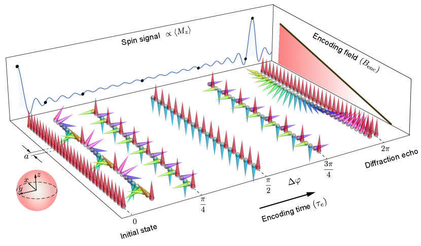
Figure 1: Time evolution of a one-dimensional periodic lattice of spins, starting from a uniform $z$ state at $\tau_{e}=0$, under a linearly varying external field along the lattice. The $x,y,z$ coordinate axes on the left marks the Bloch sphere directions for the spins represented by the cones. For $\tau_{e}>0$, the spins dephase and the expectation value of the $z$-axis magnetization $\expectationvalue{M_{z}}$ drops to zero. Once the spins on adjacent lattice sites complete a full rotation $(\Delta\varphi=2\pi)$, the spins rephase and a diffraction echo in $\expectationvalue{M_{z}}$ appears.

Being particularly sensitive to hydrogen atoms, NMRd could enable structural characterization of nanocrystalline organic solids via NMR. For example, a lattice of ¹H spins with $a=3~{}\text{\AA}$ evolving under a uniform field gradient of $10^{5}$ T/m would produce a DE at $\tau_{e}=780~{}\mu\text{s}$. While the dephasing times in most organic solids are much shorter, typically of order $T_{2}\sim 20~{}\mu\text{s}$, dynamical decoupling NMR pulse sequences, such as the symmetric magic echo sequence [20], can be used to extend the coherence time into the millisecond range, while allowing for encoding with both static and resonant RF field gradient pulses. Importantly, although the concept of NMRd was first envisioned as a technique to study crystal structures, it can be applied more broadly to probe any spatially-periodic spin-state modulation, e.g., a periodic modulation of the $z$-axis magnetization, that can be refocused by the evolution under the field gradient. It can therefore also be used to study quantum transport of periodic spin systems on atomic length scales.

III Experimental Setup

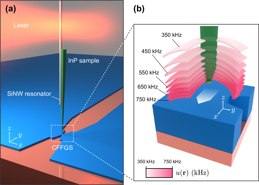
Figure 2: (a) Schematic of the experimental setup, including the SiNW force sensor, the current-focusing field-gradient source (CFFGS), and the InP spin sample. During spin detection, 70-mA peak current was applied to the CFFGS at the resonance frequency of the SiNW, which produced a time-dependent field gradient with a peak amplitude of $\partial B_{z}/\partial y=$ 8 G/nm, 50 nm above the surface. The Rabi field $B_{1}(\mathbf{r})=\sqrt{B_{x}^{2}(\mathbf{r})+B_{y}^{2}(\mathbf{r})}/2$ used for NMR was produced by driving the CFFGS with 70 mA-pk currents at the resonance frequency of ³¹P spins, which produced a $B_{1}$ field with an amplitude of 470 G, and a $B_{1}$ field gradient of $\partial B_{1}/\partial z=-4$ G/nm, 50 nm above the surface. Further details regarding the field profile produced by the CFFGS are provided in Sec. II of Ref. [21]. (b) Simulated contours of constant Rabi frequency $u(\mathbf{r})=\gamma B_{1}(\mathbf{r})/(2\pi)$, where $\gamma=2\pi\times 17.235$ MHz/T is the ³¹P gyromagnetic ratio. The contours within the sample are nearly parallel to the $xy$ plane and vary primarily in the $z$ direction.

Force-detected magnetic resonance measurements were performed using a silicon nanowire (SiNW) mechanical resonator, which served as the mechanical sensor to detect the force exerted on ³¹P spins in an InP nanowire (InPNW) placed in a magnetic field gradient. The experimental setup, shown in Fig. 2(a), is similar to the one used in our previous nanoMRI work [16]. The SiNW was grown via the vapor-liquid-solid method near the edge of a $1.5~{}\text{mm}\times 1~{}\text{mm}\times 0.4~{}\text{mm}$ Si(111) substrate, and had a length of 20 $\mu$m, and a 100 nm diameter [22]. The frequency of the fundamental flexural mode of the as-grown SiNW was approximately 250 kHz prior to sample attachment, and had a spring constant of 0.6 mN/m. Experiments were carried out at a base temperature of 4 K in high vacuum. At this temperature, the quality factor of the SiNW was approximately 60,000. The SiNW chip was glued to a millimeter size piezoelectric transducer (PT), which was used to apply various control signals to the SiNW. To increase the measurement bandwidth of the resonator, a feedback signal was applied to the PT, which reduced the quality factor of the SiNW to 700 [23].

The InPNW sample used in this work was approximately 5-$\mu$m long, with $\sim 100$-nm diameter, grown with a Wurtzite structure [24]. The sample was attached $\sim 3-4$ $\mu$m away from the tip of the SiNW, with the axes of the two nanowires aligned parallel to each other, and the tip of the InPNW extending $\sim 2\,\mu\text{m}$ beyond the tip of the SiNW. Details of the attachment procedure are provided in Sec. I of Ref. [21]. A video of the sample attachment is also included in [21]. After sample attachment, the resonance frequency of the SiNW decreased to 163 kHz, however no significant change in the quality factor was observed.

NMR measurements were performed by applying a static field of $B_{0}=3$ T parallel to the the InPNW axis. At this field, the Larmor frequency of the ³¹P spins is $\omega_{0}/(2\pi)=51.7\,\text{MHz}$. To generate time-varying magnetic fields and magnetic field gradients used for spin measurements, we fabricated a current focusing field gradient source (CFFGS) by electron-beam lithography and reactive ion-beam etching of a 100-nm thick Al film deposited on a sapphire substrate. The device contained a 150-nm-wide and 50-nm-long constriction, which served to focus electrical currents to produce the magnetic fields used for spin detection and control. All measurements were carried out with the tip of the InPNW placed at the center of the CFFGS and positioned $\sim 50$ nm above the surface.

IV Nanometer-Scale NMRd Measurements

To observe a focused diffraction echo – i.e., one in which the spectral weight of the echo is localized within a narrow range of encoding times – the spin-state modulation must be a periodic function of the encoding field coordinate, e.g., for a spin density with a spatially periodic modulation, the encoding field profile must vary linearly in space (Fig. 1). As a demonstration of nanometer scale NMRd, we utilize the Rabi-field gradient to (1) create a diffraction grating by periodically inverting the $z$-axis magnetization of the ³¹P spins within the measured volume of the InP tip [Fig. 3(a)], and (2) generate the encoding wavevector for the NMRd measurements. In so doing, we ensure that the spin modulation is a periodic function of the encoding field.

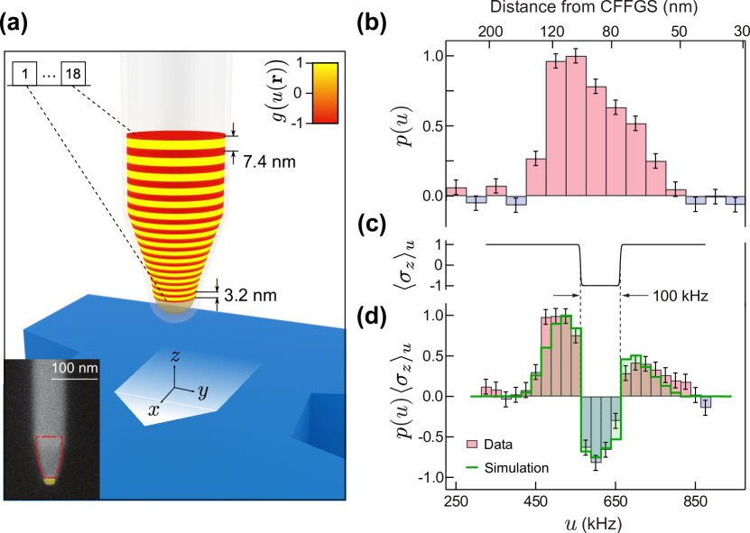
Figure 3: (a) Spatial configuration of the InP spin sample brought 50 nm above the surface of the CFFGS device. The CFFGS surface lies perpendicular to the static external magnetic field $B_{0}~{}\hat{\mathbf{z}}$. The 18 regions indicated in red represent the regions inverted by the band-inversion pulses within $g(u)$. (Inset) Scanning electron microscope (SEM) image of a representative InPNW. The measured volume of the sample is indicated by the outlined region. (b) Measured Rabi-frequency distribution $p(u)$ of the ³¹P spins in the detection volume shown in (a). The data was obtained by sampling 20 points in the frequency range $0\leq u\leq 1~{}\text{MHz}$. The upper horizontal axis indicates the $z$ coordinate corresponding to the particular $u$ value on the InPNW axis at the center of the CFFGS $(x=y=0)$. (c) $\langle\sigma_{z}\rangle_{u}$ profile for the 100 kHz-wide band-inversion pulse, targeting spins in the Rabi frequency range 562.5 kHz $\leq u\leq$ 662.5 kHz. (d) Rabi-frequency distribution measured after applying the band-inversion pulse shown in (c). The data was obtained by sampling 23 points in the frequency range $325~{}\text{kHz}\leq u\leq 875~{}\text{kHz}$. The solid green line indicates the expected distribution calculated using the measured $p(u)$ of (b).

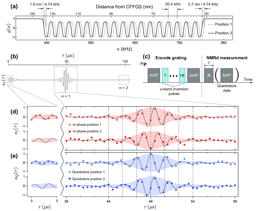
Figure 4: NMRd data measured for the $18\times$ diffraction grating. (a) Inversion profile for the two positions ($g_{1}$ and $g_{2}$) of the periodic grating encoded with a period of 20.4 kHz. The top horizontal axis indicates the position-dependence of $g_{1}$ and $g_{2}$ with respect to the CFFGS. The shift in position corresponding to $\Delta u=4.74$ kHz is indicated for the regions of the sample that are 50 nm and 140 nm away from the CFFGS. (b) Calculated in-phase component $s_{I}(\tau)$ for the grating at position 1 given the simulated $g_{1}(u)$ profile in (a) and measured $p(u)$ shown in Fig. 3(b). (c) NMRd pulse sequence: the encoding part of the sequence encodes either $g_{1}(u)$ or $g_{2}(u)$ in (a) by applying 18 consecutive inversions. The second part of the sequence performs the NMRd readout. $s_{I}(\tau)$ is measured by applying a resonant RF pulse $(\mathbf{x})$ for a a duration $\tau$. An extra adiabatic half-passage pulse is applied for detecting the quadrature component $s_{Q}(\tau)$. (d, e) $s_{I}(\tau)$ and $s_{Q}(\tau)$ measurements for the two grating positions in (a) as a function of the effective encoding time $\tau$. The shaded regions in (d, e) indicate the signal amplitude.

We detect the statistical spin fluctuations in an ensemble of approximately $2\times 10^{6}$ ³¹P spins within the conical region of the InP sample indicated in Fig. 3(a) (see Sec. III of Ref. [21]), using the MAGGIC spin detection protocol described in Ref. [16]. The measured signal is proportional to the integrated $z$-axis magnetization $s\propto\int\,du\,p(u)\expectationvalue{\sigma_{z}}_{u}$ (see Appendix A), where $\expectationvalue{\sigma_{z}}_{u}$ is the expectation value of the Pauli $z$ operator for a spin at Rabi frequency $u$ determined by the NMR encoding sequence used in the MAGGIC protocol, and $p(u)$ is the Rabi-frequency distribution (see Appendix A), determined both by the geometry of the sample as well as the detection protocol which constrains the effective measurement volume near the CFFGS. We experimentally determine $p(u)$ [Fig. 3(b)] using the Fourier encoding method presented in [16].

We encode the periodic grating $g(u)=\expectationvalue{\sigma_{z}}_{u}$ by selectively inverting sequential regions in the sample that are 10.2-kHz wide and separated by 10.2 kHz in $u$, as indicated by Fig. 4(a). The physical regions targeted by the inversions are shown in Fig. 3(a). To generate a particular $g(u)$, we implement control waveforms that invert spins within the range $(u_{\text{low}},u_{\text{high}})$ with adjustable edge sharpness around $u_{\text{low}}$ and $u_{\text{high}}$. To verify the performance of the inversion waveform, we implement a control sequence, shown in Fig. 3(c), that targets spins within a 100-kHz bandwidth: $562.5\,\text{kHz}\leq u\leq 662.5\,\text{kHz}$. The measured Rabi-frequency distribution after the application of the band-inversion pulse [Fig. 3(d)] agrees closely with the expected inversion profile. Further details regarding the band-inversion pulses are in Sec. IV(B) of Ref. [21], which also includes an animation depicting the operation of the 100 kHz-wide band-inversion pulse.

The NMRd protocol used to measure $g(u)$ is shown schematically in Fig. 4(c). After encoding the grating, we apply a Larmor-frequency RF pulse for a duration $\tau$. The evolution of the spin starting from the state $\rho_{0}\propto\sigma_{z}$, when driven with constant Rabi frequency $u$ is described by a unitary $U(u,\tau)=\exp(-i2\pi u\tau\sigma_{x}/2)$ in the frame rotating at $\omega_{0}$. The in-phase $(s_{I})$ and quadrature $(s_{Q})$ components of diffraction signal are the ensemble-averaged expectation values of $\sigma_{z}$ and $\sigma_{y}$:

$$\begin{bmatrix}s_{I}(\tau)\\ s_{Q}(\tau)\end{bmatrix} =\int_{0}^{\infty}\,du\,p(u)\,g(u)\begin{bmatrix}\mathrm{Tr}\big{[}\sigma_{z}U(u,\tau)\rho_{0}U^{\dagger}(u,\tau)\big{]}\\[5.0pt] \mathrm{Tr}\big{[}\sigma_{y}U(u,\tau)\rho_{0}U^{\dagger}(u,\tau)\big{]}\end{bmatrix}$$

$$\propto\int_{0}^{\infty}\,du\,p(u)\,g(u)\begin{bmatrix}\cos(2\pi u\tau)\\ \sin(2\pi u\tau)\end{bmatrix}.$$ (1)

To measure the quadrature part of NMRd signal, we end the measurement sequence with a numerically-optimized adiabatic half-passage (AHP) pulse that rotates $\sigma_{y}$ to $\sigma_{z}$. It can be seen that if $g(u)$ has a single modulation period $\Omega$, i.e., $g(u+n\Omega)=g(u)$, $n\in\mathbb{Z}$, and varies much more rapidly than the envelope of $p(u)$, then $s_{I}(\tau)$ and $s_{Q}(\tau)$ contain a series of diffraction echos separated by $1/\Omega$-long intervals. The amplitudes of these echos reflect the magnitude of the Fourier coefficients of $g(u)$, and the echo envelopes contain the Fourier transform of $p(u)$.

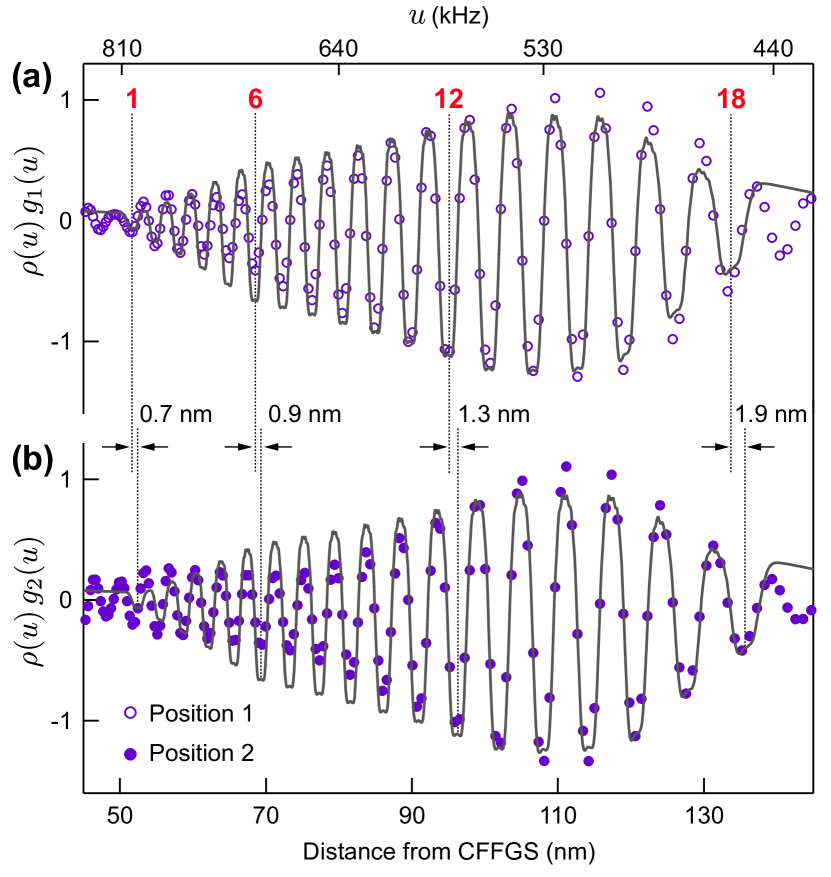
Figure 5: Coordinate-space reconstruction of the diffraction grating. Solid lines in (a) and (b) are the calculated $p(u)g_{1}(u)$ $[p(u)g_{2}(u)]$ using $g_{1}(u)$ $[g_{2}(u)]$ in Fig. 4(a) and $p(u)$ in Fig. 3(b). The solid dots are the coordinate-space reconstructions of $p(u)g_{1}(u)$ and $p(u)g_{2}(u)$ by Fourier transforming the data in Fig. 4 after padding it with zeroes. The position values indicated on the lower horizontal axis are determined from the simulated field distribution produced by the CFFGS (see Sec. II of Ref. [21]).The dashed vertical lines are placed as a guide to indicate the spatial offset between the two grating positions. The number of the inversion slice is indicated above the vertical lines.

To demonstrate the phase sensitivity of NMRd, we encode two spin magnetization gratings $g_{1}(u)$ and $g_{2}(u)$, shown in Fig. 4(a), that differ by a 4.74 kHz translation, i.e., $g_{2}(u)=g_{1}(u+4.74~{}\text{kHz})$. We refer to $g_{1}(u)$ and $g_{2}(u)$ as the grating at position 1 and 2, respectively. The physical displacement of the grating corresponding to $\Delta u=4.74~{}\text{kHz}$ is $\Delta z=0.7$ nm ($\Delta z=1.9$ nm) at $z=50$ nm ($z=140$ nm). Both gratings are produced using the control sequences shown in Fig. 4(c) that comprise 18 band inversion waveforms sandwiched between two AHPs identical to the ones used to measure $s_{Q}(\tau)$.

Fig. 4(b) shows a plot of the expected $s_{I}(\tau)$ calculated using Eq. (1), $g_{1}(u)$, and the measured $p(u)$ shown in Fig. 3(b). Because the first DE at $\tau\sim 49~{}\mu\text{s}$ has a significantly larger amplitude than the higher diffraction orders, we measure the NMRd signal only for $n=1$, for both grating positions, in the interval $39~{}\mu\text{s}\leq\tau\leq 59~{}\mu\text{s}$, using the NMRd measurement protocol is shown in Fig. 4(c). We note that for all measurements shown in Fig. 4, the maximum duration of the resonant RF pulse used in the NMRd measurement portion of the sequence was $59\,\mu\text{s}$, which is much shorter than the transverse relaxation time $T_{2\rho}=570\,\mu\text{s}$ measured under a continuous resonant RF drive (see Sec. V of Ref. [21]). Therefore, we ignore decoherence effects during the Rabi pulse in our analysis and simulations. The resulting data are shown in Fig. 4(d, e), which also include the un-scaled calculated values for $s_{I}(\tau)$ and $s_{Q}(\tau)$. The echo envelopes for both signal quadratures are shown as the shaded regions in Fig. 4(d, e). We see that although the small shift in the grating position produces little discernible change in the echo envelope, it is clearly visible in the change in the relative phase of the in-phase and quadrature measurements, demonstrating the importance of phase-sensitive detection for high-precision position measurements.

In Sec. VI(A, B) of Ref. [21], we construct a statistical estimator [25] to determine the periodicity $\Omega$ from the measured data. The calculation is done assuming no prior knowledge of $g(u)$, other than the fact that it is periodic in $u$, and varies more rapidly than $p(u)$. The resulting estimates for $\Omega$ in $g_{1}$ and $g_{2}$ are $\Omega_{1}=20.30\pm 0.14$ kHz and $\Omega_{2}=20.26\pm 0.10$ kHz, respectively. The 0.14 kHz (0.10 kHz) error in the period of $g_{1}$ ($g_{2}$) in $u$-space corresponds to an uncertainty of 0.2 Å (0.15 Å) in the wavelength of the grating at $z=50$ nm and 0.6 Å (0.4 Å) at $z=140$ nm.

In Sec. VI(C, D) of Ref. [21], we construct a maximum likelihood estimator for $\Delta u$ for the data in Fig.4, which yields $\Delta u=4.67\pm 0.20$ kHz, in excellent agreement with the expected value of $\Delta u=4.74\,\text{kHz}$. The error in $\Delta u$ corresponds to an uncertainty of 0.3 Å (0.8 Å) in the relative $z-$axis position of $g_{1}$ ($g_{2}$) at $z=50$ nm ($z=140$ nm).

We reconstruct the periodic spin modulation in coordinate space by calculating the real part of the complex Fourier transform $\real\{\mathcal{F}^{-1}[s_{I}(\tau)+i\,s_{Q}(\tau)]\}$ using the data shown in Fig. 4(d, e) for the two grating positions. In the reconstruction, we include the points around the $n=1$ DE, as well as the points sampled near $\tau=0$ to account for a small DC offset in the modulation envelope caused by a slight asymmetry in the magnitude of the positive and negative amplitude regions in $g(u)$. The time records used in the Fourier transforms are constructed to be continuous by zero-padding the un-sampled regions in the interval $0\leq\tau\leq 59.5~{}\mu\text{s}$ [see Fig. 4(b)]. The data in the interval $0\leq\tau\leq 3\,\mu\text{s}$ is not expected to change for the two grating positions. Therefore, this interval was measured only for position 1 and used in the reconstruction of both grating positions. We see that the position-space representation of $p(u)g_{1}(u)$ and $p(u)g_{2}(u)$, shown in Fig. 5, closely follow the calculated values.

V Displacement Detection via NMR Interferometry

In Sec. IV, we performed phase-sensitive NMRd measurements of a nanometer-scale periodic modulation of the $z$-axis magnetization with sub-Ångstrom precision. In this section, we describe an interferometric detection protocol that enables us to measure a real-space displacement of the InP sample in the $z$ direction with a precision of 0.07 Å. The protocol, shown schematically in Fig. 6(a), utilizes the symmetric magic echo (SME) [20] NMR sequence to decouple the P-P and P-In interactions, thereby extending the coherence time of the ³¹P spins up to 12.8 ms. In Sec. IV(D) of Ref. [21], we describe a modification to the SME4 that allows us to evolve the spins under the Rabi field gradient for a variable amount of time $\Delta\tau$ for phase encoding. By extending the spin coherence time into the millisecond range and by utilizing the large Rabi field gradients of order $2\times 10^{5}$ T/m, we encode a helical phase winding in the $xz$ plane with an average wavelength as short as a few Ångstroms, allowing us to detect displacements of the InP sample with picometer precision.

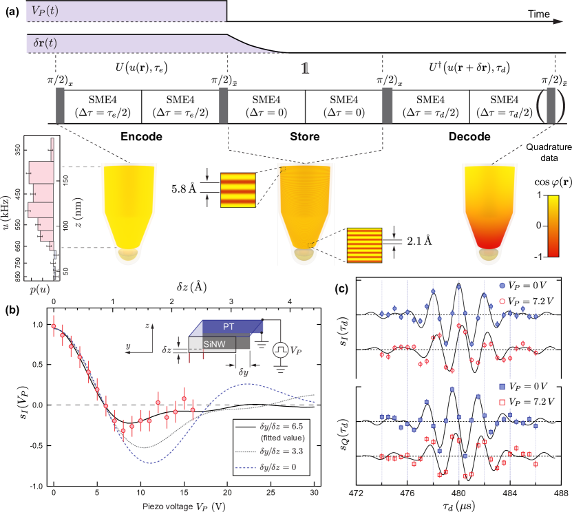
Figure 6: (a) Pulse sequence used for interferometric displacement detection, as well as the the voltage $V_{P}(t)$ applied to the PT, and the PT displacement $\delta\mathbf{r}(t)$. The unitary operations corresponding to different parts of the sequence are indicated above each block. The data presented in (b, c) were acquired from spins in the Rabi frequency range $400\,\text{kHz}<u<650$ kHz, corresponding to the sample volume indicated by the shaded regions in (a). The shading indicates the $z$-axis modulation $[\cos\varphi(\mathbf{r})]$ at different times during the measurement sequence, corresponding to $\tau_{e}=\tau_{d}=960\,\mu\text{s}$, and a sample displacement of $\delta z=1$ Å. (b) The data were acquired using the sequence shown in (a), where $2\times$SME4 sequences were used in the encoding portion, with each SME4 designed to generate a Rabi gradient evolution time of $\Delta\tau=480\,\mu\text{s}$. From the fit to the data, we determine the ratio $\delta y/\delta z=6.5$. For reference, two other curves have been included that show the variation in signal amplitude for different ratios of $\delta y/\delta z$. The calculations clearly indicate that for lateral displacements of order 1 nm, a higher ratio $\delta y/\delta z$ primarily increases the decay rate with respect to $V_{P}$ of the modulation envelope of the interference signal, without significantly affecting the modulation frequency; the modulation frequency, on the other hand, is primarily determined by $\delta z$. The asymmetry in the response along the $y$ and $z$ directions is caused by the relative magnitude of the Rabi field gradients near the center of the CFFGS, which is at least a factor of 100 larger in the $z$ direction than in the $y$ and $x$ directions. (c) In-phase and quadrature data were acquired for $V_{P}=0\,V$ and $V_{P}=7.2\,V$ with a fixed encoding time of $\tau_{e}=480\,\mu\text{s}$ for different decoding times. A single SME4 with $\Delta\tau=480\,\mu\text{s}$ was used for the encoding and decoding parts of the sequence. The displacement results in a shift in the phase of both signal quadratures. From the fit to the data, we determine displacement corresponding to $V_{P}=7.2\,V$ to be $\delta z=0.81\pm 0.07$ Å  and $\delta y=9.72\pm 1.34$ Å. The value of $\delta y$ determined from the fit is consistent with the value $\delta y=1.0\,\text{nm}$ determined by optical interferometry (see Sec. VII of Ref. [21].)

The protocol starts by encoding a helical winding for a time $\tau_{e}$. The density matrix for a spin at position $\mathbf{r}$ after encoding is $\rho_{1}=U\left[u(\mathbf{r}),\tau_{e}\right]\rho_{0}U^{\dagger}\left[u(\mathbf{r}),\tau_{e}\right]$, where $U\left[u(\mathbf{r}),\tau\right]=\exp\left[{-i2\pi\tau\sigma_{y}u(\mathbf{r})/2}\right]$. During this time, a constant voltage is applied to the PT [inset in Fig. 6(b)], which translates the InP sample with respect to the CFFGS, thereby slightly shifting the local field experienced by the ³¹P spins during encoding. The PT is retracted to its equilibrium position by zeroing the voltage. During retraction, $2\times$SME4 sequences with $\Delta\tau=0$ are applied, i.e., no gradient evolution, which refocus the homonuclear dipolar and $\sigma_{z}$ evolution during the time that the PT returns to its equilibrium position. The duration of the $2\times$SME4 sequences is 1.8 ms, which is chosen to be substantially longer than the $\sim 300\,\mu\text{s}$ mechanical response time of the PT. In the decoding phase, the inverse unitary $U^{\dagger}\left[u(\mathbf{r}+\delta\mathbf{r}),\tau_{d}\right]=\exp\left[i2\pi\tau_{d}u(\mathbf{r}+\delta\mathbf{r})\sigma_{y}/2\right]$ is applied for a time $\tau_{d}$ at the new location of the InP sample. The density matrix at the end of the sequence is $\rho_{2}=\delta U\rho_{0}\delta U^{\dagger}\propto\sigma_{z}\cos\varphi(\mathbf{r})+\sigma_{x}\sin\varphi(\mathbf{r})$, with $\delta U=\exp[-i\varphi(\mathbf{r})\sigma_{y}/2]$. The differential phase $\varphi(\mathbf{r})=2\pi\left[u(\mathbf{r})\tau_{e}-u(\mathbf{r}+\delta\mathbf{r})\tau_{d}\right]$ results from the interference of the encoding and decoding modulations separated by $\delta\mathbf{r}$. The measured signal quadratures at the end of the sequence are

$$\begin{bmatrix}s_{I}(\tau_{e},\tau_{d},\delta\mathbf{r})\\ s_{Q}(\tau_{e},\tau_{d},\delta\mathbf{r})\end{bmatrix}\propto\int d^{3}r\,\rho(\mathbf{r})\begin{bmatrix}\cos\varphi(\mathbf{r})\\ \sin\varphi(\mathbf{r})\end{bmatrix}$$ (2)

Here, $\rho(\mathbf{r})$ is the effective spin density at location $\mathbf{r}$ (see Appendix A).

Figure 6(b) shows a plot of the in-phase data acquired as a function of the voltage $V_{P}$ applied to the PT, using the sequence shown in Fig. 6(a), with $\tau_{d}=\tau_{e}=960~{}\mu\text{s}$. The modulation wavelength varies from $2.1$ Å  to $5.8$ Å  within the measured volume of the sample. To extract the $z$-displacement from the data, we conduct a least-squares fit [26] using Eq. (2), where we assume that $\delta\mathbf{r}\propto V_{P}$ and $\delta\mathbf{r}=\delta y~{}\hat{\mathbf{y}}+\delta z~{}\hat{\mathbf{z}}$, with the fit parameters being the PT coefficient $\delta z/V_{P}$ and $\delta y/\delta z$. The displacement in the $y$ direction is included because the PT used for the measurements was poled in the $y$ direction; hence $\delta y(V_{P})\gg\delta z(V_{P})$. The effective spin density $\rho(\mathbf{r})$ was calculated using our model for the sample geometry (Sec. III of Ref. [21]). For details regarding the characterization of the PT, see Sec. VII of Ref. [21]. The resulting fit is indicated by the solid line in Fig. 6(b), corresponding to a displacement $\delta z/V_{P}=0.15\pm 0.01$ Å/V. The PT calibration was used to derive the top horizontal axis of Fig. 6(b).

Finally, we conduct a set of measurements in which we keep the encoding time and the voltage step applied to the PT constant, and vary the decoding time. Fig. 6(c) shows the in-phase and quadrature data acquired for $V_{P}=0$ V and $V_{P}=7.2$ V with $\tau_{e}=480\,\mu\text{s}$. To extract the sample displacement, we fit to the data using Eq. (2), with the fit parameters being $\delta z$ and $\delta y$ [solid lines in Fig. 6(c)]. The fit yields a sample displacement of $\delta z=0.81\pm 0.07$ Å. In Sec. VIII of Ref. [21], we also provide an alternative fitting method, which utilizes the measured $p(u)$ distribution instead of the geometric model of the sample. Consistent with the previous method, the fit yields $\delta z=0.85\pm 0.07$ Å.

Using the PT displacement calibration found from Fig. 6(b), we would expect the displacement corresponding to $V_{P}=7.2$ V to be $\delta z=1.04\pm 0.04$ Å. Although the calculated displacements from the two measurements are in reasonable agreement, the 20% difference in $\delta z$ could be caused by systematic errors in the different methods used for determining the displacement corresponding to $V_{P}=7.2$ V. In particular, to determine the PT displacement for the data in Fig. 6(b), we needed to assume a particular functional form for the piezo characteristic $\delta\mathbf{r}(V_{P})$. For the data in Fig. 6(c), however, we find the displacement directly for one particular value of $V_{P}$, without any assumptions on $\delta\mathbf{r}(V_{P})$. It is therefore possible that a small nonlinear component in $\delta\mathbf{r}(V_{P})$ could be responsible for the observed difference.

For measurements that require large encoding wavevectors, such as those that would be needed for crystallographic NMRd, the mechanical stability of the sample becomes an important consideration. To characterize the response to mechanical motion, we calculate the root-mean-square integrated phase error $\delta\varphi(\omega)$, caused by the motion of the sample relative to the gradient source during the encoding sequence. As an example, Fig. 7 shows a plot of $\delta\varphi(\omega)$ calculated for the sequence shown in Fig. 6(a). We can clearly see that at low frequencies, even Ångstrom-scale motion can introduce large phase errors. In particular, the main peak near 100 Hz is caused by a 1 Å-peak motion near the frequency $1/(2T)$, where $T$ is the duration of the entire sequence; the smaller peak near 5 kHz represents the motion at $1/\tau_{\text{ME}}$, where $\tau_{\text{ME}}$ is the duration of a single magic echo sequence. Overall, however the phase error decreases substantially for frequencies $\omega/(2\pi)>100\,\text{kHz}$, near the SiNW mechanical resonance, where the Ångstrom-scale motion of the oscillator caused by thermal fluctuations would be of concern. Phase errors can be further minimized by applying feedback cooling to reduce the motion of the oscillator [23]. For the measurements reported here, the encoding direction is perpendicular to the oscillation direction of the SiNW, which greatly reduces phase errors caused by the resonant motion of the oscillator. To ensure that such errors are negligible, we compare the measured the signal after applying the sequence in Fig. 6(a) at zero piezo voltage, with $\tau_{e}=\tau_{d}=0$ and $\tau_{e}=\tau_{d}=960\ \mu$s – the longest encoding time used in this work. The result shows a small $11\pm 10\%$ reduction at $960\ \mu$s encoding, which indicates sufficient mechanical stability in the reported experiments.

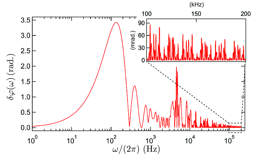
Figure 7: Phase error $\delta\varphi(\omega)$ calculated by integrating the phase accumulated by a ³¹P spin oscillating at frequency $\omega$ with a peak amplitude of 1 Å  in the $z$ direction and experiencing the sample-averaged Rabi-field gradient of ${\partial B_{1}/\partial z}=1.8$ G/nm. For the calculation, we use the sequence in Fig. 6(a) with $\tau_{\text{ME}}=212\,\mu\text{s}$ and $T=5.1$ ms.

VI Conclusions

In this work, we presented two experiments that utilize the large encoding wavevectors generated in a nanoMRI setting to realize phase-sensitive position measurement of ³¹P spins with sub-Ångstrom precision. These results demonstrate new capabilities for studying material structure and quantum phenomena by extending the the spectroscopic and imaging capabilities of NMR to the atomic scale. Although the concept of NMRd was first envisioned for the study of material structure, it can be applied more generally to study the dynamics of spatially-periodic spin correlations. For example, experiment presented in Sec. V can be readily adapted to study quantum transport by replacing the storage period with an evolution under an effective Hamiltonian. In fact, such experiments have been performed to study dipolar spin diffusion of ¹⁹F spins in $\text{CaF}_{2}$ on the micron scale [27]. Here, we have demonstrated the ability to generate encoding wavevectors that are nearly a factor of $10^{4}$ times larger than these previous works, which could be used to probe spin transport on length scales as short as the lattice spacing, where quantum phenomena could become important. In addition, the interferometric method introduced in this work to measure displacement could be extended to study molecular motion on the Ångstrom scale using Fourier imaging techniques. More generally, atomic-scale NMRd could be applied to Hamiltonian engineering applications by providing local control of spins in periodic spin systems [28], and for probing correlations in nuclear spin chains, where novel quantum many-body correlations have been observed [29].

The application of NMRd to study three-dimensional crystal structure will require devices capable of generating highly uniform field gradients. Upcoming experiments focusing on NMRd crystallography will utilize a new design that combines the CFFGS with four additional current carrying paths designed to generate highly uniform three-dimensional field gradients of order $3\times 10^{4}$ T/m with a maximum variation of 0.5% in a $\sim(100~{}\text{nm})^{3}$ volume, suitable for crystallographic NMRd measurements. Using these gradients, ¹H spins separated by 3 Å, for example, would form a DE at an encoding time of 2.6 ms, which is readily achievable using dynamical-decoupling NMR sequences, such as the SME. This capability could be used to study the structure of organic nanocrystalline materials, such as protein nanocrystals, that are of great interest in structural biology.

VII Acknowledgements

This work was undertaken thanks in part to funding from the U.S. Army Research Office through Grant No. W911NF1610199, the Canada First Research Excellence Fund (CFREF), and the Natural Sciences and Engineering Research Council of Canada (NSERC). The University of Waterloo’s QNFCF facility was used for this work. This infrastructure would not be possible without the significant contributions of CFREF-TQT, CFI, Industry Canada, the Ontario Ministry of Research and Innovation and Mike and Ophelia Lazaridis. Their support is gratefully acknowledged. H.H. would like to thank F. Flicker, S. H. Simon and H. S. Røising for insightful and inspiring discussions. R.B thanks D. G. Cory and A. Cooper for useful discussions.

H. Haas and S. Tabatabaei contributed equally to this work.

Appendix A Spin Detection Protocol

Here, we briefly discuss our measurement protocol, while referring to [16] and the supplements therein for further details. We use the MAGGIC protocol [31], shown in Fig. 8, to detect the force generated by the $z$-axis magnetization from the spin ensemble. The protocol is comprised of successive applications of a measurement block, separated by an NMR encoding block containing the spin control operations of interest – e.g., the sequences in Fig. 4(c) and Fig. 6(a) for our two experiments. The duration of each measurement block $(\tau_{0}=1.0~{}\text{s})$ is chosen to be shorter than the correlation time of $\tau_{m}=2.9$ s of the statistical fluctuations for the ³¹P spins, measured using the MAGGIC protocol.

The MAGGIC waveform [Fig. 8(b)] applied in each measurement block consists of two periods, during which the gradient $\partial B_{z}/\partial y$ is modulated at the resonant frequency of the SiNW. To avoid spurious electrical couplings to the SiNW, we ensure that the modulation waveform has no Fourier component at $\omega_{c}$ by applying a periodic $\pi$ phase shift to the gradient modulation. An adiabatic full passage (AFP) pulse is applied synchronously with the phase shifts, which creates a force from the spins that is on resonance with the SiNW. The average force correlation between two consecutive measurement blocks is

$$s\propto\int d^{3}r~{}n(\mathbf{r})G_{R}^{2}(\mathbf{r})\chi\big{(}u(\mathbf{r})\big{)}\langle\sigma_{z}\rangle_{\mathbf{r}},$$ (3)

where $n(\mathbf{r})$ is the spin density, $G_{R}(\mathbf{r})=\partial B_{z}(\mathbf{r})/\partial y$ is the peak amplitude of the readout gradient, $\langle\sigma_{z}\rangle_{\mathbf{r}}$ is the expectation value of $\sigma_{z}$ at positon $\mathbf{r}$ at the end of the NMR encoding block, and $\chi(u)$ is a filter function quantifying the performance of the AFPs at Rabi frequency $u$ [16]. From Eq. (3), we identify the effective spin density as $\rho(\mathbf{r})=n(\mathbf{r})G_{R}^{2}(\mathbf{r})\chi\big{(}u(\mathbf{r})\big{)}$.

In the case where the NMR encoding block sequence is only selective in Rabi frequency [e.g., the sequence in Fig. 4(c)], $\langle\sigma_{z}\rangle_{\mathbf{r}}$ is the same for spins experiencing equal Rabi frequencies, which simplifies Eq. (3) to $s\propto\int du~{}p(u)\langle\sigma_{z}\rangle_{u}$, where $p(u)$ is the effective Rabi-frequency distribution. Given the approximate one-to-one relationship between $z$ and $u$ in our sample volume, $p(u)$ can be written as

$$p(u)\approx\frac{\partial z(u)}{\partial u}\int_{-\infty}^{\infty}dx\int_{-\infty}^{\infty}dy~{}\rho\big{(}x,y,z(u)\big{)}.$$ (4)

For the measurement blocks, we utilized the 2.3 Rabi-cycle AFP presented in Ref. [30]. For the experiment in Sec. IV, the AFP was 4.8 $\mu$s long, with a near-unity fidelity over $480\text{ kHz}\leq u\leq 960\text{ kHz}$, and for the experiment in Sec. V, the pulse was rescaled to be 5.7 $\mu$s to target the Rabi range $400\text{ kHz}\leq u\leq 800\text{ kHz}$. In the latter experiment, we also restrict the detection volume to $u\leq 650$ kHz by including an additional waveform in the beginning of the NMR encoding block. Acting as a low-pass filter, the waveform evolves spins aligned with the $z$-axis to the transverse plane for $u>650$ kHz, which then dephase due to transverse relaxation. Spins experiencing $u\leq 650$ kHz are not affected (see Ref. [21]).

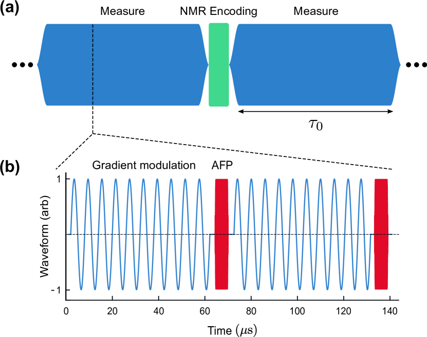
Figure 8: MAGGIC spin detection protocol. (a) General overview of the protocol. The blue regions indicate the spin readout period during which the MAGGIC waveform is applied. The correlation signal [Eq. (3)] is constructed from the average correlation of two consecutive force measurements made before and after the NMR encoding sequence. (b) The MAGGIC waveform primitive.

See pages 1,,,2,,3,,4,,5,,6,,7,,8,,9,,10,,11,,12,,13,,14,,15,,16,,17,,18,,19,,20 of supp.pdf

References

- Ajoy et al. [2015] A. Ajoy, U. Bissbort, M. D. Lukin, R. L. Walsworth, and P. Cappellaro, Atomic-Scale Nuclear Spin Imaging Using Quantum-Assisted Sensors in Diamond, Phys. Rev. X 5, 011001 (2015).
- Perunicic et al. [2016] V. S. Perunicic, C. D. Hill, L. T. Hall, and L. C. Hollenberg, A Quantum Spin-Probe Molecular Microscope, Nat. Commun. 7, 12667 (2016).
- Schirhagl et al. [2014] R. Schirhagl, K. Chang, M. Loretz, and C. L. Degen, Nitrogen-Vacancy Centers in Diamond: Nanoscale Sensors for Physics and Biology, Annu. Rev. Phys. Chem. 65, 83 (2014).
- Casola et al. [2018] F. Casola, T. V. D. Sar, and A. Yacoby, Probing Condensed Matter Physics with Magnetometry based on Nitrogen-Vacancy Centres in Diamond, Nat. Rev. Mater. 3, 17088 (2018).
- Rugar et al. [2004] D. Rugar, R. Budakian, H. J. Mamin, and B. W. Chui, Single Spin Detection by Magnetic Resonance Force Microscopy, Nature 430, 329 (2004).
- Grinolds et al. [2013] M. S. Grinolds, S. Hong, P. Maletinsky, L. Luan, M. D. Lukin, R. L. Walsworth, and A. Yacoby, Nanoscale Magnetic Imaging of a Single Electron Spin under Ambient Conditions, Nat. Phys. 9, 215 (2013).
- Willke et al. [2019] P. Willke, K. Yang, Y. Bae, A. J. Heinrich, and C. P. Lutz, Magnetic Resonance Imaging of Single Atoms on a Surface, Nat. Phys. 15, 1005 (2019).
- Lovchinsky et al. [2016] I. Lovchinsky, A. O. Sushkov, E. Urbach, N. P. de Leon, S. Choi, K. D. Greve, R. Evans, R. Gertner, E. Bersin, C. Müller, L. McGuinness, F. Jelezko, R. L. Walsworth, H. Park, and M. D. Lukin, Nuclear Magnetic Resonance Detection and Spectroscopy of Single Proteins using Quantum Logic, Science 351, 836 (2016).
- Degen et al. [2009] C. L. Degen, M. Poggio, H. J. Mamin, C. T. Rettner, and D. Rugar, Nanoscale Magnetic Resonance Imaging, Proc. Natl. Acad. Sci. U.S.A 106, 1313 (2009).
- Taminiau et al. [2012] T. H. Taminiau, J. J. Wagenaar, T. V. D. Sar, F. Jelezko, V. V. Dobrovitski, and R. Hanson, Detection and Control of Individual Nuclear Spins using a Weakly Coupled Electron Spin, Phys. Rev. Lett. 109, 137602 (2012).
- Zopes et al. [2018] J. Zopes, K. S. Cujia, K. Sasaki, J. M. Boss, K. M. Itoh, and C. L. Degen, Three-Dimensional Localization Spectroscopy of Individual Nuclear Spins with Sub-Angstrom Resolution, Nat. Commun. 9, 4678 (2018).
- Grob et al. [2019] U. Grob, M. D. Krass, M. Héritier, R. Pachlatko, J. Rhensius, J. Košata, B. A. Moores, H. Takahashi, A. Eichler, and C. L. Degen, Magnetic Resonance Force Microscopy with a One-Dimensional Resolution of 0.9 Nanometers, Nano Lett. 19, 7935 (2019).
- Rugar et al. [2015] D. Rugar, H. J. Mamin, M. H. Sherwood, M. Kim, C. T. Rettner, K. Ohno, and D. D. Awschalom, Proton Magnetic Resonance Imaging using a Nitrogen-Vacancy Spin Sensor, Nat. Nanotechnol. 10, 120 (2015).
- Arai et al. [2015] K. Arai, C. Belthangady, H. Zhang, N. Bar-Gill, S. J. DeVience, P. Cappellaro, A. Yacoby, and R. L. Walsworth, Fourier Magnetic Imaging with Nanoscale Resolution and Compressed Sensing Speed-up using Electronic Spins in Diamond, Nat. Nanotechnol. 10, 859 (2015).
- Ziem et al. [2019] F. Ziem, M. Garsi, H. Fedder, and J. Wrachtrup, Quantitative Nanoscale MRI with a Wide Field of View, Sci. Rep. 9, 12166 (2019).
- Rose et al. [2018] W. Rose, H. Haas, A. Q. Chen, N. Jeon, L. J. Lauhon, D. G. Cory, and R. Budakian, High-Resolution Nanoscale Solid-State Nuclear Magnetic Resonance Spectroscopy, Phys. Rev. X 8, 011030 (2018).
- Mansfield and Grannell [1973] P. Mansfield and P. K. Grannell, NMR ‘Diffraction’ in Solids?, J. Phys. C: Solid State Phys. 6, L422 (1973).
- Note [1] In MRI, is the encoding wavenumber corresponding to the spatial modulation of the nuclear spin magnetization, generated by the evolution of spins with gyromagnetic ratio in the magnetic field gradient for a time .
- Vachha and Huang [2021] B. Vachha and S. Y. Huang, MRI with Ultrahigh Field Strength and High-Performance Gradients: Challenges and Opportunities for Clinical Neuroimaging at 7 T and Beyond, Eur. Radiol. Exp 5, 35 (2021).
- Boutis et al. [2003] G. S. Boutis, P. Cappellaro, H. Cho, C. Ramanathan, and D. G. Cory, Pulse Error Compensating Symmetric Magic-Echo Trains, J. Magn. Reson. 161, 132 (2003).
- [21] See Supplemental Material for details of the sample attachment, CFFGS field distribution, sample geometry characterization, control sequences, supplementary measurements and further calculations, including videos of the sample attachment and the operation of the band inversion pulses.
- Sahafi et al. [2019] P. Sahafi, W. Rose, A. Jordan, B. Yager, M. Piscitelli, and R. Budakian, Ultralow Dissipation Patterned Silicon Nanowire Arrays for Scanning Probe Microscopy, Nano Lett. 20, 218 (2019).
- Poggio et al. [2007] M. Poggio, C. L. Degen, H. J. Mamin, and D. Rugar, Feedback Cooling of a Cantilever’s Fundamental Mode below 5 mK, Phys. Rev. Lett 99, 017201 (2007).
- Dalacu et al. [2012] D. Dalacu, K. Mnaymneh, J. Lapointe, X. Wu, P. J. Poole, G. Bulgarini, V. Zwiller, and M. E. Reimer, Ultraclean Emission from InAsP Quantum Dots in Defect-Free Wurtzite InP Nanowires, Nano Lett. 12, 5919 (2012).
- Casella and Berger [1990] G. Casella and R. Berger, Statistical Inference, Duxbury advanced series (Brooks/Cole Publishing Company, 1990).
- Sivia and Skilling [2006] D. Sivia and J. Skilling, Data Analysis: A Bayesian Tutorial, Oxford science publications (OUP Oxford, 2006).
- Zhang and Cory [1998] W. Zhang and D. G. Cory, First Direct Measurement of the Spin Diffusion Rate in a Homogenous Solid, Phys. Rev. Lett. 80, 1324 (1998).
- Ajoy and Cappellaro [2013] A. Ajoy and P. Cappellaro, Quantum Simulation via Filtered Hamiltonian Engineering: Application to Perfect Quantum Transport in Spin Networks, Phys. Rev. Lett. 110, 220503 (2013).
- Wei et al. [2018] K. X. Wei, C. Ramanathan, and P. Cappellaro, Exploring Localization in Nuclear Spin Chains, Phys. Rev. Lett. 120, 070501 (2018).
- Tabatabaei et al. [2021] S. Tabatabaei, H. Haas, W. Rose, B. Yager, M. Piscitelli, P. Sahafi, A. Jordan, P. J. Poole, D. Dalacu, and R. Budakian, Numerical Engineering of Robust Adiabatic Operations, Phys. Rev. Applied 15, 044043 (2021).
- Nichol et al. [2012] J. M. Nichol, E. R. Hemesath, L. J. Lauhon, and R. Budakian, Nanomechanical Detection of Nuclear Magnetic Resonance using a Silicon Nanowire Oscillator, Phys. Rev. B 85, 054414 (2012).