Sampling

Optimizing Pilot Spacing in MU-MIMO Systems Operating Over Aging Channels

Abstract

In the uplink of multiuser multiple input multiple output (MU-MIMO) systems operating over aging channels, pilot spacing is crucial for acquiring channel state information and achieving high signal-to-interference-plus-noise ratio (SINR). Somewhat surprisingly, very few works examine the impact of pilot spacing on the correlation structure of subsequent channel estimates and the resulting quality of channel state information considering channel aging. In this paper, we consider a fast-fading environment characterized by its exponentially decaying autocorrelation function, and model pilot spacing as a sampling problem to capture the inherent trade-off between the quality of channel state information and the number of symbols available for information carrying data symbols. We first establish a quasi-closed form for the achievable asymptotic deterministic equivalent SINR when the channel estimation algorithm utilizes multiple pilot signals. Next, we establish upper bounds on the achievable SINR and spectral efficiency, as a function of pilot spacing, which helps to find the optimum pilot spacing within a limited search space. Our key insight is that to maximize the achievable SINR and the spectral efficiency of MU-MIMO systems, proper pilot spacing must be applied to control the impact of the aging channel and to tune the trade-off between pilot and data symbols.

I Introduction

In wireless communications, pilot symbol-assisted channel estimation and prediction are used to achieve reliable coherent reception, and thereby to provide a variety of high quality services in a spectrum efficient manner. In most practical systems, the transmitter and receiver nodes acquire and predict channel state information by employing predefined pilot sequences during the training phase, after which information symbols can be appropriately modulated and precoded at the transmitter and estimated at the receiver. Since the elapsed time between pilot transmissions and the transmit power level of pilot symbols have a large impact on the quality of channel estimation, a large number of papers investigated the optimal spacing and power control of pilot signals in both single and multiple antenna systems [1, 2, 3, 4, 5, 6, 7, 8, 9, 10, 11, 12].

Specifically in the uplink of multiuser multiple input multiple output (MU-MIMO) systems, several papers proposed pilot-based channel estimation and receiver algorithms assuming that the complex vector channel undergoes block fading, meaning that the channel is constant between two subsequent channel estimation instances [13, 14, 15, 16]. In the block fading model, the evolution of the channel is memoryless in the sense that each channel realization is drawn independently of previous channel instances from some characteristic distribution. While the block fading model is useful for obtaining analytical expressions for the achievable signal-to-interference-plus-noise ratio (SINR) and capacity [15, 17], it fails to capture the correlation between subsequent channel realizations and the aging of the channel between estimation instances [6, 7, 11, 12].

Due to the importance of capturing the evolution of the wireless channel in time, several papers developed time-varying channel models, as an alternative to block fading models, whose states are advantageously estimated and predicted by means of suitably spaced pilot signals. In particular, a large number of related works assume that the wireless channel can be represented as an autoregressive (AR) process whose states are estimated and predicted using Kalman filters, which exploit the correlation between subsequent channel realizations [3, 4, 6, 10, 12]. These papers assume that the coefficients of the related AR process are known, and the current and future states of the process (and thereby of the wireless channel) can be well estimated. Other important related works concentrate on estimating the coefficients of AR processes based on suitable pilot-based observations and measurements [18, 19, 20]. In our recent work [12], it was shown that when an AR process is a good model of the wireless channel and the AR coefficients are well estimated, not only the channel estimation can exploit the memoryful property of the channel, but also a new MU-MIMO receiver can be designed, which minimizes the mean squared error (MSE) of the received data symbols by exploiting the correlation between subsequent channel states. It is important to realize that the above references build on discrete time AR models, in which the state transition matrix is an input of the model and can be estimated by some suitable system identification technique, such as the one proposed in [20]. However, these papers do not ask the question of how often the channel state of a continuous time channel should be observed by suitably spaced pilot signals to realize a certain state transition matrix in the AR model of the channel.

Specifically, a key characteristic of a continuous time Rayleigh fading environment is that the autocorrelation function of the associated stochastic process is a zeroth-order Bessel function, which must be properly modelled [21, 22]. This requirement is problematic when developing discrete-time AR models, since it is well-known that Rayleigh fading cannot be perfectly modelled with any finite order AR process (since the autocorrelation function of discrete time AR processes does not follow a Bessel function), although the statistics of AR process can approximate those of Rayleigh fading [23, 24].

Recognizing the importance of modeling fast fading, including Rayleigh fading, channels with proper autocorrelation function as a basis for pilot spacing optimization, papers [25, 26] use a continuous time process as a representation of the wireless channel, and address the problem of pilot spacing as a sampling problem. According to this approach, pilot placement can be considered as a sampling problem of the fading variations, and the quality of the channel estimate is determined by the density and accuracy of channel sampling [26]. However, these papers consider single input single output (SISO) systems, do not deal with the problem of pilot and data power control, and are not applicable to MU-MIMO systems employing a minimum mean squared error (MMSE) receiver, which was proposed in, for example, [12]. On the other hand, paper [6] analyzes the impact of channel aging on the performance of MIMO systems, without investigating the interplay between pilot spacing and the resulting state transition matrix of the AR model of the fast fading channel. The most important related works, their assumptions and key performance metrics are listed and compared with those of the current paper in Table I.

Table I: Overview of Related Literature

Reference	Block fading vs. Aging channel	Is AR modeling used?	Channel est.	SISO or MIMO receiver	Key performance indicators	Comment
Truong et al., [6]	channel aging between pilots	discrete time AR approximating a Bessel func.	MMSE based on known AR params	max. ratio combiner (MRC) receiver (not AR-aware)	average SINR, achievable rate	both UL and DL are considered
Zhang et al., [2]	channel aging between pilots	discrete time AR approximating a Bessel f.	adaptive est. of AR params	SISO joint channel and data est.	BER	AR(2) parameter estimation and demodulation
Savazzi and Spagnolini [25]	channel aging between pilots	AR channel evolution over estimation instances	interpolation based on multiple observations	SISO	average SINR and BER	power control is out of scope
Mallik et al., [16]	block fading channel	not applicable	MMSE channel estimation	SIMO with MRC	average SINR, symbol error probability	pilot/data power control is out of scope
Akin and Gursoy [27]	channel aging between pilots	discrete time first order AR (Gauss-Markov) process	MMSE channel estimation	SISO	achievable rate and bit energy $E_{b}/N_{0}$	optimal power distribution and training period for SISO are derived
Chiu and Wu [8]	channel aging between plots	discrete time AR model approximating a Rayleigh fading	Kalman filter assisted channel estimation	receiver structure is out-of-scope	MSE of channel est., data rate, capacity	pilot/data power control is out of scope
Fodor et al., [12]	no aging between pilots; correlated pilot intervals	discrete time AR(1) model	Kalman assisted ch. est.	AR(1)-aware MIMO MMSE receiver	MSE of the received data symbols	optimum pilot power control for AR(1) channels
Present paper	channel aging between pilots	AR(1) to model channel aging between pilots	MMSE interpolation by multiple observations	MU-MIMO with MMSE receiver	average (det. equivalent) SINR	both pilot spacing and pilot/data power control are considered

In this paper, we are interested in determining the average SINR in the uplink of MU-MIMO systems operating in fast fading as a function of pilot spacing, pilot/data power allocation, number of antennas and spatially multiplexed users. Specifically, we ask the following two important questions, which are not answered by previous works:

• What is the average SINR in a closed or quasi-closed form in the uplink of MU-MIMO systems in fast fading in the presence of antenna correlation? How does the average SINR depend on pilot spacing and pilot/data power control?

• What is the optimum pilot spacing and pilot/data power allocation as a function of the number of antennas and the Doppler frequency associated with the continuous time fast fading channel?

In the light of the above discussion and questions, the main contributions of the present paper are as follows:

• Proposition 1 derives the asymptotic deterministic equivalent SINR of any user in a MU-MIMO system in every data slot for fast fading channels that can be characterized by an associated AR process;

• Theorem 1 and Proposition 2 establish an upper bound on the achievable SINR as a function of pilot spacing, which is instrumental for determining the optimum pilot spacing.

• Proposition 3, building on Proposition 2, provides and upper bound on the average achievable spectral efficiency, which is instrumental in limiting the search space for the optimal frame size as a function of the Doppler frequency.

In addition, we believe that the engineering insights drawn from the numerical studies are useful when designing pilot spacing, for example in the form of determining the number of reference signals in an uplink frame structure, for MU-MIMO systems.

Specifically, to answer the above questions, we proceed as follows. In the next section, we present our system model, which admits correlated wireless channels between any of the single-antenna mobile terminal and the receive antennas of the base station (BS). Next, Section III focuses on channel estimation, which is based on subsequent pilot-based measurements and an MMSE-interpolation for the channel states in between estimation instances. Section IV proposes an algorithm to determine the average SINR. Section V studies the impact of pilot spacing and power control on the achievable SINR and the spectral efficiency (SE) of all users in the system. That section investigates the impact of pilot spacing on the achievable SINR and establishes an upper bound on this SINR. We show that this upper bound is monotonically decreasing as the function of pilot spacing. This property is very useful, because it enables to limit the search space of the possible pilot spacings when looking for the optimum pilot spacing in Section VI. That section also considers the special case when the channel coefficients associated with the different receive antennas are uncorrelated and identically distributed. It turns out that in this special case a simplified SINR expression can be derived. Section VII presents numerical results and discusses engineering insights. Finally, Section VIII draws conclusions.

II System Model

Figure 1: Pilot (P) and data (D) symbols in the time-frequency domains of the system in the $(0,(\Delta+1)T)$ interval. The solid line above the time-frequency resource grid represents the continuous time complex channel $\mathbf{h}(t)$, while the dashed line represents the MMSE channel estimate $\hat{\mathbf{h}}(t)$. Notice that in each time slot of length $T$ all symbols are either pilot or data symbols.

Table II: System Parameters

Notation	Meaning
$K$	Number of MU-MIMO users
$N_{r}$	Number of antennas at the BS
$F$	Number of frequency channels used for pilot and data transmission within one slot
$\Delta$	number of data slots in a data-pilot cycle
$\tau_{p}=F,\tau_{d}=\Delta F$	Number of pilot/data symbols within a coherent set of subcarriers
$\mathbf{s}\in\mathds{C}^{\tau_{p}\times 1}$	Sequence of pilot symbols
$x$	Data symbol
$P_{p},P$	Pilot power per symbol, data power per symbol
$\mathbf{Y}^{p}(t)\in\mathds{C}^{N_{r}\times\tau_{p}},y(t)\in\mathds{C}^{N_{r}}$	Received pilot and data signal at time $t$, respectively
$\alpha$	Large scale fading between the mobile station and the base station
$\mathbf{C}\in\mathds{C}^{N_{r}\times N_{r}}$	Stationary covariance matrix of the fast fading channel
$\mathbf{h}(t),\hat{\mathbf{h}}(t)\in\mathds{C}^{N_{r}}$	Fast fading channel and estimated channel
$\bm{\varepsilon}(t)\in\mathds{C}^{N_{r}},\bm{\Sigma}\in\mathds{C}^{N_{r}\times N_{r}}$	Channel estimation error and its covariance matrix
$\mathbf{G}^{\star}$	Optimal MU-MIMO receiver.
$f_{D}$	Maximum Doppler frequency
$T$	Slot duration

II-A Uplink Pilot Signal Model

By extending the single antenna channel model of [25], each transmitting mobile station (MS) uses a single time slot to send $F$ pilot symbols, followed by $\Delta$ time slots, each of which containing $F$ data symbols according to Figure 1. Each symbol is transmitted within a coherent time slot of duration $T$. Thus, the total frame duration is $(1+\Delta)T$, such that each frame consists of 1 pilot and $\Delta$ data time slots, which we will index with $i=1\ldots\Delta$. User-$k$ transmits each of the $F$ pilot symbols with transmit power $P_{p,k}$, and each data symbol in slot-$i$ with transmit power $P_{k}(i),\leavevmode\nobreak\ k=1\ldots K$. To simplify notation, in the sequel we tag User-1, and will drop index $k=1$ when referring to the tagged user.

Assuming that the coherence bandwidth accommodates at least $F$ pilot symbols, this system allows to create $F$ orthogonal pilot sequences. To facilitate spatial multiplexing and channel state information at the receiver (CSIR) acquisition at the BS, the MSs use orthogonal complex sequences, such as shifted Zadoff-Chu sequences of length $\tau_{p}=F$, which we denote as:

$$\mathbf{s} \triangleq\left[s_{1},...,s_{\tau_{p}}\right]^{T}\in\mathds{C}^{{\tau_{p}\times 1}},$$ (1)

whose elements satisfy $|s_{i}|^{2}=1$. Under this assumption, the system can spatially multiplex $K\leq F$ MSs. Focusing on the received pilot signal from the tagged user at the BS, the received pilot signal takes the form of [12]:

$$\mathbf{Y}^{p}(t) =\alpha\sqrt{P_{p}}\mathbf{h}(t)\mathbf{s}^{T}+\mathbf{N}(t)\leavevmode\nobreak\ \leavevmode\nobreak\ \in\mathds{C}^{N_{r}\times\tau_{p}},$$ (2)

where $\mathbf{h}(t)\in\mathds{C}^{N_{r}\times 1}\sim\mathcal{CN}(\mathbf{0},\mathbf{C})$, that is, $\mathbf{h}(t)$ is a complex normal distributed column vector with mean vector $\mathbf{0}$ and covariance matrix $\mathbf{C}\in\mathds{C}^{N_{r}\times N_{r}}$. Furthermore, $\alpha$ denotes large scale fading, $P_{p}$ denotes the pilot power of the tagged user, and $\mathbf{N}(t)\in\mathds{C}^{N_{r}\times\tau_{p}}$ is the additive white Gaussian noise (AWGN) with element-wise variance $\sigma_{p}^{2}$. It will be convenient to introduce $\mathbf{\tilde{Y}}^{p}(t)$ by stacking the columns of $\mathbf{Y}^{p}(t)$ as:

$$\mathbf{\tilde{Y}}^{p}(t)=\textbf{vec}\big{(}\mathbf{Y}^{p}(t)\big{)}=\alpha\sqrt{P_{p}}\mathbf{S}\mathbf{h}(t)+\mathbf{\tilde{N}}(t)\leavevmode\nobreak\ \in\mathds{C}^{\tau_{p}N_{r}\times 1},$$ (3)

where vec is the column stacking vector operator, $\mathbf{\tilde{Y}}^{p}(t)$, $\mathbf{\tilde{N}}(t)\in\mathds{C}^{\tau_{p}N_{r}\times 1}$ and $\mathbf{S}\triangleq\mathbf{s}\otimes\mathbf{I}_{N_{r}}\in\mathds{C}^{\tau_{p}N_{r}\times N_{r}}$ is such that $\mathbf{S}^{H}\mathbf{S}=\tau_{p}\mathbf{I}_{N_{r}}$, where $\mathbf{I}_{N_{r}}$ is the identity matrix of size $N_{r}$.

II-B Channel Model

In (2), the channel $\mathbf{h}(t)$ evolves continuously according to a multivariate complex stochastic process with stationary covariance matrix $\mathbf{C}$. That is, for symbol duration $T$, the channel ($\mathbf{h}(t)$) evolves according to the following AR process:

$$\mathbf{h}(t+T) =\mathbf{A}\mathbf{h}(t)+\bm{\vartheta}(t),$$ (4)

where the transition matrix of the AR process is denoted by $\mathbf{A}$. This AR model has been commonly used to approximate Rayleigh fading channels in e.g. [28]. Equation (4) implies that the autocorrelation function of the channel process is:

$$\mathds{E}\left(\mathbf{h}(t)\mathbf{h}^{H}(t+iT)\right) =\mathbf{C}\left(\mathbf{A}^{H}\right)^{i},\quad\forall i.$$ (5)

Consequently, the autocorrelation function of the fast fading channel ($\mathbf{h}(t)$) is modelled as:

$$\mathbf{R}(i)\triangleq\mathds{E}\left(\mathbf{h}(t)\mathbf{h}^{H}(t+iT)\right) =\mathbf{C}e^{\mathbf{Q}^{H}iT},$$ (6)

where matrix $\mathbf{Q}$ describes the correlation decay, such that:

$$e^{\mathbf{Q}T}=\mathbf{A}.$$ (7)

Similarly, for user $k$,

$$\mathbf{R}_{k}(i)\triangleq\mathds{E}\left(\mathbf{h}_{k}(t)\mathbf{h}_{k}^{H}(t+iT)\right) =\mathbf{C}_{k}e^{\mathbf{Q}_{k}^{H}iT},$$ (8)

In each pilot slot, the BS utilizes MMSE channel estimation to obtain the channel estimate of each user, as it will be detailed in Section III. Without loss of generality, to simplify the notation, hereafter we assume that the time unit is $T$ and $iT=i$.

II-C Data Signal Model

When spatially multiplexing $K$ MU-MIMO users, the received data signal at the BS at time $t$ is [12]:

$$\mathbf{y}(t) =\underbrace{\mathbf{\alpha}\mathbf{h}(t)\sqrt{P}x(t)}_{\text{tagged user}}+\underbrace{\sum_{k=2}^{K}\mathbf{\alpha}_{k}\mathbf{h}_{k}(t)\sqrt{P_{k}}x_{k}(t)}_{\text{co-scheduled MU-MIMO users}}+\mathbf{n}_{d}(t),$$ (9)

where $\mathbf{y}(t)\in\mathds{C}^{N_{r}\times 1}$; and $x_{k}(t)$ denotes the transmitted data symbol of User-$k$ at time $t$ with transmit power $P_{k}$. Furthermore, $\mathbf{n}_{d}(t)\leavevmode\nobreak\ \sim\mathcal{CN}\left(\mathbf{0},\sigma_{d}^{2}\mathbf{I}_{N_{r}}\right)$ is the AWGN at the receiver.

III Channel Estimation

In this section, we are interested in calculating the MMSE estimation of the channel in each slot $i$, based on received pilot signals, as a function of the frame size corresponding to pilot spacing (see $\Delta$ in Figure 1). Note that estimating the channel at the receiver can be based on multiple received pilot signals both before and after the actual data slot $i$. While using pilot signals that are received before data slot $i$ requires to store the samples of the received pilot, using pilot signals that arrive after data slot $i$ necessarily induces some delay in estimating the transmitted data symbol. In the numerical section, we will refer to specific channel estimation strategies as, for example, "1 before, 1 after" or "2 before, 1 after" depending on the number of utilized pilot signals received prior to or following data slot $i$ for CSIR acquisition. In the sequel we use the specific case of "2 before, 1 after" to illustrate the operation of the MMSE channel estimation scheme, that is when the receiver uses the pilot signals $\mathbf{\tilde{Y}}^{p}(-\Delta-1)$, $\mathbf{\tilde{Y}}^{p}(0)$, and $\mathbf{\tilde{Y}}^{p}(\Delta+1)$ for CSIR acquisition. We are also interested in determining the distribution of the resulting channel estimation error, whose covariance matrix, denoted by $\mathbf{Z}(\Delta,i)$, will play an important role in subsequently determining the deterministic equivalent of the SINR.

III-A MMSE Channel Estimation and Channel Estimation Error

As illustrated in Figure 1, in each data slot $i$, the BS utilizes the MMSE estimates of the channel obtained in the neighboring pilot slots, for example at $(-\Delta-1)$, $0$ and $(\Delta+1)$, using the respective received pilot signals according to (3), that is $\mathbf{\tilde{Y}}^{p}\big{(}(-\Delta-1)\big{)}$, $\mathbf{\tilde{Y}}^{p}(0)$ and $\mathbf{\tilde{Y}}^{p}\big{(}(\Delta+1)\big{)}$, using the following lemma.

Lemma 1.

The MMSE channel estimator approximates the autoregressive fast fading channel in time slot $i$ based on the received pilots at $(-\Delta-1)$, $0$ and $(\Delta+1)$ as

$$\mathbf{\hat{h}}_{\textup{MMSE}}(\Delta,i)=\mathbf{H^{\star}}(\Delta,i)\mathbf{\hat{Y}}^{p}(\Delta),$$ (10)

where

$$\mathbf{H^{\star}}(\Delta,i)=\frac{1}{\alpha\sqrt{P_{p}}\tau_{p}}\mathbf{E}(\Delta,i).\big{(}\mathbf{M}(\Delta)+\mathbf{\Sigma}_{3}\big{)}^{-1}.(\mathbf{s}^{H}\otimes\mathbf{I}_{3N_{r}}),$$

$\mathbf{\hat{Y}}^{p}(\Delta)\triangleq\begin{bmatrix}\mathbf{\tilde{Y}}^{p}((-\Delta-1))\\ \mathbf{\tilde{Y}}^{p}(0)\\ \mathbf{\tilde{Y}}^{p}((\Delta+1))\end{bmatrix}$  and  $\mathbf{\Sigma}_{3}\triangleq\frac{\sigma_{p}^{2}}{\alpha^{2}P_{p}\tau_{p}}\mathbf{I}_{3N_{r}}$,

$$\mathbf{E}(\Delta,i) \triangleq\begin{bmatrix}\mathbf{R}(\Delta\!+\!1\!+\!i)&\mathbf{R}(i)&\mathbf{R}(\Delta\!+\!1\!-\!i)\end{bmatrix},$$ (11)

$$\mathbf{M}(\Delta) \triangleq\begin{bmatrix}\mathbf{C}&\mathbf{R}(\Delta\!+\!1)&\mathbf{R}(2\Delta\!+\!2)\\ \mathbf{R}^{H}(\Delta\!+\!1)&\mathbf{C}&\mathbf{R}(\Delta\!+\!1)\\ \mathbf{R}^{H}(2\Delta\!+\!2)&\mathbf{R}^{H}(\Delta\!+\!1)&\mathbf{C}\\ \end{bmatrix}.$$ (12)

Proof.

The MMSE channel estimator aims at minimizing the MSE between the channel estimate $\mathbf{\hat{h}}_{\textrm{MMSE}}(\Delta,i)=\mathbf{H}^{\star}(\Delta,i)\mathbf{\hat{Y}}^{p}(\Delta)$ and the channel $\mathbf{h}(i)$, that is

$$\mathbf{H^{\star}}(\Delta,i)=\text{arg}\min_{\mathbf{H}}\mathds{E}_{\mathbf{h},\mathbf{n}}\{||\mathbf{H}\mathbf{\hat{Y}}^{p}(\Delta)-\mathbf{h}(i)||^{2}\}.$$ (13)

The solution of this quadratic optimization problem is $\mathbf{H^{\star}}(\Delta,i)=\mathbf{a}(\Delta,i)^{H}\mathbf{F}^{-1}(\Delta)$ with

$$\mathbf{F}(\Delta) \triangleq\mathds{E}_{\mathbf{h},\mathbf{n}}\left(\mathbf{\hat{Y}}^{p}(\Delta)\left(\mathbf{\hat{Y}}^{p}(\Delta)\right)^{H}\right),$$ (14)

$$\mathbf{a}(\Delta,i) \triangleq\mathds{E}_{\mathbf{h},\mathbf{n}}\left(\mathbf{\hat{Y}}^{p}(\Delta)\mathbf{h}^{H}(i)\right).$$ (15)

Let

$$\mathbf{\bar{h}}(\Delta)\triangleq\begin{bmatrix}\mathbf{h}((-\Delta-1))\\ \mathbf{h}(0)\\ \mathbf{h}((\Delta+1))\end{bmatrix}$$

and

$$\mathbf{\tilde{\bar{N}}}(\Delta)\triangleq\begin{bmatrix}\mathbf{\tilde{N}}((-\Delta-1))\\ \mathbf{\tilde{N}}(0)\\ \mathbf{\tilde{N}}((\Delta+1))\end{bmatrix}.$$ (16)

Using $\mathbf{\bar{h}}(\Delta)$, we have

$$\begin{bmatrix}\mathbf{S}\mathbf{h}((-\Delta-1))\\ \mathbf{S}\mathbf{h}(0)\\ \mathbf{S}\mathbf{h}((\Delta+1))\end{bmatrix}=\begin{bmatrix}\mathbf{S}&\mathbf{0}&\mathbf{0}\\ \mathbf{0}&\mathbf{S}&\mathbf{0}\\ \mathbf{0}&\mathbf{0}&\mathbf{S}\end{bmatrix}\mathbf{\bar{h}}(\Delta)$$

$$\leavevmode\nobreak\ \leavevmode\nobreak\ \leavevmode\nobreak\ \leavevmode\nobreak\ \leavevmode\nobreak\ \leavevmode\nobreak\ \leavevmode\nobreak\ \leavevmode\nobreak\ =(\mathbf{I}_{3}\otimes\mathbf{S})\mathbf{\bar{h}}(\Delta)=(\mathbf{s}\otimes\mathbf{I}_{3N_{r}})\mathbf{\bar{h}}(\Delta).$$ (17)

Since $\mathbf{\bar{h}}(\Delta)$ and $\mathbf{\tilde{\bar{N}}}(\Delta)$ are independent and

$$\mathds{E}_{\mathbf{h},\mathbf{n}}(\mathbf{\bar{h}}(\Delta)\mathbf{\bar{h}}^{H}(\Delta)) =\mathbf{M}(\Delta),$$ (18)

$$\mathds{E}_{\mathbf{h},\mathbf{n}}(\mathbf{h}(i)\mathbf{\bar{h}}^{H}(\Delta)) =\mathbf{E}(\Delta,i).$$ (19)

Therefore, for $\mathbf{F}(\Delta)$ and $\mathbf{a}(\Delta,i)$, we have

$$\mathbf{F}(\Delta) =\mathds{E}_{\mathbf{h},\mathbf{n}}\left(\left(\alpha\sqrt{P_{p}}(\mathbf{I}_{3}\otimes\mathbf{S})\mathbf{\bar{h}}(\Delta)+\mathbf{\tilde{\bar{N}}}(\Delta)\right)\right.$$

$$\leavevmode\nobreak\ \leavevmode\nobreak\ \leavevmode\nobreak\ \leavevmode\nobreak\ \leavevmode\nobreak\ \leavevmode\nobreak\ \leavevmode\nobreak\ \leavevmode\nobreak\ \leavevmode\nobreak\ \leavevmode\nobreak\ \leavevmode\nobreak\ \leavevmode\nobreak\ \cdot\left.\left(\alpha\sqrt{P_{p}}(\mathbf{I}_{3}\otimes\mathbf{S})\mathbf{\bar{h}}(\Delta)+\mathbf{\tilde{\bar{N}}}(\Delta)\right)^{H}\right)$$

$$=\alpha^{2}P_{p}(\mathbf{I}_{3}\otimes\mathbf{S})\mathbf{M}(\Delta)\left(\mathbf{I}_{3}\otimes\mathbf{S}^{H}\right)+\sigma_{p}^{2}\mathbf{I}_{3N_{r}\tau_{p}},$$

$$\mathbf{a}(\Delta,i) =\mathds{E}_{\mathbf{h},\mathbf{n}}\left(\mathbf{\hat{Y}}(\Delta)\mathbf{h}^{H}(i)\right)$$

$$=\mathds{E}_{\mathbf{h},\mathbf{n}}\left(\left(\alpha\sqrt{P_{p}}(\mathbf{I}_{3}\otimes\mathbf{S})\mathbf{\bar{h}}(\Delta)+\mathbf{\tilde{\bar{N}}}(\Delta)\right)\mathbf{h}^{H}(i)\right)$$

$$=\alpha\sqrt{P_{p}}\leavevmode\nobreak\ (\mathbf{I}_{3}\otimes\mathbf{S})\leavevmode\nobreak\ \mathbf{E}(\Delta,i)^{T},$$

which yields Lemma 1. ∎

The MMSE estimate of the channel is then expressed as:

$$\mathbf{\hat{h}}_{\textrm{MMSE}}(\Delta,i)=\mathbf{H^{\star}}(\Delta,i)\mathbf{\hat{Y}}^{p}(\Delta)\leavevmode\nobreak\ \leavevmode\nobreak\ \leavevmode\nobreak\ \leavevmode\nobreak\$$

$$\leavevmode\nobreak\ \leavevmode\nobreak\ \leavevmode\nobreak\ \leavevmode\nobreak\ =\mathbf{H^{\star}}(\Delta,i)\left(\alpha\sqrt{P_{p}}(\mathbf{I}_{3}\otimes\mathbf{S})\mathbf{\bar{h}}(\Delta)+\mathbf{\tilde{\bar{N}}}(\Delta)\right)$$

$$\leavevmode\nobreak\ \leavevmode\nobreak\ \leavevmode\nobreak\ \leavevmode\nobreak\ =\frac{1}{\alpha\sqrt{P_{p}}\tau_{p}}\mathbf{E}(\Delta,i)\left(\mathbf{M}(\Delta)+\mathbf{\Sigma}_{3}\right)^{-1}$$

$$\leavevmode\nobreak\ \leavevmode\nobreak\ \leavevmode\nobreak\ \leavevmode\nobreak\ \leavevmode\nobreak\ \leavevmode\nobreak\ \leavevmode\nobreak\ \leavevmode\nobreak\ \leavevmode\nobreak\ \leavevmode\nobreak\ .\left(\alpha\sqrt{P_{p}}\tau_{p}\mathbf{\bar{h}}(\Delta)+\left(\mathbf{I}_{3}\otimes\mathbf{S}^{H}\right)\mathbf{\tilde{\bar{N}}}(\Delta)\right).$$ (20)

Next, we are interested in deriving the distribution of the estimated channel and the channel estimation error, since these will be important for understanding the impact of pilot spacing on the achievable SINR and spectral efficiency of the MU-MIMO system. To this end, the following two corollaries of Lemma 1 and (20) will be important in the sequel.

Corollary 1.

The estimated channel $\mathbf{\hat{h}}_{\textup{MMSE}}(\Delta,i)$ is a circular symmetric complex normal distributed vector $\mathbf{\hat{h}}_{\textup{MMSE}}(\Delta,i)\sim\mathcal{CN}\Big{(}\mathbf{0},\mathbf{\hat{\Phi}}_{\textup{MMSE}}(\Delta,i)\Big{)}$, with

$$\mathbf{\hat{\Phi}}_{\textup{MMSE}}(\Delta,i)\triangleq \mathds{E}_{\mathbf{h},\mathbf{n}}\{\mathbf{\hat{h}}_{\textup{MMSE}}(\Delta,i)\mathbf{\hat{h}}_{\textup{MMSE}}^{H}(\Delta,i)\}$$

$$= \mathbf{E}(\Delta,i)\big{(}\mathbf{M}(\Delta)+\mathbf{\Sigma}_{3}\big{)}^{-1}\mathbf{E}(\Delta,i)^{H}.$$ (21)

Proof.

Equation (1) follows directly from (20). ∎

An immediate consequence of Corollary 1 is the following corollary regarding the covariance of the channel estimation error, as a function of pilot spacing.

Corollary 2.

The channel estimation error in slot $i$, $\mathbf{\hat{h}}_{\textup{MMSE}}(\Delta,i)-\mathbf{h}(\Delta,i)$, is complex normal distributed with zero mean vector and covariance matrix given by:

$$\mathbf{Z}(\Delta,i)\triangleq\mathbf{C}-\mathbf{E}(\Delta,i)\big{(}\mathbf{M}(\Delta)+\mathbf{\Sigma}_{3}\big{)}^{-1}\mathbf{E}(\Delta,i)^{H}.$$ (22)

In the following section we will calculate the SINR of the received data symbols. For simplicity of notation, we use $\mathbf{\hat{h}}_{\textup{MMSE}}(\Delta,i)=\mathbf{\hat{h}}(\Delta,i)$, and introduce

$$\mathbf{b}(\Delta,i)\triangleq\alpha\sqrt{P(i)}\mathbf{\hat{h}}(\Delta,i)$$

with covariance matrix

$$\bm{\Phi}(\Delta,i) \triangleq\mathds{E}\left(\mathbf{b}(\Delta,i)\mathbf{b}^{H}(\Delta,i)\right)$$

$$=\mathds{E}\left(\Big{(}\alpha\sqrt{P(i)}\mathbf{\hat{h}}(\Delta,i)\Big{)}\Big{(}\alpha\sqrt{P(i)}\mathbf{\hat{h}}(\Delta,i)\Big{)}^{H}\right)$$

$$=\alpha^{2}P(i)(\mathbf{C}-\mathbf{Z}(\Delta,i)).$$ (23)

III-B Summary

This section derived the MMSE channel estimator (Lemma 1) that uses the received pilot signals both before and after a given data slot $i$ and depends on the frame size $\Delta$ (pilot spacing). As important corollaries of the channel estimation scheme, we established the distribution of both the estimated channel (Corollary 1) and the associated channel estimation error in each data slot $i$ (Corollary 2), as functions of both the employed pilot spacing and pilot power. These results serve as a starting point for deriving the achievable SINR and spectral efficiency.

IV SINR Calculation

IV-A Instantaneous SINR

We start with recalling an important lemma from [29], which calculates the instantaneous SINR in an AR fast fading environment when the BS uses the MMSE estimation of the fading channel, and employs the optimal linear receiver:

$$\mathbf{G}^{\star}(\Delta,i) =\mathbf{b}^{H}(\Delta,i)\mathbf{J}^{-1}(\Delta,i),$$ (24)

where $\mathbf{J}(\Delta,i)\in\mathds{C}^{N_{r}\times N_{r}}$ is defined as

$$\mathbf{J}(\Delta,i) \triangleq\sum_{k=1}^{K}\mathbf{b}_{k}(\Delta,i)\mathbf{b}_{k}^{H}(\Delta,i)+\bm{\beta}(\Delta,i),$$

where

$$\bm{\beta}(\Delta,i)\triangleq\sum_{k=1}^{K}\alpha_{k}^{2}P_{k}\mathbf{Z}_{k}(\Delta,i)+\sigma^{2}_{d}\mathbf{I}_{N_{r}}.$$ (25)

When using the above receiver, which minimizes the MSE of the received data symbols in the presence of channel estimation errors, the following result from [29] will be useful in the sequel:

Lemma 2 (See [29], Lemma 3).

Assume that the receiver employs MMSE symbol estimation, that is it employs the optimal linear receiver $\mathbf{G}^{\star}(\Delta,i)$ given in (24). Then the instantaneous SINR of the estimated data symbols of the tagged user, $\gamma(\Delta,i)$ is given as:

$$\gamma(\Delta,i)=\mathbf{b}^{H}(\Delta,i)\mathbf{\bar{J}}^{-1}(\Delta,i)\mathbf{b}(\Delta,i),$$ (26)

where

$$\mathbf{\bar{J}}(\Delta,i)\triangleq\mathbf{J}(\Delta,i)-\mathbf{b}(\Delta,i)\mathbf{b}^{H}(\Delta,i).$$ (27)

For the AR fading case considered in this paper, based on the definitions of $\mathbf{b}(\Delta,i)$, $\mathbf{J}(\Delta,i)$ and $\mathbf{\bar{J}}(\Delta,i)$, the instantaneous SINR of the tagged user is then expressed as:

$$\gamma(i) =\mathbf{b}^{H}(\Delta,i)\mathbf{\bar{J}}^{-1}(\Delta,i)\mathbf{b}(\Delta,i)$$

$$=\textup{tr}\left(\mathbf{b}(\Delta,i)\mathbf{b}^{H}(\Delta,i)\mathbf{\bar{J}}^{-1}(\Delta,i)\right).$$ (28)

IV-B Slot-by-Slot Deterministic Equivalent of the SINR as a Function of Pilot Spacing $\Delta$

We can now prove the following important proposition that gives the asymptotic deterministic equivalent of the instantaneous SINR in data slot $i$, $\bar{\gamma}(\Delta,i)$, when the number of antennas $N_{r}$ approaches infinity. This asymptotic equivalent SINR gives a good approximation of averaging the instantaneous SINR of the tagged user [30, 15, 29].

Proposition 1.

The asymptotic deterministic equivalent SINR of the tagged user in data slot $i$ can be calculated as:

$$\bar{\gamma}(\Delta,i) =\textup{tr}\Big{(}\bm{\Phi}(\Delta,i)\mathbf{T}(\Delta,i)\Big{)},$$ (29)

where $\mathbf{T}(\Delta,i)$ is defined as:

$$\mathbf{T}(\Delta,i)\triangleq\left(\sum_{m=2}^{K}\frac{\bm{\Phi}_{m}(\Delta,i)}{1+\delta_{m}(\Delta,i)}+\bm{\beta}(\Delta,i)\right)^{-1},$$ (30)

and $\delta_{m}(\Delta,i)$ are the solutions of the following system of $K$ equations

$$\delta_{m}(\Delta,i) =\textup{tr}\left(\bm{\Phi}_{m}(\Delta,i)\left(\sum_{l=2}^{K}\frac{\bm{\Phi}_{l}(\Delta,i)}{1+\delta_{l}(\Delta,i)}+\bm{\beta}(\Delta,i)\right)^{-1}\right)$$ (31)

for $\forall m=1,\ldots,K$.

The above system of $K$ equations gives the deterministic equivalent of the SINR of the tagged user, and a different set of $K$ equations must be used for each user.

Proof.

The $\mathbf{b}_{k}(\Delta,i)$ vectors are independent for $k=1\ldots K$, and the covariance matrix of $\mathbf{b}_{k}(\Delta,i)$ is $\bm{\Phi}_{k}(\Delta,i)$ (c.f. (III-A)). We can then express the expected value of the SINR of the tagged user as follows:

$$\bar{\gamma}(\Delta,i)\triangleq\mathds{E}\Big{(}\gamma(\Delta,i)\Big{)}$$ (32)

$$=\mathds{E}\left(\textup{tr}\left(\bm{\Phi}(\Delta,i)\left(\sum_{l=2}^{K}\mathbf{b}_{l}(\Delta,i)\mathbf{b}_{l}^{H}(\Delta,i)+\bm{\beta}(\Delta,i)\right)^{\!\!-1}\right)\right).$$

The proposition is established by invoking Theorem 1 in [30], which is applicable in multiuser systems and gives the value of the deterministic equivalent of $\bar{\gamma}(\Delta,i)$ implicitly using a system of $K$ equations and noticing that $\bar{\gamma}(\Delta,i)=\delta_{1}(\Delta,i)$, since $\delta_{1}(\Delta,i)=\textup{tr}\big{(}\bm{\Phi}(\Delta,i)\mathbf{T}(\Delta,i)\big{)}$ according to (31). ∎

IV-C Summary

This section established the instantaneous slot-by-slot SINR of a tagged user ($\bar{\gamma}(i)$) of a MU-MIMO system operating over a fast fading channels modelled as AR processes, by applying our previous result obtained for discrete-time AR channels reported in [12]. Next, we invoked Theorem 1 in [30], to establish the deterministic equivalent SINR for each slot, as a function of the frame size (pilot spacing) $\Delta$, see Proposition 1. These results serve as a basis for formulating the pilot spacing optimization problem over the frame size and pilot power as optimization variables.

V Pilot Spacing and Power Control

In this section, we study the impact of pilot spacing and power control on the achievable SINR and the SE of all users in the system. The asymptotic SE of the $i$-th data symbol of user $k$ is

$$\text{SE}_{k}(\Delta,i)\triangleq\log\Big{(}1+\bar{\gamma}_{k}(\Delta,i)\Big{)},$$ (33)

where $\bar{\gamma}_{k}(\Delta,i)$ denotes the average SINR of user $k$ when sending the $i$-th data symbol, and when $\Delta$ data symbols are sent between every pair of pilot symbols. Consequently, the average SE of user $k$ over the $(\Delta+1)$ slot long frame is

$$\frac{\sum_{i=1}^{\Delta}\text{SE}_{k}(\Delta,i)}{\Delta+1},$$ (34)

which can be optimized over $\Delta$. More importantly, the aggregate average SE of the MU-MIMO system for the $K$ users can be expressed as:

$$\text{SE}(\Delta)=\frac{\sum_{k=1}^{K}\sum_{i=1}^{\Delta}\text{SE}_{k}(\Delta,i)}{\Delta+1}.$$ (35)

V-A An Upper Bound of the Deterministic Equivalent SINR and the SE

Let us assume that $\mathbf{Q}_{k}=q_{k}\mathbf{I}_{N_{r}}$, that is the channel vector $\mathbf{h}_{k}(t)$ consists of independent AR processes in the spatial domain, implying that:

$$\mathbf{R}_{k}(i)\triangleq\mathds{E}\left(\mathbf{h}_{k}(t)\mathbf{h}_{k}^{H}(t+i)\right) =\mathbf{C}_{k}e^{q_{k}^{*}i},$$ (36)

where $q_{k}$ is a scalar, $q_{k}^{*}$ denotes complex conjugation, and let $\bar{q}_{k}\triangleq Re(q_{k})<0$.

Note that the exponential approximation of the autocorrelation function of the fast fading process expressed in (36) is related to the Doppler frequency of Rayleigh fading through:

$$\underbrace{\mathbf{C}J_{0}(2\pi f_{D}i)}_{\text{True autocorrelation of Rayleigh fading}} \approx\mathbf{R}(i),$$ (37)

where $J_{0}(.)$ is the zeroth order Bessel function [31]. Based on the exponential approximation of this Rayleigh fading process in (36), the Doppler frequency of the approximate model is obtained from $2\pi f_{D}i=Re(q_{k}^{*}i)$, i.e. $f_{D}=2\pi/\bar{q}_{k}$.

To optimize (35), we first find an upper bound of $\text{SE}_{k}(\Delta,i)$ via an upper bound of $\bar{\gamma}_{k}(\Delta,i)$. To simplify the notation, the following discussion refers to the tagged user, and later we utilize that the same relations hold for all users. We introduce the following upper bound of $\bar{\gamma}(\Delta,i)$:

$$\bar{\gamma}^{(u)}(\Delta,i)\! \triangleq\textup{tr}\!\left(\!\bm{\Phi}^{(u)}(\Delta,i)\left(\sum_{l=1}^{K}\!\alpha_{l}^{2}P_{l}\mathbf{Z}^{(u)}_{l}(\Delta,i)\!+\!\sigma_{d}^{2}\mathbf{I_{N_{r}}}\right)^{\!\!\!-1}\!\right)\!,$$ (38)

where $\mathbf{Z}^{(u)}(\Delta,i)$ and $\bm{\Phi}^{(u)}(\Delta,i)$ are given by

$$\mathbf{Z}^{(u)}(\Delta,i) \triangleq\mathbf{C}-\rho(\Delta,i)\mathbf{C}\left(\eta\mathbf{C}+\bm{\Sigma}\right)^{-1}\mathbf{C},$$ (39)

$$\bm{\Phi}^{(u)}(\Delta,i) \triangleq\alpha^{2}P\rho(\Delta,i)\mathbf{C}\left(\eta\mathbf{C}+\bm{\Sigma}\right)^{-1}\mathbf{C},$$ (40)

with $\eta$ being a constant, $\mathbf{\Sigma}\triangleq\frac{\sigma_{p}^{2}}{\alpha^{2}P_{p}\tau_{p}}\mathbf{I}_{N_{r}}$ and

$$\rho(\Delta,i) \triangleq e^{2\bar{q}(\Delta+1+i)}+e^{2\bar{q}i}+e^{2\bar{q}(\Delta+1-i)}.$$ (41)

Theorem 1.

If $\bar{q}<0$ and

$$0<\eta<\frac{1}{2}\left(2+a^{2}-a\sqrt{8+a^{2}}\right),$$ (42)

with $a\triangleq e^{2\bar{q}}$ then $\bar{\gamma}(\Delta,i)\leq\bar{\gamma}^{(u)}(\Delta,i)$.

Proof.

We prove the theorem based on the following inequalities

$$\bar{\gamma}(\Delta,i) \overset{(a)}{\leq}\textup{tr}\left(\bm{\Phi}(\Delta,i)\bm{\beta}(\Delta,i)^{-1}\right)$$

$$\overset{(b)}{\leq}\textup{tr}\left(\bm{\Phi}^{(u)}(\Delta,i)\bm{\beta}(\Delta,i)^{-1}\right)\overset{(c)}{\leq}\bar{\gamma}^{(u)}(\Delta,i),$$ (43)

which are proved in consecutive lemmas. ∎

Lemma 3.

Let $\mathbf{A}$, $\mathbf{B}$ and $\mathbf{C}$ be positive definite matrices and $\mathbf{D}$ be any matrix, such that $\mathbf{A}\preceq\mathbf{B}$ (i.e. $\mathbf{B}-\mathbf{A}$ is a positive semidefinite matrix), then

$$\mathbf{A}^{-1} \succeq\mathbf{B}^{-1},$$ (44)

$$\textup{tr}\left(\mathbf{D}^{H}\mathbf{A}\mathbf{D}\right) \leq\textup{tr}\left(\mathbf{D}^{H}\mathbf{B}\mathbf{D}\right)$$ (45)

$$\textup{tr}\left(\mathbf{A}\mathbf{C}\right) \leq\textup{tr}\left(\mathbf{B}\mathbf{C}\right)$$ (46)

$$\textup{tr}\left(\mathbf{C}\mathbf{A}^{-1}\right) \geq\textup{tr}\left(\mathbf{C}\mathbf{B}^{-1}\right).$$ (47)

Proof.

$\mathbf{A}^{-1}\succeq\mathbf{B}^{-1}$ is given in [32, p. 495, Corollary 7.7.4(a)]. (45) follows from the fact that $\mathbf{D}^{H}(\mathbf{B}-\mathbf{A})\mathbf{D}$ is a positive semidefinite matrix since $\mathbf{B}-\mathbf{A}$ is a positive semidefinite matrix and for any $\mathbf{x}$

$$\mathbf{x}^{H}\mathbf{D}^{H}(\mathbf{B}-\mathbf{A})\mathbf{D}\mathbf{x}=\mathbf{y}^{H}(\mathbf{B}-\mathbf{A})\mathbf{y}\geq 0$$ (48)

where $\mathbf{y}\triangleq\mathbf{D}\mathbf{x}$. Let $\mathbf{C}=\mathbf{D}^{H}\mathbf{D}$ be the Cholesky decomposition of $\mathbf{C}$ then (46) and (47) follows from (45), by utilizing the cyclic property of the trace operator. ∎

Lemma 4.

For $\bar{q}<0$ and $\eta$ satisfying (42), the following relation holds

$$\mathbf{E}(\Delta,i)\big{(}\mathbf{M}(\Delta,i)+\mathbf{\Sigma}_{3}\big{)}^{-1}\mathbf{E}(\Delta,i)^{H}$$

$$\leavevmode\nobreak\ \leavevmode\nobreak\ \leavevmode\nobreak\ \leavevmode\nobreak\ \leavevmode\nobreak\ \leavevmode\nobreak\ \leavevmode\nobreak\ \leavevmode\nobreak\ \leavevmode\nobreak\ \leavevmode\nobreak\ \leavevmode\nobreak\ \leavevmode\nobreak\ \leavevmode\nobreak\ \leavevmode\nobreak\ \preceq\rho(\Delta,i)\mathbf{C}\left(\eta\mathbf{C}\!+\!\bm{\Sigma}\right)^{-1}\mathbf{C}$$ (49)

Proof.

The proof is in Appendix A. ∎

Having prepared with Lemma 3 and Lemma 4, we can prove the (a), (b) and (c) inequalities in (43) by Lemma 5 ((a) part) and Lemma 6 ((b) and (c) parts) as follows.

Lemma 5.

The deterministic equivalent SINR of the tagged user satisfies

$$\bar{\gamma}(\Delta,i)\leq\textup{tr}\left(\bm{\Phi}(\Delta,i)\bm{\beta}(\Delta,i)^{-1}\right).$$

Proof.

The proof is in Appendix B. ∎

Lemma 6.

When the conditions of Theorem 1 hold, we have

$$\textup{tr}\left(\bm{\Phi}(\Delta,i)\bm{\beta}(\Delta,i)^{-1}\right) \leq\textup{tr}\left(\bm{\Phi}^{(u)}(\Delta,i)\bm{\beta}(\Delta,i)^{-1}\right)$$ (50)

$$\textup{tr}\left(\bm{\Phi}^{(u)}(\Delta,i)\bm{\beta}(\Delta,i)^{-1}\right) \leq\bar{\gamma}^{(u)}(\Delta,i).$$ (51)

Proof.

When the conditions of Theorem 1 hold, Lemma 4 implies that $\bm{\Phi}(\Delta,i)\preceq\bm{\Phi}^{(u)}(\Delta,i)$ and $\mathbf{Z}(\Delta,i)\succeq\mathbf{Z}^{(u)}(\Delta,i)$. Using the first relation and the Lemma 3 gives (50), while using the second relation and Lemma 3 gives (51). ∎

V-B Useful Properties of the Upper Bounds on the Deterministic Equivalent SINR and Overall System Spectral Efficiency

Theorem 1 is useful, because it establishes an upper bound, denoted by $\bar{\gamma}^{(u)}(\Delta,i)$, of the deterministic equivalent of the SINR, $\bar{\gamma}(\Delta,i)$.

To use the $\bar{\gamma}^{(u)}(\Delta,i)$ upper bound for limiting the search space for an optimal $\bar{\gamma}(\Delta,i)$ in Section VI, we need the following properties of the upper bound.

Proposition 2.

The $\bar{\gamma}^{(u)}(\Delta,i)$ upper bound has the following properties: $\partial\bar{\gamma}^{(u)}(\Delta,i)/\partial\rho(\Delta,i)\geq 0$ and $\rho(\Delta,i)\rightarrow 0\Rightarrow\bar{\gamma}^{(u)}(\Delta,i)\rightarrow 0$.

Proof.

The proof is in Appendix C. ∎

Similarly, the SINR of user $k$ satisfies the inequality $\bar{\gamma}_{k}(\Delta,i)\leq\bar{\gamma}_{k}^{(u)}(\Delta,i)$ where $\bar{\gamma}_{k}^{(u)}(\Delta,i)$ is defined in a similar way as $\bar{\gamma}_{1}^{(u)}(\Delta,i)$. The $\bar{\gamma}_{k}^{(u)}(\Delta,i)$ upper bound is such that $\partial\bar{\gamma}_{k}^{(u)}(\Delta,i)/\partial\rho_{k}(\Delta,i)\geq 0$ and $\rho_{k}(\Delta,i)\rightarrow 0\Rightarrow\bar{\gamma}_{k}^{(u)}(\Delta,i)\rightarrow 0$.

Since our most important performance measure is the overall SE, we are interested in establishing a corresponding upper bound on the overall SE of the system. To this end, we introduce the related upper bound on the SE of user $k$:

$$\textup{SE}_{k}^{(u)}(\Delta)\triangleq\frac{\sum_{i=1}^{\Delta}\log\big{(}1+\bar{\gamma}^{(u)}_{k}(\Delta,i)\big{)}}{\Delta}.$$ (52)

and bound the aggregate average SE of the MU-MIMO system (c.f. (35)). Notice that the denominator in $\textup{SE}_{k}^{(u)}$ is $\Delta$ while the denominator in $\textup{SE}_{k}$ is $\Delta+1$. This will be necessary for the monotonicity property in Proposition 3.

Proposition 3.

$$\textup{SE}^{(u)}(\Delta)\triangleq\sum_{k=1}^{K}\textup{SE}_{k}^{(u)}(\Delta)\geq\textup{SE}(\Delta),$$ (53)

and $\textup{SE}^{(u)}(\Delta)$ decreases with $\Delta$ and approaches $0$ when $\Delta$ approaches infinity.

Proof.

The proof is in Appendix D. ∎

V-C Summary

This section first established an upper bound on the deterministic equivalent SINR in Theorem 1. Next, Proposition 2 and Proposition 3 have stated some useful properties of this upper bound and a corresponding upper bound on the overall system spectral efficiency. Specifically, Proposition 3 suggests that the upper bound on the spectral efficiency of the system is monotonically decreasing in $\Delta$ and tends to zero as $\Delta$ approaches infinity. As we will see in the next section, this property can be exploited to limit the search space for finding the optimal $\Delta$.

VI A Heuristic Algorithm to Find the Optimum Pilot Power and Frame Size (Pilot Spacing)

VI-A A Heuristic Algorithm for Finding the Optimal $\Delta$

In this section we build on the property of the system-wide spectral efficiency, as stated by Proposition 3, to develop a heuristic algorithm to find the optimal $\Delta$. While we cannot prove a convexity or non-convexity property of $\text{SE}(\Delta)$, we can utilize the fact that $\text{SE}(\Delta)\leq\text{SE}^{(u)}(\Delta)$ as follows. As Algorithm 1 scans through the possible values of $\Delta$, it checks if the current best $\Delta$ (that is $\Delta_{\textup{opt}}$) is one less than the currently examined $\Delta$ (Line 17). As it will be exemplified in Figure 7 in the numerical section, the key is to notice that the SE upper bound determines the search space of the possible $\Delta$ values, where the associated SE can possibly exceed the currently found highest SE. Specifically, the search space can be limited to (Line 18):

$$\Delta_{\textup{max}} =\textup{SE}^{{(u)}^{-1}}(\textup{SE}_{\textup{$\Delta$}}),$$ (54)

where $\textup{SE}^{{(u)}^{-1}}$ denotes the inverse function of $\textup{SE}^{(u)}(.)$ and $\textup{SE}_{\Delta}\triangleq\textup{SE}(\Delta)$ as calculated in (35).

Input: $\mathbf{Q}$, $\mathbf{C}$, $\mathbf{\Sigma}$, $\alpha^{2}$, $P_{\text{tot}}$

1 $\textup{SE}_{1}=\textup{SE}(1)$ using (35), $\Delta_{\text{max}}={\textup{SE}^{(u)}}^{-1}(\textup{SE}_{1})$

2 $\Delta=1$, $\Delta_{\textup{opt}}=\Delta_{\text{max}}$, $\textup{SE}_{\textup{opt}}=\textup{SE}(\Delta_{\textup{opt}})$ using (35)

3 while $\Delta<\Delta_{\textup{max}}$   do

4       for $k=1\ldots K$ do

5             for $i=1\ldots\Delta$   do

6                   Calculate $\mathbf{R}_{k}(i),\mathbf{R}_{k}(\Delta+1),$

7                      $\mathbf{R}_{k}(\Delta+1\pm i),\mathbf{R}_{k}(2\Delta+2)$ using (8)

8                   Calculate $\mathbf{E}_{k}(\Delta,i)$ using (11)

9                   Calculate $\mathbf{Z}_{k}(\Delta,i)$ using (22)

10                   Calculate $\mathbf{\Phi}_{k}(\Delta,i)$ using (III-A)

11                   Calculate $\bm{\beta}_{k}(\Delta,i)$ using (25)

12                   Calculate $\bar{\gamma}_{k}(\Delta,i)$ using (29)

13                   Calculate $\text{SE}_{k}(\Delta,i)$ using (33)

14            

15      $\textup{SE}_{\Delta}=\textup{SE}(\Delta)$ using (35)

16       if $\textup{SE}_{\Delta}>\textup{SE}_{\textup{opt}}$ then

17             $\Delta_{\textup{opt}}=\Delta$, $\textup{SE}_{\textup{opt}}=\textup{SE}_{\Delta}$

18      if $\Delta_{\textup{opt}}=\Delta-1$ then

19             $\Delta_{\text{max}}={\textup{SE}^{(u)}}^{-1}(\textup{SE}_{\Delta})$

20      $\Delta=\Delta+1$

Output: $\Delta_{\textup{opt}}$

Algorithm 1 Optimum frame size algorithm using an SE upper bound

VI-B The Case of Independent and Identical Channel Coefficients

In the special case where the elements of the vector $\mathbf{h}(i)$ are independent stochastically identical stochastic processes, the covariance matrices become real multiples of the identity matrix $\mathbf{C}\triangleq c\mathbf{I}_{N_{r}}$, $\bm{\Sigma}=s\mathbf{I}_{N_{r}}$, $\mathbf{R}(i)=r(i)\mathbf{I}_{N_{r}}$, $\mathbf{Z}(i)=z(i)\mathbf{I}_{N_{r}}$, $\bm{\Phi}(i)=\phi(i)\mathbf{I}_{N_{r}}$, $\bm{\beta}(i)=\beta(i)\mathbf{I}_{N_{r}}$, further more $\mathbf{E}(i)=\mathbf{e}(i)\otimes\mathbf{I}_{N_{r}}$, with:

$$s \triangleq\frac{\sigma_{p}^{2}}{\alpha^{2}P_{p}\tau_{p}},$$ (55)

$$r(i) \triangleq ce^{q^{*}i},$$ (56)

$$\mathbf{e}(i) \triangleq\begin{bmatrix}r(\Delta+1+i)&r(i)&r(\Delta+1-i)\end{bmatrix}$$

$$\leavevmode\nobreak\ \leavevmode\nobreak\ \cdot\begin{bmatrix}c+s&r(\Delta+1)&r(2\Delta+2)\\ r^{H}(\Delta+1)&c+s&r(\Delta+1)\\ r^{H}(2\Delta+2)&r^{H}(\Delta+1)&c+s\\ \end{bmatrix}^{-1}$$ (57)

$$z(i) \triangleq\left(c-\mathbf{e}(i)\begin{bmatrix}r^{H}(\Delta+1+i)\\ r^{H}(i)\\ r^{H}(\Delta+1-i)\\ \end{bmatrix}\right),$$ (58)

$$\phi(i) \triangleq\alpha^{2}P(i)(c-z(i)),$$ (59)

$$\beta(i) \triangleq\left(\sum_{k=1}^{K}\alpha_{k}^{2}P_{k}z_{k}(i)+\sigma^{2}_{d}\right).$$ (60)

In this special case, calculating the deterministic equivalent of the SINR by Proposition 1 simplifies to solving a set of scalar equations as stated in the following corollary.

Corollary 3.

In this special case, the deterministic equivalent of the SINR in slot $i$, $\bar{\gamma}(i)$, can be obtained as the solution of the scalar equation

$$\beta(i) =\frac{N_{r}\phi(i)}{\bar{\gamma}(i)}-\sum_{k=2}^{K}\frac{\phi_{k}(i)}{1+\frac{\bar{\gamma}(i)\phi_{k}(i)}{\phi(i)}}.$$ (61)

Proof.

Since the matrices $\bm{\Phi}_{k}(i)$ and $\mathbf{Z}_{k}(i)$ are constant multiple of identity matrices, (31) can then be rewritten as

$$\delta_{k}(i) =N_{r}\phi_{k}(i)\left(\sum_{l=2}^{K}\frac{\phi_{l}(i)}{1+\delta_{l}(i)}+\beta(i)\right)^{-1}$$ (62)

for $k=1,\ldots,K$. Using $\bar{\gamma}(i)=\delta_{1}(i)$ and comparing (62) for different values of $k$ we get

$$\delta_{k}(i)=\frac{\phi_{k}(i)}{\phi_{1}(i)}\delta_{1}(i)=\frac{\phi_{k}(i)}{\phi_{1}(i)}\bar{\gamma}(i).$$ (63)

Substituting the rightmost expression of (63) into (62) with $k=1$ and rearranging gives the corollary. ∎

Notice that calculations inside the inner for loop of Algorithm 1, that is the calculations in Lines 6-13 can be substituted by equations (56), (VI-B), (58), (59) and (60).

VII Numerical Results

Table III: System Parameters

Parameter	Value
Number of receive antennas at the BS antennas	$N_{r}=10,100$
Path loss of the tagged MS	$\alpha=90$ dB
Frame size	$\Delta=2\dots 50$
Pilot and data power levels	$P_{p}=50...125$ mW; $P=125$ mW
MIMO receivers	MMSE receiver given by (24)
Channel estimation	MMSE channel estimation given by Lemma 1
Maximum Doppler frequency	$f_{D}=50,500,1500$ Hz
Slot duration ($T$)	$32\mu$s
Number of users	$K=2$

In this section, we consider a single cell of a MU-MIMO ($K=2$) system with $N_{r}=10$ and $N_{r}=100$ receive antennas, in which the wireless channel between the served MS and the BS is Rayleigh fading according to (37), which we approximate with (36).

The MU-MIMO case with greater number of users ($K>2$) gives similar results albeit with somewhat lower SINR values from the point of view of the tagged user. The BS estimates the state of the wireless channel based on the properly (i.e. $\Delta\times T$) spaced the pilot signals using MMSE channel estimation and interpolation according to Lemma 1, and uses MMSE symbol estimation employing the optimal linear receiver $\mathbf{G}^{\star}(iT)$ in each slot as given in (24). Specifically, except for the results shown in Figure 8, in each time slot $i=1\dots\Delta$, the BS uses one pilot signal transmitted by the MS at the beginning of the frame at time instance $i=0$ and one pilot sent at the beginning of the next frame at time instance $i=\Delta+1$. We refer to these two pilot signals as sent "before" and "after" time slot $i$. In practice, the BS can store the received data symbols until it receives the pilot signal in slot $i=\Delta+1$ before using an MMSE interpolation of the channel states between $i=0$ and $i=\Delta+1$. Furthermore, we will assume that the BS estimates perfectly the autocorrelation function of the channel, including the associated maximum Doppler frequency and, consequently, the characterizing zeroth order Bessel function. The most important system parameters are listed in Table III. Here we assume that the slot duration ($T$) corresponds to a symbol duration in 5G orthogonal frequency division multiplexing (OFDM) systems using 122 MHz clock frequency, which can be used up to 20 GHz carrier frequencies [33]. Note that the numerical results presented below are obtained by using the results on the deterministic equivalent of the SINR and the corresponding average spectral efficiency.

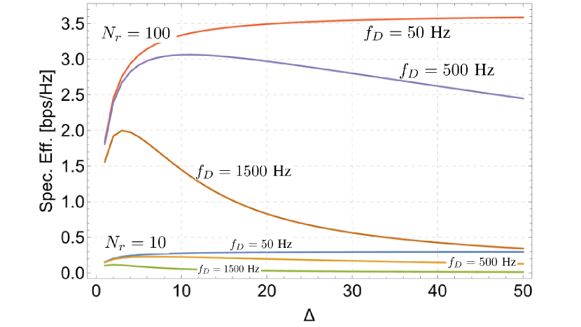
Figure 2: Spectral efficiency as a function of frame size ($\Delta$) with maximum Doppler frequency $f_{D}=50,500,1500$ Hz with $N_{r}=10$ (lower three curves) and $N_{r}=100$ (upper three curves). At higher maximum Doppler frequency, the optimum frame size is smaller than at low Doppler frequency.

Figure 2 shows the achieved spectral efficiency averaged over the data slots $i=1\dots\Delta$, that is averaged over the data slots of a frame of size $\Delta+1$. Short frames imply that the pilot overhead is relatively large, which results in poor spectral efficiency. On the other hand, too large frames (that is when $\Delta$ is too large) make the channel estimation quality in the "middle" time slots poor, since for these time slots both available channel estimates $\mathbf{\hat{h}}(0)$ and $\mathbf{\hat{h}}(\Delta+1)$ convey little useful information, especially at high Doppler frequencies when the channel ages rapidly. Indeed, as seen in Figure 2, the frame size has a large impact on the achievable spectral efficiency, suggesting that the optimum frame size depends critically on the Doppler frequency. As we can see, the spectral efficiency as a function of the frame size is in general neither monotone nor concave, and is hence hard to optimize.

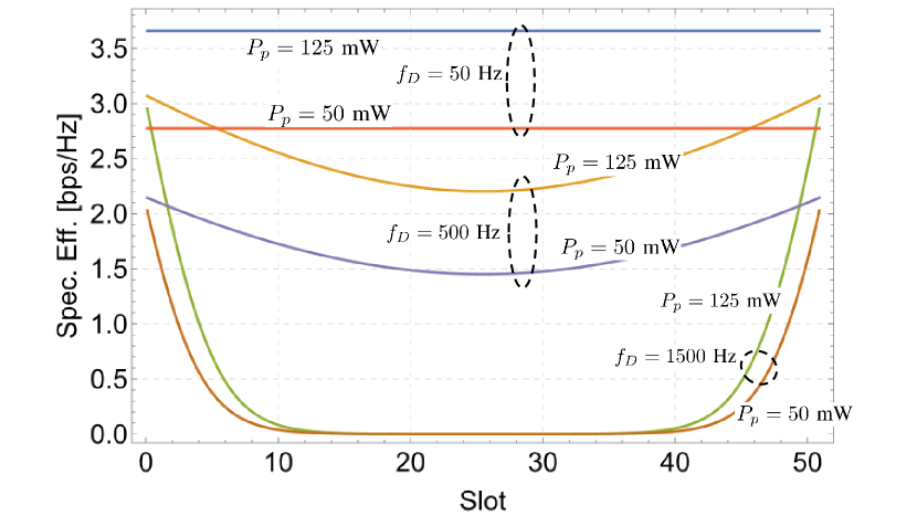
Figure 3: Spectral efficiency for each data slot $i=1\dots\Delta$ when the frame size is kept fixed ($\Delta=50$). At high maximum Doppler frequency, the spectral efficiency is low at the "middle" slot, while at low maximum Doppler the spectral efficiency reaches its maximum at the middle slots.

Figure 3 shows the spectral efficiency for each data slot $i=1\dots\Delta$ within a frame of size $\Delta=50$. At lower Doppler frequencies, that is when the channel fades relatively slowly, the channel state information acquisition in the middle slots benefits from using the estimates at $i=0$ and $i=\Delta+1$, and making an MMSE interpolation of the channel coefficients as proposed in Lemma 1. However, at a high Doppler frequency, the channel state in the middle data slots are weakly correlated with the channel estimates $\mathbf{\hat{h}}(0)$ and $\mathbf{\hat{h}}(\Delta+1)$, which makes the MMSE channel estimation error in Corollary 1 large. This insight suggests that in such cases, the optimum frame size is much less than when the Doppler frequency is low.

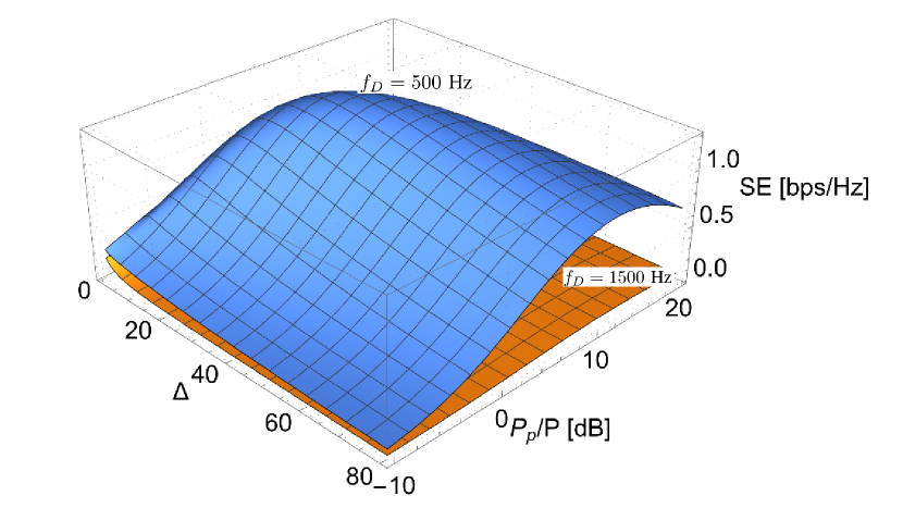
Figure 4: Spectral efficiency as a function of the pilot/data power ratio and the frame size for maximum Doppler frequency $f_{D}=500$ Hz and $f_{D}=1500$ Hz when $N_{r}=10$. In both cases, the spectral efficiency depends heavily on the employed pilot power and pilot spacing (frame size).

The average spectral efficiency as a function of the pilot/data power ratio and the frame size is shown in Figure 4. This figure clearly shows that setting the proper frame size and tuning the pilot/data power ratio are both important to maximize the average spectral efficiency of the system. The optimal frame size and power configuration are different for different Doppler frequencies, which in turn emphasizes the importance of accurate Doppler frequency estimates.

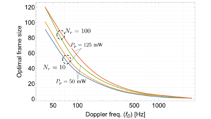
Figure 5: Optimal frame size as a function of the maximum Doppler frequency for different values of the employed pilot power ($P_{p}=50$ mW and $P_{p}=125$ mW) when the BS is equipped with $N_{r}=10$ and $N_{r}=100$ receive antennas.

The optimal frame size as a function of the maximum Doppler frequency is shown in Figure 5. The optimal frame size decreases rapidly, as the Doppler effect increases. As this figure shows, a much larger frame size is optimal when the number of antennas is high and the MS uses high pilot power to achieve a high pilot signal-to-noise ratio (SNR).

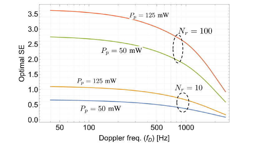
Figure 6: Optimal spectral efficiency as a function of the maximum Doppler frequency, that is the spectral efficiency when using the optimal frame size as shown in Figure 5.

Figure 6 shows the achieved spectral efficiency when the frame size is set optimally, as a function of the maximum Doppler frequency. At $f_{D}=500$ Hz, for example, when the optimal frame size is 8 (see also Figures 2 and 5), the achieved spectral efficiency when using $N_{r}=10$ antennas is a bit below 1 bps/Hz. We can see that setting the optimal frame size is indeed important, because it helps to make the achievable spectral efficiency quite robust with respect to even a significant increase in the Doppler frequency.

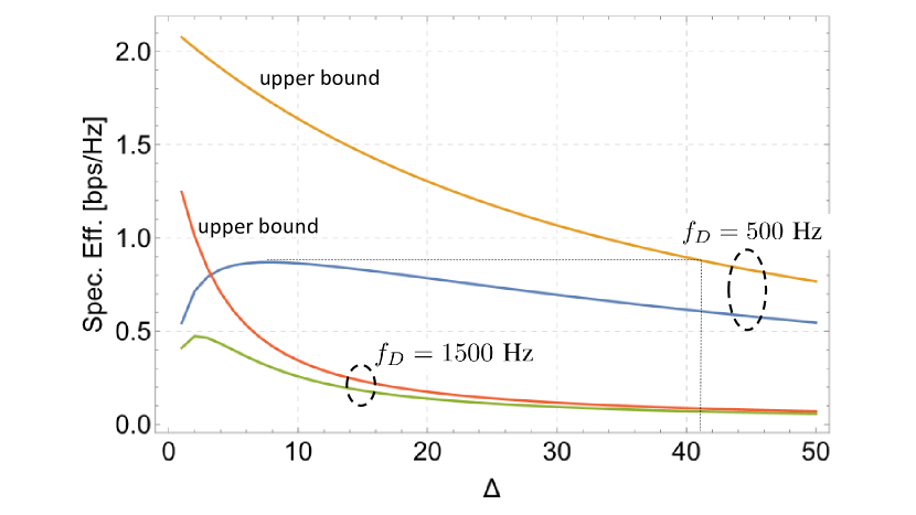
Figure 7: Upper bounding the achievable spectral efficiency as a function of the frame size ($\Delta$) at $f_{D}=500$ Hz and $f_{D}=1500$ Hz. Note that the upper bound is monotonically decreasing, which helps to limit the search space for the optimum frame size.

Figure 7 illustrates the upper bounds on spectral efficiency as a function of the frame size for different Doppler frequencies. Recall from Figure 2 that the spectral efficiency of the system is a non-concave function of the frame size. Therefore, limiting the possible frame sizes that can optimize spectral efficiency is useful, which can be achieved by the upper bounds shown in the figure. Since the upper bound is monotonically decreasing, finding a point of the spectral efficiency curve (see the curve marked with $f_{D}=500$ Hz and its upper bounding curve) with a negative derivative helps to find the range of possible frame sizes that maximize spectral efficiency. For $f_{D}=500$ Hz, as illustrated in the figure, larger frame sizes than $\Delta=41$ would lead to a lower upper bound than the spectral efficiency achieved at $\Delta=7$. Therefore, when searching for the optimal $\Delta$, once we found that the spectral efficiency at $\Delta=8$ is less than at $\Delta=7$ (negative derivative), the search space is limited to $(7,41)$.

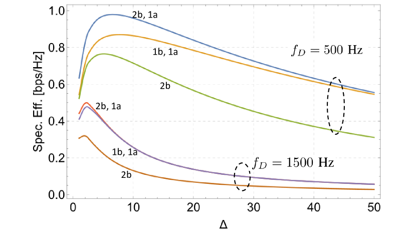
Figure 8: Spectral efficiency in each time slot for $f_{D}=500$ Hz and $f_{D}=1500$ Hz, when using 1 or 2 pilot symbols preceding that time slot and 0 or 1 pilot symbols after that time slot for channel estimation. Three combinations of these channel estimation schemes are denoted as "2b, 1a", "1b, 1a" and "2b", where "b" refers to utilizing the pilot symbols sent before and "a" refers to utilizing the pilot symbol sent after time slot $i$.

Figure 8 compares the average spectral efficiency when the system uses different number of pilot signals to estimate the channel state for each data slot within the frame. Specifically, three schemes are compared:

• 2 before, 1 after (2b, 1a): Three channel estimates using the pilot signals at the beginning of the current frame and the preceding frame and at the end of the current frame are used to interpolate the channel state at every data slot in the current frame.

• 1 before, 1 after (1b, 1a): The two neighboring pilot signals (that is in the beginning and at the end of the current frame) are used.

• 2 before (2b): The pilot signals at the beginning of the current and preceding frames are used. This scheme has an advantage over the previous schemes in that decoding the received data symbols is possible "on the fly" without having to await the upcoming pilot signal at the end of the current frame.

Notice that the "1b, 1a" scheme outperforms the "2b" scheme, because the channel estimation instances are closer to the data transmission instance in time. Furthermore, the "2b, 1a" scheme further improves the SE performance, although this improvement over the "1b, 1a" scheme is marginal. More importantly, we can observe that the optimal pilot spacing is similar in these three schemes, but depends heavily on the Doppler frequency.

Figure 9: Spectral efficiency as a function of the frame size $\Delta$ when the receiver under or overestimates the actual Doppler frequency of the channel ($f_{D}=200$ Hz and $f_{D}=500$ Hz). Overestimating the actual Doppler frequency causes significant spectral efficiency degradation for most frame sizes.

Finally, Figure 9 examines the negative impact of Doppler frequency estimation errors when the Doppler frequency of the channel is under or overestimated. The figure shows the spectral efficiency as a function of the frame size for the cases when $f_{D}=200$ Hz and $f_{D}=500$ Hz. For both cases, the Doppler frequency is either correctly estimated or overestimated (to $5f_{D}$) or underestimated (to $0.2f_{D}$). On the one hand, this figure clearly illustrates the performance degradation in terms of average spectral efficiency when the receiver underestimates or overestimates the maximum Doppler frequency. On the other hand, when using the optimal frame size, the spectral efficiency performance of these schemes are rather similar in most cases.

VIII Conclusions

This paper investigated the fundamental trade-off between using resources in the time domain for pilot signals and data signals in the uplink of MU-MIMO systems operating over fast fading wireless channels that age between subsequent pilot signals. While previous works indicated that when the autocorrelation coefficient between subsequent channel realization instances in discrete time is high, both the channel estimation and the MU-MIMO receiver can take advantage of the memoryful property of the channel in the time domain. However, previous works do not answer the question how often the channel should be observed and estimated such that the subsequent channel samples are sufficiently correlated while taking into account that pilot signals do not carry information bearing symbols and degrade the overall spectral efficiency. To find the optimal pilot spacing, we first established the deterministic equivalent of the achievable SINR and the associated overall spectral efficiency of the MU-MIMO system. We then used some useful properties of an upper bound of this spectral efficiency, which allowed us to limit the search space for the optimal pilot spacing ($\Delta$). The numerical results indicate that the optimal pilot spacing is sensitive to the Doppler frequency of the channel and that proper pilot spacing has a significant impact on the achievable spectral efficiency.

Appendix A Proof of Lemma 4

Proof.

Notice that

$$\mathbf{M}(\Delta,i) =\underbrace{\begin{bmatrix}1&e^{2qi}&e^{4qi}\\ {(e^{2qi})}^{*}&1&e^{2qi}\\ {(e^{4qi})}^{*}&{(e^{2qi})}^{*}&1\\ \end{bmatrix}}_{\triangleq\mathbf{M}_{3}(\Delta,i)}\otimes\mathbf{C},$$ (64)

and the eigenvalues of $\mathbf{M}_{3}(\Delta,i)$ are:

$$\lambda_{1}(i) =1-a^{2i};$$

$$\lambda_{2}(i) =\frac{1}{2}\left(2+a^{2i}-a^{i}\sqrt{8+a^{2i}}\right);$$

$$\lambda_{3}(i) =\frac{1}{2}\left(2+a^{2i}+a^{i}\sqrt{8+a^{2i}}\right),$$

where $0<a<1$. For all $i\geq 1$ the smallest eigenvalue is $\lambda_{2}(i)$, which monotone increases with $i$. That is, $\min_{i\geq 1,j\in\{1,2,3\}}\lambda_{j}(i)=\lambda_{2}(1)$.

Let

$$\mathbf{M}^{(u)}(\Delta) \triangleq\underbrace{\begin{bmatrix}\eta&0&0\\ 0&\eta&0\\ 0&0&\eta\\ \end{bmatrix}}_{\triangleq\mathbf{M}^{(u)}_{3}(\Delta)}\otimes\mathbf{C}.$$ (65)

When $\eta<\lambda_{2}(1)$ according to (42), we have

$$\mathbf{M}_{3}^{(u)}(\Delta)\preceq\mathbf{M}_{3}(\Delta).$$ (66)

Utilizing that the spectrum of a Kronecker product $\sigma(\mathbf{A}\otimes\mathbf{B})$ is [34]

$$\sigma(\mathbf{A}\otimes\mathbf{B}) =\{\,\mu_{A}\mu_{B}\mid\mu_{A}\in\sigma(\mathbf{A}),\mu_{B}\in\sigma(\mathbf{B})\,\},$$ (67)

for $\forall i\geq 1$, we further have

$$\mathbf{M}^{(u)}(\Delta)\preceq\mathbf{M}(\Delta,i),$$ (68)

which implies

$$\big{(}\mathbf{M}^{(u)}(\Delta)+\mathbf{\Sigma}_{3}\big{)}^{-1}\succeq\big{(}\mathbf{M}(\Delta,i)+\mathbf{\Sigma}_{3}\big{)}^{-1},$$ (69)

according to (44). The statement of the lemma comes from (69) using (45), $\mathbf{M}^{(u)}(\Delta)=\eta\mathbf{I}_{3}\otimes\mathbf{C}$, and noting that

$$\mathbf{E}(\Delta,i)\big{(}\mathbf{M}^{(u)}(\Delta)+\mathbf{\Sigma}_{3}\big{)}^{-1}\mathbf{E}(\Delta,i)^{H}$$

$$=\mathbf{E}(\Delta,i)\begin{bmatrix}\eta\mathbf{C}+\bm{\Sigma}&0&0\\ 0&\eta\mathbf{C}+\bm{\Sigma}&0\\ 0&0&\eta\mathbf{C}+\bm{\Sigma}\\ \end{bmatrix}^{-1}\mathbf{E}(\Delta,i)^{H}$$

$$=\mathbf{R}(\Delta\!+\!1\!+\!i)(\eta\mathbf{C}+\bm{\Sigma})^{-1}\mathbf{R}(\Delta\!+\!1\!+\!i)^{H}$$

$$\leavevmode\nobreak\ \leavevmode\nobreak\ \leavevmode\nobreak\ +\mathbf{R}(i)(\eta\mathbf{C}+\bm{\Sigma})^{-1}\mathbf{R}(i)^{H}$$

$$\leavevmode\nobreak\ \leavevmode\nobreak\ \leavevmode\nobreak\ +\mathbf{R}(\Delta\!+\!1\!-\!i)(\eta\mathbf{C}+\bm{\Sigma})^{-1}\mathbf{R}(\Delta\!+\!1\!-\!i)^{H}$$

$$=\rho(\Delta,i)\mathbf{C}\left(\eta\mathbf{C}+\bm{\Sigma}\right)^{-1}\mathbf{C},$$ (70)

where $\mathbf{R}(i)$ and $\rho(\Delta,i)$ are defined in (36) and (41). ∎

Appendix B Proof of Lemma 5

Proof.

$$\bar{\gamma}(\Delta,i)$$

$$=\mathds{E}\left(\textup{tr}\left(\bm{\Phi}(\Delta,i)\left(\sum_{k=2}^{K}\mathbf{b}_{l}(\Delta,i)\mathbf{b}_{l}^{H}(\Delta,i)+\bm{\beta}(\Delta,i)\right)^{-1}\right)\right)$$

$$=\int\limits_{\mathbf{v}_{2}\in\mathbb{R}^{N_{r}}}\!\!\!\ldots\!\!\!\int\limits_{\mathbf{v}_{K}\in\mathbb{R}^{N_{r}}}\prod_{k=2}^{K}Pr(\mathbf{b}_{l}(\Delta,i)=\mathbf{v}_{l})$$

$$\leavevmode\nobreak\ \leavevmode\nobreak\ \leavevmode\nobreak\ \leavevmode\nobreak\ \leavevmode\nobreak\ \leavevmode\nobreak\ \cdot\textup{tr}\left(\bm{\Phi}(\Delta,i)\left(\sum_{k=2}^{K}\mathbf{v}_{l}\mathbf{v}_{l}^{H}+\bm{\beta}(\Delta,i)\right)^{-1}\right)d\mathbf{v}_{K}\ldots d\mathbf{v}_{2}$$

$$\leq\int\limits_{\mathbf{v}_{2}\in\mathbb{R}^{N_{r}}}\int\limits_{\mathbf{v}_{K}\in\mathbb{R}^{N_{r}}}\prod_{k=2}^{K}Pr(\mathbf{b}_{l}(\Delta,i)=\mathbf{v}_{l})$$

$$\leavevmode\nobreak\ \leavevmode\nobreak\ \leavevmode\nobreak\ \leavevmode\nobreak\ \leavevmode\nobreak\ \leavevmode\nobreak\ \leavevmode\nobreak\ \leavevmode\nobreak\ \leavevmode\nobreak\ \leavevmode\nobreak\ \leavevmode\nobreak\ \leavevmode\nobreak\ \leavevmode\nobreak\ \leavevmode\nobreak\ \leavevmode\nobreak\ \leavevmode\nobreak\ \leavevmode\nobreak\ \leavevmode\nobreak\ \cdot\textup{tr}\left(\bm{\Phi}(\Delta,i)\bm{\beta}(\Delta,i)^{-1}\right)d\mathbf{v}_{K}\ldots d\mathbf{v}_{2}$$

$$=\textup{tr}\left(\bm{\Phi}(\Delta,i)\bm{\beta}(\Delta,i)^{-1}\right),$$

where we used that $\sum_{l=2}^{K}\mathbf{v}_{l}\mathbf{v}_{l}^{H}$ is a positive definite matrix, $\sum_{l=2}^{K}\mathbf{v}_{l}\mathbf{v}_{l}^{H}+\bm{\beta}(\Delta,i)\succeq\bm{\beta}(\Delta,i)$ and Lemma 3. ∎

Appendix C Proof of Proposition 2

Proof.

To prove monotonicity in $\rho$ first notice that

$$\rho(\Delta_{1},i_{1})>\rho(\Delta_{2},i_{2})\Rightarrow\mathbf{Z}^{(u)}(\Delta_{1},i_{1})\preceq\mathbf{Z}^{(u)}(\Delta_{2},i_{2}),$$

$$\rho(\Delta_{1},i_{1})>\rho(\Delta_{2},i_{2})\Rightarrow\bm{\Phi}^{(u)}(\Delta_{1},i_{1})\succeq\bm{\Phi}^{(u)}(\Delta_{2},i_{2}).$$

and so

$$\rho(\Delta_{1},i_{1})>\rho(\Delta_{2},i_{2})$$

$$\Downarrow$$

$$\begin{aligned} &\bm{\Phi}^{(u)}(\Delta_{1},i_{1})\left(\sum_{l=1}^{K}\alpha_{l}^{2}P_{l}\mathbf{Z}^{(u)}_{l}(\Delta_{1},i_{1})+\sigma_{d}^{2}\mathbf{I}_{N_{r}}\right)^{-1}\\ &\leavevmode\nobreak\ \leavevmode\nobreak\ \succeq\bm{\Phi}^{(u)}(\Delta_{2},i_{2})\left(\sum_{l=1}^{K}\alpha_{l}^{2}P_{l}\mathbf{Z}^{(u)}_{l}(\Delta_{2},i_{2})+\sigma_{d}^{2}\mathbf{I}_{N_{r}}\right)^{-1}\end{aligned}$$

$$\Downarrow$$

$$\begin{aligned} &\textup{tr}\left(\bm{\Phi}^{(u)}(\Delta_{1},i_{1})\left(\sum_{l=1}^{K}\alpha_{l}^{2}P_{l}\mathbf{Z}^{(u)}_{l}(\Delta_{1},i_{1})+\sigma_{d}^{2}\mathbf{I}_{N_{r}}\right)^{-1}\right)\\ &\geq\textup{tr}\!\left(\!\bm{\Phi}^{(u)}(\Delta_{2},i_{2})\left(\sum_{l=1}^{K}\alpha_{l}^{2}P_{l}\mathbf{Z}^{(u)}_{l}(\Delta_{2},i_{2})+\sigma_{d}^{2}\mathbf{I}_{N_{r}}\!\right)^{\!\!-1}\right)\end{aligned}$$

$$\Downarrow$$

$$\bar{\gamma}^{(u)}(\Delta_{1},i_{1})\geq\bar{\gamma}^{(u)}(\Delta_{2},i_{2}).$$

Finally to prove convergence to 0 notice that

$$\rho(\Delta,i)\rightarrow 0 \Rightarrow\mathbf{Z}^{(u)}(\Delta_{1},i_{1})\rightarrow\mathbf{C},$$

$$\rho(\Delta,i)\rightarrow 0 \Rightarrow\bm{\Phi}^{(u)}(\Delta_{1},i_{1})\rightarrow\mathbf{0}.$$

And so, when $\rho(\Delta,i)\rightarrow 0$ we have

$$\bar{\gamma}^{(u)} (\Delta,i)=$$

$$\textup{tr}\left(\bm{\Phi}^{(u)}(\Delta,i)\left(\sum_{l=1}^{K}\alpha_{l}^{2}P_{l}\mathbf{Z}^{(u)}_{l}(\Delta,i)+\sigma_{d}^{2}\mathbf{I}_{N_{r}}\right)^{-1}\right)$$

$$\stackrel{{\scriptstyle\rho(\Delta,i)\rightarrow 0}}{{\rightarrow}}\textup{tr}\left(\mathbf{0}\left(\sum_{l=1}^{K}\alpha_{l}^{2}P_{l}\mathbf{C}+\sigma_{d}^{2}\mathbf{I}_{N_{r}}\right)^{-1}\right)=0.$$

∎

Appendix D Proof of Proposition 3

Proof.

From Theorem 1 and (52) the inequality follows. For monotonicity, notice that $\rho_{k}(\Delta+1,i)<\rho_{k}(\Delta,i)$ and $\rho_{k}(\Delta+1,i+1)<\rho_{k}(\Delta,i)$. Since by Proposition 2 the upper bound of the SINR is increasing with $\rho_{k}$ we have

$$\bar{\gamma}_{k}^{(u)}(\Delta+1,i) \leq\bar{\gamma}_{k}^{(u)}(\Delta,i)$$

$$\bar{\gamma}_{k}^{(u)}(\Delta+1,i+1) \leq\bar{\gamma}_{k}^{(u)}(\Delta,i),$$ (71)

from which it follows that

$$\log\big{(}1+\bar{\gamma}_{k}^{(u)}(\Delta+1,i)\big{)} \leq\log\big{(}1+\bar{\gamma}_{k}^{(u)}(\Delta,i)\big{)}$$ (72)

$$\log\big{(}1+\bar{\gamma}_{k}^{(u)}(\Delta+1,i+1)\big{)} \leq\log\big{(}1+\bar{\gamma}^{(u)}(\Delta,i)\big{)}.$$ (73)

Let $\ell=\arg\min_{i}\bar{\gamma}_{k}^{(u)}(\Delta+1,i)$, we then have

$$\frac{1}{\Delta+1}\times\sum_{i=1}^{\Delta+1}\log\big{(}1+\bar{\gamma}_{k}^{(u)}(\Delta+1,i)\big{)}$$

$$\leq\frac{1}{\Delta}\times\left(\sum_{i=1}^{\ell-1}\log\big{(}1+\bar{\gamma}_{k}^{(u)}(\Delta+1,i)\big{)}\right.$$

$$\leavevmode\nobreak\ \leavevmode\nobreak\ \leavevmode\nobreak\ \leavevmode\nobreak\ \leavevmode\nobreak\ \leavevmode\nobreak\ \leavevmode\nobreak\ \leavevmode\nobreak\ \leavevmode\nobreak\ \leavevmode\nobreak\ \leavevmode\nobreak\ \leavevmode\nobreak\ \leavevmode\nobreak\ \leavevmode\nobreak\ \leavevmode\nobreak\ \leavevmode\nobreak\ \leavevmode\nobreak\ \leavevmode\nobreak\ \leavevmode\nobreak\ \leavevmode\nobreak\ +\left.\sum_{i=\ell+1}^{\Delta+1}\log\big{(}1+\bar{\gamma}_{k}^{(u)}(\Delta+1,i)\big{)}\right),$$ (74)

since on the right hand side we are removing the smallest term before calculating the mean. Invoking (72) and (73) on the first and second sum, respectively, it follows that

$$\frac{1}{\Delta+1}\times\sum_{i=1}^{\Delta+1}\log\big{(}1+\bar{\gamma}_{k}^{(u)}(\Delta+1,i)\big{)}$$

$$\leq\frac{1}{\Delta+1}\times\left(\sum_{i=1}^{\ell-1}\log\big{(}1+\bar{\gamma}_{k}^{(u)}(\Delta,i)\big{)}\right.$$

$$\leavevmode\nobreak\ \leavevmode\nobreak\ \leavevmode\nobreak\ \leavevmode\nobreak\ \leavevmode\nobreak\ \leavevmode\nobreak\ \leavevmode\nobreak\ \leavevmode\nobreak\ \leavevmode\nobreak\ \leavevmode\nobreak\ \leavevmode\nobreak\ \leavevmode\nobreak\ \leavevmode\nobreak\ \leavevmode\nobreak\ \leavevmode\nobreak\ \leavevmode\nobreak\ \leavevmode\nobreak\ \leavevmode\nobreak\ \leavevmode\nobreak\ \leavevmode\nobreak\ \leavevmode\nobreak\ +\left.\sum_{i=\ell}^{\Delta}\log\big{(}1+\bar{\gamma}_{k}^{(u)}(\Delta,i)\big{)}\right)$$

$$=\frac{1}{\Delta}\times\sum_{i=1}^{\Delta}\log\big{(}1+\bar{\gamma}_{k}^{(u)}(\Delta,i)\big{)}.$$ (75)

From which it follows that

$$\textup{SE}_{k}^{(u)}(\Delta+1)=\frac{\sum_{i=1}^{\Delta+1}\log\big{(}1+\bar{\gamma}_{k}^{(u)}(\Delta+1,i)\big{)}}{\Delta+1}$$

$$\leavevmode\nobreak\ \leavevmode\nobreak\ \leavevmode\nobreak\ \leavevmode\nobreak\ \leavevmode\nobreak\ \leq\frac{\sum_{i=1}^{\Delta}\log\big{(}1+\bar{\gamma}_{k}^{(u)}(\Delta,i)\big{)}}{\Delta}=\textup{SE}_{k}^{(u)}(\Delta),$$ (76)

that is $\textup{SE}_{k}^{(u)}(\Delta)$ is decreasing in $\Delta$.

To prove convergence to zero, recall from Proposition 2 that $\partial\bar{\gamma}_{k}^{(u)}(\Delta,i)/\partial\rho_{k}(\Delta,i)\geq 0$ and

$$\rho_{k}(\Delta,i)\rightarrow 0 \Rightarrow\bar{\gamma}_{k}^{(u)}(\Delta,i)\rightarrow 0$$

$$\Rightarrow\log\big{(}1+\bar{\gamma}_{k}^{(u)}(\Delta,i)\big{)}\rightarrow 0,$$ (77)

where

$$\rho_{k}(\Delta,i)=e^{2\bar{q}_{k}(\Delta+1+i)}+e^{2\bar{q}_{k}i}+e^{2\bar{q}_{k}(\Delta+1-i)}.$$

We show that for any $\varepsilon>0$, there is some $M$ such that

$$\textup{SE}^{(u)}(M)<\varepsilon.$$ (78)

Due to $\bar{q}_{k}<0$, we have $\rho_{k}(\Delta,i)<\rho_{k}(1,1)$, which implies

$$\log\big{(}1+\bar{\gamma}_{k}^{(u)}(\Delta,i)\big{)}<\log\big{(}1+\bar{\gamma}_{k}^{(u)}(1,1)\big{)},$$ (79)

for all $\Delta$ and $i$. Let $A\triangleq\log\big{(}1+\bar{\gamma}_{k}^{(u)}(1,1)\big{)}$ and $N$ such that $N\varepsilon-2A>0$, and set

$$\epsilon\triangleq\frac{N\varepsilon-2A}{N-2}.$$ (80)

Since $\bar{q}_{k}<0$, we have

$$\rho_{k}(\Delta,i) <3\max(e^{2\bar{q}_{k}(\Delta+1+i)},e^{2\bar{q}_{k}i},e^{2\bar{q}_{k}(\Delta+1-i)})$$

$$=3e^{2\bar{q}_{k}\min(\Delta+1+i,i,\Delta+1-i)},$$

and it follows that for $\frac{\Delta}{N}\leq i\leq\frac{(N-1)\Delta}{N}$

$$\rho_{k}(\Delta,i)<3e^{2\bar{q}_{k}\frac{\Delta}{N}}.$$ (81)

Notice that by equation (77) we can choose some large $M$, such that

$$\frac{M}{N}\leq i\leq\frac{(N-1)M}{N}\Rightarrow\log(1+\bar{\gamma}_{k}^{(u)}(M,i))<\epsilon.$$ (82)

We can now show that when $M=\Delta$, then $\textup{SE}_{k}^{(u)}(\Delta)<\varepsilon$. To this end, we split up the sum in the numerator of (76), that is $\sum_{i=1}^{\Delta}\log(1+\bar{\gamma}^{(u)}(\Delta,i))$, into three terms, and bound the first and third terms using the general upper bound $A$, and the middle term by $\epsilon$:

$$\textup{SE}_{k}^{(u)}(\Delta) =\frac{\sum_{i=1}^{\Delta}\log(1+\bar{\gamma}^{(u)}(\Delta,i))}{\Delta}$$

$$=\frac{\sum_{i=1}^{\Delta/N}\log(1+\bar{\gamma}^{(u)}(\Delta,i))}{\Delta}$$

$$\leavevmode\nobreak\ \leavevmode\nobreak\ \leavevmode\nobreak\ \leavevmode\nobreak\ +\frac{\sum_{i=\Delta/N+1}^{(N-1)\Delta/N}\log(1+\bar{\gamma}^{(u)}(\Delta,i))}{\Delta}$$

$$\leavevmode\nobreak\ \leavevmode\nobreak\ \leavevmode\nobreak\ \leavevmode\nobreak\ +\frac{\sum_{i=(N-1)\Delta/N+1}^{\Delta}\log(1+\bar{\gamma}^{(u)}(\Delta,i))}{\Delta}$$

$$<\frac{(\Delta/N)A}{\Delta}+\frac{((N-2)\Delta/N)\epsilon}{\Delta}+\frac{(\Delta/N)A}{\Delta}$$

$$=\frac{2A+(N-2)\epsilon}{N}=\varepsilon,$$ (83)

where the last equation is due to the definition of $\epsilon$ in (80), which completes the proof. ∎

References

- [1] M. Yan and D. Rao, “Performance of an array receiver with a Kalman channel predictor for fast Rayleigh flat fading environments,” IEEE Journal on Selected Areas in Communications, vol. 6, no. 6, pp. 1164–1172, 2001.
- [2] Y. Zhang, S. B. Gelfand, and M. P. Fitz, “Soft-output demodulation on frequency-selective Rayleigh fading channels uing AR channel models,” IEEE Transactions on Communications, vol. 55, no. 10, pp. 1929–1939, Oct. 2007.
- [3] H. Abeida, “Data-aided SNR estimation in time-variant Rayleigh fading channels,” IEEE Transactions on Signal Processing, vol. 58, no. 11, pp. 5496–5507, Nov. 2010.
- [4] H. Hijazi and L. Ros, “Joint data QR-detection and Kalman estimation for OFDM time-varying Rayleigh channel complex gains,” IEEE Transactions on Communications, vol. 58, no. 1, pp. 170–177, Jan. 2010.
- [5] S. Ghandour-Haidar, L. Ros, and J.-M. Brossier, “On the use of first-order autorgegressive modeling for Rayleigh flat fading channel estimation with Kalman filter,” Elsevier Signal Processing, no. 92, pp. 601–606, 2012.
- [6] K. T. Truong and R. W. Heath, “Effects of channel aging in massive MIMO systems,” Journal of Communications and Networks, vol. 15, no. 4, pp. 338–351, 2013.
- [7] C. Kong, C. Zhong, A. K. Papazafeiropoulos, M. Matthaiou, and Z. Zhang, “Sum-rate and power scaling of massive MIMO systems with channel aging,” IEEE Transactions on Communications, vol. 63, no. 12, pp. 4879–4893, 2015.
- [8] L.-K. Chiu and S.-H. Wu, “An effective approach to evaluate the training and modeling efficacy in MIMO time-varying fading channels,” IEEE Transactions on Communications, vol. 63, no. 1, pp. 140–155, 2015.
- [9] S. Kashyap, C. Mollén, E. Björnson, and E. G. Larsson, “Performance analysis of (TDD) massive MIMO with Kalman channel prediction,” in IEEE International Conference on Acoustics, Speech and Signal Processing (ICASSP). New Orleans, LA, USA: IEEEE, Mar. 2017.
- [10] H. Kim, S. Kim, H. Lee, C. Jang, Y. Choi, and J. Choi, “Massive MIMO channel prediction: Kalman filtering vs. machine learning,” IEEE Transactions on Communications, pp. 1–1, 2020, early access.
- [11] J. Yuan, H. Q. Ngo, and M. Matthaiou, “Machine learning-based channel prediction in massive MIMO with channel aging,” IEEE Transactions on Wireless Communications, vol. 19, no. 5, pp. 2960–2973, 2020.
- [12] G. Fodor, S. Fodor, and M. Telek, “Performance analysis of a linear MMSE receiver in time-variant rayleigh fading channels,” IEEE Transactions on Communications, vol. 69, no. 6, pp. 4098–4112, 2021.
- [13] R. Couillet, J. Hoydis, and M. Debbah, “Random beamforming over quasi-static and fading channels: A deterministic equivalent approach,” IEEE Transactions on Information Theory, vol. 58, no. 10, pp. 6392–6425, 2012.
- [14] C. Wen, G. Pan, K. Wong, M. Guo, and J. Chen, “A deterministic equivalent for the analysis of non-Gaussian correlated MIMO multiple access channels,” IEEE Transactions on Information Theory, vol. 59, no. 1, pp. 329–352, 2013.
- [15] J. Hoydis, S. T. Brink, and M. Debbah, “Massive MIMO in the UL/DL of cellular networks: How many antennas do we need ?” IEEE Journal on Selected Areas in Communications, vol. 31, no. 2, pp. 160–171, Feb. 2013.
- [16] R. K. Mallik, M. R. Bhatnagar, and S. P. Dash, “Fractional pilot duration optimization for SIMO in Rayleigh fading with MPSK and imperfect CSI,” IEEE Transactions on Communications, vol. 66, no. 4, pp. 1732–1744, 2018.
- [17] L. Hanlen and A. Grant, “Capacity analysis of correlated MIMO channels,” IEEE Transactions on Information Theory, vol. 58, no. 11, pp. 6773–6787, 2012.
- [18] A. Mahmoudi and M. Karimi, “Inverse filtering based method for estimation of noisy autoregressive signals,” Signal Processing, vol. 91, no. 7, pp. 1659–1664, 2011.
- [19] Y. Xia and W. X. Zheng, “Novel parameter estimation of autoregressive signals in the presence of noise,” Automatica, vol. 62, pp. 98–105, 2015.
- [20] M. Esfandiari, S. A. Vorobyov, and M. Karimi, “New estimation methods for autoregressive process in the presence of white observation noise,” Signal Porcessing (Elsevier), vol. 2020, no. 171, pp. 10 780–10 790, 2020.
- [21] Y. R. Zheng and C. Xiao, “Simulation models with correct statistical properties for Rayleigh fading channels,” IEEE Transactions on Communications, vol. 51, no. 6, pp. 920–928, 2003.
- [22] C.-X. Wang, M. Ptzold, and Q. Yao, “Stochastic modeling and simulation offrequency-correlated wideband fading channels,” IEEE Transactions on Vehicular Technology, vol. 56, no. 3, pp. 1050–1063, May 2007.
- [23] M. McGuire and M. Sima, “Low-order Kalman filters for channel estimation,” in IEEE Pacific Rim Conference on Communications, Computers and Signal Processing (PACRIM), Victoria, BC, Canada, Aug. 2005, pp. 352–355.
- [24] W. X. Zheng, “Fast identification of autoregressive signals from noisy observations,” IEEE Transactions on Circuits and Systems, vol. 52, no. 1, pp. 43–48, Jan. 2005.
- [25] S. Savazzi and U. Spagnolini, “On the pilot spacing constraints for continuous time-varying fading channels,” IEEE Transactions on Communications, vol. 57, no. 11, pp. 3209–3213, 2009.
- [26] ——, “Optimizing training lengths and training intervals in time-varying fading channels,” IEEE Transactions on Signal Processing, vol. 57, no. 3, pp. 1098–1112, 2009.
- [27] S. Akin and M. C. Gursoy, “Training optimization for Gauss-Markov Rayleigh fading channels,” in 2007 IEEE International Conference on Communications, 2007, pp. 5999–6004.
- [28] K. E. Baddour and N. C. Beaulieu, “Autoregressive modeling for fading channel simulation,” IEEE Trans. Wirel. Commun., vol. 4, no. 4, pp. 1650–1662, 2005.
- [29] G. Fodor, S. Fodor, and M. Telek, “On the achievable SINR in MU-MIMO systems operating in time-varying Rayleigh fading,” IEEE Transactions on Communications (Early Access), 2022, DoI: 10.1109/TCOMM.2021.3126760.
- [30] S. Wagner, R. Couillet, M. Debbah, and D. T. M. Slock, “Large system analysis of linear precoding in correlated MISO broadcast channels under limited feedback,” IEEE Transactions on Information Theory, vol. 58, no. 7, pp. 4509–4537, 2012.
- [31] C.-X. Wang and M. Patzold, “Efficient simulation of multiple cross-correlated rayleigh fading channels,” in 14th IEEE Proceedings on Personal, Indoor and Mobile Radio Communications, 2003. PIMRC 2003., vol. 2, 2003, pp. 1526–1530 vol.2.
- [32] R. A. Horn and C. R. Johnson, Matrix Analysis (2nd ed.). Cambridge University Press, 2013.
- [33] A. A. Zaidi, R. Baldemair, H. Tullberg, H. Bjorkegren, L. Sundstrom, J. Medbo, C. Kilinc, and I. Da Silva, “Waveform and numerology to support 5g services and requirements,” IEEE Communications Magazine, vol. 54, no. 11, pp. 90–98, 2016.
- [34] R. A. Horn and C. R. Johnson, Topics in Matrix Analysis. Cambridge University Press, 1991.