Green Routing Game: Strategic Logistical Planning
using Mixed Fleets of ICEVs and EVs
Abstract
This paper introduces a “green” routing game between multiple logistic operators (players), each owning a mixed fleet of internal combustion engine vehicle (ICEV) and electric vehicle (EV) trucks. Each player faces the cost of delayed delivery (due to charging requirements of EVs) and a pollution cost levied on the ICEVs. This cost structure models: 1) limited battery capacity of EVs and their charging requirement; 2) shared nature of charging facilities; 3) pollution cost levied by regulatory agency on the use of ICEVs. We characterize Nash equilibria of this game and derive a condition for its uniqueness. We also use the gradient projection method to compute this equilibrium in a distributed manner. Our equilibrium analysis is useful to analyze the trade-off faced by players in incurring higher delay due to congestion at charging locations when the share of EVs increases versus a higher pollution cost when the share of ICEVs increases. A numerical example suggests that to increase marginal pollution cost can dramatically reduce inefficiency of equilibria.
I INTRODUCTION
The transportation sector is the largest contributor to greenhouse gas emissions worldwide. In 2019, it accounted for 29% of emissions in the EU [1]. A noticeable drop was observed after 2020 due to the impact of COVID-19; however emissions are expected to return to (or even exceed) the pre-pandemic levels as economic activity recovers steadily. Both governments and private sector have proposed ambitious plans for decarbonizing the transportation sector. For example, the EU proposes to cut emissions by at least 55% by 2030 and to become climate neutral by 2050 [2]. Most of these plans propose aggressive adoption of electric vehicles (EVs). Technologically, EVs have emerged as a serious alternative to conventional vehicles, namely, internal combustion engine vehicles (ICEVs) [3]. However, the current state of EV technology still requires a significant fixed and operational costs as well as access to reliable and fast charging infrastructure. Thus, to support low-carbon freight logistics, one needs to analyze the incentives of strategic fleet owners for maintaining a sizable proportion of EVs in their operations.
Previous literature has focused on efficient delivery operations using both ICEVs and EVs (or mixed fleets) from the perspective of a centralized operator or a single logistics operator [4, 5, 6, 7, 8]. There papers adopt variants of the vehicle routing problem after incorporating the operational costs, environmental externalities, and service and battery charging time requirements [9].
This paper proposes a green routing game, to analyze the strategic routing behavior of multiple logistics operators who own a mixed fleet of ICEVs and EVs and operate over a parallel network with shared charging facilities. The standard formulations in traffic routing games incorporate the congestible nature of transportation facilities [10, 11, 12, 13]. This model has also been shown to be suitable in analyzing multiuser communication [14] and demand-side management in smart grids [15, 16]. Our model is adapted to the situation when the cost of delay is incurred by the EVs at the charging stations; this is in contrast to classical models in which the congestion cost models externalities imposed by other vehicles sharing the same route(s). Further, we consider atomic splittable flows [17] to model the fleet composition and routing decisions of individual logistic operators.
Analysis of equilibria is a basis for measuring inefficiency of selfish routing and designing effective economic mechanisms. We first show that the game can admit multiple equilibria in contrast to standard routing games, the existence of which complicates the analysis. To specify tractable situations, we investigate a condition under which equilibria are essentially unique. It is shown that the uniqueness holds when the delayed delivery penalties are identical with respect to players. To compute the equilibrium, we consider the distributed algorithm proposed in [16]. However, the convergence analysis cannot be straightforwardly extended to our game because each iteration of the algorithm is not necessarily a contraction, and consequently, the standard fixed point theorem cannot apply. We prove the convergence based on its variant adapted to averaged maps [18]. Based on those results, we present a numerical example to discuss relationship between the pollution cost, the trade-off that players face, and inefficiency of equilibria. Importantly, the example suggests that high marginal pollution cost can dramatically reduce the inefficiency.
The paper is organized as follows. Sec. II introduces the green routing game as a model of the pollution-aware strategic routing with congestion at public charging stations. In Sec. III, an example with multiple equilibria is exhibited. The example suggests a condition under which the equilibrium is unique, and we formally prove the uniqueness. Sec. IV provides a distributed algorithm based on the gradient projection method. In Sec. V, numerical examples are presented, and finally, Sec. VI concludes and summarizes the paper.
Notation
Denote by and the sets of natural numbers, real numbers, nonnegative real numbers, and -dimensional Euclidean space, respectively. The identity mapping is denoted by . The transpose and the Euclidean norm of a column vector are denoted by and , respectively. The spectrum of a matrix is denoted by .
II GREEN ROUTING GAME
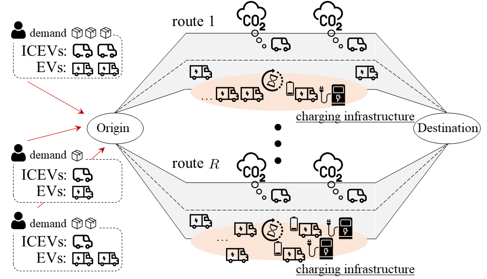
We model strategic routing decisions by multiple logistic operators (players). Each player’s fleet consists of a mix of EVs and traditional ICEVs. Players are required to deliver a predetermined amount of commodities (i.e. demand) from an origin node to a common destination node. The players share a common EV charging infrastructure (specialized for heavy duty vehicles [19]) that is deployed over a parallel route network; see Fig. 1. Every player decides the share of the demand to be delivered by the ICEVs and EVs as well as the route used by each vehicle in her fleet. The player’s cost is comprised of operational and environmental costs. For sake of simplicity, we model these costs as the cost of delayed delivery at the destination node and pollution cost, respectively. We also suppose that the congestion externality faced by the vehicle fleets due to presence of the regular traffic is negligible relative to the congestion faced by EVs at the charging stations. In particular, the EVs are supposed to require access to charging stations to complete their trip due to the limitations of current battery technology. Furthermore, the “public” nature of charging facilities implies that the delay incurred in waiting and charging at these locations must be accounted by the players in their routing decisions. Thus, in our model, congestion only impacts the cost of delayed delivery of EVs. Again, for simplicity, we consider that the ICEVs face no delays on any route. However, players incur a pollution cost in the form of fuel and environmental tax for each ICEV that is routed through the network. In contrast, the electricity supply at the charging stations is “net-zero” and hence the players do not incur pollution costs in routing EVs through the network. The simplifying assumptions in our model are primarily governed by our intent to focus on the trade-off that the players face by incurring low cost of delayed delivery (resp. high pollution cost) when they choose a larger proportion of ICEVs instead of relaying on EVs that face congestion at charging stations.
Let denote the set of players. The amount of freight demand that needs to be delivered by player is given by . Players share a network of parallel routes denoted by . For simplicity, we assume that all ICEVs face an identical pollution cost regardless of the route assigned to them. Moreover, without loss of generality, we consider that all EVs necessarily need to recharge en-route; otherwise delivering all demand by EVs using the route becomes the trivial optimal routing for the operator, who has no interaction among the other players. We also consider that charging stations are placed at each route since roads without charging infrastructure cannot be exploited by EVs. For player , we denote the total demand delivered by ICEVs by (note that we do not need to track the ICEVs in each route because of route-independent pollution cost in our model). Similarly, we denote the demand delivered by EVs of player through route by . Then the action of player is represented as
where the action set is given by
The flow profile on the set of players is denoted by and its feasible set is denoted by . Denote the aggregated flow of EVs over each route by
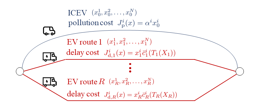
Due to the delay incurred by EVs while waiting at the charging stations, the total expected delivery duration for each route depends on the aggregate flow that is routed through it. We denote the delivery duration for route by with . On the other hand, the pollution cost linearly depends on the demand met by the ICEVs (although marginal cost of pollution can vary across players). Fig. 2 illustrates this setting.
The cost function of player , denoted by , is given by
| (1) |
where
with and that satisfies
| (2) |
with some . In (1), and represent the pollution cost and the delayed delivery cost associated with the route , respectively. Here represents the delayed delivery cost per unit time, where the condition (2) signifies that no cost is incurred for an early or on-time delivery. In addition, we make the following technical assumptions: For any and ,
-
•
is strictly increasing and convex for .
-
•
is strictly increasing and convex for .
-
•
and are twice continuously differentiable for and .
While is determined from the operational requirement, is composed of driving and charging duration. The driving duration is determined by the traffic congestion level, which can be estimated from data of GPS [20] or road sensors [21]. The charging duration is determined by the capacity of the charging facility [22].
In fact, we can simply express the delayed delivery cost as a function of the aggregated flow of each route by . Thus, we can write
Similarly, the aforementioned assumptions on and can be re-written as follows:
Assumption 1
For any and ,
-
•
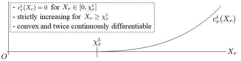
for any with some .
-
•
is strictly increasing for .
-
•
is convex and twice continuously differentiable for .
The form of is illustrated in Fig. 3. We refer to the interval as the cost-free interval of the route for player and the route where the aggregated flow is within the cost-free interval as a cost-free route given a flow profile. Its existence immediately suggests that players prioritize cost-free routes, and moreover, induces multiple equilibria as observed in Sec. III.
The model leads to an -player atomic routing game . We adopt Nash equilibrium (NE) as the solution concept:
Definition 1 (Nash Equilibrium)
A flow profile is said to be a NE of the game if
for any , where denotes the -th player’s cost function and denotes the flow profile of all players but .
We say that the NE of is essentially unique if the costs corresponding to all NE are equal.
Note that the existence of NE under Assumption 1 is straightforward from the well-known result: there exists a NE when every cost function is convex and every feasible region is compact and convex [23, Theorem 4.7.2].
Remark: We assume the total cost to be continuous with respect to the amount of the delivered commodities . In general, can be discontinuous in because the total amount of commodity depends on the batches transported by individual vehicles. Our model is obtained through smoothing on an implicit premise that the commodity amount delivered by a single vehicle is relatively small and the batch nature of transport can be ignored.
III EQUILIBRIUM ANALYSIS
III-A Existence of Multiple NE
Analysis of NE is a basis for quantifying inefficiency of selfish routing and designing effective economic mechanisms. When the NE is unique, the analysis becomes considerably simple. For example, price of anarchy (PoA) and price of stability, which are different measures of inefficiency, are identical in a game with a unique NE [10, Chap. 17]. However, the green routing game admits multiple NE in contrast to standard atomic splittable routing games over parallel networks [14, 16]. This subsection exhibits an example with multiple NE suggesting a condition for uniqueness of NE, which specifies tractable situations.
Example 1
Consider a 2-player game with two roads where for and . The cost function over the cost-free interval is given by a quadratic function for and . It can be shown that both
are NE. Moreover, the NE are not essentially unique. In fact, the costs of player 2 corresponding to the NE are given by
The NE are illustrated in Fig. 4, where denotes the marginal cost of the route for player .
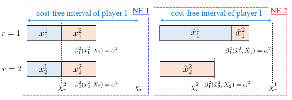
The second NE is obtained as follows: Since the aggregated flows are within the cost-free intervals for player 1 at the first NE, the equilibrium flow profile incurs no cost for player 1. Also, since the aggregated flow is strictly less than the threshold , moving a fraction of to the first route does not change the cost for player 1. Thus, is a best response to any routing of player 2 as long as . On the other hand, from the perspective of player 2, her reasonable action is changed by the lateral movement of player 1. The reasonable usage of EVs at each route is characterized by , which means that the marginal cost of each route is balanced with the marginal cost of usage of ICEVs given as . This results in the second NE. While the cost of player 1 is zero at both NE, the cost of player 2 varies, and hence those NE are not essentially unique.
This example suggests that the huge gap between the delayed delivery costs of the players causes the multiple NE. It is expected that, conversely the NE can be unique with cost functions identical with respect to players. The next subsection formally proves the uniqueness to specify tractable instances.
III-B Condition for Uniqueness of NE
The following assumption is made for the subsequent analysis.
Assumption 2
The delayed delivery cost functions are identical with respect to the players, i.e., for every .
In the following, we omit the superscript from . Practically, Assumption 2 holds when the operators provide the same service. A possible situation is that a customer at the destination orders goods from multiple logistic companies imposing the same delay penalty.
In fact, Assumption 2 guarantees uniqueness of NE. The following theorem holds.
To prove Theorem 1, we first introduce three structural results about the NE. Note that, because the constraints associated with satisfy linear independence constraint qualification, a flow profile is a NE if and only if it satisfies the Karush-Kuhn-Tucker (KKT) conditions [24, Chap. 5]:
| (3) |
with Lagrange multipliers for every .
First, we claim that if there are cost-free routes at some NE, then all routes need to be cost-free at any NE.
Lemma 1
Proof.
Note that Assumption 2 implies that for any . We remove the superscript from . Let be the NE such that for some . We first prove that this NE satisfies for any by contradiction. Assume that there exists such that . Then there exists such that . From the complementarity condition, . Thus . On the other hand, since , . Therefore . However, since and , we have , which is a contradiction.
Finally, from the claim above, we have for every . Thus, for every feasible flow profile , which satisfies , there exists such that . Therefore every NE satisfies the condition. ∎
Lemma 1 implies that if there exists a NE that causes free-cost intervals under Assumption 2 then the NE are essentially unique. Thus, in what follows we can focus on NE at which there are no free-cost intervals. In the remainder of this subsection, we denote two NE with the corresponding Lagrange multipliers by and . Also, the corresponding aggregated flows denoted by and satisfy
| (4) |
Under this condition, we basically follow the proof of [16, Theorem 2]. The following lemma holds.
Lemma 2
Proof.
We show the first claim. Assume and . If then from the complementarity condition, and hence . If then . Since is monotonically non-decreasing in , . Since from Lemma 1, . Hence is strictly increasing in . Thus . Next, assume and . If then which implies or . If then . As in the deduction above, we have . Finally, the second and fourth items can be proven in the same manner.
In terms of the second claim, if then from (3). Thus the complementarity condition leads to . The second item can be proven in the same manner. ∎
Based on the preparation, we can show that the aggregated flow profiles of two NE are identical. The following lemma holds.
Proof.
Define and . Assume . Letting , we have for any from the first claim of Lemma 2. Since for any . From the second claim of Lemma 2, for and Hence
| (5) |
On the other hand, from the first claim of Lemma 2,
| (6) |
However, from the definition of , . This is a contradiction and hence . Similarly, does never happen. Therefore, the claim holds. ∎
Now we can prove Theorem 1.
Theorem 1.
If there exists a NE such that for some , then every NE incurs no cost and hence the NE is essentially unique from Lemma 1. In the following, we assume that (4) holds. If for , then for any and from the first claim of Lemma 2 and Lemma 3. Consider the case where for some . From the first claim of Lemma 2 and Lemma 3, or for any . Assume that there exists such that . Then . From the second claim of Lemma 2, and thus . This is in contradiction. Thus, in any case, for any and . Then we have . Therefore, . ∎
IV EQUILIBRIUM COMPUTATION
This section proposes an algorithm to compute the NE. Note that, the game is not a potential game unlike non-atomic routing games. Hence the algorithm that allows players to iteratively play best responses, and is guaranteed to converge to a NE for potential games [25, Theorem 6.4.3], may not converge for our game.
Instead, we consider a gradient-based algorithm, referred to as simultaneous improving response dynamics (SIRD) proposed in [16], given by Algorithm 1. In SIRD, denotes the projection onto and denotes the gradient of with respect to . The constants and determine the step size and the stopping criterion, respectively. SIRD can be regarded as an extended version of the gradient projection method [26, Sec. 2.3], which was originally proposed for an optimization problem with a single decision maker. In SIRD, every player simultaneously carries out each iteration of the gradient projection method.
Our aim is to specify a condition with which SIRD converges to a NE. In [16], the convergence is proven under a mild condition for the case where there is no route corresponding to and the cost function is strictly increasing for the whole interval. They have identified a condition with which the gradients become strongly monotone [27, Definition 2.3.1], i.e., there exists such that
| (7) |
for any with . From the strong monotonicity each iteration in SIRD becomes a contraction, which leads to the convergence from the standard fixed point theorem.
However, in our model, the condition (7) does never hold because the aggregated gradient can be constant at two different points. Indeed, for any satisfying for any , we have and hence . By choosing such and , we have for . Thus it is clear that there does not exist that satisfies (7). Therefore, the iteration in SIRD is not a contraction and the standard fixed point theorem cannot be used in our case.
Instead of the logic above, we employ a variant of the fixed point theorem adapted to averaged maps. A vector-valued map is said to be nonexpansive if
Also, is said to be averaged if there exist and a nonexpansive map such that . It is known that iteration of an averaged map converges to a fixed point of the map [18, Theorem 2.1]. Furthermore, we need the notion of co-coercive [27, Definition 2.3.9] as an alternative to strong monotonicity: A map is said to be co-coercive if there exists such that
for any . In what follows we show that if is co-coercive then the iteration in SIRD is averaged, and hence it converges to a NE.
We start with showing that is co-coercive under the condition provided in [16]. The following lemma holds.
Lemma 4
Proof.
Let denote the Jacobian of given by . Note that if is positive semidefinite for any then there exists such that
which implies that is co-coercive [27, Prop. 2.9.25 (a)]. Thus it suffices to show that is positive semidefinite for the former claim.
We re-index to be block-diagonal by with Then we have
For , every component is zero. For ,
Denote the quadratic form by for a fixed . By omitting notation and for simplicity, we have
Let and .
If , we have
Thus the quadratic form can be decomposed as with and where and Note that
and From Weyl’s inequality [28, Theorem 4.3.1], we have
Thus if and , the latter of which is equivalent to (8), then is positive semidefinite.
On the other hand, if , then and hence . Then and hence the matrix is positive semidefinite for any and .
After all, if (8) holds, then is positive semidefinite. Because is block diagonal, we have Therefore, is also positive semidefinite.
We show the latter claim. Note that Now we have
because is co-coercive with modulus . Thus is nonexpansive. This implies that is averaged for . Finally, because the composition of a projection and an averaged map is also averaged [18, Proposition 2.1], the latter claim holds. ∎
Lemma 4 indicates that a NE can be computed using SIRD.
Theorem 2
V NUMERICAL EXAMPLE
V-A Simulation Parameters
We present a numerical example to discuss properties of the game based on the theoretical developments. Consider a two-player game with two routes, i.e., and . The demands are set by and . We consider the delivery duration in a linear form of with and . Let and . The delayed delivery cost function is set to a quadratic function given by for . Note that those functions satisfy Assumption 1. This choice leads to for .
V-B Effectiveness of SIRD
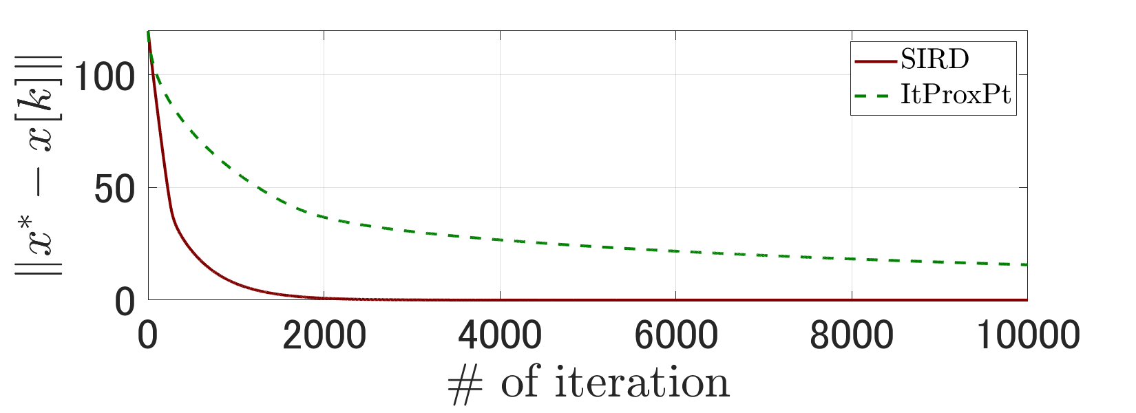
We first observe the effectiveness of the proposed algorithm with comparison to the distributed iterative proximal-point algorithm, referred to as ItProxPt, proposed in [15]. The ItProxPt algorithm is a gradient-based algorithm as well, and Line 5 in Algorithm 1 is replaced with where the time-varying parameter is set to satisfy the Robbins-Monro condition [29, Chapter 2] and is a constant. Specifically, we set and . Let , under which both players have the same delayed delivery cost function. Fig. 5 draws the convergence rate of the algorithms for an instance with , where the solid line corresponds to SIRD while the broken line corresponds to ItProxPt. The horizontal and vertical lines describe the number of iteration and the norm of the error from the NE, respectively. First, it is observed that SIRD successfully finds the NE. Second, it is also observed that, SIRD converges to the NE very quickly compared with ItProxPt. This arises from the property that the step size can be fixed in SIRD while it is time-varying and converges to zero in ItProxPt.
V-C Inefficiency of NE
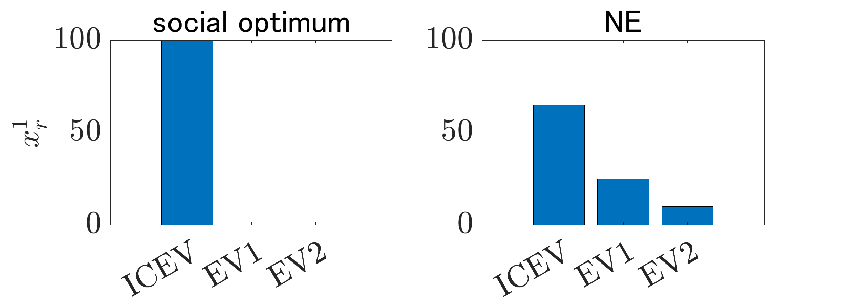
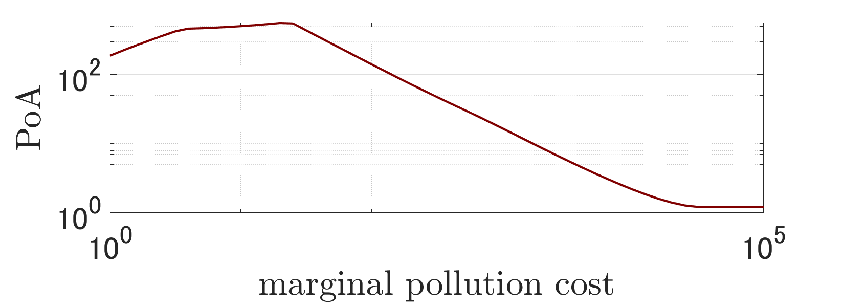
We adopt the summation of the players’ costs as the objective function. Also, inefficiency of NE is measured by PoA, namely, the ratio between the worst social cost of a NE and that of an optimal outcome [10, Chap. 17]. Fig. 6a depicts the socially optimal profile and the unique NE of the instance considered in the previous subsection. The PoA is 187.6. As suggested by the extremely large PoA, the social optimum and the NE are considerably different. It can be observed that player 1 fully uses ICEVs at the social optimum, while she assigns moderate shares to EVs at the NE. A possible approach to reduce inefficiency is to increase the marginal pollution cost. Let with a varying parameter . Fig. 7 draws the PoA where the horizontal line is . It is observed that the PoA when is about 1.2. The social optimum and the NE with high marginal pollution cost are depicted in Fig. 6b.

V-D Multiple NE Case
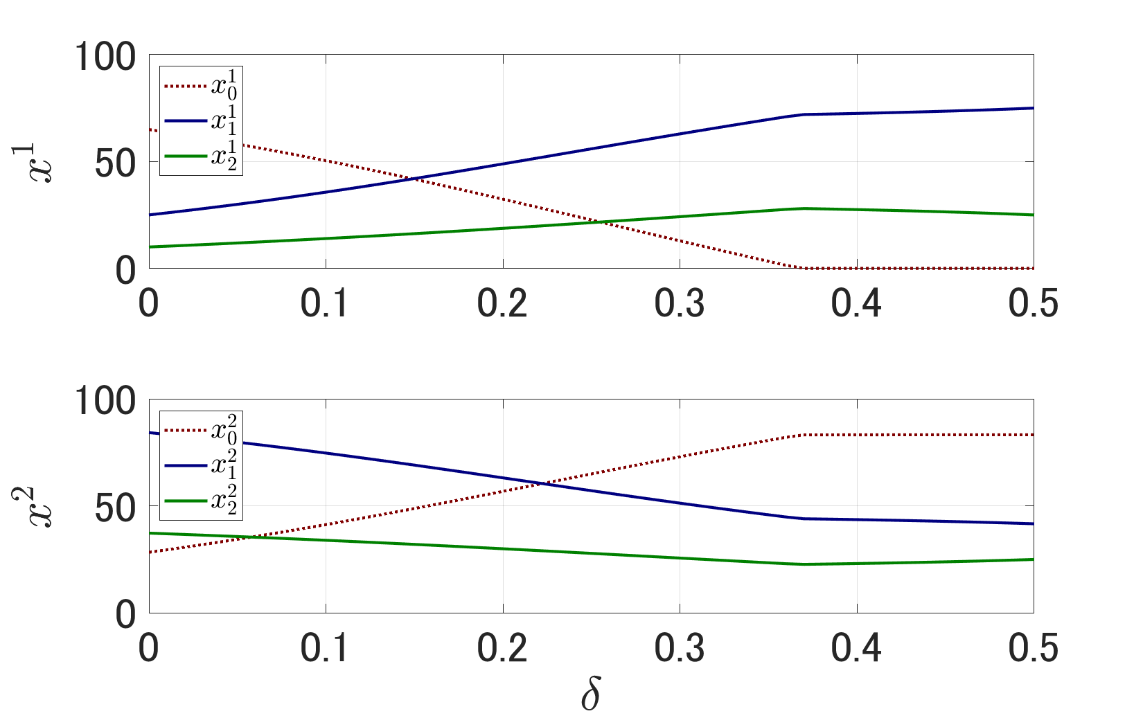
Next, we investigate a condition for existence of multiple NE. Introduce a parameter that prolongs the required delivery time of player 1 by . In fact, as increases, the gap between the cost functions of the players increases, which leads to existence of multiple NE as expected in Sec. III-A. It can be confirmed that the NE is unique when . Fig. 8 depicts the equilibrium flow profile with varying . When is large, player 1 uses only EVs due to less strict requirement. When the gap between the cost functions are such huge that multiple NE arises.
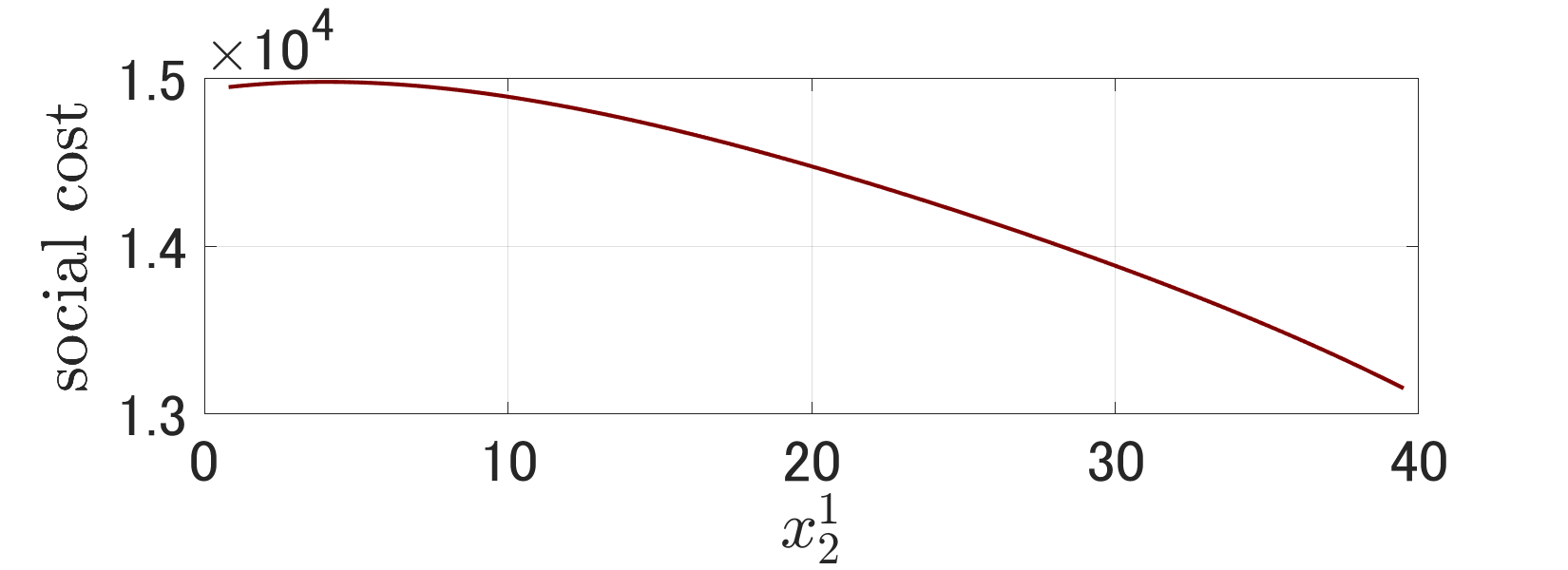
Finally, we observe inefficiency of multiple NE. Let and then there exist multiple NE. It can be confirmed that can be a NE with the best response of player 2 for . Fig. 9 depicts the social cost corresponding to each NE. It is observed that the social cost is minimized when is maximized. Note that and , and hence the route 2 is the most time-consuming route. This result suggests that it is socially desirable that players whose time requirement is less strict than the others put all demand to the most time-consuming routes.
VI CONCLUSION
The paper has formulated a green routing game, where the cost is composed of pollution and delayed delivery with interaction caused by congestible nature at public charging stations. In contrast to standard routing games, the game admits multiple NE. It has been shown that the NE is unique when the delayed delivery cost functions are identical with respect to players. Moreover, a distributed algorithm has been proposed. Numerical results have revealed several properties of the green routing game. In particular, it is suggested that high marginal pollution cost can reduce inefficiency of selfish routing. The obtained results provide insights for mechanism design of internalizing congestion and environment externality. Future work includes theoretical analysis of PoA.
References
- [1] European Environment Agency, “National emissions reported to the UNFCCC and to the EU greenhouse gas monitoring mechanism,” 2021, [Online]. Available: https://www.eea.europa.eu/data-and-maps/data/national-emissions-reported-to-the-unfccc-and-to-the-eu-greenhouse-gas-monitoring-mechanism-17.
- [2] European Commission, “Stepping up Europe’s 2030 climate ambition,” 2020, [Online]. Available: https://eur-lex.europa.eu/legal-content/EN/TXT/?uri=CELEX:52020DC0562.
- [3] J. Y. Yong, V. K. Ramachandaramurthy, K. M. Tan, and N. Mithulananthan, “A review on the state-of-the-art technologies of electric vehicle, its impacts and prospects,” Renewable and Sustainable Energy Reviews, vol. 49, pp. 365–385, 2015.
- [4] T. Bektaş and G. Laporte, “The pollution-routing problem,” Transportation Research Part B: Methodological, vol. 45, no. 8, pp. 1232–1250, 2011.
- [5] M. Schneider, A. Stenger, and D. Goeke, “The electric vehicle-routing problem with time windows and recharging stations,” Transportation Science, vol. 48, no. 4, pp. 500–520, 2014.
- [6] D. Goeke and M. Schneider, “Routing a mixed fleet of electric and conventional vehicles,” European Journal of Operational Research, vol. 245, no. 1, pp. 81–99, 2015.
- [7] Ç. Koç and I. Karaoglan, “The green vehicle routing problem: A heuristic based exact solution approach,” Applied Soft Computing, vol. 39, pp. 154–164, 2016.
- [8] Z.-J. M. Shen, B. Feng, C. Mao, and L. Ran, “Optimization models for electric vehicle service operations: A literature review,” Transportation Research Part B: Methodological, vol. 128, pp. 462–477, 2019.
- [9] M. Asghari and S. Al-e-hashem, “Green vehicle routing problem: A state-of-the-art review,” International Journal of Production Economics, vol. 231, 2021.
- [10] N. Nisan, T. Roughgarden, Éva Tardos, and V. Vazirani, Eds., Algorithmic Game Theory. Cambridge University Press, 2007.
- [11] W. Krichene, J. D. Reilly, S. Amin, and A. M. Bayen, “Stackelberg routing on parallel networks with horizontal queues,” IEEE Trans. Autom. Control, vol. 59, no. 3, pp. 714–727, 2014.
- [12] D. A. Lazar, S. Coogan, and R. Pedarsani, “Routing for traffic networks with mixed autonomy,” IEEE Trans. Autom. Control, vol. 66, no. 6, pp. 2664–2676, 2021.
- [13] M. Wu, S. Amin, and A. E. Ozdaglar, “Value of information in Bayesian routing games,” Operations Research, vol. 69, no. 1, pp. 148–163, 2021.
- [14] A. Orda, R. Rom, and N. Shimkin, “Competitive routing in multiuser communication networks,” IEEE/ACM Transactions on Networking, vol. 1, no. 5, pp. 510–521, 1993.
- [15] H. Chen, Y. Li, R. H. Louie, and B. Vucetic, “Autonomous demand side management based on energy consumption scheduling and instantaneous load billing: An aggregative game approach,” IEEE trans. Smart Grid, vol. 5, no. 4, pp. 1744–1754, 2014.
- [16] P. Jacquot, O. Beaude, S. Gaubert, and N. Oudjane, “Analysis and implementation of an hourly billing mechanism for demand response management,” IEEE Trans. Smart Grid, vol. 10, no. 4, pp. 4265–4278, 2018.
- [17] P. Jacquot and C. Wan, “Routing game on parallel networks: The convergence of atomic to nonatomic,” in IEEE Conference on Decision and Control (CDC), 2018, pp. 6951–6956.
- [18] C. Byrne, “A unified treatment of some iterative algorithms in signal processing and image reconstruction,” Inverse Problems, vol. 20, pp. 103–120, 2003.
- [19] B. Al-Hanahi, I. Ahmad, D. Habibi, and M. A. Masoum, “Charging infrastructure for commercial electric vehicles: Challenges and future works,” IEEE Access, vol. 9, pp. 121 476–121 492, 2021.
- [20] D. B. Work, S. Blandin, O.-P. Tossavainen, B. Piccoli, and A. M. Bayen, “A traffic model for velocity data assimilation,” Applied Mathematics Research eXpress, vol. 2010, no. 1, pp. 1–35, 2010.
- [21] N. G. Polson and V. O. Sokolov, “Deep learning for short-term traffic flow prediction,” Transportation Research Part C: Emerging Technologies, vol. 79, pp. 1–17, 2017.
- [22] A. Tomaszewska, Z. Chu, X. Feng, S. O’Kane, X. Liu, J. Chen, C. Ji, E. Endler, R. Li, L. Liu et al., “Lithium-ion battery fast charging: A review,” ETransportation, vol. 1, 2019.
- [23] R. Laraki, J. Renault, and S. Sorin, Mathematical Foundations of Game Theory, ser. Universitext. Springer, 2019.
- [24] S. Boyd and L. Vandenberghe, Convex Optimization. Cambridge University Press, 2004.
- [25] Y. Shoham and K. Leyton-Brown, Multiagent systems: Algorithmic, game-theoretic, and logical foundations. Cambridge University Press, 2008.
- [26] D. P. Bertsekas, Nonlinear Programming. Athena Scientific, 1998.
- [27] F. Facchinei and J.-S. Pang, Finite-Dimensional Variational Inequalities and Complementarity Problems. Springer, 2003.
- [28] R. A. Horn and C. R. Johnson, Matrix Analysis, 2nd ed. Cambridge University Press, 2012.
- [29] V. S. Borkar, Stochastic Approximation: A Dynamical Systems Viewpoint. Springer, 2009.