Measuring magic on a quantum processor

Abstract

Magic states are the resource that allows quantum computers to attain an advantage over classical computers. This resource consists in the deviation from a property called stabilizerness which in turn implies that stabilizer circuits can be efficiently simulated on a classical computer. Without magic, no quantum computer can do anything that a classical computer cannot do. Given the importance of magic for quantum computation, it would be useful to have a method for measuring the amount of magic in a quantum state. In this work, we propose and experimentally demonstrate a protocol for measuring magic based on randomized measurements. Our experiments are carried out on two IBM Quantum Falcon processors. This protocol can provide a characterization of the effectiveness of a quantum hardware in producing states that cannot be effectively simulated on a classical computer. We show how from these measurements one can construct realistic noise models affecting the hardware.

Introduction

In the era of Noisy Intermediate Scale Quantum Computers (NISQs)[1] it is of paramount importance to be able to characterize the proposed quantum hardware in order to check how good these machines are in performing quantum computation with the purpose of attaining an advantage over classical computers. This paper shows how to perform accurate and robust measurements of the stabilizer Rényi entropy, which in turn is known to quantify the resource known as ‘magic’[2] It is well known that the preparation of stabilizer states, the implementation of Clifford gates and measurements in the computational basis can be made fault tolerant[3, 4, 5, 6, 7, 8, 9]. However, computers based on the Clifford resources can be efficiently simulated on classical computers[10, 11, 12, 13], similarly to what happens for matchgate circuits(MGCs). This means that the power of quantum advance requires resources beyond the Clifford group, like the Phase $\pi/8$ gate (T gate) or the Toffoli gate and non-Gaussian states for the MCGs[14, 15]. The precious resource that makes quantum computers special is colloquially dubbed as ‘magic’ and a resource theory of magic has been developed in recent years[3, 4, 16, 17, 18, 19, 20, 21, 2, 22, 23, 24, 25, 26, 27].

It is a striking fact that these resources are difficult to implement[3, 5, 28, 29, 30, 31, 32, 33]. The very reason why these resources are powerful makes them fragile. Moreover, the amount of these resources that needs to be used in a computation must be calibrated accurately: just like entanglement[34], too much magic is not useful for quantum computation (see Supplementary Note $1$), see also[21]. Moreover, decoherence is not magic preserving, and it can both increase or decrease the amount of magic in a system, as we will show in the experiments. To the extent that decoherence is spoiling quantum computation, then one needs the amount of magic created and manipulated throughout the computation to be accurate: in this paper, we prove that an excess amount of unwanted magic makes the task of distinguishing the state $\psi$ from a random state an exponentially difficult task, see Supplementary Note $1$ for the proof. Moreover, since inaccurate Clifford gates can produce magic, the presence of excess magic is in fact a signal of noise. We exploit this fact to show that the measurement of magic can be used to quantify and characterize the noise in the quantum circuit. It is thus important to be able to quantify this resource and measure it to characterize the fitness of real quantum hardware. Unfortunately - until recently - proposed measures of magic[4, 17, 35, 22] have been based on extremization procedures and no experimental measurement scheme has been proposed.

In this work, we propose and experimentally demonstrate a protocol based on randomized measurements[36, 37, 38, 39, 40, 41, 42, 43, 44, 45, 46, 47, 48, 49] to measure magic in a quantum system with $n$ qubits and to characterize quantum hardware. We adopt the magic measure called stabilizer $2$-Rényi entropy defined as[2]

$$M_{2}(\mid\!\psi\rangle):=-\log_{2}W(\psi)-S_{2}(\psi)-\log d$$ (1)

where $W(\psi):=\operatorname{tr}(Q\psi^{\otimes 4})$, $Q:={d^{-2}}\sum_{P}P^{\otimes 4}$ and $d=2^{n}$, where the sum is taken over all multi-qubit strings of Pauli operators, applied to four copies of the state, and $S_{2}(\psi)=-\log_{2}\operatorname{tr}{\psi^{2}}$ is the $2$-Rényi entropy. In order to measure $M_{2}$ we propose an improved protocol compared to the one presented in Ref. [2] as it only involves randomized one-qubit measurements instead of global multi-qubit measurements, with obvious advantages in terms of errors and quantum control.

As $M_{2}$ depends on the state $\psi$, a direct evaluation of $M_{2}$ would be possible by knowing all the expectation values $\operatorname{tr}(P\psi)$ of multi-qubit Pauli strings in the state $\psi$. This, of course, is equivalent to tomography and it is very expensive as it involves the evaluation of $d^{2}$ expectation values for a total cost in resources scaling as $\mathcal{O}(d^{3})$. Here, we employ a protocol based on randomized measurements which does not rely on tomographic techniques. Remarkably, randomized measurement protocols are highly favorable compared to state tomography[38, 39, 41, 43]. As we shall see, we will employ a number of resources scaling as $\mathcal{O}(\epsilon^{-2}d^{2})$ for an estimate with error $\epsilon$.

Results

The protocol

The protocol consists in first drawing a string of random one-qubit Clifford operations, namely $C=\bigotimes_{i=1}^{n}c_{i}$ and applying it to four copies of the state of interest. The protocol extracts correlations between these copies. Indeed, the quantity of interest in the first term of Eq. (1) can then be computed as

$$-\log_{2}\operatorname{tr}(Q\psi^{\otimes 4})=-\log_{2}\sum_{\vec{\mathbf{s}}}(-2)^{-\|\vec{\mathbf{s}}\|}\mathbb{E}_{C}P(\mathbf{s}_{1}\!\mid\!C)P(\mathbf{s}_{2}\!\mid\!C)P(\mathbf{s}_{3}\!\mid\!C)P(\mathbf{s}_{4}\!\mid\!C)$$ (2)

The formula above features the expectation value over the randomized measurements of the Clifford operator $C$ on states of the computational basis $\mathbf{s}_{a}$ and the Hamming weight $\|\vec{\mathbf{s}}\|$ of the string $\mathbf{s}_{1}\oplus\mathbf{s}_{2}\oplus\mathbf{s}_{3}\oplus\mathbf{s}_{4}$. The quantity $P(\mathbf{s}_{a}\!\mid\!C)=\operatorname{tr}({C\psi C^{\dagger}}\mathbf{s}_{a})$ represents the probability of finding the computational basis state $\mathbf{s}_{a}$ when measuring the state $C\psi C^{\dagger}$. The second term in Eq. (1) is the usual $2$-Rényi entropy and can be measured by randomized measurements using the techniques of Ref. [41]. An important feature of our protocol is the fact that it only needs randomized operations over the Clifford group instead of the full unitary group as in Ref. [38]. In fact, by collecting the occupation probabilities $P(C\psi C^{\dagger}\!\mid\!\mathbf{s}_{a})$ one can estimate both $W(\psi)$ and the purity $P(\psi)$ together thanks to the fact that the Clifford group forms a $2$-design. See Methods. The operational meaning of the protocol is the following: randomized measurement protocols are usually conducted on a (Haar) random basis. Here we select a (local) stabilizer basis. Clifford rotations constitute the free resources for magic state resource theory. General unitaries would result in a change in quantum magic. Clifford orbits of a given quantum state instead are filled out by iso-magic states. A Clifford randomized measurement protocol measures the magic of the entire Clifford orbit, rather than of a single quantum state.

The experiments have been conducted on two IBM Quantum Falcon processors: a $5$ qubit system, ibmq$\_$quito and a $7$ qubit system ibmq$\_$casablanca[50].

The experiment can be schematized as follows (see Fig. 1). Starting with a $n$-qubit state initialized in the $\mid\!0\rangle^{\otimes n}$ state, we pass it through a unitary quantum circuit $U$ resulting in the state preparation $\mid\!\!\psi\rangle$. We want to characterize the fitness of such a circuit in providing a state with the promised magic. At this point, one extracts $n$ one-qubit Clifford operations $c_{i}$, applies them to the state $\!\mid\!\psi\rangle$, and measures the state in the computational basis.

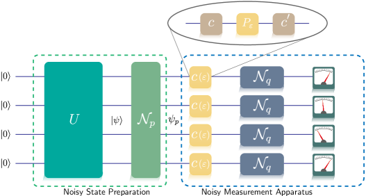
Figure 1: Schematic of the implementation of the experiment for measuring magic on a quantum processor. From left to right: Initialization of the system in the state $\!\mid\!\!0\rangle^{\otimes n}$; preparation of the target state $\mid\!\psi\rangle$ by a unitary quantum circuit $U_{t}$ containing a number $t$ of non-Clifford gates; intervention of the noise $\mathcal{N}_{p}$ affecting the system effectively prepares the (mixed) state $\psi_{p}$; measurement. The measurement apparatus is composed of $n$ local Clifford operators $C=\bigotimes_{i=1}^{n}c_{i}$ randomly sampled from the single qubit Clifford group $c_{i}\in\mathcal{C}_{1}$, followed by $n$ measurements in the computational basis $\{\mid\!\mathbf{s}\rangle\}$ which are performed to estimate the occupation probabilities $P(C\psi C^{{\dagger}}\!\mid\!\mathbf{s})$. The gate imperfection in the application of the Clifford operators is denoted by $c(\epsilon)$.

At this point, we want to analyze the scaling of the cost of necessary resources, both analytically and numerically. The experiment is repeated $N_{M}$ times for every string $C=\bigotimes_{i=1}^{n}c_{i}$ in order to collect statistics to compute the occupation probabilities $P(C\psi C^{\dagger}\!\mid\!\mathbf{s}_{a})$. Then, in order to compute the expectation value over the whole Clifford group $\mathbb{E}_{C}$, one samples the Clifford group with $N_{U}$ elements. In order to sample the Clifford group properly and to build sufficient statistics we simulate numerically the total number of measurements needed for $M_{2}$, i.e. $N_{TOT}=N_{M}\times N_{U}$. By evaluating the variance of the estimator for $W$, through the use of standard statistical analysis (Bernstein inequality), one can bound the probability of making an error $\epsilon$ as a function of the total resources $N_{U}\times N_{M}$ employed. In Methods, we prove that by employing a total number of resources $\mathcal{O}(\epsilon^{-2}d^{2})$ the randomized measurement protocol is able to estimate the purity within an error $\leq\epsilon$ and the stabilizer purity within an error $\epsilon d^{-1}$. These theoretical bounds can be optimized by numerical analysis. The optimal number of unitaries $N_{U}$ and of measurements $N_{M}$ is found by numerical simulations imposing that the relative error on the theoretical value of stabilizer purity to be below $12\%$ and an average value of the purity greater than $0.88$, thus imposing a relative error of $12\%$ on the purity as well. An important remark is that both $N_{U}$ and $N_{M}$ depend on the state $\psi$. Remarkably, low-magic states (like the states in the computational basis - which have exactly zero magic) require a higher $N_{U}\times N_{M}$ compared to states with high magic, see Supplementary Table I in Supplementary Note $4$.

In order to characterize the fitness of a quantum processor in producing resources beyond stabilizer states, we adopt the model of a $t$-doped Clifford circuit[51, 52, 53]. This circuit consists of a block of Clifford gates in which $t$ non-Clifford gates are injected. The non-Clifford gates we inject are $P_{\vartheta}=\mid\!\!0\rangle\langle 0\!\!\mid+e^{i\vartheta}\mid\!\!1\rangle\langle 1\!\!\mid$ gates: these constitute the resources that are injecting magic in the system, while the Clifford circuits are free resources. For $\vartheta=\pi/2$ one obtains the phase flip gate that still belongs to the Clifford group and thus is a free resource. The value $\vartheta=\pi/4$ instead, the so-called $T$ gate, yields the maximal amount of magic achievable for a $P_{\vartheta}$ gate. The $T$-gates will be called the “magic seeds” of the quantum circuit. These circuits are efficient in entangling so the output state of the circuit is in general not a trivial product state but a state that is both entangled and possesses magic.

Measuring magic

We start with the characterization of the quantum processor on single-qubit states, and thus without entanglement. The single-qubit magic states are obtained by applying $P_{\vartheta}$ on the states $\mid\!\!+\rangle=\frac{1}{\sqrt{2}}(\mid\!\!\!\!\,0\rangle+\!\mid\!\!\!\!\,1\rangle)$ obtaining $\mid\!\!P_{\vartheta}\rangle\equiv P_{\vartheta}\!\!\mid\!\!+\rangle=\frac{1}{\sqrt{2}}(\mid\!\!0\rangle+e^{i\vartheta}\!\mid\!\!1\rangle)$ whose stabilizer $2$-Rényi entropy reads $M_{2}(\mid\!\!P_{\vartheta}\rangle)=-\log_{2}\left(\frac{7+\cos(4\vartheta)}{8}\right)$, achieving its maximum for $M_{2}(\mid\!\!P_{\pi/4}\rangle)=1-\log_{2}3/2$ and its minimum for $M_{2}(\mid\!\!P_{\pi/2}\rangle)=0$.

The results of the experiment on the ibmq$\_$quito are shown in Fig. 2. As we can see, the experimental data are in very good accordance with the theoretical prediction for the target state, showing the fitness of ibmq$\_$quito in preparing single-qubit magic states. Decoherence effects are also very low, as we can see from the purity, see Fig. 2.

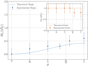
Figure 2: Stabilizer $2$-Rényi entropy for $\mid\!\!P_{\vartheta}\rangle$. Plot of the magic of the single qubit $\mid\!\!P_{\vartheta}\rangle$-states, for $\theta=0,\frac{\pi}{16},\frac{\pi}{8},\frac{\pi}{6},\frac{\pi}{5},\frac{\pi}{4}$. The data displayed (blue dots) are obtained from the quantum processor ibmq$\_$quito. The blue dashed curve represents the theoretical value of the magic for $\mid\!\!P_{\vartheta}\rangle$-states, i.e. $M_{2}(\mid\!\!P_{\vartheta}\rangle)=3-\log_{2}\left(7+\cos(4\vartheta)\right)$. Additionally, a plot of the purity for these states is displayed in the upper right corner: as the data show, the purity is $1$ within the experimental errors, showing that the decoherence affecting the system is negligible for $n=1$ and also the experimental values of magic are in perfect agreement with the theoretical ones. See Supplementary Table II in the Supplementary Note $4$ for the data.

We now proceed to the more difficult task of characterizing a quantum processor capable of preparing entangled states. Starting from the computational basis state $\!\mid\!\!\!0\rangle^{\otimes n}$, i.e. the input state of the quantum processor, we first apply a layer of Hadamard $H$-gates to obtain $\!\mid\!\!\!+\rangle^{\otimes n}=H^{\otimes n}\!\mid\!\!0\rangle^{\otimes n}$. Then, we apply $T$-gates on $n_{1}$ qubits, with $n_{1}=0,\dots,n$. The $T$-gates inject magic into the system. For $n_{1}=n$, the state obtained is the maximal magic product state achievable. If one wants to pump more magic into the system, one needs to create some entanglement between the qubits. To do so, we apply a layer of CX-gates, i.e. Clifford entangling $2$-qubit gates defined as $CX_{i,j}=I_{i}\otimes(I_{j}+X_{j})+Z_{i}\otimes(I_{j}-X_{j})$ and nested in the following way: $CX_{n-1,n}CX_{n-2,n-1}\cdots CX_{1,2}$. Then we can inject some more magic in the system by applying another layer of $n_{2}$ $T$-gates with $n_{2}=1,\dots,n-1$ followed by another layer of $CX$: $CX_{1,2}\cdots CX_{n-2,n-1}CX_{n,n-1}$. For the pictorial representation of the previously described architecture see Fig. 3. At the end of the state preparation, the magic seeds in the circuit are $t=n_{1}+n_{2}$ and the state prepared is the $\mid\!\!\Gamma^{(n)}_{(n_{1},n_{2})}\rangle$-state, where $1\leq t\leq 2n-1$. In the following, we fill in $T$-gates starting from $(0,1)$, then $(n_{1},1)$ with $(n_{1},=1,\ldots,n;n_{2}=1)$, and finally $(n,n_{2})$, with $n_{2}=2,\ldots,n-1$. With this prescription, the label $t$ uniquely describes the circuit. For example, $t=4$ on a system with $n=6$ qubits means three $T$-gates on the first layer and one $T$-gate on the second layer, see Fig. 3. The optimal number of $N_{U},N_{M}$ for a system with $n=3,4,5$ qubits can be found in Supplementary Table I in Supplementary Note $4$ and Fig. 7 in Methods.

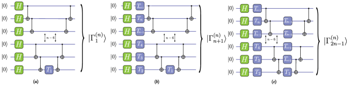
Figure 3: Preparation of $\mid\!\!\Gamma_{t}^{(n)}\rangle$ states. The magic seeds ($T$-gates) are placed either on the first layer (immediately after the Hadamard gates $H$), or in the second layer (immediately after the first layer of $C-NOT$ gates). We start with a $T$-gate in the second layer, then start filling up the first layer. Upon completion of the first layer, we start filling up the second layer again. The figure shows: $\mathbf{(a)}$ $\mid\!\!\Gamma_{1}^{(n)}\rangle$, $\mathbf{(b)}$ $\mid\!\!\Gamma_{n+1}^{(n)}\rangle$ and $\mathbf{(c)}$ $\mid\!\!\Gamma_{2n-1}^{(n)}\rangle$ which is the final doped Clifford circuit which we consider in this paper.

In a system with $n$ qubits we can prepare the states $\mid\!\!\Gamma^{(n)}_{t}\rangle$ with $t=1,\ldots,2n-1$. The results of the experiment for $n=3,4,5$ are shown in Figs. 4, 5,6, respectively. We can see that, for larger values of $n$, the purity of the prepared state is compromised, due to decoherence. The measured experimental values of magic shoot off the theoretical prediction, especially for low magic states. Somewhat counterintuitively, the experimental value of magic is higher than the theoretical one. As we mentioned above, spurious injection (or subtraction) of magic can happen for two reasons. Inaccurate implementation of the Clifford gates - and thus turning them into non-free resources - or noise affecting them, or decoherence. That is, our experimental characterization of how magic is created in a quantum circuit tests not only the quantity of magic, but the accuracy with which the desired magic is created. The fact that the circuit must not only create magic, but must do it so with a certain accuracy, allows us to use the experimental data obtained from our protocol to characterize the noise affecting the system. A first insight comes from the realization, see Figs. 4, 5, 6 that the noise is affecting more the preparation of low-magic states than that of high-magic states, mostly because of imperfection in the implementation of the resource-free Clifford gates like the CX gate. Let us see how we can characterize the noise affecting the system. A very general error model for the target state $\psi$ is through a quantum channel $\mathcal{E}(\psi):=\sum_{i}q_{i}P_{i}\psi P_{i}$. Random states are a good model for high-magic states[2] and thus, to understand why the noise affecting the system does not disturb the magic injected in high-magic states, we compute the average difference in magic between a random state $\psi$ and the noisy state $\mathcal{E}(\psi)$ as: $\langle\delta M\rangle_{Haar}:=\langle\mid\!M(\mathcal{E}(\psi))-M(\psi)\!\mid\rangle_{Haar}$. Calculation shows (see Supplementary Note 2) that $\langle\delta M\rangle_{Haar}=\mathcal{O}(S_{2}(\mathbf{q}))$. In other words, at high levels of magic, this quantity is robust under the noise model provided that the distribution $\mathbf{q}=\{q_{i}\}$ is low in entropy $S_{2}(\mathbf{q})$.

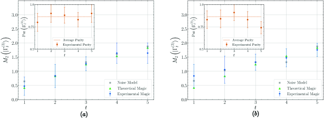
Figure 4: Stabilizer $2$-Rényi entropy for $n=3$. Plot of the stabilizer $2$-Rényi entropy for $\mathbf{(a)}$ ibmq$\_$quito and $\mathbf{(b)}$ ibmq$\_$casablanca. Both figures contain the experimental values (blue dots), the theoretical values (green triangles) of the magic for the desired pure state, and the noise model values (grey squares) of the magic for the mixed state prepared on the quantum processor. The values of the magic of the $\mid\!\!\Gamma^{(3)}_{t}\rangle$-states for $t=1,\dots,5$ are plotted as functions of the number of $T$-gates $t$ in the doped random Clifford circuits (see Supplementary Tables III and IV in the Supplementary Note $4$ for the data). See Fig. 3 for the preparation of such states. Both figures contain in the upper left corner the purity (orange dots) of the output state prepared on the quantum processor and its average value (dashed line). Here the number of resources $N_{TOT}\equiv N_{U}\times N_{M}$ depends on the number of $T$-gates $t$ thrown in the circuits as $N_{TOT}=2^{A_{3}+B_{3}(5-t)}$, where $A_{3}=10.6\pm 0.3$, $B_{3}=0.56\pm 0.08$, see Supplementary Table I in the Supplementary Note $4$ and Fig. 7 in Methods. Note that the experimentally observed magic can be – and typically is – higher than the theoretically predicted magic. This is because imperfectly performed Clifford gates are no longer exactly Clifford and can inject uncontrolled/unwanted magic into the system. This effect is enhanced for more qubits and deeper circuits.

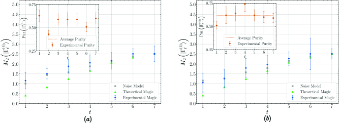
Figure 5: Stabilizer $2$-Rényi entropy for $n=4$. Plot of the stabilizer $2$-Rényi entropy for $\mathbf{(a)}$ ibmq$\_$quito and $\mathbf{(b)}$ ibmq$\_$casablanca. Both figures contain the experimental values (blue dots), the theoretical values (green triangles) of the magic for the desired pure state, and the noise model values (grey squares) of the magic for the mixed state prepared on the quantum processor. The values of the magic of the $\mid\!\!\Gamma^{(4)}_{t}\rangle$-states for $t=1,\dots,7$ are plotted as functions of the number of $T$-gates $t$ in the doped random Clifford circuits, (see Supplementary Tables III and IV in the Supplementary Note $4$ for the data). See Fig. 3 for the preparation of such states. Both figures contain in the upper left corner the purity (orange dots) of the output state prepared on the quantum processor and its average value (dashed line). Here the number of resources $N_{TOT}\equiv N_{U}\times N_{M}$ depends on the number of $T$-gates $t$ thrown in the circuits as $N_{TOT}=2^{A_{4}+B_{4}(7-t)}$, where $A_{4}=11.3\pm 0.3$, $B_{4}=0.49\pm 0.05$, see Supplementary Table I in Supplementary Note $4$ and Fig. 7 in Methods. Note that the experimentally observed magic can be – and typically is – higher than the theoretically predicted magic. See the caption of Fig. 4 for an explanation.

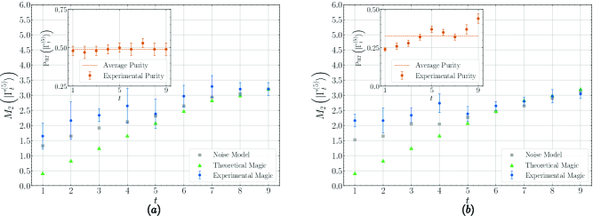
Figure 6: Stabilizer $2$-Rényi entropy for $n=5$. Plot of the stabilizer $2$-Rényi for $\mathbf{(a)}$ ibmq$\_$quito and $\mathbf{(b)}$ ibmq$\_$casablanca. Both figures contain the experimental values (blue dots), the theoretical values (green triangles) of the magic for the pure state one would have liked to obtain, and the noise model values (grey squares) of the magic for the mixed state prepared on the quantum processor. The values of the magic of the $\mid\!\!\Gamma^{(5)}_{t}\rangle$-states for $t=1,\dots,9$ are plotted as functions of the number of $T$-gates $t$ in the doped random Clifford circuits,(see Supplementary Tables III and IV in the Supplementary Note $4$ for the data). See Fig. 3 for the preparation of such states. Both figures contain in the upper left corner the purity (orange dots) of the output state prepared on the quantum processor and its average value (dashed line). Here the number of resources $N_{TOT}\equiv N_{U}\times N_{M}$ depends on the number of $T$-gates $t$ thrown in the circuits as $N_{TOT}=2^{A_{5}+B_{5}(9-t)}$, where $A_{5}=13.7\pm 0.1$, $B_{5}=0.047\pm 0.002$, see Supplementary Table I in the Supplementary Note and Fig. 7 in Methods. Note that the experimentally observed magic can be – and typically is – higher than the theoretically predicted magic. See the caption of Fig. 4 for an explanation.

Guided by this result, we model the noise in two factors (i) noise in state preparation due to decoherence and (ii) imperfection in the realization of the $c_{i}$ gates in the randomized measurement. This latter error is unitary. We then tune the factors quantifying the noise in our model to match the difference between the experimentally measured and the theoretically predicted amounts of magic.

The ansatz for the (non-unitary) quantum channel $\mathcal{N}_{p}$ affecting the state preparation is

$$\psi_{p}\equiv\mathcal{N}_{p}(\mid\!\!\psi\rangle\langle\psi\!\!\mid):=p\mid\!\!\psi\rangle\langle\psi\!\!\mid+\frac{(1-p)}{n}\sum_{i=1}^{n}Z_{i}\mid\!\!\psi\rangle\langle\psi\!\!\mid Z_{i}$$ (3)

where $Z_{i}$ is a phase flip error on the $i$-th qubit happening with probability $(1-p)/n$. This channel is not the simple phase-flip channel as the probability $p$ in principle depends on the target state $\mid\!\psi\rangle$. The imperfection in the gates $c_{i}$ is modeled by the unitary phase displacement $c_{i}\rightarrow c_{i}^{\varepsilon}\equiv c_{i}P_{\varepsilon}c_{i}^{\prime}$, where use the $P_{\varepsilon}$-gate described above. The measured stabilizer purity will be denoted by $W_{exp}(\mid\!\psi\rangle)$.

Our ansatz on how the noise affects the measurement results is then $W_{exp}(\mid\!\psi\rangle)\stackrel{{\scriptstyle\mathclap{\mbox{!}}}}{{=}}\operatorname{tr}(\psi_{p}^{\otimes 4}Q_{2}^{\varepsilon\otimes n})$ where $Q_{2}^{\varepsilon}$ represents the correction to the projector onto the single-qubit stabilizer code due to the gate imperfection error $\varepsilon$. The two free parameters $p$ and $\varepsilon$ can be determined experimentally, see Supplementary Note $2$.

Several points are in order here. First, notice that the purity $\operatorname{tr}{\psi_{p}^{2}}$ is protected against gate imperfection errors, so it can be measured independently. Second, one can measure the $\varepsilon$ error directly by measuring the purity of the initial state $\mid\!\!0\rangle^{\otimes n}$, thus avoiding the decoherence effect altogether. The values of the stabilizer $2$-Rényi entropy given by the noise model are represented by the Grey squares in Figs.4, 5 and 6 which show that they provide a better approximation to the experimental data, an approximation which in fact improves as the number of T gates in the circuit increases. By measuring the stabilizer $2$-Rényi entropy, thus, we provide a characterization of the noise model and an estimate of its parameters $p,\varepsilon$.

Discussion

Magic is a quantity of central importance for quantum computation: no quantum advantage can be obtained without it. This paper showed how to measure the amount of magic produced by a quantum circuit in terms of stabilizer Rényi entropy, and evaluated experimentally how that amount of magic scales as a function of the number of T-gates in the circuit. A central result of our experimental demonstration is that it is not enough just to create magic: the circuit must create an “accurate amount” of magic. Imperfectly implemented Clifford gates inject or subtract uncontrolled/unwanted magic into the circuit: just as excess entanglement can hinder the ability of a quantum circuit to perform some desired task[34], uncontrolled excess magic can result in the degradation of the performance of a quantum computation. Generating the correct amount of stabilizer Rényi entropy is thus an important component of the certification process for quantum hardware. More generally, in a quantum device, e.g. a circuit based on superconducting qubits, there can be errors beyond decoherence, like gate implementation errors, or other unitary errors. Typically, these errors are investigated through gate fidelity while the loss of purity is a good figure of merit to quantify decoherence. However, not always gate fidelity is available as a tool. As we can see in Figs. 4, 6, an inaccurate level of magic compared to the theoretical one signals the presence of unitary errors: a measurement of magic can then be used as a further tool to evaluate the accuracy of an experimental setup.

Methods

Theoretical framework

In [2] we proved that a global randomized measurements protocol can be employed to measure the stabilizer $2$-Rényi entropy for multiqubit states.

Here, we make a decisive improvement by establishing a protocol that only requires local measurements. Local measurements are usually the best measurements in terms of quantum control an experimenter has access to. Let us recall the definition of stabilizer $2$-Rényi entropy: for $\psi$ a $n$-qubit quantum state, the stabilizer $2$-Rényi entropy of $\psi$ is defined as $M_{2}(\psi):=-\log_{2}W(\psi)-S_{2}(\psi)-\log d$, where $W(\psi):=\operatorname{tr}(Q{\psi}^{\otimes 4})$, $S_{2}(\psi)=\operatorname{tr}(T\psi^{\otimes 2})$ and the operator $T$ is the swap operator while $Q:={d^{-2}}\sum_{P}P^{\otimes 4}$. The local randomized measurements protocol we introduce here aims at measuring $W(\psi)$ and $P(\psi)$ by only using single qubit gates and then measuring the qubits in the computational basis. In this way, we reduce access to multi-qubit gates that are typically noisier and whose control is poorer. The logic behind any randomized measurement protocol is to reconstruct operators (e.g. the swap operator for the purity or higher order permutations for higher order purities, see [36, 38, 39, 40, 43, 54, 55]) from correlations between randomized measurements. The measurement is randomized by means of Clifford single qubit gates. It is fundamental to use Clifford gates as magic is invariant under these unitary operations. The ideal experimental protocol for measuring simultaneously $W(\psi)$ and $P(\psi)$ is (see Fig.1 for a pictorial schematization):

1. pick $N_{U}$ random local Clifford operators $C=\bigotimes_{i=1}^{n}c_{i}$ where $c_{i}\in\mathcal{C}_{1}$ are single qubit Clifford gates. For each $C$ do:

   1. obtain the desired state $\psi$ from the quantum circuit $U$,

   2. apply $C$ on the state $\psi_{C}\equiv C\psi C^{\dagger}$,

   3. measure in the computational basis,

   4. redo steps $(i)$, $(ii)$ and $(iii)$ $N_{M}$ times to estimate the occupation probabilities $Pr(\psi_{C}\!\mid\!s)\equiv\operatorname{tr}(\mid\!\!s\rangle\langle s\!\!\mid\psi_{C})$ for $s=1,\dots,2^{n}$,

2. Estimate the probabilities $\tilde{Pr}(\psi_{C}\!\mid\!s)$ by measuring the frequencies of obtaining the bit-string $s_{2}$ in the state $\psi_{C}$. The estimator $\tilde{Pr}(\psi_{C}\!\mid\!s)$ for such probability converges to the true probability $Pr(\psi_{C}\!\mid\!s)$ in the limit $N_{M}\rightarrow\infty$.

3. Obtain $P(\psi)$ and $W(\psi)$ can be computed from the ideal probabilities $Pr(\psi_{C}\!\mid\!s)$ by:

   $$P(\psi) = \frac{1}{24^{n}}\sum_{C\in\mathcal{C}_{1}^{\otimes n}}\sum_{s_{1},s_{2}=1}^{2^{n}}O_{2}(s_{1},s_{2})Pr(\psi_{C}\!\mid\!s_{1})Pr(\psi_{C}\!\mid\!s_{2})$$ (4)

   $$W(\psi)\! = \!\!\frac{1}{24^{n}}\!\!\!\sum_{C\in\mathcal{C}_{1}^{\otimes n}}\sum_{s_{1},\dots,s_{4}=1}^{2^{n}}\!\!\!O_{4}(s_{1},s_{2},s_{3},s_{4})Pr(\psi_{C}\!\!\mid\!\!s_{1})Pr(\psi_{C}\!\!\mid\!\!s_{2})Pr(\psi_{C}\!\!\mid\!\!s_{3})Pr(\psi_{C}\!\!\mid\!\!s_{4})$$

the weighting coefficients $O_{2}(s_{1},s_{2})$ and $O_{4}(s_{1},s_{2},s_{3},s_{4})$ are obtained in the following way. First, define two diagonal operators defined in $\mathcal{H}^{\otimes 2}$ and $\mathcal{H}^{\otimes 4}$ respectively:

$$\hat{O}_{2} := \sum_{s_{1},s_{2}}O_{2}(s_{1},s_{2})\mid\!\!s_{1}s_{2}\rangle\langle s_{1}s_{2}\!\!\mid$$ (6)

$$\hat{O}_{4} := \sum_{s_{1},s_{2},s_{3},s_{4}}O_{4}(s_{1},s_{2},s_{3},s_{4})\mid\!\!s_{1}s_{2}s_{3}s_{4}\rangle\langle s_{1}s_{2}s_{3}s_{4}\!\!\mid$$ (7)

Let us now prove Eqs. (4) and (LABEL:randomizedmeasurementsequations2) and show the exact form of $O_{2}$ and $O_{4}$. Let us rewrite Eqs. (4) and (LABEL:randomizedmeasurementsequations2) writing the purity as $P(\psi)=\operatorname{tr}(T{\psi}^{\otimes 2})$ and $W(\psi)=\operatorname{tr}(Q{\psi}^{\otimes 4})$

$$\operatorname{tr}(T{\psi}^{\otimes 2}) = \frac{1}{24^{n}}\sum_{C}\operatorname{tr}(C^{\dagger\otimes 2}\hat{O}_{2}C^{\otimes 2}{\psi}^{\otimes 2})$$ (8)

$$\operatorname{tr}(Q{\psi}^{\otimes 4}) = \frac{1}{24^{n}}\sum_{C}\operatorname{tr}(C^{\dagger\otimes 4}\hat{O}_{4}C^{\otimes 4}{\psi}^{\otimes 4})$$

from the above equation is clear that the task is to find two diagonal operators $\hat{O}_{2}$ and $\hat{O}_{4}$ whose local Clifford average gives $T$ and $Q$ respectively. Recalling that $T=\frac{1}{2^{n}}(\mathchoice{\rm 1\mskip-4.0mul}{\rm 1\mskip-4.0mul}{\rm 1\mskip-4.5mul}{\rm 1\mskip-5.0mul}^{\otimes 2}+X^{\otimes 2}+Y^{\otimes 2}+Z^{\otimes 2})^{\otimes n}$, and $Q=\frac{1}{4^{n}}(\mathchoice{\rm 1\mskip-4.0mul}{\rm 1\mskip-4.0mul}{\rm 1\mskip-4.5mul}{\rm 1\mskip-5.0mul}^{\otimes 4}+X^{\otimes 4}+Y^{\otimes 4}+Z^{\otimes 4})^{\otimes n}$, it is sufficient to find two single qubit diagonal operators $\hat{o}_{2}$ and $\hat{o}_{4}$ living in $\mathbb{C}^{2\otimes 2}$ and $\mathbb{C}^{2\otimes 4}$ respectively, such that their Clifford average gives $T_{1}\equiv\frac{1}{2}(\mathchoice{\rm 1\mskip-4.0mul}{\rm 1\mskip-4.0mul}{\rm 1\mskip-4.5mul}{\rm 1\mskip-5.0mul}^{\otimes 2}+X^{\otimes 2}+Y^{\otimes 2}+Z^{\otimes 2})$ and $Q_{1}\equiv\frac{1}{4}(\mathchoice{\rm 1\mskip-4.0mul}{\rm 1\mskip-4.0mul}{\rm 1\mskip-4.5mul}{\rm 1\mskip-5.0mul}^{\otimes 4}+X^{\otimes 4}+Y^{\otimes 4}+Z^{\otimes 4})$ respectively. At this point, it is straightforward to verify that one should choose $\hat{o}_{2},\hat{o}_{4}$ to be

$$\hat{o}_{2} \equiv \frac{\mathchoice{\rm 1\mskip-4.0mul}{\rm 1\mskip-4.0mul}{\rm 1\mskip-4.5mul}{\rm 1\mskip-5.0mul}^{\otimes 2}}{2}+\frac{3}{2}Z^{\otimes 2}$$ (9)

$$\hat{o}_{4} \equiv \frac{\mathchoice{\rm 1\mskip-4.0mul}{\rm 1\mskip-4.0mul}{\rm 1\mskip-4.5mul}{\rm 1\mskip-5.0mul}^{\otimes 4}}{4}+\frac{3}{4}Z^{\otimes 4}$$ (10)

To conclude the proof is sufficient to write $\hat{o}_{2}$ and $\hat{o}_{4}$ in the computational basis to restore the forms of Eqs. (4) and (LABEL:randomizedmeasurementsequations2). It’s easy to verify:

$$O_{2}(s_{1},s_{2}) = (-2)^{-\sum_{i=1}^{n}s^{i}_{1}\oplus s^{i}_{2}}$$

$$O_{4}(s_{1},s_{2},s_{3},s_{4}) = (-2)^{-\sum_{i=1}^{n}s^{i}_{1}\oplus s^{i}_{2}\oplus s^{i}_{3}\oplus s^{i}_{4}}$$ (11)

where $s_{k}=s_{k}^{1}s_{k}^{2}\dots s_{k}^{n}$ a $n$-length bit string for $k=1,2,3,4$ and $\oplus$ is the logic sum between bits.

Statistical analysis

In this section, we discuss the effect of a finite number of realizations of the experiment. In our scheme, statistical errors arise from two factors: $(i)$ a partial sampling of the local (single qubit) Clifford group, that is, $N_{U}<24^{n}$, and $(ii)$ the finite number of measurement shots $N_{M}$ per unitary selected to estimate the occupation probability $\tilde{Pr}(\psi_{C}\!\mid\!s)$, introduced in the previous section, that converge to the true probability only in the limit $N_{M}\rightarrow\infty$. The total number of resources is thus $N_{U}\times N_{M}$. We assume that different rounds of random local unitary and different shots for a given unitary are generated independently and identically distributed. One describes the $i$-th shot for a given sampled unitary $C$ as $\tilde{s}_{C}(i)$ which takes value $\mid\!\!s\rangle\langle s\!\!\mid$ with probability $Pr(\psi_{C}\!\!\mid\!\!s)\equiv\operatorname{tr}(\mid\!\!s\rangle\langle s\!\!\mid C\psi C^{\dagger})$. An unbiased estimator for the stabilizer purity is given by:

$$\tilde{W}(\psi)=\frac{1}{N_{U}}\sum_{C}\tilde{W}_{C}(\psi)$$ (12)

where $\tilde{W}_{C}(\psi):=\binom{N_{M}}{4}^{-1}\sum_{i<j<k<l}\operatorname{tr}(\tilde{s}_{C}(i)\otimes\tilde{s}_{C}(j)\otimes\tilde{s}_{C}(k)\otimes\tilde{s}_{C}(l)\hat{O}_{4})$. Let us prove that it is an unbiased estimator:

$$\mathbb{E}_{C}\mathbb{E}_{s}\tilde{W}(\psi) = \mathbb{E}_{C}\binom{N_{M}}{4}^{-1}\sum_{i<j<k<l}\operatorname{tr}(\mathbb{E}_{s}\tilde{s}_{C}(i)\otimes\mathbb{E}_{s}\tilde{s}_{C}(j)\otimes\mathbb{E}_{s}\tilde{s}_{C}(k)\otimes\mathbb{E}_{s}\tilde{s}_{C}(l)\hat{O}_{4})$$ (13)

$$= \mathbb{E}_{C}\operatorname{tr}(C^{\otimes 4}\psi^{\otimes 4}C^{\dagger\otimes 4}\hat{O}_{4})=W(\psi)$$

where we used the fact that $\mathbb{E}_{s}\tilde{s}_{U}(i)\equiv\sum_{s}\mid\!\!s\rangle\langle s\!\!\mid Pr(\psi_{C}\!\!\mid\!\!s)=\psi_{C}$. Our task now is to bound the number of resources needed to estimate $W$ within an error $\epsilon$. We compute the variance given a finite number of shot measurements $N_{M}$ and a finite sample $N_{U}$ of the local Clifford group. The variance of the estimator $\tilde{W}(\psi)$ can be written as:

$$\operatorname{Var}[\tilde{W}(\psi)] = \frac{1}{N_{U}}\operatorname{Var}[\tilde{W}_{C}(\psi)]$$ (14)

$$= \frac{1}{N_{U}}\mathbb{E}_{C}\left[\mathbb{E}_{\mathbf{s}}(\tilde{W}^{2}_{C}(\psi)\!\!\mid\!\!C)\right]-\frac{1}{N_{U}}\left[\mathbb{E}_{C}\mathbb{E}_{\mathbf{s}}(\tilde{W}_{C}(\psi)\!\!\mid\!\!C)\right]^{2}$$

After some lengthy algebra (see Supplementary Note $3$) it is possible to bound the above variance as:

$$\operatorname{Var}[\tilde{W}(\psi)] \leq \frac{1}{N_{U}}\Big{[}\frac{8}{\sqrt{d}}+\frac{192}{d^{1/3}N_{M}^{4}}+\frac{6792}{d^{1/2}N_{M}^{4}}$$ (15)

$$+ \frac{5056}{N_{M}^{3}}+\frac{8179}{d^{1/2}N_{M}^{2}}+\frac{128}{N_{M}}-\operatorname{tr}[Q\psi^{\otimes 4}]^{2}\Big{]}$$

Finally, we make use of Bernstein’s inequality to bound the probability of an estimation within an error $\epsilon$:

$$\operatorname{Pr}\left(\mid\!\!\tilde{W}(\psi)-W(\psi)\!\!\mid\geq\epsilon\right)\leq 2^{-\frac{N_{U}\epsilon^{2}}{\mathbf{Var}(\tilde{W}_{U}(\psi))+\frac{2\epsilon}{3}}}$$ (16)

In the regime of interest, i.e. $d\gg 1$ and $N_{M}\gg 1$ the variance scales like $\operatorname{Var}[\tilde{W}(\psi)]\lesssim\frac{1}{N_{U}}\left(\frac{c_{1}}{\sqrt{d}}+\frac{c_{2}}{N_{M}}\right)$, where $c_{1},c_{2}$ are two constants. Setting $N_{M}=\mathcal{O}(\sqrt{d})$, in order to have an error $\epsilon$, and an exponentially small probability to fail, the total number of resources $N_{U}\times N_{M}$ for the stabilizer purity scales as $\mathcal{O}(\epsilon^{-2})$.

At this point, a comment is necessary. The stabilizer purity is bounded between $d^{-2}\leq\tilde{W}(\psi)\leq d^{-1}$, which means that, to have a faithful measurement of $W(\psi)$, the error $\epsilon$ must be (at least) exponentially small in the number of qubits, $\epsilon\sim d^{-1}$. This makes the number of resources exponentially large in $n$. Similarly, for the purity $P(\psi)$ (see Supplementary Note $3$), setting $N_{M}=\mathcal{O}(\sqrt{d})$, the variance is $\operatorname{Var}[\tilde{\operatorname{Pur}}(\psi)]=\mathcal{O}(dN_{U}^{-1})$. Thus the number of resources to estimate the purity up to an error $\epsilon$ scales as $\mathcal{O}(\epsilon^{-2}\sqrt{d^{3}})$.

Therefore, employing a total number of resources

$$N_{U}\times N_{M}=\mathcal{O}(\epsilon^{-2}d^{2})$$ (17)

the randomized measurement protocol is able to estimate the purity within an error $\leq\epsilon$ and the stabilizer purity within an error $\epsilon d^{-1}$. In the next section, we describe the experimental protocol used to perform the experiments on IBM quantum processors.

Experimental protocol

To measure the magic of multiqubit states on a quantum processor via statistical correlations between randomized measurements we need three steps: $(i)$ state preparation, $(ii)$ the application of $N_{U}$ random local Clifford unitaries to sample the local $n$-qubit Clifford group, whose dimension is $\mid\!\!C_{loc}(2^{n})\!\!\mid=24^{n}$, and $(iii)$ $N_{M}$ projective measurements to estimate the probabilities $\tilde{P}_{M}(\psi_{C}\mid s)$. Then, the experimental purity and stabilizer purity are measured as:

$$P({\psi}) = \frac{1}{N_{U}}\sum_{C}\sum_{s_{1},s_{2}=1}^{2^{n}}O_{2}(s_{1},s_{2})\tilde{P}_{M}(\psi_{C}\!\!\mid\!\!s_{1})\tilde{P}_{M}(\psi_{C}\!\!\mid\!\!s_{2})$$ (18)

$$W({\psi})\! = \!\!\frac{1}{N_{U}}\sum_{C}\sum_{s_{1},\dots,s_{4}}^{2^{n}}\!\!\!O_{4}(s_{1},s_{2},s_{3},s_{4})\tilde{P}_{M}(\psi_{C}\!\!\mid\!\!s_{1})\tilde{P}_{M}(\psi_{C}\!\!\mid\!\!s_{2})\tilde{P}_{M}(\psi_{C}\!\!\mid\!\!s_{3})\tilde{P}_{M}(\psi_{C}\!\!\mid\!\!s_{4})$$

We proved that one needs $N_{U}\times N_{M}=\mathcal{O}(\epsilon^{-2}d^{2})$ total measurements to estimate the stabilizer purity within a error $\epsilon^{-1}d^{-1}$. Since we obtained such an accuracy guarantee through crude bounds, we expect fewer resources to be spent. We thus follow the protocol employed in [41] to find the optimal number of unitaries $N_{U}$ and measurements $N_{M}$. We first build a preliminary $10\times 10$ grid and make $100$ numerical simulation for $10$ different values of $N_{U}=8,\dots,1024$ and $10$ different values $N_{M}=32,\dots,1024$ (the latter taken with logarithmic spacing) for $2$ extreme states, namely the input state $\!\mid\!\!0\rangle^{\otimes n}$ and the final doped Clifford state $\mid\!\!\Gamma_{2n-1}^{(n)}\rangle$, see Fig. 3. Then, for each value of $N_{U}$ and $N_{M}$ we compute the average $\overline{W_{N_{U},N_{M}}(\mid\!\psi\rangle)}$ over $100$ different realizations, the average purity $\overline{P_{N_{U},N_{M}}(\mid\!\psi\rangle)}$ and the average percent distance $\delta_{N_{U},N_{M}}$ from the average

$$\delta_{N_{U},N_{M}}(\mid\!\psi\rangle):=\frac{\overline{\mid\!\!W_{N_{U},N_{M}}(\mid\!\psi\rangle)-\overline{W_{N_{U},N_{M}}(\mid\!\psi\rangle)}\!\!\mid}}{\overline{W_{N_{U},N_{M}}(\mid\!\psi\rangle)}}$$ (19)

To obtain the optimal number of $N_{U}$ and $N_{M}$ for the given states $\!\mid\!\!0\rangle^{\otimes n}$ and $\mid\!\!\Gamma_{2n-1}^{(n)}\rangle$, we set a threshold on the average distance $\delta_{N_{U},N_{M}}$ and on the average purity $\overline{P_{N_{U},N_{M}}(\mid\!\psi\rangle)}$:

1. $\delta_{N_{U},N_{M}}(\mid\!\psi\rangle)<12\%$

2. $\mid\!\!\overline{P_{N_{U},N_{M}}(\mid\!\psi\rangle)}-1\!\!\mid<12\%$

and pick the pair of $N_{U},N_{M}$ satisfying conditions $(i)$ and $(ii)$ minimizing their product $N_{U}N_{M}$, i.e. the optimal number of resources. Indeed the product of $N_{U}N_{M}$ is the number of physical times that one redoes the actual experiment and thus the number of necessary resources to perform an experiment. Remarkably, the number of unitaries $N_{U}$ and the number of measurements $N_{M}$ do depend on the state of interest $\mid\!\psi\rangle$. In particular, denoting $N_{U}^{t=2n-1},N_{M}^{t=2n-1}$ and $N_{U}^{t=0},N_{M}^{t=0}$ the number of resources for $\mid\!\!\Gamma_{2n-1}^{(n)}\rangle$ and $\!\mid\!\!0\rangle^{\otimes n}$ respectively, we find $N_{U}^{t=2n-1}<N_{U}^{t=0}$ and $N_{M}^{t=2n-1}<N_{M}^{t=0}$. These findings suggest that the optimal number of resources $N_{U}\times N_{M}$ do depend on the number $t$ of magic seeds, i.e. $T$-gates, thrown in the circuit. Thus, in order to find optimal values for $N_{U}$ and $N_{M}$ for all the states of interest $\mid\!\!\Gamma_{t}^{(n)}\rangle$ $t=1,\dots,2n-1$, we build a linear spaced $10\times 10$ grid for $10$ different value of $N_{U}$ ranging in $[N_{U}^{t=2n-1},\dots,N_{U}^{t=0}]$ and $10$ different values of $N_{M}$ ranging in $[N_{M}^{t=2n-1},\dots,N_{M}^{t=0}]$ for fixed $n$; then we make $100$ numerical simulations and pick the optimal number of resources satisfying conditions (i) and (ii). In this way, we are able to determine the optimal number of resources state by state, see Supplementary Table I in Supplementary Note $4$ for the results. The data are fitted to depend exponentially upon the number $t$ of magic-seeds, as $N_{TOT}=2^{a+b[(2n-1)-t]}$, see Fig. 7. The experimental errors on the estimated $P(\psi)$ and $W(\psi)$ are chosen to be the standard error of the average over $N_{U}$, i.e. over the local Clifford operators used to estimate these two quantities from randomized measurements (see Supplementary Note $4$).

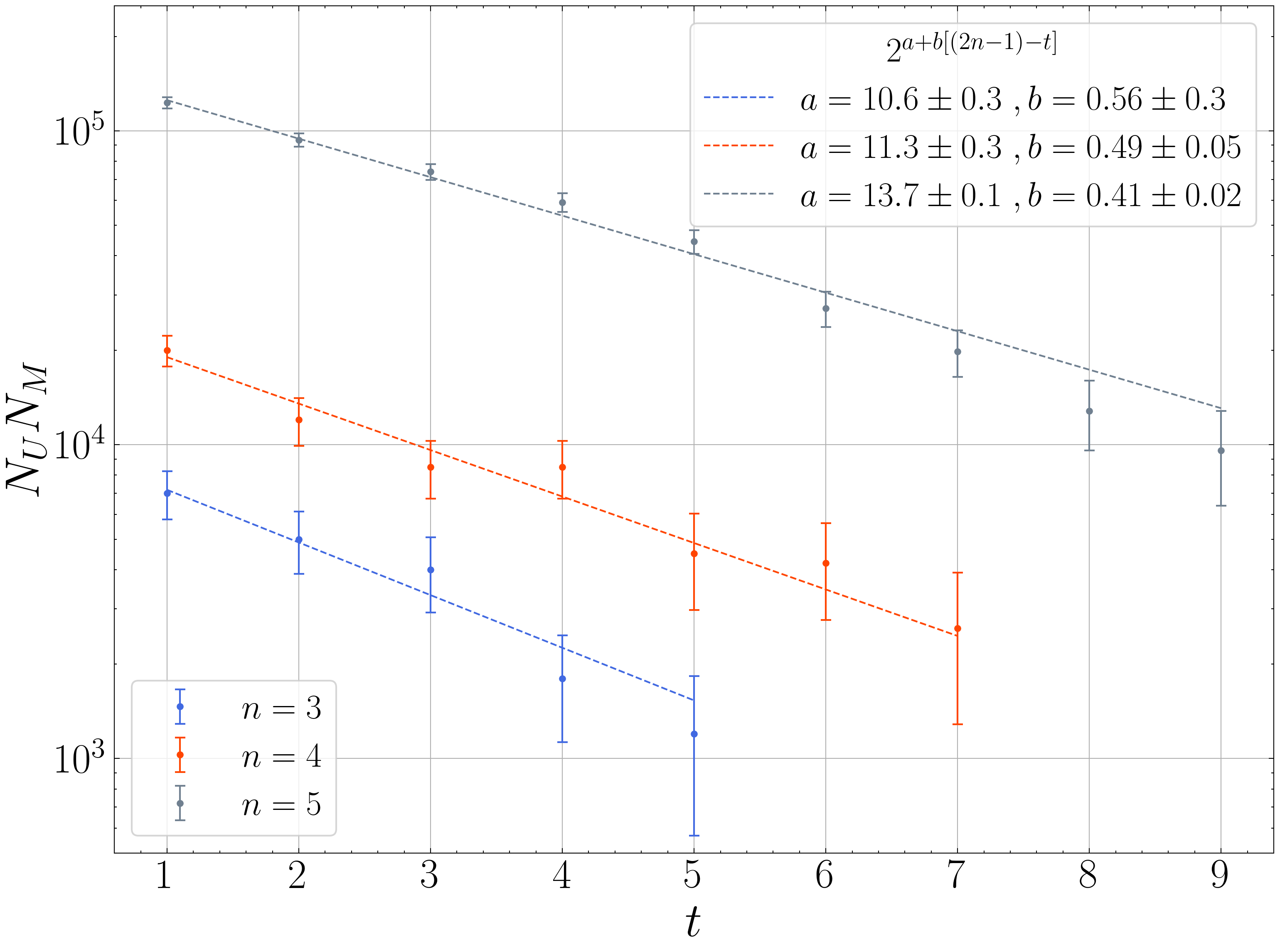
Figure 7: Number of optimal resources $N_{U}$ and $N_{M}$. The figure shows the log-plot of the optimal number of resources $N_{TOT}=N_{U}\times N_{M}$ for $n=3$ (blue dots), $n=4$ (orange dots) and $n=5$ (grey dots) as a function of the number of $T$-gates $t$ injected in the circuit. The dashed lines represent the fit $N_{TOT}=2^{a+b[(2n-1)-t]}$; the values for $a$ and $b$ with the respective errors are reported in the bottom-left corner. The fitted curves are in perfect agreement with the experimental data, whose error bars are due to the finite resolution of the grid: the $R$-squared parameters are $R^{2}_{(3)}=0.985$ for $n=3$, $R^{2}_{(4)}=0.985$ for $n=4$ and $R^{2}_{(5)}=0.995$ for $n=5$.

Data Availability The authors declare that the main data supporting the findings of this study are available within the article and its Supplementary Information files. Extra data sets are available upon reasonable request.

Acknowledgments The authors thank Benoît Vermersch, Agata Branczyk, Roberto Schiattarella, and Aurora Langella for inspiring discussions and comments. L.L., S.F.E.O. and A.H. acknowledge support from NSF award no. 2014000. The authors also thank the anonymous referees for their constructive comments and suggestions that helped to improve the manuscript. The work of L.L. and S.F.E.O. was supported in part by College of Science and Mathematics Dean’s Doctoral Research Fellowship through fellowship support from Oracle, project ID R20000000025727. S.L. was supported by DARPA, AFOSR, and ARO under a Blue Sky grant.

References

- Preskill [2018] J. Preskill, Quantum 2, 79 (2018).
- Leone et al. [2022] L. Leone, S. F. E. Oliviero, and A. Hamma, Physical Review Letters 128, 050402 (2022).
- Campbell and Browne [2010] E. T. Campbell and D. E. Browne, Physical Review Letters 104, 030503 (2010).
- Campbell [2011] E. T. Campbell, Physical Review A 83, 032317 (2011).
- Campbell et al. [2012a] E. T. Campbell, H. Anwar, and D. E. Browne, Physical Review X 2, 041021 (2012a).
- Campbell et al. [2017] E. T. Campbell, B. M. Terhal, and C. Vuillot, Nature 549, 172 (2017).
- Campbell [2014] E. T. Campbell, Physical Review Letters 113, 230501 (2014).
- Campbell and Howard [2017a] E. T. Campbell and M. Howard, Physical Review A 95, 022316 (2017a).
- Campbell and Howard [2017b] E. T. Campbell and M. Howard, Physical Review Letters 118, 060501 (2017b).
- Knill and Laflamme [1997] E. Knill and R. Laflamme, Physical Review A 55, 900 (1997).
- Gottesman [1998a] D. Gottesman, The Heisenberg Representation of Quantum Computers (1998a), arXiv:quant-ph/9807006 .
- Gottesman [1998b] D. Gottesman, Physical Review A 57, 127 (1998b).
- Aaronson and Gottesman [2004] S. Aaronson and D. Gottesman, Physical Review A 70, 052328 (2004).
- Hebenstreit et al. [2019] M. Hebenstreit, R. Jozsa, B. Kraus, S. Strelchuk, and M. Yoganathan, Physical Review Letters 123, 080503 (2019).
- Hebenstreit et al. [2020] M. Hebenstreit, R. Jozsa, B. Kraus, and S. Strelchuk, Physical Review A 102, 052604 (2020).
- Veitch et al. [2014] V. Veitch, S. A. H. Mousavian, D. Gottesman, and J. Emerson, New Journal of Physics 16, 013009 (2014).
- Howard and Campbell [2017] M. Howard and E. Campbell, Physical Review Letters 118, 090501 (2017).
- Ahmadi et al. [2018] M. Ahmadi, H. B. Dang, G. Gour, and B. C. Sanders, Physical Review A 97, 062332 (2018).
- Wang et al. [2019] X. Wang, M. M. Wilde, and Y. Su, New Journal of Physics 21, 103002 (2019).
- Seddon and Campbell [2019] J. R. Seddon and E. T. Campbell, Proceedings of the Royal Society A: Mathematical, Physical and Engineering Sciences 475, 20190251 (2019).
- Liu and Winter [2022] Z.-W. Liu and A. Winter, PRX Quantum 3, 020333 (2022).
- Seddon et al. [2021] J. R. Seddon, B. Regula, H. Pashayan, Y. Ouyang, and E. T. Campbell, PRX Quantum 2, 010345 (2021).
- White et al. [2021] C. D. White, C. Cao, and B. Swingle, Physical Review B 103, 075145 (2021).
- Qassim et al. [2021] H. Qassim, H. Pashayan, and D. Gosset, Quantum 5, 606 (2021).
- Koukoulekidis and Jennings [2022] N. Koukoulekidis and D. Jennings, npj Quantum Information 8, 1 (2022).
- Hahn et al. [2022] O. Hahn, A. Ferraro, L. Hultquist, G. Ferrini, et al., Physical Review Letters 128, 210502 (2022).
- Saxena and Gour [2022] G. Saxena and G. Gour, Physical Review A 106, 042422 (2022).
- Anwar et al. [2012] H. Anwar, E. T. Campbell, and D. E. Browne, New Journal of Physics 14, 063006 (2012).
- Campbell et al. [2012b] E. T. Campbell, H. Anwar, and D. E. Browne, Physical Review X 2, 041021 (2012b).
- Bravyi and Haah [2012] S. Bravyi and J. Haah, Physical Review A 86, 052329 (2012).
- Dawkins and Howard [2015] H. Dawkins and M. Howard, Physical Review Letters 115, 030501 (2015).
- Bravyi et al. [2016] S. Bravyi, G. Smith, and J. A. Smolin, Physical Review X 6, 021043 (2016).
- Hastings and Haah [2018] M. B. Hastings and J. Haah, Physical Review Letters 120, 050504 (2018).
- Gross et al. [2009] D. Gross, S. T. Flammia, and J. Eisert, Physical Review Letters 102, 190501 (2009).
- Beverland et al. [2020] M. Beverland, E. Campbell, M. Howard, and V. Kliuchnikov, Quantum Science and Technology 5, 035009 (2020).
- van Enk and Beenakker [2012] S. J. van Enk and C. W. J. Beenakker, Physical Review Letters 108, 110503 (2012).
- Tran et al. [2016] M. C. Tran, B. Dakić, W. Laskowski, and T. Paterek, Physical Review A 94, 042302 (2016).
- Elben et al. [2018] A. Elben, B. Vermersch, M. Dalmonte, J. I. Cirac, and P. Zoller, Physical Review Letters 120, 050406 (2018).
- Elben et al. [2019] A. Elben, B. Vermersch, C. F. Roos, and P. Zoller, Physical Review A 99, 052323 (2019).
- Vermersch et al. [2019] B. Vermersch, A. Elben, L. M. Sieberer, N. Y. Yao, and P. Zoller, Physical Review X 9, 021061 (2019).
- Brydges et al. [2019] T. Brydges, A. Elben, P. Jurcevic, B. Vermersch, C. Maier, B. P. Lanyon, P. Zoller, R. Blatt, and C. F. Roos, Science 364, 260 (2019).
- Ketterer et al. [2019] A. Ketterer, N. Wyderka, and O. Gühne, Physical Review Letters 122, 120505 (2019).
- Elben et al. [2020a] A. Elben, R. Kueng, H.-Y. R. Huang, R. van Bijnen, C. Kokail, M. Dalmonte, P. Calabrese, B. Kraus, J. Preskill, P. Zoller, and B. Vermersch, Physical Review Letters 125, 200501 (2020a).
- Knips et al. [2020] L. Knips, J. Dziewior, W. Kłobus, W. Laskowski, T. Paterek, P. J. Shadbolt, H. Weinfurter, and J. D. A. Meinecke, npj Quantum Information 6, 51 (2020).
- Ketterer et al. [2022] A. Ketterer, S. Imai, N. Wyderka, and O. Gühne, Physical Review A 106, L010402 (2022).
- Zhou et al. [2020a] Y. Zhou, P. Zeng, and Z. Liu, Physical Review Letters 125, 200502 (2020a).
- Cian et al. [2021] Z.-P. Cian, H. Dehghani, A. Elben, B. Vermersch, G. Zhu, M. Barkeshli, P. Zoller, and M. Hafezi, Physical Review Letters 126, 050501 (2021).
- Imai et al. [2021] S. Imai, N. Wyderka, A. Ketterer, and O. Gühne, Physical Review Letters 126, 150501 (2021).
- Rath et al. [2021] A. Rath, R. van Bijnen, A. Elben, P. Zoller, and B. Vermersch, Physical Review Letters 127, 200503 (2021).
- IBM Quantum [2021] IBM Quantum, https://quantum-computing.ibm.com/(2021).
- Zhou et al. [2020b] S. Zhou, Z.-C. Yang, A. Hamma, and C. Chamon, SciPost Physics 9, 87 (2020b).
- Leone et al. [2021] L. Leone, S. F. E. Oliviero, Y. Zhou, and A. Hamma, Quantum 5, 453 (2021).
- Oliviero et al. [2021] S. F. Oliviero, L. Leone, and A. Hamma, Physics Letters A 418, 127721 (2021).
- Elben et al. [2020b] A. Elben, B. Vermersch, R. van Bijnen, C. Kokail, T. Brydges, C. Maier, M. K. Joshi, R. Blatt, C. F. Roos, and P. Zoller, Physical Review Letters 124, 010504 (2020b).
- Elben et al. [2020c] A. Elben, J. Yu, G. Zhu, M. Hafezi, F. Pollmann, P. Zoller, and B. Vermersch, Science Advances 6, eaaz3666 (2020c).