Recovering models of open quantum systems from data via polynomial optimization: Towards globally convergent quantum system identification

Abstract

Current quantum devices suffer imperfections as a result of fabrication, as well as noise and dissipation as a result of coupling to their immediate environments. Because of this, it is often difficult to obtain accurate models of their dynamics from first principles. An alternative is to extract such models from time-series measurements of their behavior. Here, we formulate this system-identification problem as a polynomial optimization problem. Recent advances in optimization have provided globally convergent solvers for this class of problems, which using our formulation prove estimates of the Kraus map or the Lindblad equation. We include an overview of the state-of-the-art algorithms, bounds, and convergence rates, and illustrate the use of this approach to modeling open quantum systems.

I Introduction

Quantum technologies [1, 2], which rest on the ability to actively control microscopic systems and exploit their unique quantum mechanical features, have the potential for high impact in a number of different fields; from precision sensing [3, 4, 5] and communication [6, 7], to encryption [8] and very prominently quantum computing [1, 9, 10]. The extreme sensitivity of quantum effects to their immediate environment, combined with the exquisite control required to exploit these effects, necessitates accurate dynamical modeling. However, fabrication imperfections and the complex nature of the environment often make it impossible to obtain an accurate dynamical description from first principles. Because of this, one must determine a sufficiently accurate model from measurements of the quantum system. In machine learning and control engineering, this task is referred to as system identification [11].

In the quantum technology community, system identification tools are used to better understand, characterize, and benchmark quantum devices, and in certain contexts are referred to as quantum process tomography [1, Chapter 8]. More precisely, the goal of quantum process tomography is to reconstruct a description of a quantum process from the measurement outcomes of the expectation values of certain operators, which are sampled uniformly. The measurements fed into the SID algorithms can be obtained in a number of different ways. Most often, they are given as the outputs of quantum state tomography, where one usually prepares or initializes several identical copies of the input quantum states (probe states) $\rho_{0}$, which evolve according to some unknown quantum process $\mathcal{P}$ which is sampled and results in measuring expectation values $\langle O_{i}\rangle$ with respect to a complete set of Hermitian operators $\{O_{i}\}$, see Fig. 1. In this way, one can reconstruct the evolved state which will be used in the quantum system identification algorithms [1].

Several methods have been developed for identifying quantum systems in various contexts [12, 13, 14, 15, 16, 17, 18, 19, 20, 21, 22, 23] including approaches based on active learning [24]. These approaches may involve starting the system from a set of initial states and then making measurements at a given final time, with the purpose of determining the linear map from the initial to the final time. Here, we are also interested in obtaining the dynamical equations of motion for the system. Without an interaction with the environment, the quantum evolution is completely captured by the Hamiltonian $H$ of the system. When there is an environmental component, the system is referred to as being “open” and the evolution is given by a “master equation” whose form is constrained by the need to conserve the trace and positivity of the density matrix $\rho$. The first constraint is particularly important since the preservation of the unit trace of the density matrix in particular is important because it implies the probability preservation of the quantum system. However, in numerical integration schemes the requirements for positivity are slightly relaxed, due to the nature of these numerical methods and due to the dissipative nature of open quantum systems.

In the references cited above, mainly closed (Hamiltonian) quantum systems were considered. However, especially in the NISQ era of quantum technologies [25], noise is abundant. In practice, a quantum device is never completely isolated. Thus, one has to identify the open quantum systems [1, 26, 27].

Several methods have been proposed to determine master equations of open quantum systems from time-series data. For example, Zhang and Sarovar drew on the linear system identification theory to create a method for obtaining parameters of parametrized Hamiltonians and master equations from time-series [28]. McCauley et al. used a linear SID method to obtain minimal models of open systems [29]. The core element of these methods is the singular value decomposition of a matrix constructed from the data.

More recently, Samach et. al. [20] designed a technique for extracting the Hamiltonian, jump operators, and corresponding decay rates in open quantum systems, with the aim of characterizing superconducting qubit platforms. Closely related to the current paper is the work of Xue et. al. [21] who proposed a method for obtaining parametrized master equations for open quantum systems based on the following steps: (1) Collect time series measurements $D_{N}$ of the evolution of the density matrix of the system of interest. (2) Define a parametrized model for the system and estimate the evolution. (3) Define a cost function and optimize it taking into account possible constraints. Update the parameters accordingly. (4) If the error satisfies the desired criteria, stop. Otherwise, adjust the model accordingly. The algorithms of both Samach et. al. and Xue et. al. concern open quantum systems with Markovian dynamics, which are described by the master equation in terms of the Lindblandian operator $\mathcal{L}$ (see Sec. II). In [20], maximum likelihood estimation is used while [21] uses the full exponential of the Landbladian where after defining a cost function they apply a gradient step, where the gradient is with respect to the parameters of the Hamiltonian. This procedure resembles common machine learning techniques for recovering the dynamics of open quantum systems, e.g. [30].

In this paper, we assume an open quantum system with both arbitrary dissipative dynamics described by Kraus operators and Markovian dynamics described by a Lindbland master equation. We use time series $D_{N}$ as obtained, e.g., by quantum state tomography. However, with the aim of being as generic as possible, we chose not to parametrize the Hamiltonian of the system, leaving it arbitrary, as we do with the jump operators. Furthermore, using certain approximations for the evolution operator $\exp(\mathcal{L}\Delta t)$, where $\Delta t$ is the chosen time step, we can cast the problem as a polynomial optimization problem, unlike previous approaches [20, 21]. This is particularly important because

• Formulating the problem as a polynomial optimization problem opens the door to utilizing methods with proven guarantees of global asymptotic convergence.

• Our numerical illustrations show that even quasi-Newton methods on one of our formulations converged in all $1.06\times 10^{3}$ tests carried out.

To appreciate the significance of point (2) above, consider the fact that optimization algorithms based on first-order methods, including the quasi-Newton ones utilized in the numerical illustration of this paper, are heuristic, in the sense that they can diverge or converge to arbitrarily poor solutions, when applied to a non-convex optimization problem without further structure. Therefore, no guarantees about their global convergence can be provided. On the other hand, the semialgebraic sets we consider in the polynomial optimization problems are tame (definable in o-minimal structure, [31]) by definition. Recent studies [32] have shown certain first-order methods to be well behaved when the graph of the function is tame [32]. This observation may be of independent interest.

To appreciate the significance of point (1) above, note that for a single formulation of the problem, multiple methods without guarantees of global convergence may produce multiple estimates of the open quantum system, especially when starting from multiple initial solutions. This has an impact on any subsequent uses of the estimates. Consider, for example, the uses of the estimates in quantum optimal control [33, 34]. An imprecise estimate of the open quantum system may lead to poor quality control signals, which in turn lead to low-fidelity 2-qubit gates [35] or poor outcomes in the laser control [36] of chemical reactions. In contrast, the guarantees of global asymptotic convergence for the optimization over semi-algebraic sets make it possible to obtain the best possible estimates.

Figure 1: An unknown quantum process $\mathcal{P}$ characterizing some device can be estimated and identified by making experiments involving several copies of input states and collecting data on the expectation values of certain operators $O_{i}$. The measured data can be used in order to construct the empirical estimate $\mathds{E}[O_{i}]$ of the expectation value $\langle O_{i}\rangle$. For a closed quantum system $\mathcal{P}$ is a unitary operator, while for an open system it is assumed to correspond to a Hermitian matrix.

Notation

The imaginary unit is denoted as $\operatorname{\mathring{\imath}}\coloneqq\sqrt{-1}$ while $i$ is reserved for the sample indexing of the measurement time series $D_{N}$. We denote by $\|A\|_{F}\coloneqq\sqrt{\Tr(AA^{\dagger})}$ the Frobenius norm of a matrix $A$, while by $\hat{A}$ we denote the estimate of $A$.

II Set up

Most often, one considers a quantum system of interest composed of smaller subsystems. In general, the evolution of this combined dissipative quantum system, in state $\rho$, is described by a process $\mathcal{P}:\rho(0)\to\rho(t)$ formulated in terms of the CPTP Kraus map operator sum representation [1]

$$\rho(t) =\sum_{k=1}^{\ell}E_{k}\rho(0)E_{k}^{\dagger}.$$ (1)

The operators $\{E_{k}\}_{k=1}^{\ell}$ are called Kraus operators and satisfy the completeness relation $\sum_{k=1}^{\ell}E_{k}^{\dagger}E_{k}=\mathds{1}$ with $\ell\leq n^{2}-1$. The process responsible for Eq. (1) is linear, preserves the trace and hermiticity, and corresponds to a positive map. Additionally, the super-operator $\mathcal{P}$, also known as the process, can be considered as the carrier of noise due to the exchange of energy with the bath surrounding the quantum system of interest. For the reasons described in Sec. I, we are interested in algorithmic procedures that identify such processes $\mathcal{P}$.

A natural question to ask is whether $\mathcal{P}$ is identifiable in the first place. This question motivated Wang et. al. to define the notion of quantum identifiability [19] using similarity transformations. However, this work focuses on the case of continuous evolution. Practically, and as will be described in the following, one can only work in the discrete domain, that is, to consider the discrete-time stroboscopic evolution of the open quantum system. The notion of identifiability for this case is defined and analyzed in [37].

Assuming that discrete quantum identifiability holds, one can attempt to perform system identification of $\mathcal{P}$ for open quantum systems by finding a set of Kraus operators $\{\hat{E}_{k}\}_{k=1}^{\ell}$ modeling the dynamics of open quantum systems, that is, they describe the evolution of the initial state $\rho$ in the data $D_{N}$. Here, $\hat{E}_{k}$ denote the search variables that estimate ${E}_{k}$. Specifically, using state reconstruction techniques, such as quantum state tomography, one can obtain empirical estimates of the state of the total system at time $t$. When uniformly sampling the process $\mathcal{P}$ a total $N$ times such that $t=N\Delta t$, one obtains a time series $D_{N}=\{\rho_{(0)},\ldots\rho_{(N)}\}$. For a given time sample $i$, the evolution of $\rho_{(i)}$ by $\Delta t$ yields $\rho_{(i+1)}$, i.e.,

$$\mathcal{P}:{\rho}_{(i)}\mapsto{\rho_{(i+1)}},$$ (2)

for all $i=0,1,\ldots,N$.

III System Identification for the Kraus-Map

Given the description of the quantum open system as described in Eq. (1), as well as the quantum identifiability assumption, the task to be performed amounts to finding the Kraus operators that recover the time evolution of the density matrix that is closest to the data $D_{N}$, providing the best estimate for $\mathcal{P}$. Given a single input and output state, a natural formulation yields the following optimization problem —l— ^E_k ∥ ∑_k=1^ℓ^E_k ρ_(0) ^E_k^† - ρ_(1) ∥_F^2 ∑_k=1^ℓ^E_k^†^E_k = 1.

In this optimization problem, we have chosen as an objective function the Frobenius norm between the measured sample $\rho_{0}$ and the estimated one $\hat{\rho}_{1}=\sum_{k=1}^{\ell}\hat{E}_{k}\rho_{0}\hat{E}_{k}^{\dagger}$. Taking into account the time series $D_{N}$ in its entirety, one generalizes the objective to —l— ^E_k ∑_i=0^N-1 ∥ ∑_k=1^ℓ^E_k ρ_(i) ^E_k^† - ρ_(i+1) ∥_F^2 ∥ ∑_k=1^ℓ^E_k^†^E_k -1 ∥_F^2 = 0.

In closing this section, it is worth mentioning that an approach to consider is to perform a linearization of the system, similar to [38, 19]. In [37], starting from the Kraus representation, a linearization of the discretized system is considered to allow the reformulation of Prob. (III) as a linear dynamical system, and it is shown that using noncommutative polynomial optimization, the problem can be attacked using a series of convergent relaxations. Furthermore, under certain tameness assumptions, as well as assumptions on the dimensions of the density matrices, the problem can be attacked using standard gradient-like methods.

IV System identification for Lindblad master equations

For certain applications within quantum optics [39] and cavity quantum electrodynamics [40], both being very relevant as different approaches for current NISQ and future FTEC quantum devices, as well as optomechanic applications [41], the Lindblad master equation is a widely popular theoretical tool for modeling open quantum system dynamics. The Lindblad equation (also known as the Gorini-Kossakowski-Sudarshan-Lindblad equation) [42, 43] reads

$$\frac{d}{dt}{\rho}(t)=\mathcal{L}\rho(t),$$ (3)

where the Lindbladian operator is given as

$$\mathcal{L}[\rho]=\frac{\operatorname{\mathring{\imath}}}{\hbar}[H,\rho]+\sum_{j=1}^{\ell}\left[2A_{j}\rho A_{j}^{\dagger}-\left\{A_{j}^{\dagger}A_{j},\rho\right\}\right],$$ (4)

where $H$ is the Hamiltonian and the set $\{A_{j}\}$ are called jump operators describing the dampening of the system.

Sections IV.1 and IV.2 below present two fundamentally different ways of formulating the identification problem for Eq. (3) in terms of polynomial optimization.

IV.1 The Padé method

Exponentiating the Lindblad operator (4) one obtains the process mapping (2) such that the recorded time series $D_{N}$ can be written as

$${\rho}_{(i+1)}=e^{\Delta t\mathcal{L}}{\rho_{(i)}},\quad i=0,1,\ldots,N.$$ (5)

In the context of the Lindblad master equation, therefore, identifying the process $\mathcal{P}$ amounts to recovering the operators of the master equation that predict the evolution of the open quantum system closest to the data. In other words, in this context, identifying $\mathcal{P}$ amounts to finding an estimate $\hat{\mathcal{L}}$ of the linear operator $\mathcal{L}$ that fits the best with the data $D_{N}$ that correspond to the evolution of the density matrix.

The exponent in Eq. (5) can be rewritten as

$$e^{\Delta t\mathcal{L}}=\frac{\mathds{1}+\tanh(\Delta t\mathcal{L}/2)}{\mathds{1}-\tanh(\Delta t\mathcal{L}/2)}$$ (6)

and by Taylor expanding $\tanh$, one obtains the Padé approximation

$$e^{\Delta t\mathcal{L}}=\frac{\mathds{1}+\Delta t\mathcal{L}/2}{\mathds{1}-\Delta t\mathcal{L}/2}+\mathcal{O}(\Delta t^{3}),$$ (7)

that can be used to linearize the problem of identifying $\mathcal{P}$. Note that this is equivalent to the 1st-order Padé approximation [44] (closely related to the Cayley transform), which explicitly preserves unitary in the case $A_{j}=0$. Linearization of the same problem is also considered in [19] in the continuous case, as well as in [37] in the discrete case, but in both cases approaching the problem from the Kraus map perspective described in Section III.

Substituting the Padé approximation (7) into Eq. (5), we obtain

$$\left(\mathds{1}-\Delta t\mathcal{L}/2\right){\rho}_{(i)} =(\mathds{1}+\Delta t\mathcal{L}/2){\rho}_{(i-1)}+\mathcal{O}(\Delta t^{3}),\$$

which can be further simplified to

$${\rho_{(i)}-\rho_{(0)}-\Delta t\mathcal{L}\left[\frac{{\rho}_{(i)}+{\rho}_{(i-1)}}{2}\right]} =\mathcal{O}(\Delta t^{3}).$$ (8)

Following the steps that led to the formation of Prob. (III), up to $\mathcal{O}(\Delta t^{3})$ errors, the identification of Lindblandian (4) from the time-trace of density matrices $D_{N}$ is reduced to the following unconstrained polynomial optimization problem —l— A_j, H∑_j=1^N ∥ ρ_(i) - ρ_(i-1) - Δt L [ρ(i)+ ρ(i-1)2 ] ∥_F^2 .

IV.2 The integral method

A very different approach is obtained if the master equation (3) is integrated over the time interval $[t_{0},t_{i}]$,

$$\rho_{(i)}-\rho_{(0)} =\int_{t_{0}}^{t_{i}}\frac{d}{dt}{\rho}(t)dt=\int_{t_{0}}^{t_{i}}\!\!\!\mathcal{L}[\rho(t)]dt$$

$$=\mathcal{L}\left[\int_{t_{0}}^{t_{i}}\!\!\!\rho(t)dt\right].$$ (9)

The uniform discretization of the integration domain $[0,t]$, by sampling the process $N$ times, yields the formulation for the identification of Lindblandian (4) as the following unconstrained polynomial optimization problem —l— A_j, H∑_i=1^N ∥ ρ_(i) - ρ_(0) - L [∫^iΔt_0ρ(t)dt ] ∥ ^2_F . Given the time series $D_{N}$, the integral can be readily evaluated, e.g., within $\mathcal{O}(\Delta t^{2})$ accuracy via the trapezoidal rule and within $\mathcal{O}(\Delta t^{4})$ accuracy via Simpson’s rule. However, as will be shown in Sec. VI, despite the fact that the Padé  (IV.1) has a lower asymptotic accuracy of $\mathcal{O}(\Delta t^{3})$ , in practice it outperforms Simpson’s method.

V System Identification as Polynomial Optimization

The formulations of the open system identification problem above are natural and easy to interpret, but to a non-expert, it may not be obvious how to solve those problems. Crucially, the formulations of the problem of Hamiltonian identification as in Probs. (III) and (IV.1), (IV.2) correspond exactly to polynomial optimization problems, which form one of the broadest classes of non-convex optimization problems, for which we have (asymptotic) guarantees of convergence to the global optima.

While it is common to rely to first-order heuristic methods, such as the gradient descent, this might not be always sensible, especially if no tameness assumptions on the algebraic structure of the feasible sets are made. In such cases, one might run into common problems associated with first-order methods, for example, suboptimal solutions or divergence. Nevertheless, the global optimum can be estimated to any precision using newly developed hierarchies of convexifications. The development of such algorithms is a rapidly growing field. In Table 1, we summarize several such methods for solving polynomial optimization methods as well as their convergence guarantees. We provide an overview of the mathematical structure of such globally convergent methods in the Supplementary material. In particular, Appendix A presents an overview of the state-of-the-art algorithms for solving either Prob. (III), Prob. (IV.1) or Prob. (IV.2) using hierarchies of convexifications, which guarantee convergence to global optima of polynomial optimization problems.

Year	Method	Reference				Convergence guarantees
1970	Broyden-Fletcher-Goldfarb-Shanno	Broyden et al. [46, 47, 48, 49]				None
2001	Moment/SOS	Lasserre [50] and Parillo [51]				Asymptotic
2006	Sparse variants of Moment/SOS	Kojima et al. [52] and Lasserre [53, 54]				Asymptotic
2016	Bounded-degree SOS (BSOS)	Lasserre et al. [55]				Asymptotic
2019	Nonnegative circuit polynomials	Dressler et al. [56]				Asymptotic
2018	Piece-wise linear approx.	Long history [57]				Asymptotic
2021	Lasserre’s spectral	Lasserre [58]				Bounded rate [59]
2021	Second-order-cone approx. (DSOS)	Ahmadi and Majumdar [60]				None [61]
2021	Relative-entropy relaxations	Chandrasekaran et al. [62, 63]				Asymptotic
2022	Using Putinar’s Positivstellensatz	Roebers et al. [64]				Asymptotic
2022	Quadrature-based methods	Piazzon et al. [65, 66, 67]				Bounded rate [67]

Table 1: A selection of commutative polynomial optimization methods. See Table 2 for their implementations.

VI Computational Illustrations

To illustrate the identification methods presented in Sects. III and IV, we run in total over $340\times 10^{3}$ tests. The statistics obtained are visualized in Fig. 2. For every test, we i) randomly generate open quantum systems, ii) obtain a time trace, iii) run a polynomial optimization algorithm to identify a model from the time trace, and finally, iv) compare the known system with the identified model. Let us describe every stage of this pipeline in detail.

To generate a time series $D_{N}$ of $2\times 2$ density matrices, we first randomly generate a Hamiltonian $H$, (using the function rand_herm from the Python library qutip [68, 69]), an initial state $\rho^{\rm exact}_{(0)}$ (via qutip.rand_dm), and a non-Hermitian jump operator $A_{1}$. Then, the Lindblad master equation (3) and (4) ($\ell=1$) is solved to generate a time series of 50 density matrices using qutip.mesovle. To mimic experimental noise, for each density matrix $\rho^{\rm exact}$ of the time series, a random density matrix $\rho^{\rm rand}$ is admixed as follows:

$$\rho^{\rm noisy}_{(i)}= (1-w)\rho^{\rm exact}_{(i)}+w\rho^{\rm rand}_{(i)},$$ (10)

$$0\leq w<1,\quad i=0,\ldots,N,$$

to form the final time series $D_{N}$ ($N=49$) that is then used for identification. In Eq. (10), $w$ is a mixing coefficient, which quantifies the magnitude of noise: The higher $w$, the noisier the time series is. Note that by construction $\rho_{(i)}^{\rm noisy}$ is non-negative.

The polynomial objective functions (III), (IV.1), (IV.2) and their gradients are computed from the time series $D_{N}$ by using the Python library sympy [70].

First, we considered an encoding of the polynomial optimization problems in ncpol2sdpa. However, the size of the SDP instances would result in a vast carbon footprint. Therefore, the optimization was performed using a local optimization method implemented in scipy.optimize. In particular, we have used the implementation of the basin-hopping algorithm [71] version of the Broyden-Fletcher-Goldfarb-Shanno (BFGS) quasi-Newton method [46, 47, 48, 49], which is the first row of Table 1. Essentially, this is a global stepping algorithm with local minimization via a modified gradient descent.

Having solved the corresponding polynomial minimization, we identify a model of the open quantum system. To quantify the accuracy of the identification, we use the minimum fidelity $F_{\min}$ between the exact and identified time series, which is calculated in two steps: First, the backed-out model is used to propagate the known initial condition $\rho^{\rm noisy}_{(0)}$ to obtain the identified time series $\rho^{\rm sid}_{(i)}$, $i=0,\ldots,N$, $\rho^{\rm sid}_{(0)}=\rho^{\rm noisy}_{(0)}$. The index $i$ labels the same time moments here and in Eq. (10). Second, we evaluate $F_{\min}$ as

$$F_{\min} =\min_{i=0,\ldots,N}F\left(\rho^{\rm exact}_{(i)},\rho^{\rm sid}_{(i)}\right),$$ (11)

$$F\left(\rho^{\rm exact}_{(i)},\rho^{\rm sid}_{(i)}\right) =\Tr\sqrt{\sqrt{\rho^{\rm exact}_{(i)}}\rho^{\rm sid}_{(i)}\sqrt{\rho^{\rm exact}_{(i)}}}.$$ (12)

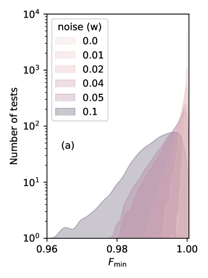
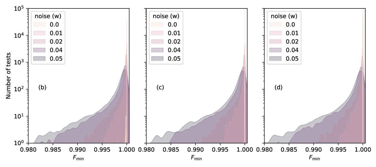
Figure 2: Distributions of fidelity $F_{\min}$ (11) for open quantum system identification as a function of the noise mixing coefficient $w$ (10). ($w=0$ is the noiseless case.) (a) The fidelity distribution for the Kraus map identification method (III). The fidelity distribution for the Lindblad master equation identification problem via (b) the Padé method (IV.1) and the integral formulation (IV.2) where the integral is estimated via (c) the trapezoidal and (d) Simpson’s rules.

Figure 2 displays the minimum fidelity distribution for the tests of (a) the Kraus map identification, the Lindblad master equation identification via (b) the Padé, (c) trapezoidal, and (d) Simpson methods. The figure also demonstrates the robustness to noise of the developed methods.

It is noteworthy that the algorithm converged to the minimum of the polynomial optimization problem for every attempted test of the Kraus map identification problem (III) [Figs. 2(a)] as well as the Padé formulation (IV.1) of the Lindblad equation identification problem [Figs. 2(b)]. In contrast, the basin-hopping algorithm did not converge in half of cases (irrespective of noise) for the integral formulations of the trapezoid and Simpson integral formulations (IV.2) of the Lindblad equation identification problem. Hence, Figs. 2(c, d) visualize only the converged tests.

VII Conclusions

We have demonstrated globally convergent methods for the estimation of Kraus maps and Lindblad master equations directly from time series data by formulating the problem as a polynomial optimization problem. We discussed in detail the benefits of the polynomial optimization formulation and explained methods for obtaining global optima. Improved estimates of models of open quantum systems should, in turn, allow for improved pulse shaping for 2-qubit gates [35] and improved error cancellation [72].

Our work here starts with the results of quantum state tomography. Instead, one could start at the readout-pulse level [73] or with randomized measurements [23]. This seems to open up further important applications of polynomial optimization in quantum information science.

Appendix A Polynomial optimization illustrated

Environment	Library	Methods	Solver
Python	Irene	[50, 51]	DSDP5
	ncpol2sdpa	[50, 51]	Mosek
Julia	SumOfSquares.jl	[50, 51]	NAG
	PolyJuMP.jl	[50, 51]	PENNON
	TSSOS	[75]	PENLAB
	CS-TSSOS	[75, 76]	COSMO
MATLAB	YALMIP	[50, 51]	SDPNAL+
	REPOP	[62, 63]	ECOS
	SOSTOOLS	[50, 51]	SCS
	SparsePOP	[52, 53, 54]	SDPA
	GloptiPoly	[50, 51]	Sedumi

Table 2: A small selection of available modeling languages and SDP solvers. Note that most of the modeling languages support multiple SDP solvers, although Sedumi, CDCS, and SDPNAL+ are restricted to MATLAB environment. For further relaxations, see Table 1.

In this section, we present a technical overview of the state-of-the-art algorithms for solving polynomial optimization problems, such as Prob. (III), Prob. (IV.1) and Prob. (IV.2). Most of these approaches build up a hierarchy of relaxations, i.e., auxiliary problems whose objective functions monotonically increases and provides progressively improving lower bounds on the true objective function. This can be interpreted as a procedure, where one augments the search space in a way that convexifies it and then step by step starts shrinking it again such that at some point, the relaxations become sufficient to extract the global optimizer, i.e., the solution which attains the global optimum in terms of the objective function value. A crucial aspect of the approaches summarized is the rate of growth of the (dimensions, numbers, and dimension of constraints in the) relaxations within the hierarchy and the rate of growth of the lower bounds provided by the relaxations.

Broadly speaking, all of these approaches are based on various Positivstellensätze to form the relaxations. In real algebraic geometry, Positivstellensätze characterize polynomials that are positive on a semialgebraic set, which can be thought of as real analogues of Hilbert’s Nullstellensatz. (These are sometimes known as sum-of-squares representation theorems.) Using Putinar’s Positivstellensatz [77], Lasserre obtained his original hierarchy, while others have used it to obtain the SOCP hierarchies [64]. Using Krivine–Stengle Positivstellensatz [78] has yielded a linear programing hierarchy of historic importance and the more recent BSOS hierarchy [55]. Using Schmüdgen’s Positivstellensatz [79], one be used to obtain the SOCP hierarchy. Generally, each Positivstellensatz can yield multiple hierarchies of relaxations of various properties. See the Supplementary material for further illustrations.

For example, let us consider the moment/SOS hierarchy of semidefinite relaxations [50, 51] (see [80] for a survey) are applied to polynomial optimization problems such as Prob. (III). The idea behind moment/SOS relaxations is to use the so-called moment and localizing matrices that, at each higher order, by appropriately amplifying and essentially convexifying the search space, they approximate better the actual non-convex problem one is interested in solving. In particular, the moment/SOS approaches of Lasserre and Parrilo are based on probability density measures $\mathcal{M}(\mathds{R}^{n})$ and polynomials over $\mathds{R}[\bm{x}],\,\bm{x}\in\mathds{R}^{n}$, respectively. In Prob. (III), one needs to impose the Archimedean property [81], which states that a semi-algebraic set $K$, defined as

$$K:=\left\{\bm{x}\in\mathds{R}^{n}|p_{i}(\bm{x})\geq 0\text{ and }h_{j}(\bm{x})=0,\,\forall i,j\right\},$$ (13)

for polynomials $\{p_{i}\}_{i=1}^{m}\in\mathds{R}[\bm{x}]$ and $\{h\}_{j=1}^{r}\in\mathds{R}[\bm{x}]$, is associated with the quadratic module $M(g;h)=M\left(g_{1},\ldots g_{m};h_{1},\ldots,h_{r}\right)\subset\mathds{R}[\bm{x}]$, a subring of $\in\mathds{R}[\bm{x}]$ defined as the set of polynomials that can be written in the form

$$\sigma_{0}+\sum_{j=1}^{m}\sigma_{j}(\bm{x})p_{j}(\bm{x})+\sum_{j=1}^{r}\phi_{j}(\bm{x})h_{j}(\bm{x})$$

where $\{\sigma_{j}\}_{j=0}^{m}\subset\mathds{R}[\bm{x}]$ are sum-of-square polynomials and $\{\phi\}_{j=1}^{r}\subset\mathds{R}[\bm{x}]$.

Figure 3: A graphical summary of some of the reformulations of polynomial optimization and their relaxations: two columns in the middle suggest the Moment/SOS hierarchy [50, 51], which is best known. To the right, the so called relative-entropy relaxations [62, 63] based on the sums of arithmetic-geometric-exponentials (SAGE) decompositions. The bended arrows denote inclusions. See Table 1 for further relaxations.

When dealing with the constrained Prob. (III), the Archimedean condition must be assumed. This is, however, not the case with Prob. (IV.1) and Prob. (IV.2).

A graphical summary of the architecture of the Moment/SOS relaxation routines is provided in Figure 3.

Many extensions of the moment/SOS relaxations have been developed, some of those as well other algorithmic approaches are summarized in Table 1.

For the benefit of practitioners, in Table 1, we list a collection of libraries for Python, Julia, and MATLAB that implement the hierarchies of convexifications described previously. These can be used in the context of open quantum system identification to yield globally optimal results. In the same table, we further list a small subset of the publicly available solvers. Note that the last column (Solver) is independent to the previous ones, in the sense that the rows of the last column do not mean there is a one-to-one correspondence with the row of the previous columns.

References

- Michael A. Nielsen [2011] I. L. C. Michael A. Nielsen, Quantum Computation and Quantum Information: 10th Anniversary Edition, 10th ed. (Cambridge University Press, 2011).
- Ezratty [2021] O. Ezratty, Understanding quantum technologies (2021).
- Yu et al. [2021] Q. Yu, Y. Wang, D. Dong, and I. R. Petersen, On the capability of a class of quantum sensors, Automatica 129, 109612 (2021).
- Xie et al. [2022] M. Xie, X. Yu, L. V. H. Rodgers, D. Xu, I. Chi-Durán, A. Toros, N. Quack, N. P. de Leon, and P. C. Maurer, Biocompatible surface functionalization architecture for a diamond quantum sensor, Proceedings of the National Academy of Sciences 119, e2114186119 (2022), https://www.pnas.org/doi/pdf/10.1073/pnas.2114186119 .
- Marciniak et al. [2022] C. D. Marciniak, T. Feldker, I. Pogorelov, R. Kaubruegger, D. V. Vasilyev, R. van Bijnen, P. Schindler, P. Zoller, R. Blatt, and T. Monz, Optimal metrology with programmable quantum sensors, Nature 603, 604 (2022).
- Luo et al. [2019] Y.-H. Luo, H.-S. Zhong, M. Erhard, X.-L. Wang, L.-C. Peng, M. Krenn, X. Jiang, L. Li, N.-L. Liu, C.-Y. Lu, A. Zeilinger, and J.-W. Pan, Quantum teleportation in high dimensions, Phys. Rev. Lett. 123, 070505 (2019).
- Liao et al. [2018] S.-K. Liao, W.-Q. Cai, J. Handsteiner, B. Liu, J. Yin, L. Zhang, D. Rauch, M. Fink, J.-G. Ren, W.-Y. Liu, Y. Li, Q. Shen, Y. Cao, F.-Z. Li, J.-F. Wang, Y.-M. Huang, L. Deng, T. Xi, L. Ma, T. Hu, L. Li, N.-L. Liu, F. Koidl, P. Wang, Y.-A. Chen, X.-B. Wang, M. Steindorfer, G. Kirchner, C.-Y. Lu, R. Shu, R. Ursin, T. Scheidl, C.-Z. Peng, J.-Y. Wang, A. Zeilinger, and J.-W. Pan, Satellite-relayed intercontinental quantum network, Phys. Rev. Lett. 120, 030501 (2018).
- Grasselli [2021] F. Grasselli, Quantum Cryptography (Springer International Publishing, 2021).
- O’Brien et al. [2009] J. L. O’Brien, A. Furusawa, and J. Vučković, Photonic quantum technologies, Nature Photonics 3, 687 (2009).
- Huggins et al. [2022] W. J. Huggins, B. A. O’Gorman, N. C. Rubin, D. R. Reichman, R. Babbush, and J. Lee, Unbiasing fermionic quantum monte carlo with a quantum computer, Nature 603, 416 (2022).
- Simpkins [2012] A. Simpkins, System identification: Theory for the user, 2nd edition, IEEE Robotics & Automation Magazine 19, 95 (2012).
- Geremia and Rabitz [2002] J. M. Geremia and H. Rabitz, Optimal identification of hamiltonian information by closed-loop laser control of quantum systems, Phys. Rev. Lett. 89, 263902 (2002).
- Howard et al. [2006] M. Howard, J. Twamley, C. Wittmann, T. Gaebel, F. Jelezko, and J. Wrachtrup, Quantum process tomography and linblad estimation of a solid-state qubit, New Journal of Physics 8, 33 (2006).
- Le Bris, Claude et al. [2007] Le Bris, Claude, Mirrahimi, Mazyar, Rabitz, Herschel, and Turinici, Gabriel, Hamiltonian identification for quantum systems: well-posedness and numerical approaches, ESAIM: COCV 13, 378 (2007).
- Guta and Yamamoto [2016] M. Guta and N. Yamamoto, System identification for passive linear quantum systems, IEEE Transactions on Automatic Control 61, 921–936 (2016).
- Sone and Cappellaro [2017] A. Sone and P. Cappellaro, Hamiltonian identifiability assisted by a single-probe measurement, Physical Review A 95, 10.1103/physreva.95.022335 (2017).
- Wang et al. [2018] Y. Wang, D. Dong, B. Qi, J. Zhang, I. R. Petersen, and H. Yonezawa, A quantum hamiltonian identification algorithm: Computational complexity and error analysis, IEEE Transactions on Automatic Control 63, 1388 (2018).
- Aaronson et al. [2019] S. Aaronson, X. Chen, E. Hazan, S. Kale, and A. Nayak, Online learning of quantum states, Journal of Statistical Mechanics: Theory and Experiment 2019, 124019 (2019).
- Wang et al. [2020] Y. Wang, D. Dong, A. Sone, I. R. Petersen, H. Yonezawa, and P. Cappellaro, Quantum hamiltonian identifiability via a similarity transformation approach and beyond, IEEE Transactions on Automatic Control 65, 4632–4647 (2020).
- Samach et al. [2021] G. O. Samach, A. Greene, J. Borregaard, M. Christandl, J. Barreto, D. K. Kim, C. M. McNally, A. Melville, B. M. Niedzielski, Y. Sung, D. Rosenberg, M. E. Schwartz, J. L. Yoder, T. P. Orlando, J. I.-J. Wang, S. Gustavsson, M. Kjaergaard, and W. D. Oliver, Lindblad tomography of a superconducting quantum processor (2021).
- Xue et al. [2021] S. Xue, R. Wu, S. Ma, D. Li, and M. Jiang, Gradient algorithm for hamiltonian identification of open quantum systems, Physical Review A 103, 10.1103/physreva.103.022604 (2021).
- Pastori et al. [2022] L. Pastori, T. Olsacher, C. Kokail, and P. Zoller, Characterization and verification of trotterized digital quantum simulation via hamiltonian and liouvillian learning, arXiv preprint arXiv:2203.15846 (2022).
- Elben et al. [2022] A. Elben, S. T. Flammia, H.-Y. Huang, R. Kueng, J. Preskill, B. Vermersch, and P. Zoller, The randomized measurement toolbox (2022), arXiv:2203.11374 [quant-ph] .
- Dutt et al. [2021] A. Dutt, E. Pednault, C. W. Wu, S. Sheldon, J. Smolin, L. Bishop, and I. L. Chuang, Active learning of quantum system hamiltonians yields query advantage (2021), arXiv:2112.14553 [quant-ph] .
- Preskill [2018] J. Preskill, Quantum computing in the nisq era and beyond, Quantum 2, 79 (2018).
- Breuer and Petruccione [2007] H.-P. Breuer and F. Petruccione, The Theory of Open Quantum Systems (Oxford University Press, 2007).
- Lidar [2020] D. A. Lidar, Lecture notes on the theory of open quantum systems (2020), arXiv:1902.00967 [quant-ph] .
- Zhang and Sarovar [2015] J. Zhang and M. Sarovar, Identification of open quantum systems from observable time traces, Phys. Rev. A 91, 052121 (2015).
- McCauley et al. [2020] G. McCauley, B. Cruikshank, D. I. Bondar, and K. Jacobs, Accurate lindblad-form master equation for weakly damped quantum systems across all regimes, npj Quantum Information 6, 74 (2020).
- Mazza et al. [2021] P. P. Mazza, D. Zietlow, F. Carollo, S. Andergassen, G. Martius, and I. Lesanovsky, Machine learning time-local generators of open quantum dynamics, Phys. Rev. Research 3, 023084 (2021).
- Kurdyka [1998] K. Kurdyka, On gradients of functions definable in o-minimal structures, Annales de l’institut Fourier 48, 769 (1998).
- Bolte and Pauwels [2021] J. Bolte and E. Pauwels, Conservative set valued fields, automatic differentiation, stochastic gradient methods and deep learning, Mathematical Programming 188, 19 (2021).
- Glaser et al. [2015] S. J. Glaser, U. Boscain, T. Calarco, C. P. Koch, W. Köckenberger, R. Kosloff, I. Kuprov, B. Luy, S. Schirmer, T. Schulte-Herbrüggen, et al., Training schrödinger’s cat: quantum optimal control, The European Physical Journal D 69, 1 (2015).
- Borzi et al. [2017] A. Borzi, G. Ciaramella, and M. Sprengel, Formulation and Numerical Solution of Quantum Control Problems, Computational Science and Engineering (Society for Industrial and Applied Mathematics, 2017).
- Marecek and Vala [2020] J. Marecek and J. Vala, Quantum optimal control via magnus expansion and non-commutative polynomial optimization, arXiv preprint arXiv:2001.06464 (2020).
- Judson and Rabitz [1992] R. S. Judson and H. Rabitz, Teaching lasers to control molecules, Physical review letters 68, 1500 (1992).
- Aravanis et al. [2022] C. Aravanis, G. Korpas, and J. Marecek, Identifiability of quantum hamiltonians from discrete-time samples, under preparation (2022).
- Zhang and Sarovar [2014] J. Zhang and M. Sarovar, Quantum hamiltonian identification from measurement time traces, Physical Review Letters 113, 10.1103/physrevlett.113.080401 (2014).
- Carmichael [1993] H. Carmichael, An Open Systems Approach to Quantum Optics (Springer Berlin Heidelberg, 1993).
- Devoret et al. [2014] M. Devoret, B. Huard, R. Schoelkopf, and L. F. Cugliandolo, eds., Quantum Machines: Measurement and Control of Engineered Quantum Systems (Oxford University Press, 2014).
- Bakemeier et al. [2015] L. Bakemeier, A. Alvermann, and H. Fehske, Route to chaos in optomechanics, Physical Review Letters 114, 10.1103/physrevlett.114.013601 (2015).
- Lindblad [1976] G. Lindblad, On the generators of quantum dynamical semigroups, Communications in Mathematical Physics 48, 119 (1976).
- Gorini [1976] V. Gorini, Completely positive dynamical semigroups of n-level systems, Journal of Mathematical Physics 17, 821 (1976).
- Moler and Loan [2003] C. Moler and C. V. Loan, Nineteen dubious ways to compute the exponential of a matrix, twenty-five years later, SIAM Review 45, 3 (2003).
- Note [1] Note that the Padé approximation is not passivity preserving [74, Sec. 2.1.2].
- Broyden [1970] C. G. Broyden, The convergence of a class of double-rank minimization algorithms 1. general considerations, IMA Journal of Applied Mathematics 6, 76 (1970).
- Fletcher [1970] R. Fletcher, A new approach to variable metric algorithms, The Computer Journal 13, 317 (1970).
- Goldfarb [1970] D. Goldfarb, A family of variable-metric methods derived by variational means, Mathematics of Computation 24, 23 (1970).
- Shanno [1970] D. F. Shanno, Conditioning of quasi-newton methods for function minimization, Mathematics of Computation 24, 647 (1970).
- Lasserre [2001] J. B. Lasserre, Global optimization with polynomials and the problem of moments, SIAM Journal on optimization 11, 796 (2001).
- Parrilo [2003] P. A. Parrilo, Semidefinite programming relaxations for semialgebraic problems, Mathematical programming 96, 293 (2003).
- Kojima et al. [2005] M. Kojima, S. Kim, and H. Waki, Sparsity in sums of squares of polynomials, Mathematical Programming 103, 45 (2005).
- Lasserre [2006] J. B. Lasserre, Convergent SDP-relaxations in polynomial optimization with sparsity, SIAM Journal on Optimization 17, 822 (2006).
- Waki et al. [2008] H. Waki, S. Kim, M. Kojima, M. Muramatsu, and H. Sugimoto, Algorithm 883: Sparsepop – a sparse semidefinite programming relaxation of polynomial optimization problems, ACM Transactions on Mathematical Software (TOMS) 35, 1 (2008).
- Lasserre et al. [2017] J. B. Lasserre, K.-C. Toh, and S. Yang, A bounded degree sos hierarchy for polynomial optimization, EURO Journal on Computational Optimization 5, 87 (2017).
- Dressler et al. [2019] M. Dressler, S. Iliman, and T. De Wolff, An approach to constrained polynomial optimization via nonnegative circuit polynomials and geometric programming, Journal of Symbolic Computation 91, 149 (2019).
- Bienstock and noz [2018] D. Bienstock and G. M. noz, LP formulations for polynomial optimization problems, SIAM Journal on Optimization 28, 1121 (2018).
- Lasserre [2020] J. Lasserre, Connecting optimization with spectral analysis of tri-diagonal matrices (2020), arXiv:1907.09784 [math.OC] .
- Slot and Laurent [2021] L. Slot and M. Laurent, Near-optimal analysis of lasserre’s univariate measure-based bounds for multivariate polynomial optimization, Mathematical Programming 188, 443 (2021).
- Ahmadi and Majumdar [2018] A. A. Ahmadi and A. Majumdar, Dsos and sdsos optimization: More tractable alternatives to sum of squares and semidefinite optimization (2018), arXiv:1706.02586 [math.OC] .
- Josz [2017] C. Josz, Counterexample to global convergence of dsos and sdsos hierarchies, arXiv preprint arXiv:1707.02964 (2017).
- Chandrasekaran and Shah [2016] V. Chandrasekaran and P. Shah, Relative entropy relaxations for signomial optimization, SIAM Journal on Optimization 26, 1147 (2016).
- Murray et al. [2021] R. Murray, V. Chandrasekaran, and A. Wierman, Signomial and polynomial optimization via relative entropy and partial dualization, Mathematical Programming Computation 13, 257 (2021).
- Roebers et al. [2021] L. M. Roebers, J. C. Vera, and L. F. Zuluaga, Sparse non-sos putinar-type positivstellensätze, arXiv preprint arXiv:2110.10079 (2021).
- Piazzon and Vianello [2018] F. Piazzon and M. Vianello, A note on total degree polynomial optimization by chebyshev grids, Optimization Letters 12, 63 (2018).
- Martinez et al. [2020] A. Martinez, F. Piazzon, A. Sommariva, and M. Vianello, Quadrature-based polynomial optimization, Optimization Letters 14, 1027 (2020).
- Cristancho and Velasco [2022] S. Cristancho and M. Velasco, Harmonic hierarchies for polynomial optimization (2022), arXiv:2202.12865 [math.OC] .
- Johansson et al. [2012] J. Johansson, P. Nation, and F. Nori, Qutip: An open-source python framework for the dynamics of open quantum systems, Com. Phys. Comm. 183, 1760 (2012).
- Johansson et al. [2013] J. R. Johansson, P. D. Nation, and F. Nori, Qutip 2: A python framework for the dynamics of open quantum systems, Com. Phys. Comm. 184, 1234 (2013).
- Meurer et al. [2017] A. Meurer, C. P. Smith, M. Paprocki, O. Čertík, S. B. Kirpichev, M. Rocklin, A. Kumar, S. Ivanov, J. K. Moore, S. Singh, T. Rathnayake, S. Vig, B. E. Granger, R. P. Muller, F. Bonazzi, H. Gupta, S. Vats, F. Johansson, F. Pedregosa, M. J. Curry, A. R. Terrel, v. Roučka, A. Saboo, I. Fernando, S. Kulal, R. Cimrman, and A. Scopatz, Sympy: symbolic computing in python, PeerJ Computer Science 3, e103 (2017).
- Wales and Doye [1997] D. J. Wales and J. P. Doye, Global optimization by basin-hopping and the lowest energy structures of lennard-jones clusters containing up to 110 atoms, J. Phys. Chem. A 101, 5111 (1997).
- Berg et al. [2022] E. v. d. Berg, Z. K. Minev, A. Kandala, and K. Temme, Probabilistic error cancellation with sparse pauli-lindblad models on noisy quantum processors, arXiv preprint arXiv:2201.09866 (2022).
- Korpas and Marecek [2021] G. Korpas and J. Marecek, Quantum state tomography as a bilevel problem, utilizing iq plane data, arXiv preprint arXiv:2108.03448 (2021).
- Cao and Lu [2021] Y. Cao and J. Lu, Structure-preserving numerical schemes for lindblad equations (2021).
- Wang et al. [2021a] J. Wang, V. Magron, and J.-B. Lasserre, Tssos: A moment-sos hierarchy that exploits term sparsity, SIAM Journal on Optimization 31, 30 (2021a), https://doi.org/10.1137/19M1307871 .
- Wang et al. [2021b] J. Wang, V. Magron, and J.-B. Lasserre, Chordal-tssos: A moment-sos hierarchy that exploits term sparsity with chordal extension, SIAM Journal on Optimization 31, 114 (2021b), https://doi.org/10.1137/20M1323564 .
- Putinar [1993] M. Putinar, Positive polynomials on compact semi-algebraic sets, Indiana University Mathematics Journal 42, 969 (1993).
- Krivine [1964] J.-L. Krivine, Anneaux préordonnés, Journal d’analyse mathématique 12, p (1964).
- Schmüdgen [1991] K. Schmüdgen, Thek-moment problem for compact semi-algebraic sets, Mathematische Annalen 289, 203 (1991).
- Laurent [2009] M. Laurent, Sums of squares, moment matrices and optimization over polynomials (2009).
- Jeyakumar et al. [2013] V. Jeyakumar, J.-B. Lasserre, and G. Li, On polynomial optimization over non-compact semi-algebraic sets (2013), arXiv:1304.4552 [math.OC] .