Convex Parameterization of Stabilizing Controllers and its LMI-based Computation via Filtering

Abstract

Various new implicit parameterizations for stabilizing controllers that allow one to impose structural constraints on the controller have been proposed lately. They are convex but infinite-dimensional, formulated in the frequency domain with no available efficient methods for computation. In this paper, we introduce a kernel version of the Youla parameterization to characterize the set of stabilizing controllers. It features a single affine constraint, which allows us to recast the controller parameterization as a novel robust filtering problem. This makes it possible to derive the first efficient Linear Matrix Inequality (LMI) implicit parametrization of stabilizing controllers. Our LMI characterization not only admits efficient numerical computation, but also guarantees a full-order stabilizing dynamical controller that is efficient for practical deployment. Numerical experiments demonstrate that our LMI can be orders of magnitude faster to solve than the existing closed-loop parameterizations.

I Introduction

One basic yet fundamental problem in control theory is that of designing a feedback controller to stabilize a dynamical system [1, Chapter 12]. Any controller synthesis method needs to implicitly or explicitly include stability as a constraint, since feedback systems must be stable for practical deployment. When the system state is directly measured, it is sufficient to consider a static state feedback $u=Kx$ with a constant matrix $K$. In this case, the set of stabilizing gains can be characterized by a Lyapunov inequality. If we only have output measurements, a static output feedback is insufficient to get good closed-loop performance. Instead, we need to consider the class of dynamical controllers [1, 2, 3].

It is well-known that the set of stabilizing dynamical controllers is characterized by the classical Youla parameterization [4] in the frequency domain, which requires a doubly coprime factorization of the system. Many closed-loop performances can be further addressed via convex optimization in the Youla framework; see [2] for extensive discussions. In the past few years, a classical notion of closed-loop convexity (coined in [2, Chapter 6]) has regained increasing attention thanks to its flexibility in addressing distributed control and data-driven control problems [5, 6, 7, 8, 9, 10, 11, 12, 13, 14, 15]. One common underlying idea is to parameterize stabilizing dynamical controllers using certain closed-loop responses in a convex way, which shifts from designing a controller to designing desirable closed-loop responses. One main benefit is that designing closed-loop responses becomes a convex problem in many distributed and data-driven control setups [15, 13, 14].

In particular, a system-level parameterization (SLP) was introduced in [13], and an input-output parameterization (IOP) was proposed in [6]; both of them characterize the set of all stabilizing dynamical controllers with no need of computing a doubly-coprime factorization explicitly. As expected, Youla, SLP, and IOP are equivalent to each other in theory, which has been first proved in [10] and later discussed in [11]. Very recently, the work [12] has further characterized all convex parameterizations of stabilizing controllers using closed-loop responses, revealing two new parameterizations beyond SLP and IOP. Thanks to convexity, these closed-loop parameterizations have become powerful tools in addressing various distributed control problems [5, 14], and quantifying the performance of data-driven control [8, 7, 9].

While convexity is one desirable feature in closed-loop parameterizations, the resulting convex problems are unfortunately always infinitely dimensional since the decision variables are transfer functions in the frequency domain. The classical work [2] and all the recent studies [5, 13, 6, 7, 8, 9, 10, 11, 12, 14] apply Ritz or finite impulse response (FIR) approximations for numerical computation. However, the Ritz or FIR approximations do not scale well in both computational efficiency and controller implementation since they lead to large-scale optimization problems and result in dynamical controllers of impractical high-order. Moreover, a subtle notion of numerical robustness [12, Section 6] arises on the SLP [13] and IOP [6] due to the FIR approximation that may affect internal stability in practical computation.

In this paper, we present the first computationally efficient linear matrix inequality (LMI) characterization for a closed-loop parameterization of stabilizing dynamical controllers. To achieve this, we first introduce a “kernel” version of the Youla parameterization. Unlike SLP [13], IOP [6] and the mixed parameterizations [12], our new parameterization only requires one single affine constraint. This feature leads to a new robust $\mathcal{H}_{\infty}$ filtering problem, which allows us to derive an LMI for efficient computation. Note that our filtering problem is different from the classical setup (cf. [16, 17]), and thus our LMI characterization might have independent interest. Numerical experiments show that our LMI can be orders of magnitude faster to solve than FIR approximations.

The rest of this paper is organized as follows. We present the problem statement in Section II. Our new parameterization is presented in Section III, and its LMI characterization is introduced in Section IV. Numerical results are shown in Section V. We conclude the paper in Section VI.

II Preliminaries and Problem Statement

II-A System model and internal stability

We consider a strictly proper linear time-invariant (LTI) plant in the discrete-time domain

$$x[t+1] =Ax[t]+Bu[t]+\delta_{x}[t],$$ (1)

$$y[t] =Cx[t]+\delta_{y}[t],$$

where $x[t]\in\mathbb{R}^{n},u[t]\in\mathbb{R}^{m},y[t]\in\mathbb{R}^{p}$ are the state, control action, and measurement vector at time $t$, respectively, and $\delta_{x}[t]\in\mathbb{R}^{n}$ and $\delta_{y}[t]\in\mathbb{R}^{p}$ are disturbances on the state and measurement vectors at time $t$, respectively. The transfer matrix from $\mathbf{u}$ to $\mathbf{y}$ is $\mathbf{G}=C(zI-A)^{-1}B,$ where $z\in\mathbb{C}$.

Consider an output-feedback LTI dynamical controller

$$\mathbf{u}=\mathbf{K}\mathbf{y}+\bm{\delta}_{u},$$ (2)

where $\bm{\delta}_{u}$ is the external disturbance on the control action. The controller 2 has a state-space realization as

$$\xi[t+1] =A_{\mathsf{K}}\xi[t]+B_{\mathsf{K}}y[t],$$ (3)

$$u[t] =C_{\mathsf{K}}\xi[t]+D_{\mathsf{K}}y[t]+\delta_{u}[t],$$

where $\xi[t]\in\mathbb{R}^{q}$ is the controller internal state at time $t$, and $A_{\mathsf{K}}\in\mathbb{R}^{q\times q},B_{\mathsf{K}}\in\mathbb{R}^{q\times p},C_{\mathsf{K}}\in\mathbb{R}^{m\times q},D_{\mathsf{K}}\in\mathbb{R}^{m\times p}$ specify the controller dynamics. We call $q$ the order of the controller $\mathbf{K}$. Applying the controller 2 to the plant 1 leads to a closed-loop system shown in Figure 1. We make the following standard assumption.

Assumption 1

The plant is stabilizable and detectable, i.e., $(A,B)$ is stabilizable, and $(C,A)$ is detectable.

The closed-loop system must be stable in some appropriate sense, and any controller synthesis procedure implicitly or explicitly involves a stability constraint [1, 18, 2, 4, 3, 13, 6, 10]. A standard notion is internal stability, defined as [1, Chapter 5.3]:

Definition 1

The system in Figure 1 is internally stable if it is well-posed, and the states $(x[t],\xi[t])$ converge to zero as $t\rightarrow\infty$ for all initial states $(x[0],\xi[0])$ when $\delta_{x}[t]=0,\delta_{y}[t]=0,\delta_{u}[t]=0,\forall t$.

The interconnection in Figure 1 is always well-posed since the plant is strictly proper [1, Lemma 5.1]. We say the controller $\mathbf{K}$ internally stabilizes the plant $\mathbf{G}$ if the closed-loop system in Figure 1 is internally stable. The set of all internally stabilizing LTI dynamical controllers is defined as

$$\mathcal{C}_{\text{stab}}:=\{\mathbf{K}\mid\mathbf{K}\;\text{internally stabilizes}\;\mathbf{G}\}.$$ (4)

Figure 1: Interconnection of the plant $\mathbf{G}$ and the controller $\mathbf{K}$.

We have a standard state-space characterization for $\mathcal{C}_{\text{stab}}$.

Lemma 1 (​[1, Lemma 5.2])

$\mathbf{K}$ internally stabilizes $\mathbf{G}$ if and only if the following closed-loop matrix $A_{\mathrm{cl}}$ is stable.

$$A_{\mathrm{cl}}:=\begin{bmatrix}A+BD_{\mathsf{K}}C&BC_{\mathsf{K}}\\ B_{\mathsf{K}}C&A_{\mathsf{K}}\end{bmatrix}.$$ (5)

The condition in Lemma 1 is non-convex in $A_{\mathsf{K}}$, $B_{\mathsf{K}}$, $C_{\mathsf{K}}$, $D_{\mathsf{K}}$. It is known that if $q=n$, we can derive a convex linear matrix inequality (LMI) to characterize $A_{\mathsf{K}}$, $B_{\mathsf{K}}$, $C_{\mathsf{K}}$, $D_{\mathsf{K}}$ by a change of variables based on Lyapunov theory [19, 20, 21].

II-B Doubly-coprime factorization and Youla parameterization

In addition to the state-space condition 5, there are frequency-domain characterizations for $\mathcal{C}_{\text{stab}}$, which only impose convex constraints on certain transfer functions. A classical approach is the celebrated Youla parameterization [4], and two recent approaches are SLP [13] and IOP [6]. As expected, Youla parameterization, SLP, and IOP are equivalent [10]; see more discussions in [12, 11].

Definition 2

A collection of stable transfer matrices, $\mathbf{U}_{l}$, $\mathbf{V}_{l}$, $\mathbf{N}_{l},\mathbf{M}_{l},\mathbf{U}_{r},\mathbf{V}_{r},\mathbf{N}_{r},\mathbf{M}_{r}\in\mathcal{RH_{\infty}}$ is called a doubly-coprime factorization of $\mathbf{G}$ if $\mathbf{G}=\mathbf{N}_{r}\mathbf{M}_{r}^{-1}=\mathbf{M}_{l}^{-1}\mathbf{N}_{l}$ and

$$\begin{bmatrix}\mathbf{U}_{l}&-\mathbf{V}_{l}\\ -\mathbf{N}_{l}&\mathbf{M}_{l}\end{bmatrix}\begin{bmatrix}\mathbf{M}_{r}&\mathbf{V}_{r}\\ \mathbf{N}_{r}&\mathbf{U}_{r}\end{bmatrix}=I.$$ (6)

Such a doubly-coprime factorization can always be computed efficiently under Assumption 1 (see Appendix A) [22]. The Youla parameterization presents the equivalence [4]

$${\small\mathcal{C}_{\text{stab}}\!=\!\left\{\mathbf{K}\!=\!(\mathbf{V}_{r}\!-\!\mathbf{M}_{r}\mathbf{Q})(\mathbf{U}_{r}\!-\!\mathbf{N}_{r}\mathbf{Q})^{-1}\!\mid\!\mathbf{Q}\!\in\!\mathcal{RH}_{\infty}\right\}}$$ (7)

where $\mathbf{Q}$ is called the Youla parameter. The $\mathcal{RH}_{\infty}$ constraint on the Youla parameter $\mathbf{Q}$ is convex, but the order of the controller $\mathbf{K}$ cannot be specified a priori in the present form 7. The SLP [13] and the IOP [6] require no doubly-coprime factorization, but impose a set of convex affine constraints on certain closed-loop responses.

Thanks to the convexity in the Youla, SLP, and IOP, they have found applications in distributed and robust control [1, 15, 14], and recently in sample complexity analysis of learning problems [7, 8, 9]. However, the constraints on Youla, SLP, and IOP are infinitely dimensional in frequency domain, and they do not admit immediately efficient computation. The Ritz approximation was discussed in [2, Chapter 15], and the FIR approximation was used extensively in [13, 6, 7, 8]. However, the Ritz or FIR approximation not only leads to large-scale optimization problems, but also results in controllers of high-order (often much larger than the state dimension $n$); see [12, Section 5] for more discussions.

II-C Problem statement

The computational issue for frequency-domain characterizations of $\mathcal{C}_{\mathrm{stab}}$ has been addressed unsatisfactorily in the classical literature [2, Chapter 15] or the recent studies [13, 6, 7, 8]. This motivates the main question in this paper.

Can we develop an efficient linear matrix inequality (LMI) for a frequency-domain characterization of $\mathcal{C}_{\mathrm{stab}}$?

We provide a positive answaer to this question. In particular, we first introduce a “kernel” version of the Youla parameterization 7, which only involves one single affine constraint. This leads to a new robust filtering problem, allowing us to derive an LMI for efficient computation.

III Parameterization with a Single Affine Constraint and Robust filtering

III-A Stabilization lemma

We first introduce a classical stabilization lemma.

Lemma 2

Given a doubly coprime factorization 6 with $\mathbf{G}\!=\!\mathbf{N}_{r}\mathbf{M}^{-1}_{r}\!=\!\mathbf{M}_{l}^{-1}\mathbf{N}_{l}$, we have equivalent statements as

1. The controller $\mathbf{K}$ internally stabilizes $\mathbf{G}$;

2. $\begin{bmatrix}I&-\mathbf{G}\\ -\mathbf{K}&I\end{bmatrix}^{-1}\in\mathcal{RH}_{\infty}$;

3. $\begin{bmatrix}\mathbf{M}_{l}&-\mathbf{N}_{l}\\ -\mathbf{K}&I\end{bmatrix}^{-1}\in\mathcal{RH}_{\infty}$;

4. $\begin{bmatrix}I&-\mathbf{N}_{r}\\ -\mathbf{K}&\mathbf{M}_{r}\end{bmatrix}^{-1}\in\mathcal{RH}_{\infty}$.

This result is standard [3, Chapter 4]. A quick understanding might be: a classical result [1, Lemma 5.3] says that $\mathbf{K}$ internally stabilizes $\mathbf{G}$ if and only if the closed-loop responses from $(\mathbf{\delta}_{y},\mathbf{\delta}_{u})$ to $(\mathbf{y},\mathbf{u})$ in Figure 1 are stable. Simple algebra leads to

$$\begin{bmatrix}\mathbf{y}\\ \mathbf{u}\end{bmatrix}=\begin{bmatrix}I&-\mathbf{G}\\ -\mathbf{K}&I\end{bmatrix}^{-1}\begin{bmatrix}\mathbf{\delta_{y}}\\ \mathbf{\delta_{u}}\end{bmatrix}.$$ (8)

This proves the equivalence between (1) and (2). Since

$$\begin{bmatrix}I&-\mathbf{G}\\ -\mathbf{K}&I\end{bmatrix}^{-1} =\begin{bmatrix}\mathbf{M}_{l}&-\mathbf{N}_{l}\\ -\mathbf{K}&I\end{bmatrix}^{-1}\begin{bmatrix}\mathbf{M}_{l}&0\\ 0&I\end{bmatrix}$$

$$=\begin{bmatrix}I&0\\ 0&\mathbf{M}_{r}\end{bmatrix}\begin{bmatrix}I&-\mathbf{N}_{r}\\ -\mathbf{K}&\mathbf{M}_{r}\end{bmatrix}^{-1},$$

this proves (3) $\Rightarrow$ (2), and (4) $\Rightarrow$ (2). The other directions are not difficult using properties of the coprime factorization 6.

III-B Convex parameterization of stabilizing controllers

Our first result is the following convex parameterization of all stabilizing controllers, which can be considered as a “kernel” version of the Youla parameterization.

Theorem 1

Given a coprime factorization 6 with $\mathbf{G}=\mathbf{M}_{l}^{-1}\mathbf{N}_{l}$, we have an equivalent representation of $\mathcal{C}_{\text{stab}}$ as

$${\small\mathcal{C}_{\mathrm{stab}}\!=\!\{\mathbf{K}\!=\!\mathbf{Y}\mathbf{X}^{-1}\!\mid\!\mathbf{M}_{l}\mathbf{X}\!-\!\mathbf{N}_{l}\mathbf{Y}\!=\!I,\mathbf{X},\!\mathbf{Y}\!\in\!\mathcal{RH}_{\infty}\}.}$$ (9)

Proof:

$\Leftarrow$ Suppose that there exist $\mathbf{X},\mathbf{Y}\in\mathcal{RH}_{\infty}$ satisfying the affine constraint in 9. We prove that $\mathbf{K}=\mathbf{Y}\mathbf{X}^{-1}$ internally stabilizes $\mathbf{G}$. Indeed, we can verify

$$\begin{bmatrix}\mathbf{M}_{l}&-\mathbf{N}_{l}\\ -\mathbf{K}&I\end{bmatrix}\begin{bmatrix}\mathbf{X}&\mathbf{X}\mathbf{N}_{l}\\ \mathbf{Y}&I+\mathbf{Y}\mathbf{N}_{l}\end{bmatrix}$$

$$= \begin{bmatrix}\mathbf{M}_{l}\mathbf{X}-\mathbf{N}_{l}\mathbf{Y}&(\mathbf{M}_{l}\mathbf{X}-\mathbf{N}_{l}\mathbf{Y}-I)\mathbf{N}_{l}\\ -\mathbf{K}\mathbf{X}+\mathbf{Y}&I+(-\mathbf{K}\mathbf{X}+\mathbf{Y})\mathbf{N}_{l}\end{bmatrix}=\begin{bmatrix}I&0\\ 0&I\end{bmatrix}\!,$$

which means

$$\begin{bmatrix}\mathbf{M}_{l}&-\mathbf{N}_{l}\\ -\mathbf{K}&I\end{bmatrix}^{-1}=\begin{bmatrix}\mathbf{X}&\mathbf{X}\mathbf{N}_{l}\\ \mathbf{Y}&I+\mathbf{Y}\mathbf{N}_{l}\end{bmatrix}\in\mathcal{RH}_{\infty}.$$

By Lemma 2, we know $\mathbf{K}=\mathbf{Y}\mathbf{X}^{-1}\in\mathcal{C}_{\mathrm{stab}}$.

$\Rightarrow$ Given $\mathbf{K}\in\mathcal{C}_{\mathrm{stab}}$, we prove that there exist $\mathbf{X},\mathbf{Y}\in\mathcal{RH}_{\infty}$ satisfying the affine constraint in 9 such that $\mathbf{K}=\mathbf{Y}\mathbf{X}^{-1}$. By Lemma 2, we know

$$\begin{bmatrix}\mathbf{M}_{l}&-\mathbf{N}_{l}\\ -\mathbf{K}&I\end{bmatrix}^{-1}\in\mathcal{RH}_{\infty}.$$

Upon defining

$$\begin{bmatrix}\mathbf{X}&\star\\ \mathbf{Y}&\star\end{bmatrix}:=\begin{bmatrix}\mathbf{M}_{l}&-\mathbf{N}_{l}\\ -\mathbf{K}&I\end{bmatrix}^{-1},$$

where $\star$ are not important, we have $\mathbf{X},\mathbf{Y}\in\mathcal{RH}_{\infty}$ and

$$\mathbf{M}_{l}\mathbf{X}-\mathbf{N}_{l}\mathbf{Y}=I,\quad-\mathbf{K}\mathbf{X}+\mathbf{Y}=0.$$

This completes the proof. ∎

Similarly, we can derive an equivalent parameterization using the right coprime factorization $\mathbf{G}=\mathbf{N}_{r}\mathbf{M}^{-1}_{r}$:

$$\mathcal{C}_{\text{stab}}=\{\mathbf{K}=\mathbf{X}^{-1}\mathbf{Y}\mid\mathbf{X}\mathbf{M}_{r}-\mathbf{Y}\mathbf{N}_{r}=I,\mathbf{X},\mathbf{Y}\in\mathcal{RH}_{\infty}\}.$$

There exist different internal stability conditions based on the coprime factorization 6; see e.g., [1, Lemma 5.10 & Corollary 5.1]. To the best of our knowledge, the explicit characterization with a single affine constraint in Theorem 1 has not been formulated before. Theorem 1, the Youla [4], the SLP [13] and the IOP [6] are expected to be equivalent among each other in theory. We give some discussions below.

Remark 1 (Connection with Youla)

As shown in 7, the classical Youla parameterization only has one parameter $\mathbf{Q}\in\mathcal{RH}_{\infty}$ with no affine constraints. Indeed, all the solutions to the affine equation

$$\begin{bmatrix}\mathbf{M}_{l}&-\mathbf{N}_{l}\end{bmatrix}\begin{bmatrix}\mathbf{X}\\ \mathbf{Y}\end{bmatrix}=I,\;\;\mathbf{X},\mathbf{Y}\in\mathcal{RH}_{\infty}$$ (10)

are parameterized by $\begin{bmatrix}\mathbf{X}\\ \mathbf{Y}\end{bmatrix}=\begin{bmatrix}\mathbf{X}_{r}\\ \mathbf{Y}_{r}\end{bmatrix}+\begin{bmatrix}\mathbf{N}_{r}\\ \mathbf{M}_{r}\end{bmatrix}\mathbf{Q},\mathbf{Q}\in\mathcal{RH}_{\infty},$ where $\begin{bmatrix}\mathbf{X}_{r}\\ \mathbf{Y}_{r}\end{bmatrix}$ is a special solution to 10 and $\begin{bmatrix}\mathbf{N}_{r}\\ \mathbf{M}_{r}\end{bmatrix}$ is the kernel space of $\begin{bmatrix}\mathbf{M}_{l}&-\mathbf{N}_{l}\end{bmatrix}$ in $\mathcal{RH}_{\infty}$, which is confirmed by the coprime factorization 6. $\square$

Remark 2 (Connection with SLP/IOP)

Both the SLP and IOP utlize certain closed-loop responses to parameterize $\mathcal{C}_{\mathrm{stab}}$. In particular, the IOP [6] relies on the closed-loop responses from $(\bm{\delta}_{y},\bm{\delta}_{u})$ to $(\mathbf{y},\mathbf{u})$ in 8: all internally stabilizing controllers is parameterized by $\bm{\Phi}_{yy},\bm{\Phi}_{uy},\bm{\Phi}_{yu},\bm{\Phi}_{uu}$ that lies in the affine subspace defined by

$$\begin{bmatrix}I&-\mathbf{G}\end{bmatrix}\begin{bmatrix}\bm{\Phi}_{yy}&\bm{\Phi}_{yu}\\ \bm{\Phi}_{uy}&\bm{\Phi}_{uu}\end{bmatrix} =\begin{bmatrix}I&0\end{bmatrix},$$ (11)

$$\begin{bmatrix}\bm{\Phi}_{yy}&\bm{\Phi}_{yu}\\ \bm{\Phi}_{uy}&\bm{\Phi}_{uu}\end{bmatrix}\begin{bmatrix}-\mathbf{G}\\ I\end{bmatrix} =\begin{bmatrix}0\\ I\end{bmatrix},$$

$$\bm{\Phi}_{yy},\bm{\Phi}_{uy},\bm{\Phi}_{yu},\bm{\Phi}_{uu} \in\mathcal{RH}_{\infty},$$

and the controller is given by $\mathbf{K}=\bm{\Phi}_{uy}\bm{\Phi}_{yy}^{-1}$. There are four affine constraints in 11. We can verify that given any $\mathbf{X},\mathbf{Y}$ satisfying the constraint in 9, the following choice $\bm{\Phi}_{yy}=\mathbf{X}\mathbf{M}_{l}$, $\bm{\Phi}_{uy}=\mathbf{Y}\mathbf{M}_{l}$, $\bm{\Phi}_{yu}=\mathbf{X}\mathbf{N}_{l}$, $\bm{\Phi}_{uu}=I+\mathbf{Y}\mathbf{N}_{l}$ is feasible to 11 and parameterizes the same controller. Similar relationship with the SLP can be derived as well. $\square$

III-C A robustness variant and robust $\mathcal{H}_{\infty}$ filtering

While Theorem 1, Youla [4], SLP [13] and IOP [6] are all equivalent with each other theoretically, they have different computational features. As we will see in Section IV, the fact that Theorem 1 has only one affine constraint will be essential for deriving an equivalent efficient LMI condition. Indeed, the single affine equality in 9 does not need to be satisfied exactly for internal stability.

Lemma 3 (Robustness lemma)

Given a coprime factorization 6 with $\mathbf{G}=\mathbf{M}_{l}^{-1}\mathbf{N}_{l}$, suppose that

$$\mathbf{M}_{l}\mathbf{X}-\mathbf{N}_{l}\mathbf{Y}=I+\mathbf{\Delta},\qquad\mathbf{X},\mathbf{Y}\in\mathcal{RH}_{\infty}.$$ (12)

If $(I+\mathbf{\Delta})^{-1}\in\mathcal{RH}_{\infty}$, then $\mathbf{K}=\mathbf{Y}\mathbf{X}^{-1}\in\mathcal{C}_{\mathrm{stab}}$.

Proof:

Let $\mathbf{K}\!=\!\mathbf{Y}\mathbf{X}^{-1}$ with $\mathbf{X}$ and $\mathbf{Y}$ in 12. We have

$$\begin{bmatrix}\mathbf{M}_{l}&-\mathbf{N}_{l}\\ -\mathbf{K}&I\end{bmatrix}^{-1}\!\!= \begin{bmatrix}(\mathbf{M}_{l}\!-\!\mathbf{N}_{l}\mathbf{K})^{-1}&(\mathbf{M}_{l}-\mathbf{N}_{l}\mathbf{K})^{-1}\mathbf{N}_{l}\\ \mathbf{K}(\mathbf{M}_{l}\!-\!\mathbf{N}_{l}\mathbf{K})^{-1}&I\!+\!\mathbf{K}(\mathbf{M}_{l}\!-\!\mathbf{N}_{l}\mathbf{K})^{-1}\mathbf{N}_{l}\end{bmatrix}$$

$$= \begin{bmatrix}\mathbf{X}(I+\mathbf{\Delta})^{-1}&\mathbf{X}(I+\mathbf{\Delta})^{-1}\mathbf{N}_{l}\\ \mathbf{Y}(I+\mathbf{\Delta})^{-1}&I\!+\!\mathbf{Y}(I+\mathbf{\Delta})^{-1}\mathbf{N}_{l}\end{bmatrix},$$

which is stable if $(I+\mathbf{\Delta})^{-1}\in\mathcal{RH}_{\infty}$. Combining this fact with Lemma 2, we complete the proof. ∎

Remark 3

The condition $(I+\mathbf{\Delta})^{-1}\in\mathcal{RH}_{\infty}$ is only sufficient for internal stability. Consider a simple plant

$$\mathbf{G}=\frac{1}{z+1},\;\mathbf{M}_{l}=\frac{z+1}{z},\;\mathbf{N}_{l}=\frac{1}{z}.$$

We let $\mathbf{X}=1,\mathbf{Y}=1\in\mathcal{RH}_{\infty}$ that satisfy $\mathbf{M}_{l}\mathbf{X}-\mathbf{N}_{l}\mathbf{Y}=1.$ Thus, $\mathbf{K}=\mathbf{Y}\mathbf{X}^{-1}=1$ internally stabilizes $\mathbf{G}$. Consider

$$\mathbf{X}_{1}\!=\!\frac{z+2}{z},\mathbf{Y}_{1}\!=\!\frac{z+2}{z}\in\mathcal{RH}_{\infty},\mathbf{M}_{l}\mathbf{X}_{1}\!-\!\mathbf{N}_{l}\mathbf{Y}_{1}=1\!+\!\frac{2}{z}.$$

Controller $\mathbf{K}=\mathbf{Y}_{1}\mathbf{X}_{1}^{-1}=1$ internally stabilizes $\mathbf{G}$, but $(I+\mathbf{\Delta})^{-1}=\displaystyle\frac{z}{z+2}$ is unstable. Thus, $(I+\mathbf{\Delta})^{-1}\in\mathcal{RH}_{\infty}$ is not necessary for internal stability $\square$

From Lemma 3, we are ready to introduce our second result that can be interpreted as a robust filtering problem.

Theorem 2

Given a coprime factorization 6 with $\mathbf{G}=\mathbf{M}_{l}^{-1}\mathbf{N}_{l}$, the controller $\mathbf{K}$ internally stabilizes $\mathbf{G}$ if and only if there exist $\mathbf{X}$ and $\mathbf{Y}$ in $\mathcal{RH}_{\infty}$ such that

$$\|\mathbf{M}_{l}\mathbf{X}-\mathbf{N}_{l}\mathbf{Y}-I\|_{\infty}<\epsilon<1.$$ (13)

If 13 holds, then $\mathbf{K}=\mathbf{Y}\mathbf{X}^{-1}$ is an internally stabilizing controller and the closed-loop response satisfies

$$\left\|\begin{bmatrix}I&-\mathbf{G}\\ -\mathbf{K}&I\end{bmatrix}^{-1}-\begin{bmatrix}\mathbf{X}\mathbf{M}_{l}&\mathbf{X}\mathbf{N}_{l}\\ \mathbf{Y}\mathbf{M}_{l}&I+\mathbf{Y}\mathbf{N}_{l}\end{bmatrix}\right\|_{\infty}$$ (14)

$$\leq \frac{\epsilon}{1-\epsilon}\left\|\begin{bmatrix}\mathbf{X}\\ \mathbf{Y}\end{bmatrix}\right\|_{\infty}\left\|\begin{bmatrix}\mathbf{M}_{l}&\mathbf{N}_{l}\end{bmatrix}\right\|_{\infty}.$$

Proof:

$\Rightarrow$ If $\mathbf{K}$ internally stabilizes $\mathbf{G}$, Theorem 1 guarantees that we have $\mathbf{X},\mathbf{Y}\in\mathcal{RH}_{\infty}$ such that $\mathbf{K}=\mathbf{Y}\mathbf{X}^{-1}$ and $\mathbf{M}_{l}\mathbf{X}-\mathbf{N}_{l}\mathbf{Y}=I$. Thus, 13 is trivially satisfied.

$\Leftarrow$ Let $\mathbf{X},\mathbf{Y}\in\mathcal{RH}_{\infty}$ satisfy 13. Then

$$\mathbf{\Delta}:=\mathbf{M}_{l}\mathbf{X}-\mathbf{N}_{l}\mathbf{Y}-I\in\mathcal{RH}_{\infty},\quad\|\mathbf{\Delta}\|_{\infty}<1.$$

By the small gain theorem, we know $(1\!+\!\mathbf{\Delta})^{-1}\!\in\!\mathcal{RH}_{\infty}$. Lemma 3 implies that $\mathbf{K}\!=\!\mathbf{Y}\mathbf{X}^{-1}$ internally stabilizes $\mathbf{G}$.

To prove 14, applying $\mathbf{K}=\mathbf{Y}\mathbf{X}^{-1}$ leads to the closed-loop response as

$$\begin{bmatrix}I&-\mathbf{G}\\ -\mathbf{K}&I\end{bmatrix}^{-1}\!\!=\!\begin{bmatrix}\mathbf{X}(I+\mathbf{\Delta})^{-1}\mathbf{M}_{l}&\mathbf{X}(I+\mathbf{\Delta})^{-1}\mathbf{N}_{l}\\ \mathbf{Y}(I+\mathbf{\Delta})^{-1}\mathbf{M}_{l}&I+\mathbf{Y}(I+\mathbf{\Delta})^{-1}\mathbf{N}_{l}\end{bmatrix}\!.$$

Considering $(I+\mathbf{\Delta})^{-1}=I-\mathbf{\Delta}(I+\mathbf{\Delta})^{-1}$, it is easy to verify that

$$\begin{bmatrix}I&-\mathbf{G}\\ -\mathbf{K}&I\end{bmatrix}^{-1}-\begin{bmatrix}\mathbf{X}\mathbf{M}_{l}&\mathbf{X}\mathbf{N}_{l}\\ \mathbf{Y}\mathbf{M}_{l}&I+\mathbf{Y}\mathbf{N}_{l}\end{bmatrix}$$

$$= -\begin{bmatrix}\mathbf{X}\\ \mathbf{Y}\end{bmatrix}\mathbf{\Delta}(I+\mathbf{\Delta})^{-1}\begin{bmatrix}\mathbf{M}_{l}&\mathbf{N}_{l}\end{bmatrix}.$$

In addition, we have the following $\mathcal{H}_{\infty}$ norm inequalities

$$\|\mathbf{\Delta}(I+\mathbf{\Delta})^{-1}\|_{\infty}\leq\|\mathbf{\Delta}\|_{\infty}\|(I+\mathbf{\Delta})^{-1}\|_{\infty}\leq\frac{\epsilon}{1-\epsilon},$$

and thus 14 follows. ∎

We note that the condition 13 has an interesting interpretation as a robust filtering problem [16, 17]: it aims to find a stable filter $\begin{bmatrix}\mathbf{X}&\mathbf{Y}\end{bmatrix}\in\mathcal{RH}_{\infty}$ such that the residual $\mathbf{M}_{l}\mathbf{X}-\mathbf{N}_{l}\mathbf{Y}-I$ has $\mathcal{H}_{\infty}$ norm less than 1. This filtering interpretation motivates the LMI development in Section IV.

IV LMI-based Computation via Filtering

IV-A $\mathcal{H}_{\infty}$ filtering problem

We consider a right $\mathcal{H}_{\infty}$ filtering problem: given $\mu>0$ and $\mathbf{P}_{1}(z),\mathbf{P}_{2}(z)\in\mathcal{RH}_{\infty}$ with a state-space realization

$$\begin{bmatrix}\mathbf{P}_{1}(z)&\mathbf{P}_{2}(z)\end{bmatrix}=\left[\begin{array}[]{c|cc}A&B_{1}&B_{2}\\ \hline\cr C&D_{1}&D_{2}\end{array}\right],$$

find a stable filter $\mathbf{F}(z)\in\mathcal{RH}_{\infty}$ such that

$$\|\mathbf{P}_{1}(z)\mathbf{F}(z)-\mathbf{P}_{2}(z)\|_{\infty}<\mu.$$ (15)

We call 15 as the right $\mathcal{H}_{\infty}$ filtering problem, since the filter $\mathbf{F}(z)$ is on the right side of $\mathbf{P}_{1}(z)$. In the classical literature on filtering (see [16, 17] and the references therein), a left $\mathcal{H}_{\infty}$ filtering problem is more common: find $\mathbf{F}(z)\in\mathcal{RH}_{\infty}$ such that

$$\|\mathbf{F}(z)\mathbf{H}_{1}(z)-\mathbf{H}_{2}(z)\|_{\infty}<\mu.$$ (16)

Figure 2 illustrates these two types of filtering problems. It seems that most existing literature focuses on the left $\mathcal{H}_{\infty}$ filtering problem 16, while the right $\mathcal{H}_{\infty}$ filtering problem 15 has received less attention. Therefore, our LMI-based solution to 15 might be of independent interest.

Figure 2: (a) Right-filtering problem, where the filter $\mathbf{F}$ appears before the dynamical system $\mathbf{P}_{1}$. (b) Left-filtering problem, where the filter $\mathbf{F}$ appears after the dynamical system $\mathbf{H}_{1}$

Lemma 4

Given a stable transfer function $\mathbf{T}(z)=C(zI-A)^{-1}B+D\in\mathcal{RH}_{\infty}$, then $\|\mathbf{T}(z)\|^{2}_{\infty}<\mu$ if and only if there exists a positive definite matrix $P\succ 0$ such that

$$\begin{bmatrix}P&AP&B&0\\ PA^{{\mathsf{T}}}&P&0&PC^{{\mathsf{T}}}\\ B^{{\mathsf{T}}}&0&I&D^{{\mathsf{T}}}\\ 0&CP&D&\mu I\end{bmatrix}\succ 0.$$ (17)

The right $\mathcal{H}_{\infty}$ filtering is solved in the theorem below.

Theorem 3

There exists $\mathbf{F}(z)\in\mathcal{RH}_{\infty}$ such that 15 holds if and only if there exist symmetric matrices $X,Z$, and matrices $Q,F,L,R$ of compatible dimensions such that

$${\small\begin{bmatrix}X&Z&AX\!\!+\!\!B_{1}L&AZ\!\!+\!\!B_{1}L&B_{1}R\!-\!\!B_{2}&0\\ \star&Z&Q&Q&F&0\\ \star&\star&X&Z&0&XC^{{\mathsf{T}}}\!\!+\!L^{{\mathsf{T}}}D_{1}^{{\mathsf{T}}}\\ \star&\star&\star&Z&0&ZC^{{\mathsf{T}}}\!\!+\!L^{{\mathsf{T}}}D_{1}^{{\mathsf{T}}}\\ \star&\star&\star&\star&I&R^{{\mathsf{T}}}D_{1}^{{\mathsf{T}}}\!-\!D_{2}^{{\mathsf{T}}}\\ \star&\star&\star&\star&\star&\mu^{2}I\end{bmatrix}\!\succ\!0,\!}$$ (18)

where $\star$ denotes the symmetric parts. If 18 holds, a state-space realization of $\mathbf{F}(z)=\hat{C}(zI-\hat{A})^{-1}\hat{B}+\hat{D}$ is

$$\begin{bmatrix}\hat{A}&\hat{B}\\ \hat{C}&\hat{D}\end{bmatrix}=\begin{bmatrix}U^{{\mathsf{T}}}Z^{-1}&0\\ 0&I\end{bmatrix}\begin{bmatrix}Q&F\\ L&R\end{bmatrix}\begin{bmatrix}U^{-1}&0\\ 0&I\end{bmatrix}^{{\mathsf{T}}},$$ (19)

where $U$ is an arbitrary non-singular matrix.

Proof:

Let a state-space realization of $\mathbf{F}(z)$ be $\mathbf{F}(z)=\left[\begin{array}[]{c|c}{\hat{A}}&{\hat{B}}\\ \hline\cr{\hat{C}}&{\hat{D}}\end{array}\right].$ Standard system operations (see Appendix C) lead to the following state-space realization

$$\mathbf{P}_{1}(z)\mathbf{F}(z)-\mathbf{P}_{2}(z) =\left[\begin{array}[]{cc|c}A&B_{1}{\hat{C}}&B_{1}{\hat{D}}-B_{2}\\ 0&{\hat{A}}&{\hat{B}}\\ \hline\cr C&D_{1}{\hat{C}}&D_{1}{\hat{D}}-D_{2}\end{array}\right]$$

$$=:\left[\begin{array}[]{c|c}\tilde{A}&\tilde{B}\\ \hline\cr\tilde{C}&\tilde{D}\end{array}\right].$$

By Lemma 4, we know 15 holds if and only if there exists a positive definite matrix $\tilde{P}$ such that

$$\begin{bmatrix}\tilde{P}&\tilde{A}\tilde{P}&\tilde{B}&0\\ \tilde{P}\tilde{A}^{{\mathsf{T}}}&\tilde{P}&0&\tilde{P}\tilde{C}^{{\mathsf{T}}}\\ \tilde{B}^{{\mathsf{T}}}&0&I&\tilde{D}^{{\mathsf{T}}}\\ 0&\tilde{C}\tilde{P}&\tilde{D}&\mu^{2}I\end{bmatrix}\succ 0.$$ (20)

Note that 20 is bilinear in terms of the design variable $\tilde{P}$ and the filter realization $\hat{A},\hat{B},\hat{C},\hat{D}$. Motivated by the nonlinear change of variables in [16, 20], we partition the Lyapunov variable $\tilde{P}$ and its inverse as

$$\tilde{P}:=\begin{bmatrix}X&U\\ U^{{\mathsf{T}}}&\hat{X}\end{bmatrix},\quad\tilde{P}^{-1}:=\begin{bmatrix}Y&V\\ V^{{\mathsf{T}}}&\hat{Y}\end{bmatrix}.$$

Since $\tilde{P}\tilde{P}^{-1}=I$, we have

$$XY+UV^{{\mathsf{T}}}=I.$$ (21)

Let $\hat{A}$ and $A$ have the same dimension, then $U$ and $V$ are invertible. We define $N:=Y^{-1}$ and

$$\tilde{T}:=\begin{bmatrix}I&0\\ 0&-V^{{\mathsf{T}}}N\end{bmatrix}.$$

We further define a change of variables $Z:=-NVU^{{\mathsf{T}}}=X-N$ (derived from 21), which is symmetric, and

$$\begin{bmatrix}Q&F\\ L&R\end{bmatrix} :=\begin{bmatrix}-NV&0\\ 0&I\end{bmatrix}\begin{bmatrix}\hat{A}&\hat{B}\\ \hat{C}&\hat{D}\end{bmatrix}\begin{bmatrix}U^{{\mathsf{T}}}&0\\ 0&I\end{bmatrix}.$$ (22)

We can then verify that (some detailed computations are presented in the appendix)

$$\tilde{T}^{{\mathsf{T}}}\tilde{P}\tilde{T} =\begin{bmatrix}X&Z\\ Z&Z\end{bmatrix},$$ (23a)

$$\tilde{T}^{{\mathsf{T}}}\tilde{A}\tilde{P}\tilde{T} =\begin{bmatrix}AX+B_{1}L&AZ+B_{1}L\\ Q&Q\end{bmatrix},$$ (23b)

$$\tilde{T}^{{\mathsf{T}}}\tilde{B} =\begin{bmatrix}B_{1}R-B_{2}\\ F\end{bmatrix},$$ (23c)

$$\tilde{C}\tilde{P}\tilde{T} =\begin{bmatrix}CX+D_{1}L&CZ+D_{1}L\end{bmatrix}.$$ (23d)

Then, 20 is equivalent to

$${\begin{bmatrix}\tilde{T}&&&\\ &\tilde{T}&&\\ &&I&\\ &&&I\end{bmatrix}^{{\mathsf{T}}}\begin{bmatrix}\tilde{P}&\tilde{A}\tilde{P}&\tilde{B}&0\\ \tilde{P}\tilde{A}^{{\mathsf{T}}}&\tilde{P}&0&\tilde{P}\tilde{C}^{{\mathsf{T}}}\\ \tilde{B}^{{\mathsf{T}}}&0&I&\tilde{D}^{{\mathsf{T}}}\\ 0&\tilde{C}\tilde{P}&\tilde{D}&\mu^{2}I\end{bmatrix}\begin{bmatrix}\tilde{T}&&&\\ &\tilde{T}&&\\ &&I&\\ &&&I\end{bmatrix}\succ 0,}$$

which turns out to be the same as 18. From 22, the state-space realization of $\mathbf{F}(z)$ is

$$\begin{bmatrix}\hat{A}&\hat{B}\\ \hat{C}&\hat{D}\end{bmatrix}=\begin{bmatrix}-NV&0\\ 0&I\end{bmatrix}^{-1}\begin{bmatrix}Q&F\\ L&R\end{bmatrix}\begin{bmatrix}U^{{\mathsf{T}}}&0\\ 0&I\end{bmatrix}^{-1}.$$

We only need to prove $-(NV)^{-1}=U^{{\mathsf{T}}}Z^{-1}$, which is the same as (note that the last equation is 21)

$$V^{-1}Y+U^{{\mathsf{T}}}Z^{-1}=0 \quad\Leftrightarrow\quad Y(X-Y^{-1})+VU^{{\mathsf{T}}}=0$$

$$\quad\Leftrightarrow\quad YX-I+VU^{{\mathsf{T}}}=0,$$

$$\quad\Leftrightarrow\quad XY+UV^{{\mathsf{T}}}=I,$$

where the first equivalence applied the fact that $Z=X-Y^{-1}$. This completes the proof. ∎

The linearization of the bilinear inequality 20 via the nonlinear change of variables in 22 and 23 is motivated by the classical literature on robust filtering [16, 17]. Due to the difference between right and left filtering problems, we remark that the LMI characterization in 18 has not appeared in [16, 17], and thus Theorem 3 might have independent interest. Note that we have used the standard $\mathcal{H}_{\infty}$ LMI in 17, and that one can further derive a similar LMI to solve 15 based on the extended $\mathcal{H}_{\infty}$ LMI in [23]. We provide such a characterization in Appendix D.

IV-B Enforcing internal stability via an LMI

From Theorem 3, we can derive an equivalent LMI formulation for the internal stability condition in Theorem 2. This is formally stated in the theorem below.

Theorem 4

Given a coprime factorization 6 with $\mathbf{G}=\mathbf{M}_{l}^{-1}\mathbf{N}_{l}$. Let $\mathbf{M}_{l}$ and $\mathbf{N}_{l}$ have the state-space realization

$$\begin{bmatrix}\mathbf{M}_{l}(z)&\mathbf{N}_{l}(z)\end{bmatrix}=\left[\begin{array}[]{c|cc}A&B_{M}&B_{N}\\ \hline\cr C&D_{M}&D_{N}\end{array}\right].$$ (24)

There exist $\mathbf{X}(z)$ and $\mathbf{Y}(z)$ in $\mathcal{RH}_{\infty}$ such that

$$\|\mathbf{M}_{l}(z)\mathbf{X}(z)-\mathbf{N}(z)\mathbf{Y}(z)-I\|_{\infty}<\epsilon$$ (25)

$${\small\begin{bmatrix}X&Z&f_{1}(X,L_{X},L_{Y})&f_{2}(Z,L_{X},L_{Y})&f_{3}(R_{X},R_{Y})&0\\ \star&Z&Q&Q&F&0\\ \star&\star&X&Z&0&f_{4}(X,L_{X},L_{Y})\\ \star&\star&\star&Z&0&f_{5}(Z,L_{X},L_{Y})\\ \star&\star&\star&\star&I&f_{6}(R_{X},R_{Y})\\ \star&\star&\star&\star&\star&{\epsilon}^{2}I\end{bmatrix}\succ 0.}$$ (26)

if and only if there exist symmetric matrices $X$, $Z$, and matrices $Q$, $F$, $L_{X}$, $L_{Y}$, $R_{X}$ and $R_{Y}$ of compatible size such that the LMI 26 holds. In 26, notation $\star$ denotes the symmetric parts and $f_{i},i=1,\ldots,6$ are linear functions as

$$f_{1}(X,L_{X},L_{Y}) =AX+B_{M}L_{X}-B_{N}L_{Y},$$

$$f_{2}(Z,L_{X},L_{Y}) =AZ+B_{M}L_{X}-B_{N}L_{Y},$$

$$f_{3}(R_{X},R_{Y}) =B_{M}R_{X}-B_{N}R_{Y},$$

$$f_{4}(X,L_{X},L_{Y}) =X^{{\mathsf{T}}}C^{{\mathsf{T}}}+L_{X}^{{\mathsf{T}}}D_{M}^{{\mathsf{T}}}-L_{Y}^{{\mathsf{T}}}D_{N}^{{\mathsf{T}}},$$

$$f_{5}(Z,L_{X},L_{Y}) =Z^{{\mathsf{T}}}C^{{\mathsf{T}}}+L_{X}^{{\mathsf{T}}}D_{M}^{{\mathsf{T}}}-L_{Y}^{{\mathsf{T}}}D_{N}^{{\mathsf{T}}},$$

$$f_{6}(R_{X},R_{Y}) =R_{X}^{{\mathsf{T}}}D_{M}^{{\mathsf{T}}}-R_{Y}^{{\mathsf{T}}}D_{N}^{{\mathsf{T}}}-I.$$

If 26 holds, state-space realizations for $\mathbf{X}(z)$ and $\mathbf{Y}(z)$ are

$$\begin{bmatrix}\mathbf{X}(z)\\ \mathbf{Y}(z)\end{bmatrix}=\left[\begin{array}[]{c|c}\hat{A}&\hat{B}\\ \hline\cr\hat{C}_{X}&\hat{D}_{X}\\ \hat{C}_{Y}&\hat{D}_{Y}\end{array}\right]$$ (30)

where

$$\begin{bmatrix}\hat{A}&\hat{B}\\ \hat{C}_{X}&\hat{D}_{X}\\ \hat{C}_{Y}&\hat{D}_{Y}\end{bmatrix}=\begin{bmatrix}U^{{\mathsf{T}}}Z^{-1}&0&0\\ 0&I&0\\ 0&0&I\end{bmatrix}\begin{bmatrix}Q&F\\ L_{X}&R_{X}\\ L_{Y}&R_{Y}\end{bmatrix}\begin{bmatrix}U^{-1}&0\\ 0&I\end{bmatrix}^{{\mathsf{T}}}$$

and $U$ is an arbitrary non-singular matrix.

Proof:

Define $\mathbf{P}_{1}(z)=\begin{bmatrix}\mathbf{M}_{l}(z)&-\mathbf{N}_{l}(z)\end{bmatrix}$, and $\mathbf{P}_{2}(z)=I$, which have a state-space realization as

$$\begin{bmatrix}\mathbf{P}_{1}(z)&\mathbf{P}_{2}(z)\end{bmatrix}=\left[\begin{array}[]{c|cc}A&B_{1}&0\\ \hline\cr C&D_{1}&I\end{array}\right],$$

with $B_{1}=\begin{bmatrix}B_{M}&-B_{N}\end{bmatrix}$ and $D_{1}=\begin{bmatrix}D_{M}&-D_{N}\end{bmatrix}$. We let

$$\mathbf{F}(z) =\begin{bmatrix}\mathbf{X}(z)\\ \mathbf{Y}(z)\end{bmatrix}=\left[\begin{array}[]{c|c}\hat{A}&\hat{B}\\ \hline\cr\hat{C}_{X}&\hat{D}_{X}\\ \hat{C}_{Y}&\hat{D}_{Y}\end{array}\right].$$

Applying Theorem 3 to $\|\mathbf{P}_{1}(z)\mathbf{F}(z)-\mathbf{P}_{2}(z)\|_{\infty}<\epsilon$ completes the proof. ∎

Setting $\epsilon=1$ recovers the internal stability condition 13 in Theorem 2. Thus, the following corollary is immediate.

Corollary 1

Given a coprime factorization 6 with $\mathbf{G}=\mathbf{M}_{l}^{-1}\mathbf{N}_{l}$ and 24, the controller $\mathbf{K}$ internally stabilizes $\mathbf{G}$ if and only if there exist symmetric matrices $X$, $Z$, and matrices $Q$, $F$, $L_{X}$, $L_{Y}$, $R_{X}$ and $R_{Y}$ of compatible size such that the LMI 26 holds with $\epsilon=1$. If 26 holds with $\epsilon=1$, the following controller $\mathbf{K}$ internally stabilizes $\mathbf{G}$,

$$\mathbf{K}=\mathbf{Y}\mathbf{X}^{-1}=\left[\begin{array}[]{c|c}\hat{A}-\hat{B}\hat{D}_{X}^{-1}\hat{C}_{X}&-\hat{B}\hat{D}_{X}^{-1}\\ \hline\cr-\hat{C}_{Y}+\hat{D}_{Y}\hat{D}_{X}^{-1}\hat{C}_{X}&\hat{D}_{Y}\hat{D}_{X}^{-1}\end{array}\right],$$ (31)

where $\mathbf{Y}$ and $\mathbf{X}$ have state-space realizations in 30.

The state-space realization of $\mathbf{K}=\mathbf{Y}\mathbf{X}^{-1}$ 31 is based on standard system operations (see, e.g., [1, Chapter 3.6]). We provide a detailed calculation for 31 in Appendix C. Note that the state-space realization 24 for $\mathbf{M}_{l}$ and $\mathbf{N}_{l}$ can be easily computed under Assumption 1 (see Appendix A).

Remark 4 (Comparison with Youla/SLP/IOP)

Youla [4], SLP [13], IOP [6] and Theorem 1 present equivalent convex parameterizations for $\mathcal{C}_{\mathrm{stab}}$. However, they have very different numerical features in practical computation. The Youla parameter $\mathbf{Q}$ can be freely chosen in $\mathcal{RH}_{\infty}$, but the resulting controller in 7 may not have a priori fixed order. The affine constraints in SLP [13], IOP [6] (see 11) make their numerical computation non-trivial. The FIR approximation in [13, 6] often leads to controllers of very high order that are impractical to deploy. Furthermore, the FIR approximation may make SLP [13] infeasible even for very simple systems; see [12]. In contrast, the single affine constraint in Theorem 1 allows for a robust filtering interpretation 13 and admits an efficient LMI 26 for all stabilizing controllers. Moreover, the controller from 26 always has the same order as the system state in 1. To the best our knowledge, Theorem 4 offers the first efficient LMI among the recent surging interest on frequency-domain characterizations of $\mathcal{C}_{\mathrm{stab}}$ [13, 6, 12, 11, 10]. $\square$

Remark 5 (Comparison with standard LMI for stability)

For internal stability, one can also derive an LMI based on Lemma 1. In particular, the following bilinear inequality

$$\small\begin{bmatrix}A+BD_{\mathsf{K}}C&BC_{\mathsf{K}}\\ B_{\mathsf{K}}C&A_{\mathsf{K}}\end{bmatrix}P+P\begin{bmatrix}A+BD_{\mathsf{K}}C&BC_{\mathsf{K}}\\ B_{\mathsf{K}}C&A_{\mathsf{K}}\end{bmatrix}^{{\mathsf{T}}}\prec 0,$$ (32)

with $P\succ 0$ can be linearized into an LMI using a nonlinear change of variables [19]; see also [21, Section 3] for a recent revisit. However, the change of variables for 32 has a complicated inverse and factorization. Our new controller in 30 is more straightforward (with only inverse on diagonal blocks), which offers benefits in other scenarios, e.g., decentralized control [15, 14]. $\square$

IV-C Decentralized stabilization

One main motivation for the recent surging interests in frequency-domain characterizations of $\mathcal{C}_{\mathrm{stab}}$ [13, 6, 12, 11, 10] is that one can impose structural constraints on the design parameters that can lead to structural controller constraints, such as a decentralized controller $\mathbf{K}$. Note that imposing convex constraints on $\mathbf{K}$ often leads to intractable synthesis problems [15, 14], while imposing convex constraints on the new parameters after reparameterization of $\mathcal{C}_{\mathrm{stab}}$ naturally leads to a convex (but infinitely-dimensional) problem; see, e.g., [10, Section IV].

Research in decentralized control has remains of great interest [24], especially for large-scale interconnected systems. This aims to design a decentralized controller based on local measurements for each subsystem to regulate the global behavior. In our LMI computation 26, structural constraints on $\mathbf{X}(z)$ and $\mathbf{Y}(z)$ may be enforced by constraining the decision variables $Z$, $Q$, $F$, $L_{X}$, $L_{Y}$, $R_{X}$, and $R_{Y}$. In particular, if all these variables have a block-diagonal (decentralized) structure then $\mathbf{X}(z)$ and $\mathbf{Y}(z)$ also have the same block-diagonal structure, hence $\mathbf{K}(z)=\mathbf{Y}(z)\mathbf{X}^{-1}(z)$ will be block diagonal (decentralized), so is the state-space realization in 31. Note that imposing a block diagonal constraint on the Youla parameter $\mathbf{Q}$ does not lead to a decentralized controller $\mathbf{K}$ (see [15, 14] more discussions on constraints for $\mathbf{Q}$).

V Numerical Experiments

In this section, we consider a discrete-time LTI system that consists of $n$ subsystems interacting over a chain graph (see Figure 3) to illustrate the performance of our LMI-based computation in Theorem 4 and Corollary 1. We used YALMIP [25] together with the solver MOSEK [26] to solve the optimization problems in our numerical experiments.

V-A Example setup

Similar to [27], we assume the dynamics of each node $x_{i}$ are an unstable second-order system coupled with its neighbouring nodes through an exponentially decaying function as

$$x_{i}[t+1] =\begin{bmatrix}1&1\\ -1&2\end{bmatrix}x_{i}[t]+\sum_{j\in\mathcal{N}_{i}}\alpha(i,j)x_{j}[t]+\begin{bmatrix}0\\ 1\end{bmatrix}u_{i}[t],$$

$$y_{i}[t] =\begin{bmatrix}0&1\end{bmatrix}x_{i}[t],$$ (33)

where $\alpha(i,j)=\frac{1}{5}e^{-(i-j)^{2}}$, $\mathcal{N}_{i}=\{i-1,i+1\}\cap\{1,\ldots,n\}$ and $i=1,\ldots,n$. Our goal is to design a decentralized dynamical controller for each subsystem $i$ based on its own measurement $\mathbf{u}_{i}=\mathbf{K}_{i}\mathbf{y}_{i}$ to stabilize the global system.

We first get a doubly coprime factorization of this system by the standard pole placement method in which the closed-loop poles were chosen randomly from $-0.5$ to $0.5$ (see Appendix A for the computation of a doubly coprime factorization). As discussed in Section IV-C, we can constrain the decision variables $Z$, $Q$, $F$, $L_{X}$, $L_{Y}$, $R_{X}$, and $R_{Y}$ to be block diagonal with dimensions consistent with each subsystem. This leads to block diagonal $\mathbf{X}(z)$ and $\mathbf{Y}(z)$, and thus results in a desired decentralized controller. In particular, we solved the following optimization problem

$$\min h(Q,F,L_{X},L_{Y},R_{X},R_{Y})$$ (34)

$$\mathrm{subject\leavevmode\nobreak\ to} \lx@cref{creftype~refnum}{eq:stabilization_LMI},$$

$$X\succ 0,\;\;Z,Q,F\;\text{block diagonal},$$

$$L_{X},L_{Y},R_{X},R_{Y}\;\text{block diagonal},$$

where we chose $\epsilon=1$ in 26 to guarantee stability and the cost function $h(R,F,L_{X},L_{Y},R_{X},R_{Y}):=\|Q\|_{\infty}+\|F\|_{\infty}+\|L_{X}\|_{\infty}+\|L_{Y}\|_{\infty}+\|R_{X}\|_{\infty}+\|R_{Y}\|_{\infty}$ with $\|V\|_{\infty}:=\max_{ij}|V_{ij}|$ is to regularize the size of the controller realization. For the comparison of numerical efficiency, we also solved a centralized $\mathcal{H}_{2}$ optimal control problem using the SLP [13] according to the setup in [12, Section 7], where the standard FIR approximation was used in numerical computation.

V-B Numerical results and computational efficiency

Figure 3: A dynamical system interacting over a chain graph, where the dynamics of each subsystem $x_{i}$ only depend on its neighbors $x_{i-1},x_{i+1}$.

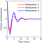
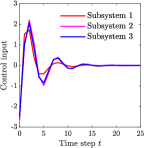
Figure 4: Responses of 33 with three subsystems $n=3$. The decentralized controller $\mathbf{u}_{i}=\mathbf{K}_{i}\mathbf{y}_{i}$, shown in 35, was computed via solving 34. (a) Output measurement $y_{i}[t]$; (b) Input $u_{i}[t]$.

We first consider an LTI system 33 with $n=3$ subsystems. For this small system, it took less than half a second to solve 34, resulting in the following decentralized controller

$$\mathbf{K}_{1} =\frac{-2.647z^{2}-0.04603z-0.02581}{z^{2}+0.01875z+0.009845},$$ (35)

$$\mathbf{K}_{2} =\frac{-2.515z^{2}+0.1379z-0.09867}{z^{2}-0.05334z+0.03937},$$

$$\mathbf{K}_{3} =\frac{-2.481z^{2}+0.1326z-0.06773}{z^{2}-0.05207z+0.02741}.$$

The order of each local controller $\mathbf{u}_{i}=\mathbf{K}_{i}\mathbf{y}_{i}$ is guaranteed to be the same with the state dimension of each subsystem (which is two in this case). Figure 4 shows the the responses of input $u_{i}[t]$ and output $y_{i}[t]$ when the initial state was $x_{i}[0]=\begin{bmatrix}0,\;1\end{bmatrix}^{{\mathsf{T}}},i=1,2,3$. As expected, the decentralized controller from 34 stabilizes the global system 33.

For comparison, we computed a centralized $\mathcal{H}_{2}$ optimal controller via SLP [13] according to [12, Section 7]. This SLP problem is infinite dimensional, and we used a standard FIR approximation for computation. Figure 5 (a) and (b) demonstrate the closed-loop responses using the resulting centralized dynamic controller when the FIR length was $10$ and $20$, respectively. Note that the FIR approximation always leads to a dynamical controller of high order (which scales linearly with respect to the FIR length): in particular, the order of the controller with FIR length $10$ is $84$ and the order of the controller with FIR length $20$ is $174$. In contrast, our LMI-based computation in Theorem 4 and Corollary 1 guarantees that the order of the resulting controller will be the same as the order of the system.

Moreover, it is known that the computational efficiency of the FIR approximation does not scale well with system dimension, as it leads to optimization problems of very large size. To illustrate this, we varied the number of subsystems from 6 to 14 in 33 and allow each subsystem to use its own state (i.e., $y_{i}[t]=x_{i}[t]$). Table I lists the time consumption for solving 34 and the SLP problem with FIR length $20$. It is clear that our LMI-based computation is much more scalable. For the case $n=14$, our LMI was two orders of magnitude faster to solve. Finally, as shown in Table II, the order of the dynamic controller 34 is always two whereas the order of the controller from the SLP increases dramatically, and is of order $1092$ when $n=14$, which is unpractical for deployment.

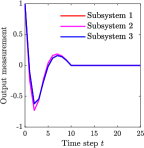
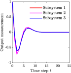
Figure 5: Responses of 33 with three subsystems $n=3$ under a centralized $\mathcal{H}_{2}$ optimal controller computed via SLP and FIR approximation. (Left) FIR length equals to $10$; (Right) FIR length equals to $20$.

Table I: Time (in seconds) for 34 and SLP + FIR (length 20). Includes YALMIP time and MOSEK time.

# of nodes $n$	6	8	10	12	14
LMI 34	0.49	0.60	0.75	0.99	1.28
SLP + FIR	3.22	8.60	22.68	53.19	132.87

Table II: Controller order for 34 and SLP + FIR (length 20).

# of nodes $n$	6	8	10	12	14
LMI 34	2	2	2	2	2
SLP + FIR	468	624	780	936	1092

VI Conclusions

In this paper, we have presented a kernel version of the Youla parameterization for stabilizing controllers $\mathcal{C}_{\mathrm{stab}}$. This parameterization only involves a single affine constraint, which can be viewed as a novel robust filtering problem. This filtering perspective leads to the first efficient LMI characterization for the frequency-domain characterization of $\mathcal{C}_{\mathrm{stab}}$. Our LMI characterization offers significant advantages compared to the existing parameterizations (SLP [13], IOP [6], and the mixed versions [12]) in terms of both computation and implementation. Ongoing research directions include investigations on LMIs for performance specifications under our new controller parameterization.

Appendix

VI-A State-space realization of the coprime factorization

It is straightforward to find a doubly coprime factorization for $\mathbf{G}(z)$ given a stabilizable and detectable state-space realization [1, Theorem 5.9]. This amounts to find a stabilizing feedback gain and observer gain.

Theorem 5

Suppose $\mathbf{G}(s)$ is a proper real-rational matrix and $\mathbf{G}=\left[\begin{array}[]{c|c}A&B\\ \hline\cr C&D\end{array}\right]$ is a stabilizable and detectable state-space realization. Let $F$ and $L$ be such that $A+BF$ and $A+LC$ are both stable. Then, a doubly co-prime factorization of $\mathbf{G}$ is

$$\begin{bmatrix}\mathbf{M}_{r}&\mathbf{V}_{r}\\ \mathbf{N}_{r}&\mathbf{U}_{r}\end{bmatrix}=\left[\begin{array}[]{c|cc}A+BF&B&L\\ \hline\cr F&I&0\\ C+DF&D&I\end{array}\right],\quad\begin{bmatrix}\mathbf{U}_{l}&-\mathbf{V}_{l}\\ -\mathbf{N}_{l}&\mathbf{M}_{l}\end{bmatrix}=\left[\begin{array}[]{c|cc}A+LC&-(B+LD)&L\\ \hline\cr F&I&0\\ C&-D&I\end{array}\right].$$ (36)

We can directly verify that the choices in 36 satisfy Definition 2 (see [22] for detailed computations). The coprime factorization of a transfer matrix in 36 has a feedback control interpretation [1, Remark 5.3]. For example, the right coprime factorization comes out naturally from changing the control variable by a state feedback.

Consider the state-space model

$$x[t+1] =Ax[t]+Bu[t],$$

$$y[t] =Cx[t]+Du[t].$$

Introduce a state feedback and change the variable $v[t]:=u[t]-Fx[t]$ where $F$ makes $A+BF$ stable. We then get

$$x[t+1] =(A+BF)x[t]+Bv[t],$$

$$u[t] =Fx[t]+v[t]$$

$$y[t] =(C+DF)x[t]+Dv[t].$$

From these equations, it is easy to see that the transfer matrix from $\mathbf{v}$ to $\mathbf{u}$ is

$$\mathbf{M}_{r}(z)=\left[\begin{array}[]{c|c}A+BF&B\\ \hline\cr F&I\end{array}\right],$$

and that the transfer matrix from $\mathbf{v}$ to $\mathbf{y}$ is

$$\mathbf{N}_{r}(z)=\left[\begin{array}[]{c|c}A+BF&B\\ \hline\cr C+DF&D\end{array}\right].$$

Therefore, we have $\mathbf{u}=\mathbf{M}_{r}\mathbf{v},\,\mathbf{y}=\mathbf{N}_{r}\mathbf{v},$ so that $\mathbf{y}=\mathbf{N}_{r}\mathbf{M}_{r}^{-1}\mathbf{u}$, i.e., $\mathbf{G}=\mathbf{N}_{r}\mathbf{M}_{r}^{-1}$.

VI-B Computation of 23

Here, we provide some detailed computation for 23. For notational convenience, we highlight ${\color[rgb]{0,0,1}\hat{A}},{\color[rgb]{0,0,1}\hat{B}},{\color[rgb]{0,0,1}\hat{C}},{\color[rgb]{0,0,1}\hat{D}}$ in blue.

• For 23a, we can verify

  $$\begin{bmatrix}I&0\\ 0&-V^{{\mathsf{T}}}N\end{bmatrix}^{{\mathsf{T}}}\begin{bmatrix}X&U\\ U^{{\mathsf{T}}}&\hat{X}\end{bmatrix}\begin{bmatrix}I&0\\ 0&-V^{{\mathsf{T}}}N\end{bmatrix}=\begin{bmatrix}I&0\\ 0&-NV\end{bmatrix}\begin{bmatrix}X&-UV^{{\mathsf{T}}}N\\ U^{{\mathsf{T}}}&-\hat{X}V^{{\mathsf{T}}}N\end{bmatrix}=\begin{bmatrix}X&-UV^{{\mathsf{T}}}N\\ -NVU^{{\mathsf{T}}}&NV\hat{X}V^{{\mathsf{T}}}N\end{bmatrix}$$

  Since $\tilde{P}\tilde{P}^{-1}=I$, we have

  $$U^{{\mathsf{T}}}Y+\hat{X}V^{{\mathsf{T}}}=0\quad\Rightarrow\quad-U^{{\mathsf{T}}}=\hat{X}V^{{\mathsf{T}}}N.$$ (37)

  Combining $Z=-UV^{{\mathsf{T}}}N$ with the two equations above leads to 23a.

• For 23b, we have

  $$\tilde{T}^{{\mathsf{T}}}\tilde{A}\tilde{P}\tilde{T} =\begin{bmatrix}I&0\\ 0&-V^{{\mathsf{T}}}N\end{bmatrix}^{{\mathsf{T}}}\begin{bmatrix}A&B_{1}{\color[rgb]{0,0,1}\hat{C}}\\ 0&{\color[rgb]{0,0,1}\hat{A}}\end{bmatrix}\begin{bmatrix}X&-UV^{{\mathsf{T}}}N\\ U^{{\mathsf{T}}}&-\hat{X}V^{{\mathsf{T}}}N\end{bmatrix}$$ (38)

  $$=\begin{bmatrix}A&B_{1}{\color[rgb]{0,0,1}\hat{C}}\\ 0&-NV{\color[rgb]{0,0,1}\hat{A}}\end{bmatrix}\begin{bmatrix}X&-UV^{{\mathsf{T}}}N\\ U^{{\mathsf{T}}}&-\hat{X}V^{{\mathsf{T}}}N\end{bmatrix}$$

  $$=\begin{bmatrix}AX+B_{1}{\color[rgb]{0,0,1}\hat{C}}U^{{\mathsf{T}}}&-AUV^{{\mathsf{T}}}N-B_{1}{\color[rgb]{0,0,1}\hat{C}}\hat{X}V^{{\mathsf{T}}}N\\ -NV{\color[rgb]{0,0,1}\hat{A}}U^{{\mathsf{T}}}&NV{\color[rgb]{0,0,1}\hat{A}}\hat{X}V^{{\mathsf{T}}}N\end{bmatrix}.$$

  Considering 37, we have $NV{\color[rgb]{0,0,1}\hat{A}}\hat{X}V^{{\mathsf{T}}}N=-NV{\color[rgb]{0,0,1}\hat{A}}U^{{\mathsf{T}}}$. Also, the change of variables in 22 reads as

  $$\begin{bmatrix}Q&F\\ L&R\end{bmatrix}:=\begin{bmatrix}-NV{\color[rgb]{0,0,1}\hat{A}}U^{{\mathsf{T}}}&-NV{\color[rgb]{0,0,1}\hat{B}}\\ {\color[rgb]{0,0,1}\hat{C}}U^{{\mathsf{T}}}&{\color[rgb]{0,0,1}\hat{D}}\end{bmatrix},$$

  Combining 22, 37 with 38 leads to 23b.

• For 23c, we have

  $$\begin{bmatrix}I&0\\ 0&-V^{{\mathsf{T}}}N\end{bmatrix}^{{\mathsf{T}}}\begin{bmatrix}B_{1}{\color[rgb]{0,0,1}\hat{D}}-B_{2}\\ {\color[rgb]{0,0,1}\hat{B}}\end{bmatrix}=\begin{bmatrix}I&0\\ 0&-NV\end{bmatrix}\begin{bmatrix}B_{1}{\color[rgb]{0,0,1}\hat{D}}-B_{2}\\ -NV{\color[rgb]{0,0,1}\hat{B}}\end{bmatrix}.$$

• For 23d, we have

  $$\tilde{C}\tilde{P}\tilde{T}=\begin{bmatrix}C&D_{1}{\color[rgb]{0,0,1}\hat{C}}\end{bmatrix}\begin{bmatrix}X&-UV^{{\mathsf{T}}}N\\ U^{{\mathsf{T}}}&-\hat{X}V^{{\mathsf{T}}}N\end{bmatrix}=\begin{bmatrix}CX+D_{1}{\color[rgb]{0,0,1}\hat{C}}U^{{\mathsf{T}}}&-CUV^{{\mathsf{T}}}N-D_{1}{\color[rgb]{0,0,1}\hat{C}}\hat{X}V^{{\mathsf{T}}}N\end{bmatrix}$$

  Combining $Z=-UV^{{\mathsf{T}}}N$ and 37 with the equation above leads to 23d.

VI-C Proof of Corollary 1

The first part of Corollary 1 is immediate. Given $\mathbf{X}$ and $\mathbf{Y}$ in 30, we prove the following state space realization

$$\mathbf{K}=\mathbf{Y}\mathbf{X}^{-1}=\left[\begin{array}[]{c|c}\hat{A}-\hat{B}\hat{D}_{X}^{-1}\hat{C}_{X}&-\hat{B}\hat{D}_{X}^{-1}\\ \hline\cr-\hat{C}_{Y}+\hat{D}_{Y}\hat{D}_{X}^{-1}\hat{C}_{X}&\hat{D}_{Y}\hat{D}_{X}^{-1}\end{array}\right].$$ (39)

The proof is based on a few standard system operations. We recall some of them below (see [1, Chapter 3.6] for more discussions). Consider two dynamical systems

$$\mathbf{G}_{i}=\left[\begin{array}[]{c|c}A_{i}&B_{i}\\ \hline\cr C_{i}&D_{i}\end{array}\right],\quad i=1,2.$$

Their inverses are given by

$$\mathbf{G}_{i}^{-1}=\left[\begin{array}[]{c|c}A_{i}-B_{i}D_{i}^{-1}C_{i}&-B_{i}D_{i}^{-1}\\ \hline\cr D_{i}^{-1}C_{i}&D_{i}^{-1}\end{array}\right],i=1,2$$

where we assume $D_{i}$ is invertible. The cascade connection of two systems such that $\mathbf{y}=\mathbf{G}_{1}\mathbf{G}_{2}\mathbf{u}$ has a state-space realization

$$\mathbf{G}_{1}\mathbf{G}_{2}=\left[\begin{array}[]{c c|c}A_{1}&B_{1}C_{2}&B_{1}D_{2}\\ 0&A_{2}&B_{2}\\ \hline\cr C_{1}&D_{1}C_{2}&D_{1}D_{2}\end{array}\right].$$ (40)

Note that 40 is in general not minimal (there may be uncontrollable and observable modes). For example, when $\mathbf{G}_{1}=\mathbf{G}_{2}^{-1}$, we have $\mathbf{G}_{1}\mathbf{G}_{2}=I$. For any invertible matrix $T$ with compatible dimension, we have

$$\mathbf{G}_{i}=\left[\begin{array}[]{c|c}A_{i}&B_{i}\\ \hline\cr C_{i}&D_{i}\end{array}\right]=\left[\begin{array}[]{c|c}TA_{i}T^{-1}&TB_{i}\\ \hline\cr C_{i}T^{-1}&D_{i}\end{array}\right],i=1,2.$$ (41)

Now, consider the state-space realization of $\mathbf{X}$ and $\mathbf{Y}$ in 30, we have

$$\mathbf{X}^{-1}=\left[\begin{array}[]{c|c}\hat{A}-\hat{B}\hat{D}_{X}^{-1}\hat{C}_{X}&-\hat{B}\hat{D}_{X}^{-1}\\ \hline\cr\hat{D}_{X}^{-1}\hat{C}_{X}&\hat{D}_{X}^{-1}\end{array}\right],$$

and

$$\mathbf{Y}\mathbf{X}^{-1} =\left[\begin{array}[]{c|c}\hat{A}&\hat{B}\\ \hline\cr\hat{C}_{Y}&\hat{D}_{Y}\end{array}\right]\left[\begin{array}[]{c|c}\hat{A}-\hat{B}\hat{D}_{X}^{-1}\hat{C}_{X}&-\hat{B}\hat{D}_{X}^{-1}\\ \hline\cr\hat{D}_{X}^{-1}\hat{C}_{X}&\hat{D}_{X}^{-1}\end{array}\right]$$

$$=\left[\begin{array}[]{c c|c}\hat{A}&\hat{B}\hat{D}_{X}^{-1}\hat{C}_{X}&\hat{B}\hat{D}_{X}^{-1}\\ 0&\hat{A}-\hat{B}\hat{D}_{X}^{-1}\hat{C}_{X}&-\hat{B}\hat{D}_{X}^{-1}\\ \hline\cr\hat{C}_{Y}&\hat{D}_{Y}\hat{D}_{X}^{-1}\hat{C}_{X}&\hat{D}_{Y}\hat{D}_{X}^{-1}\end{array}\right].$$

From 41, upon defining a transformation

$$T=\begin{bmatrix}I&I\\ 0&I\end{bmatrix},\qquad T^{-1}=\begin{bmatrix}I&-I\\ 0&I\end{bmatrix}$$

with compatible dimension, we have

$$\mathbf{Y}\mathbf{X}^{-1}=\left[\begin{array}[]{c c|c}\hat{A}&0&0\\ 0&\hat{A}-\hat{B}\hat{D}_{X}^{-1}\hat{C}_{X}&-\hat{B}\hat{D}_{X}^{-1}\\ \hline\cr\hat{C}_{Y}&\hat{D}_{Y}\hat{D}_{X}^{-1}\hat{C}_{X}-\hat{C}_{Y}&\hat{D}_{Y}\hat{D}_{X}^{-1}\end{array}\right]=\left[\begin{array}[]{c|c}\hat{A}-\hat{B}\hat{D}_{X}^{-1}\hat{C}_{X}&-\hat{B}\hat{D}_{X}^{-1}\\ \hline\cr-\hat{C}_{Y}+\hat{D}_{Y}\hat{D}_{X}^{-1}\hat{C}_{X}&\hat{D}_{Y}\hat{D}_{X}^{-1}\end{array}\right].$$

This completes the proof of 39.

VI-D Extended LMI formulation

We use another $\mathcal{H}_{\infty}$ lemma from [23] to derive a new LMI for solving the right robust filtering problem.

Lemma 5 (​​[23])

Given a stable transfer function $\mathbf{G}(z)=C(zI-A)^{-1}B+D\in\mathcal{RH}_{\infty}$, then $\|\mathbf{G}(z)\|^{2}_{\infty}<\mu$ if and only if there exist a positive definite matrix $P$ and a matrix $G$ such that

$$\begin{bmatrix}P&AG&B&0\\ GA^{{\mathsf{T}}}&G+G^{{\mathsf{T}}}-P&0&GC^{{\mathsf{T}}}\\ B^{{\mathsf{T}}}&0&I&D^{{\mathsf{T}}}\\ 0&CG&D&\mu I\end{bmatrix}\succ 0.$$ (42)

We refer the interested reader to [23] for discussions on the features of this extended LMI 42 compared to the standard LMI 17. Using this extended $\mathcal{H}_{\infty}$ lemma, we can derive anther LMI to solve the right $\mathcal{H}_{\infty}$ filtering problem (15).

Theorem 6

There exists $\mathbf{F}(z)\in\mathcal{RH}_{\infty}$ such that (15) holds if and only if there exist symmetric matrices $E,H$, and matrices $X,Z,N,G$, and $Q,F,L,R$ such that

$$\begin{bmatrix}E&G&AX+B_{1}L&A(X-N)+B_{1}L&B_{1}R-B_{2}&0\\ \star&H&Q&Q&F&0\\ \star&\star&X+X^{{\mathsf{T}}}-E&X-N+Z^{{\mathsf{T}}}-G&0&X^{{\mathsf{T}}}C^{{\mathsf{T}}}+L^{{\mathsf{T}}}D_{1}^{{\mathsf{T}}}\\ \star&\star&\star&Z+Z^{{\mathsf{T}}}-H&0&(X-N)^{{\mathsf{T}}}C^{{\mathsf{T}}}+L^{{\mathsf{T}}}D_{1}^{{\mathsf{T}}}\\ \star&\star&\star&\star&I&R^{{\mathsf{T}}}D_{1}^{{\mathsf{T}}}-D_{2}^{{\mathsf{T}}}\\ \star&\star&\star&\star&\star&\mu_{1}I\end{bmatrix}\succ 0.$$ (43)

where $\star$ denotes the symmetric counterparts. If (43) holds, a state-space realization of $F(z)=\hat{C}(zI-\hat{A})\hat{B}+\hat{D}$ is

$$\begin{bmatrix}\hat{A}&\hat{B}\\ \hat{C}&\hat{D}\end{bmatrix}=\begin{bmatrix}UZ^{-1}&0\\ 0&I\end{bmatrix}\begin{bmatrix}Q&F\\ L&R\end{bmatrix}\begin{bmatrix}U^{-1}&0\\ 0&I\end{bmatrix},$$ (44)

where $U$ is an arbitrary non-singular matrix.

References

- [1] K. Zhou, J. C. Doyle, K. Glover et al., Robust and optimal control. Prentice hall New Jersey, 1996, vol. 40.
- [2] S. P. Boyd and C. H. Barratt, Linear controller design: limits of performance. Prentice Hall Englewood Cliffs, NJ, 1991.
- [3] A. Francis, A course in control theory. Springer-Verlag, 1987.
- [4] D. Youla, H. Jabr, and J. Bongiorno, “Modern Wiener-Hopf design of optimal controllers–Part II: The multivariable case,” IEEE Trans. Autom. Control., vol. 21, no. 3, pp. 319–338, 1976.
- [5] J. Anderson, J. C. Doyle, S. H. Low, and N. Matni, “System level synthesis,” Annual Reviews in Control, 2019.
- [6] L. Furieri, Y. Zheng, A. Papachristodoulou, and M. Kamgarpour, “An input-output parametrization of stabilizing controllers: amidst Youla and system level synthesis,” IEEE Control Systems Letters, vol. 3, no. 4, pp. 1014–1019, Oct 2019.
- [7] Y. Zheng, L. Furieri, M. Kamgarpour, and N. Li, “Sample complexity of linear quadratic gaussian (lqg) control for output feedback systems,” in Learning for Dynamics and Control. PMLR, 2021, pp. 559–570.
- [8] S. Dean, H. Mania, N. Matni, B. Recht, and S. Tu, “On the sample complexity of the linear quadratic regulator,” Foundations of Computational Mathematics, vol. 20, no. 4, pp. 633–679, 2020.
- [9] Y. Zhang, S. K. Ukil, E. Neimand, S. Sabau, and M. E. Hohil, “Sample complexity of the robust LQG regulator with coprime factors uncertainty,” arXiv preprint arXiv:2109.14164, 2021.
- [10] Y. Zheng, L. Furieri, A. Papachristodoulou, N. Li, and M. Kamgarpour, “On the equivalence of youla, system-level, and input–output parameterizations,” IEEE Transactions on Automatic Control, vol. 66, no. 1, pp. 413–420, 2020.
- [11] S.-H. Tseng, “Realization-stability lemma for controller synthesis,” arXiv preprint arXiv:2112.02005, 2021.
- [12] Y. Zheng, L. Furieri, M. Kamgarpour, and N. Li, “System-level, input–output and new parameterizations of stabilizing controllers, and their numerical computation,” Automatica, vol. 140, p. 110211, 2022.
- [13] Y.-S. Wang, N. Matni, and J. C. Doyle, “A system level approach to controller synthesis,” IEEE Trans. Autom. Control., 2019.
- [14] L. Furieri, Y. Zheng, A. Papachristodoulou, and M. Kamgarpour, “Sparsity invariance for convex design of distributed controllers,” IEEE Trans. Control Netw. Syst., pp. 1–12, 2020.
- [15] M. Rotkowitz and S. Lall, “A characterization of convex problems in decentralized control,” IEEE transactions on Automatic Control, vol. 50, no. 12, pp. 1984–1996, 2005.
- [16] J. C. Geromel, J. Bernussou, G. Garcia, and M. C. de Oliveira, “ and robust filtering for discrete-time linear systems,” SIAM Journal on Control and Optimization, vol. 38, pp. 1353–1368, 2000.
- [17] J. C. Geromel, M. C. de Oliveira, and J. Bernussou, “Robust filtering of discrete-time linear systems with parameter dependent lyapunov functions,” SIAM Journal on control and optimization, vol. 41, no. 3, pp. 700–711, 2002.
- [18] G. E. Dullerud and F. Paganini, A course in robust control theory: a convex approach. Springer Science & Business Media, 2013, vol. 36.
- [19] P. Gahinet and P. Apkarian, “A linear matrix inequality approach to control,” International Journal of Robust and Nonlinear Control, vol. 4, no. 4, pp. 421–448, 1994.
- [20] C. Scherer, P. Gahinet, and M. Chilali, “Multiobjective output-feedback control via LMI optimization,” IEEE Transactions on Automatic Control, vol. 42, no. 7, pp. 896–911, 1997.
- [21] Y. Zheng, Y. Tang, and N. Li, “Analysis of the optimization landscape of Linear Quadratic Gaussian (LQG) control,” arXiv preprint arXiv:2102.04393, 2021.
- [22] C. Nett, C. Jacobson, and M. Balas, “A connection between state-space and doubly coprime fractional representations,” IEEE Trans. Autom. Control., vol. 29, no. 9, pp. 831–832, 1984.
- [23] M. C. De Oliveira, J. C. Geromel, and J. Bernussou, “Extended and norm characterizations and controller parametrizations for discrete-time systems,” International Journal of Control, vol. 75, no. 9, pp. 666–679, 2002.
- [24] L. Bakule, “Decentralized control: An overview,” Annual reviews in control, vol. 32, no. 1, pp. 87–98, 2008.
- [25] J. Löfberg, “Yalmip: A toolbox for modeling and optimization in matlab,” in Proceedings of the CACSD Conference, vol. 3. Taipei, Taiwan, 2004.
- [26] E. D. Andersen and K. D. Andersen, “The MOSEK interior point optimizer for linear programming: an implementation of the homogeneous algorithm,” in High performance optimization. Springer, 2000.
- [27] Y. Zheng, R. P. Mason, and A. Papachristodoulou, “Scalable design of structured controllers using chordal decomposition,” IEEE Transactions on Automatic Control, vol. 63, no. 3, pp. 752–767, 2017.