MBORE: Multi-objective Bayesian Optimisation by
Density-Ratio Estimation

Abstract.

Optimisation problems often have multiple conflicting objectives that can be computationally and/or financially expensive. Mono-surrogate Bayesian optimisation (BO) is a popular model-based approach for optimising such black-box functions. It combines objective values via scalarisation and builds a Gaussian process (GP) surrogate of the scalarised values. The location which maximises a cheap-to-query acquisition function is chosen as the next location to expensively evaluate. While BO is an effective strategy, the use of GPs is limiting. Their performance decreases as the problem input dimensionality increases, and their computational complexity scales cubically with the amount of data. To address these limitations, we extend previous work on BO by density-ratio estimation (BORE) to the multi-objective setting. BORE links the computation of the probability of improvement acquisition function to that of probabilistic classification. This enables the use of state-of-the-art classifiers in a BO-like framework. In this work we present MBORE: multi-objective Bayesian optimisation by density-ratio estimation, and compare it to BO across a range of synthetic and real-world benchmarks. We find that MBORE performs as well as or better than BO on a wide variety of problems, and that it outperforms BO on high-dimensional and real-world problems.

1. Introduction

Optimisation problems, particularly those in real-world settings, often have conflicting objectives that can be computationally and/or financially expensive to evaluate. For example, it is often desirable to maximise a robot’s speed and minimise its energy consumption (Liao et al., 2019), or to maximise crop yield while minimising the environmental impacts the required agricultural development (Jiang et al., 2020). These tend to be black-box problems, i.e. they have no closed-form or derivative information available. In order to optimise these expensive black-box functions, a common strategy is to create surrogate models for each of the objective functions and perform optimisation on these instead, choosing where to evaluate the expensive functions next based on locations that are predicted to yield high-quality solutions.

A plethora of multi-objective surrogate-based approaches have been proposed in recent years (Rahat et al., 2017; Chugh et al., 2018; Belakaria et al., 2019; Yang et al., 2019; Suzuki et al., 2020; Tiao et al., 2021). These are usually inspired by, or directly use, the framework of single-objective Bayesian optimisation (BO). In BO, given an initial set of expensively evaluated solutions, a surrogate model, often a probabilistic model such as a Gaussian process (GP), is created for either each objective function (a multi-surrogate approach), or a scalarised representation of the multiple objectives (a mono-surrogate approach). In these approaches, an acquisition function, also known as an infill criterion, is optimised to suggest the next location to expensively evaluate. These attempt to balance the exploration of locations with high amounts of prediction uncertainty with the exploitation of locations that have good predicted values. They are also cheap-to-query and, therefore, transform the expensive optimisation problem into a sequence of cheaper ones followed by an expensive evaluation. Once a new candidate solution has been selected and evaluated, the surrogate models are retrained with the new solution and the process is repeated ad libitum.

Mono-surrogate approaches are known to be considerably faster than multi-surrogate approaches (Chugh, 2020). Using only one surrogate model offers large computational savings because the model of choice, GPs, scale cubically in the number of solutions the model is trained on (Rasmussen and Williams, 2006), leading to large amounts of computation needed for larger numbers of solutions. Acquisition functions that have been designed for BO (e.g. Jones et al., 1998; Srinivas et al., 2010; Wang and Jegelka, 2017; De Ath et al., 2021), can be used without alteration. Single-objective acquisition functions are usually cheap to evaluate, unlike those used in multi-surrogate approaches. These often need to carry out expensive multidimensional integrations, such as when calculating the expected hypervolume improvement criterion (Emmerich, 2005).

Despite the success of mono-surrogate approaches, they are not without limitations. The aforementioned cubic scaling of GPs leads to model training times increasing as the number of solutions grows. Similarly, GPs are known to suffer greatly from the curse of dimensionality. Specifically, the modelling ability of nonparametric regression depends exponentially on the problem dimensionality (Györfi et al., 2002). Approaches to address these fundamental problems with GPs usually involve either reducing the number solutions included in the GP models via inducing point methods (Snelson and Ghahramani, 2006; Titsias, 2009; Wilson and Nickisch, 2015; Salimbeni et al., 2018; Shi et al., 2020), or making assumptions about the underlying structure of the function of interest to simplify the inference, such as assuming that it resides on a low-dimensional manifold (Wang et al., 2013; Kandasamy et al., 2015; Wang et al., 2017; Gardner et al., 2017; Rolland et al., 2018; Letham et al., 2020). However, these necessarily lead to poorer modelling of target function (Letham et al., 2020).

An alternative approach to improving the modelling in BO is to use a different surrogate model, such as a random forest (Hutter et al., 2011) or neural network (Snoek et al., 2015). However, these models do not usually come with principled ways to compute prediction uncertainty, limiting their applicability to Bayesian optimisation. Recently, Tiao et al. (2021) proposed to carry out BO via density-ratio estimation (BORE), a generalisation of the classical tree-structured Parzen estimator (Bergstra et al., 2011). They claimed that maximising the expected improvement over the best-seen function value in a probabilistic regression model, the most popular formulation of BO, is equivalent to maximising the class-posterior probability of classifier trained with a proper scoring rule (Gneiting and Raftery, 2007). Unfortunately, this claim is only partially correct (Song and Ermon, 2021). Garnett (2022) demonstrates that, in fact, maximising the class-posterior probability is equivalent to maximising the probability of improvement. Nevertheless, the result is important because it still facilitates the use of most state-of-the-art classifiers, such as neural networks or gradient boosted trees (Chen and Guestrin, 2016). Naturally, this leads to a vast reduction in computational complexity as well as an increase in modelling capability of surrogate models available for use in BO. Therefore, this allows for higher-dimensional problems to be tackled by using more suitable models, e.g. neural networks, which are well-known for having universal function approximation guarantees (Hornik et al., 1989).

In this work, we extend BORE to the multi-objective setting via the use of scalarising functions (Hwang and Masud, 1979; Chugh, 2020), a mono-surrogate approach. Specifically, we compare MBORE, our proposed multi-objective version of BORE, using two different classification models: a fully-connected neural network and gradient boosted machines (XGBoost (Chen and Guestrin, 2016)) with the standard BO approach using a GP. We compare their performance when using three existing scalarisation approaches, augmented Tchebycheff (Knowles, 2006), hypervolume improvement (Rahat et al., 2017) and dominance ranking (Rahat et al., 2017), as well as Pareto hypervolume contribution (PHC), a novel scalarisation method proposed in this work. Multi-objective BO and MBORE are evaluated on two synthetic benchmark suites, DTLZ (Deb et al., 2005) and WFG (Huband et al., 2006), across a range of problem dimensionalities and numbers of objectives, as well as a recently proposed real-world set of benchmark problems (Tanabe and Ishibuchi, 2020). Additionally, we also investigate the performance of BO and MBORE on high-dimensional problems using the WFG benchmark, and empirically compare their computational costs.

Our main contributions can be summarised as follows:

1. We present MBORE, a novel mono-surrogate multi-objective classification-based BO approach using scalarisation.

2. We also present PHC, a new scalariser that directly uses the hypervolume contribution of a solution to its Pareto shell.

3. We compare MBORE and BO, using two probabilistic classifiers and several popular scalarisation methods, across a range of synthetic and real-world test problems.

4. Empirically, we show that MBORE is equal to or better than BO on a wide range of problems, particularly when using PHC, and that MBORE is considerably better than BO on the evaluated real-world and high-dimensional problems, all while using a fraction of the computational resources.

We begin in Section 2 by providing an overview of both single- and multi-objective BO, including a review of GPs, acquisition functions and scalarisation methods. Section 3 introduces BO by density-ratio estimation and, in Section 4, we extend it to the multi-objective setting. An extensive experimental evaluation of BO and MBORE is carried out in Section 5, along with a discussion of the results. We finish with concluding remarks in Section 6.

2. Bayesian Optimisation Framework

In this section we first describe single-objective Bayesian optimisation, including its two main components, the Gaussian process surrogate model and acquisition function. We then go on to show how BO can be extended to the multi-objective setting via scalarisation, giving examples of the scalarisation methods used in this work, along with the proposal of a new scalariser.

2.1. Bayesian Optimisation

Bayesian optimisation (BO) was first proposed for single-objective problems by Kushner (1964), and later improved by Močkus et al. (1978) and Jones et al. (1998). Interested readers should refer to (Shahriari et al., 2016) and (Frazier, 2018) for recent and comprehensive surveys on the topic. BO is a global search strategy that sequentially samples design space at locations that are likely to contain the global optimum, while taking into account the prediction of a surrogate model and its associated uncertainty (Jones et al., 1998). The single-objective optimisation problem can be defined as finding a minimum of an unknown objective function $f:\mathcal{X}\mapsto\mathbb{R}$, defined on a compact domain $\mathcal{X}\subset\mathbb{R}^{d}$:

(1) $$\min_{\mathbf{x}\in\mathcal{X}}f(\mathbf{x}).$$

BO starts by using a space-filling algorithm, such as Latin hypercube sampling (McKay et al., 1979), to generate an initial set of solutions $\{\mathbf{x}_{i}\}_{i=1}^{t}$, and then expensively evaluates them with the objective function. These observations form the dataset $\mathcal{D}=\{(\mathbf{x}_{i},f_{i}\triangleq f(\mathbf{x}_{i}))\}_{i=1}^{t}$ that the initial surrogate model is trained with. Following model training, and at each subsequent iteration, the next location to expensively evaluate is chosen as the location $\mathbf{x}^{\prime}$ that maximises an acquisition function $\alpha(\mathbf{x})$, i.e. $\mathbf{x}^{\prime}=\operatorname*{\arg\!\max}_{\mathbf{x}\in\mathcal{X}}\alpha(\mathbf{x})$. The dataset is then augmented with $\{\mathbf{x}^{\prime},f(\mathbf{x}^{\prime})\}$ and the process is repeated until budget exhaustion. The global minimum of $f$ is then estimated to be the best-observed value thus far, $f^{\star}=\min\{f_{i}\}$.

2.1.1. Gaussian Processes

Gaussian processes (GP) are a common choice of surrogate model due to their strengths in uncertainty quantification and function approximation (Rasmussen and Williams, 2006). They define a prior distribution over functions, such that any finite number of drawn function values are jointly Gaussian, with mean $m(\mathbf{x})$ and covariance $\kappa(\mathbf{x},\mathbf{x}^{\prime}\,|\,\boldsymbol{\theta})$, with hyperparameters $\boldsymbol{\theta}$. Without loss of generality, we use a zero-mean prior $m(\mathbf{x})=0\,\forall\,\mathbf{x}\in\mathcal{X}$; see (De Ath et al., 2020) for alternatives. Conditioning the GP prior distribution on data consisting of $t$ sampled locations $\mathcal{D}=\{(\mathbf{x}_{i},f_{i}\triangleq f(\mathbf{x}_{i}))\}_{i=1}^{t}$ leads to a posterior distribution that is also a GP:

(2) $$p(f(\mathbf{x})\,|\,\mathbf{x},\mathcal{D},\boldsymbol{\theta})=\mathcal{N}(\mu(\mathbf{x}),\sigma^{2}(\mathbf{x}))$$

with mean and variance

(3) $$\mu(\mathbf{x}\,|\,\mathcal{D},\boldsymbol{\theta}) =\boldsymbol{\kappa}(\mathbf{x},\mathbf{X})\mathbf{K}^{-1}\mathbf{y}$$

(4) $$\sigma^{2}(\mathbf{x}\,|\,\mathcal{D},\boldsymbol{\theta}) =\kappa(\mathbf{x},\mathbf{x})-\boldsymbol{\kappa}(\mathbf{x},\mathbf{X})^{\top}\mathbf{K}^{-1}\boldsymbol{\kappa}(\mathbf{X},\mathbf{x}).$$

Here, $\mathbf{X}\in\mathbb{R}^{t\times d}$ is a matrix of input locations in each row and $\mathbf{y}=(f_{1},f_{2},\dots,f_{t})^{\top}$ is the corresponding vector of expensive function evaluations. The kernel matrix $\mathbf{K}\in\mathbb{R}^{t\times t}$ is $\mathbf{K}_{ij}=\kappa(\mathbf{x}_{i},\mathbf{x}_{j}\,|\,\boldsymbol{\theta})$ and $\boldsymbol{\kappa}(\mathbf{x},\mathbf{X})\in\mathbb{R}^{t}$ is given by $[\boldsymbol{\kappa}(\mathbf{x},\mathbf{X})]_{i}=\kappa(\mathbf{x},\mathbf{x}_{i}\,|\,\boldsymbol{\theta})$. In this work we use a Matérn $5/2$ kernel, as recommended for modelling realistic functions (Stein, 1999; Snoek et al., 2012). The kernel’s hyperparameters $\boldsymbol{\theta}$ are learnt via maximising the log marginal likelihood (Rasmussen and Williams, 2006; De Ath et al., 2021).

2.1.2. Acquisition Functions

Acquisition functions ${\alpha:\mathcal{X}\mapsto\mathbb{R}}$ measure the expected utility of expensively evaluating $f$ at any location $\mathbf{x}$. Its maximiser is chosen as the next location to expensively evaluate. This strategy allows for an estimate of the global optimum to be generated cheaply via the surrogate model, rather than by repeatedly querying the expensive objective function. The probability of improvement (PI) (Kushner, 1964) is one of the earliest infill criteria. It is the probability that the predicted value at a location $\mathbf{x}$ is less than a threshold $\tau$, which, if the posterior distribution is Gaussian, can be expressed in closed form as

(5) $$\alpha_{\textsc{pi}}(\mathbf{x},\tau)=p(f(\mathbf{x})<\tau\,|\,\mathcal{D},\boldsymbol{\theta})=\Phi(s).$$

Here, $\tau$ is usually set to the best solution seen thus far, $s=(\tau-\mu(\mathbf{x}))/\sigma(\mathbf{x})$ is the predicted improvement normalised by its uncertainty, and $\Phi(\cdot)$ is the standard Gaussian cumulative density function. Its successor, the expected improvement (EI) (Močkus et al., 1978; Jones et al., 1998), is one of the most common acquisition functions and measures the expected positive predicted improvement over a threshold $\tau$. It is expressible in closed-form under the same assumptions (Jones et al., 1998):

(6) $$\alpha_{\textsc{ei}}(\mathbf{x},\tau)=\sigma(\mathbf{x})\left[s\Phi\left(s\right)+\phi\left(s\right)\right],$$

where $\phi(\cdot)$ is the standard Gaussian probability density function.

In practice, EI is often preferred because PI tends to be overly-exploitative (Jones et al., 1998; De Ath et al., 2021). However, many other acquisition functions have been proposed, including optimistic strategies such as upper confidence bound (Srinivas et al., 2010), information-theoretic approaches (Scott et al., 2011; Hennig and Schuler, 2012; Henrández-Lobato et al., 2014; Wang and Jegelka, 2017; Ru et al., 2018), and $\epsilon$-greedy strategies (Bull, 2011; De Ath et al., 2021).

2.2. Multi-objective Bayesian Optimisation

Real-world optimisation problems often have multiple conflicting objectives, all of which must be minimised at the same time (Coello et al., 2006). The multi-objective optimisation problem can be defined as simultaneously minimising $M\geq 2$ unknown objective functions

(7) $$\min_{\mathbf{x}\in\mathcal{X}}\mathbf{F}(\mathbf{x})=(f^{1}(\mathbf{x}),\dots,f^{M}(\mathbf{x})),$$

where $f^{i}$ is the $i$-th objective value and $\mathbf{F}:\mathcal{X}\mapsto\mathbb{R}^{M}$. Assuming that problem contains conflicting objectives, then there will not be a one unique solution. Instead, possibly infinitely many solutions may exist that trade off between the different objectives. The trade-off between solutions is often characterised by a dominance relationship: $\mathbf{x}$ is said to dominate $\mathbf{x}^{\prime}$, denoted $\mathbf{x}\prec\mathbf{x}^{\prime}$, iff:

(8) $$\forall i\in\{1,2,\dots M\}\left(f^{i}(\mathbf{x})\leq f^{i}(\mathbf{x}^{\prime})\right)\wedge\exists i\,\left(f^{i}(\mathbf{x})<f^{i}(\mathbf{x}^{\prime})\right).$$

The set containing solutions that optimally trades off between the objectives is referred to as the Pareto set:

(9) $$\mathcal{P}=\{\mathbf{x}\,|\,\mathbf{x}^{\prime}\!\not\prec\mathbf{x}\,\wedge\,\mathbf{x},\mathbf{x}^{\prime}\in\mathcal{X}\},$$

where $\mathbf{x}^{\prime}\!\not\prec\mathbf{x}$ indicates that $\mathbf{x}^{\prime}$ does not dominate $\mathbf{x}$. Computation of $\mathcal{P}$ is infeasible, due to its potentially infinite size. Thankfully, an approximation is often sufficient, leading to the goal of generating a good approximation $\tilde{\mathcal{P}}$ to the Pareto set $\mathcal{P}$.

Knowles (2006) presented the first mono-surrogate approach for multi-objective BO. They proposed to scalarise the objective function values $(f^{1},f^{2},\dots,f^{M})$, i.e. mapping them to a single value, via the use of a scalarising function. It uses the randomly-weighted normalised objective values in an augmented Tchebycheff function, drawing weightings from a set of predefined weights to scalarise the sets of objective values. These can then be used in lieu of the objective values, directly within the BO framework (Section 2.1). The location that maximises the expected improvement over the best-seen scalarisation is then chosen to be expensively evaluated.

2.2.1. Scalarisation functions

The augmented Tchebycheff scalarisation was the de facto choice for multi-objective BO. However, Rahat et al. (2017) recently proposed several scalarisation that outperform it. Subsequentially, Chugh (2020) conducted an exhaustive study of scalarisation methods for multi-objective BO, comparing those in (Rahat et al., 2017) to several outside the BO literature. They show that the choosing the best scalarisation method is far from trivial and is, in fact, problem dependent. It is also noted that the ease with which a GP may model a landscape produced by a scalarisation is problem dependent, i.e. the same scalarisation may produce easier or harder landscapes for a GP to model, relative to other methods.

The main properties required for a scalarisation to be used in the BO framework is that it should preserve dominance relationships and allow for every Pareto optimal solution to be reached (Hwang and Masud, 1979). In doing so, the maximisation of a dominance-preserving scalarisation should lead to an improvement in the Pareto set (Zitzler and Künzli, 2004). Although many methods have been proposed, we focus on the popular augmented Tchebycheff method (Knowles, 2006), two of the best-performing in (Rahat et al., 2017), and a novel scalarisation proposed in this work.

Augmented Tchebycheff (AT)

First presented for BO by Knowles (2006), the augmented Tchebycheff method combines the Tchebycheff function with a weighted sum, scaled by a small positive value $\rho$:

(10) $$g_{\textsc{at}}(\mathbf{x},X)=\max_{i}\left[w^{i}\bar{f}^{i}\right]+\rho\sum_{i=1}^{M}w^{i}\bar{f}^{i},$$

where $\bar{f}^{i}\in[0,1]$ are the normalised versions of the observed objective values. At each BO iteration, the weights $\mathbf{w}=(w^{1},w^{2},\dots,w^{M})$, where $|\mathbf{w}|=1$, are sampled uniformly from a fixed set of evenly distributed weight vectors on the $M$-dimensional unit simplex.

Hypervolume Improvement (HypI)

The hypervolume indicator $H(X,\mathbf{r})$ measures the volume of space dominated by a set of solutions $X=\{\mathbf{x}_{1},\mathbf{x}_{2},\dots,\mathbf{x}_{t}\}$ relative to a reference vector $\mathbf{r}$ (Zitzler, 1999). It is a popular choice for comparing two sets of solutions in because maximising it is equivalent to locating the optimal Pareto set (Fleischer, 2003). In order to turn the hypervolume indicator into a scalariser, it is natural to consider the contribution of each set member, i.e. the amount of hypervolume gained by including a set member. However, only solutions that reside within the Pareto set of $X$ will have a non-zero contribution, even if solutions dominated by the Pareto set dominate other solutions, they will all be assigned a value of zero. This would hinder the progress of BO because it would create a plateau that lacks spatial information about solution quality.

Rahat et al. (2017) proposed a solution to the inherent problems of solely using the hypervolume contribution that they named the hypervolume improvement (HYPI). The members of $X$ are first ranked according to Pareto shells in which they reside. Let the first Pareto shell $\mathcal{P}^{1}$ be the Pareto set of $X$, i.e. $\mathcal{P}^{1}=\textsc{nondom}(X)$, where $\textsc{nondom}(X)$ returns the non-dominated members of $X$. Subsequent Pareto shells $\mathcal{P}^{\lambda}$, with $(\lambda>1)$, can then be defined as

(11) $$\mathcal{P}^{\lambda}=\textsc{nondom}\left(X\setminus\bigcup_{i=1}^{\lambda-1}\mathcal{P}^{i}\right).$$

Once the members of $X$ have been ranked, the HYPI of a solution $\mathbf{x}$ is defined to be the hypervolume of the union of $\mathbf{x}$ and the first Pareto shell $\mathcal{P}^{\dagger}$ that contains no solutions that dominate it:

(12) $$g_{\textsc{hypi}}(\mathbf{x},X)=H\left(\{\mathbf{x}\}\cup\mathcal{P}^{\dagger},\mathbf{r}\right).$$

Therefore, each solution has a non-zero, dominance-preserving scalarisation, with values that provide a gradient towards non-dominated space.

Dominance Ranking (DomRank)

An alternative way to compare multi-objective solutions is to count the number of solutions that dominate them, with the idea being that we should prefer solutions that are dominated less (Fonseca and Fleming, 1993). Rahat et al. (2017) use this idea to form the DomRank scalarisation:

(13) $$g_{\textsc{domrank}}(\mathbf{x},X)=1-\frac{|\textsc{dom}(\mathbf{x},X)|}{|X|-1},$$

where $\textsc{dom}(\mathbf{x},X)$ returns the set of solutions in $X$ that dominate $\mathbf{x}$. The authors found that DomRank was performed similarly to other scalarisations, even though, in the degenerate setting, it is possible for all members of $X$ to be non-dominated with respect to one another, resulting in equal scalarisations for all $X$. However, this should be expected to happen more frequently as the number of objectives $M$ increases because the likelihood of one solution dominating another is inversely proportional to $M$ (Li et al., 2015).

Pareto Hypervolume Contribution (PHC)

Inspired by the success of HYPI, we present an alternative scalariser that can directly use the hypervolume contribution of each solution: PHC. Let $v(\mathbf{x},\mathcal{P}^{\lambda})$ be a function that calculates the hypervolume contribution of a solution $\mathbf{x}$ to the shell $\mathcal{P}^{\lambda}$ it resides in:

(14) $$v(\mathbf{x},\mathcal{P}^{\lambda})=H(\mathcal{P}^{\lambda},\mathbf{r})-H(\mathcal{P}^{\lambda}\setminus\{\mathbf{x}\},\mathbf{r}).$$

The PHC of a solution $\mathbf{x}$ can be then be calculated by taking its hypervolume contribution and adding the largest contribution from each subsequent shell:

(15) $$g_{\textsc{phc}}(\mathbf{x},X)=v(\mathbf{x},\mathcal{P}^{\lambda})+\sum_{i=\lambda+1}^{N}\max\{v(\mathbf{x}^{\prime},\mathcal{P}^{i})\,|\,\mathbf{x}^{\prime}\in\mathcal{P}^{i}\},$$

where $N$ is the total number of Pareto shells. If $\mathbf{x}$ dominates $\mathbf{x}^{\prime}$, then $\mathbf{x}^{\prime}$ will be in a subsequent shell to $\mathbf{x}$ and, by definition, $g_{\textsc{phc}}(\mathbf{x},X)>g_{\textsc{phc}}(\mathbf{x}^{\prime},X)$. Therefore, it preserves dominance relationships between members of $X$ and ensures monotonicity between shells.

3. BORE: Bayesian Optimisation by Density-Ratio Estimation

BO is a popular and successful strategy for both single- and multi-objective optimisation of expensive black-box problems. However, GPs, the surrogate models of choice in BO, present some notable limitations. Specifically, its $\mathcal{O}(n^{3})$ computational complexity in the number $n$ of solutions the GP is trained with, as well as additional assumptions which, often, do not apply to the functions that they are trying to model. GPs almost exclusively use stationary kernels, i.e. they only depend on the distance between solutions. This means that they are incapable of modelling different length-scales of data in different regions of $\mathcal{X}$.

Motivated by these shortcomings, Bergstra et al. (2011) presented a reformulation of BO by estimating the probability of improvement (5) acquisition function by density-ratio estimation. We note that the authors claimed that the expected improvement was being estimated, but this has since been proven to be incorrect (Song and Ermon, 2021; Garnett, 2022). We start, following the exposition of (Garnett, 2022), by considering two densities that depend on a threshold $\tau=\Phi^{-1}(\gamma)$ that is the $\gamma$-th quantile of the observed objective values $f$, where $0<\gamma\leq 1$ and $\gamma=\Phi(\tau)=p(f\leq\tau)$:

(16) $$b(\mathbf{x}) =p(\mathbf{x}\,|\,f<\tau)$$

(17) $$\ell(\mathbf{x}) =p(\mathbf{x}\,|\,f\geq\tau).$$

Here, $b$ is the probability density of observed values being less than the threshold $\tau$, and $\ell$ of observations not being less than $\tau$. Using Bayes rule, $\ell$ and $b$ can be expressed as being proportional to PI:

(18) $$b(\mathbf{x}) \propto p(f<\tau)p(\mathbf{x})=\alpha_{\textsc{pi}}(\mathbf{x},\tau)p(\mathbf{x})$$

(19) $$\ell(\mathbf{x}) \propto p(f\geq\tau)p(\mathbf{x})=\left(1-\alpha_{\textsc{pi}}(\mathbf{x},\tau)\right)p(\mathbf{x}),$$

where $p(\mathbf{x})$ is a prior density over $\mathcal{X}$. Bergstra et al. (2011) use the ratio of these densities as an acquisition function that monotonically increases with $\alpha_{\textsc{pi}}(\mathbf{x},\tau)$:

(20) $$\alpha_{\textsc{tpe}}(\mathbf{x},\tau)=\frac{b(\mathbf{x})}{\ell(\mathbf{x})}\propto\frac{\alpha_{\textsc{pi}}(\mathbf{x},\tau)}{1-\alpha_{\textsc{pi}}(\mathbf{x},\tau)},$$

where the prior density $p(\mathbf{x})$ cancels under the assumption that it has support over all of $\mathcal{X}$. Therefore, maximising $\alpha_{\textsc{tpe}}(\mathbf{x},\tau)$ is equivalent to maximising $\alpha_{\textsc{pi}}(\mathbf{x},\tau)$.

This transforms the problem training a GP model and maximising PI (5), to one of estimating two densities and maximising their ratio (20). Using tree-based kernel density estimators (Silverman, 1986) to estimate $\ell$ and $b$, results in the tree-structured Parzen estimator (TPE) (Bergstra et al., 2011), and reduces the computational cost to $\mathcal{O}(n)$.

Tiao et al. (2021) provide a full discussion on the weaknesses of TPE. Here, we highlight the most important. Density estimation in higher dimensions is notoriously difficult (Sugiyama et al., 2012), and even the estimating the kernel’s bandwidth and choosing the correct kernel, is far from trivial (Terrell and Scott, 1992). We also note that even with correct density estimation, the optimisation of (20) is often numerically unstable (Yamada et al., 2011).

Instead of trying to first estimate the densities and then their ratio, one can directly estimate their ratio by exploiting results in class-probability estimation (Cheng and Chu, 2004; Bickel et al., 2007; Sugiyama et al., 2012; Menon and Ong, 2016). It can be shown (Tiao et al., 2021) that the $\gamma$-relative density-ratio of (16) and (17),

(21) $$r_{\gamma}(\mathbf{x})=\frac{\ell(\mathbf{x})}{\gamma\ell(\mathbf{x})+(1-\gamma)b(\mathbf{x})},$$

is proportional to the probability of improvement (5):

(22) $$\alpha_{\textsc{pi}}(\mathbf{x},\Phi^{-1}(\gamma))\propto r_{\gamma}(\mathbf{x}).$$

We note that the TPE acquisition function (20) is a special case of (21), i.e. $\alpha_{\textsc{tpe}}(\mathbf{x},\tau)\equiv r_{0}(\mathbf{x})$.

Next, we introduce a binary class label $z$ such that

(23) $$z=\begin{cases}\,1&\text{if}\,\,f<\tau\\ \,0&\text{if}\,\,f\geq\tau.\end{cases}$$

If the class-posterior probability of $f<\tau$ given an observation $\mathbf{x}$ is defined to be $\pi(\mathbf{x})=p(z=1\,|\,\mathbf{x})$, and noting that $\ell(\mathbf{x})=p(\mathbf{x}\,|\,z=1)$ and $b(\mathbf{x})=p(\mathbf{x}\,|\,z=0)$, it can also be shown (Tiao et al., 2021) that

(24) $$r_{\gamma}(\mathbf{x})\equiv\gamma^{-1}\pi(\mathbf{x}).$$

A probabilistic classifier, e.g. a neural network, can be used to estimate $\pi(\mathbf{x})$ by learning a function $\pi_{\boldsymbol{\xi}}:\mathcal{X}\mapsto[0,1]$ with parameters $\boldsymbol{\xi}$. Provided that the classifier is trained with a proper scoring rule (Gneiting and Raftery, 2007), such as the binary cross entropy (log loss), the relative density-ratio is approximated by

(25) $$\pi_{\boldsymbol{\xi}}(\mathbf{x})\approx\gamma r_{\gamma}(\mathbf{x}).$$

This result links PI (5) to density-ratio estimation and onto class-probablity estimation, leading to the BO by density-ratio (BORE) framework. It transforms the problem from training a GP and maximising an acquisition function, into one of training a probabilistic classifier and maximising $\pi_{\boldsymbol{\xi}}(\mathbf{x})$. To carry out BORE, a proportion $\gamma$ is first chosen, and the best $\gamma$-th proportion of solutions are labelled as class $1$, with the remaining labelled as class $0$. A classifier $\pi_{\boldsymbol{\xi}}$ is then trained on the two sets of solutions, and $\mathbf{x}^{\prime}=\operatorname*{\arg\!\max}_{\mathbf{x}}\pi_{\boldsymbol{\xi}}(\mathbf{x})$ is chosen as the next location to be expensively evaluated.

The two main hyperparameters of BORE are the proportion $\gamma$ of solutions to include in class $1$ and the choice of $\pi_{\boldsymbol{\xi}}$. Increasing $\gamma$ encourages exploration because it will result in a worse threshold $\tau$ from which to (effectively) calculate PI with, i.e. the likelihood of a solution exceeding a worse threshold will be higher. In the original BORE formulation Tiao et al. (2021), $\gamma$ is fixed throughout optimisation. Although it is fixed, exploitation increases as more solutions are evaluated because the class threshold will be more biased towards the better solutions collected during optimisation. The choice of $\pi_{\boldsymbol{\xi}}$ controls the types of functions that can be modelled during optimisation. Multi-layer perceptrons (MLPs) are a natural choice due to their function approximation guarantees (Hornik et al., 1989), their ability to scale to arbitrary problem dimensions, and for being end-to-end differentiable. This latter point means that quasi-newton based methods, such as L-BFGS-B (Byrd et al., 1995), can be used to optimise $\pi_{\boldsymbol{\xi}}(\mathbf{x})$. Ensemble-based methods are an attractive alternative to MLPs because they also scale well. They are not, however, end-to-end differentiable meaning that non-gradient-based optimisation methods must be used such as, e.g. CMA-ES (Hansen, 2009). In this work we use MLPs and an ensemble method, gradient-boosted trees (XGBoost), because they can be both trained using a proper scoring rule, thereby ensuring a good approximation to (25).

4. MBORE: Multi-objective BORE

In this section, we introduce Multi-objective BO by Density-Ratio Estimation (MBORE). It extends BORE to the multi-objective setting by scalarising the previously-evaluated solutions and separating them into two classes via thresholding the scalarised values, thereby enabling a probabilistic classifier to be trained. In doing so, to the best of our knowledge, we present the first classification-based multi-objective method using scalarisation for BO. Before discussing MBORE further, we first give an overview of related work in the field of classification-based multi-objective optimisation.

Classification-based multi-objective optimisation methods using surrogate models often focus on predicting the quality of an evolved population of solutions. Two main schemes are proposed, either predicting which Pareto shell a candidate solution would belong to, or whether the current population (set of previously-evaluated solutions) dominates it. Rank-based support vector machines (SVM) (Joachims, 2005; Li and Lin, 2007), for example, have been proposed (Loshchilov et al., 2010a; Seah et al., 2012) to predict the shell a candidate solution belongs to. However, dominance prediction is a much more common strategy. Early works include using a one-class SVM to models whether solutions were dominated (Loshchilov et al., 2010b), and using a naive Bayes classifier to predict whether one solution dominates another (Guo et al., 2012). More recently, the direction of research has moved towards learning to predict whether candidate solutions are dominated by an existing set of solutions, for example, by using k-nearest neighbours (Zhang et al., 2018) or MLP classifiers (Pan et al., 2019; Yuan and Banzhaf, 2021).

The classification-based approach we present in this paper, i.e. separating solutions into two classes based on their scalarisation, is conceptually similar to previous work on, e.g., classification based on dominance. However, there are some important differences and benefits from using scalarisation. Most importantly is that using scalarisation and the subsequent thresholding into classes, allows for PI (5) to be calculated via the BORE framework. This provides a much-needed theoretical motivation as to why a classification-based approach is suitable for multi-objective optimisation. The size of the proportion $\gamma$ gives control over how many solutions are placed into each class. Contrastingly, if a set of solutions were completely non-dominated with respect to one another, using a domination-based approach would result in an empty class.

Algorithm 1 Multi-objective BO by Density-Ratio Estimation

Inputs: Number of initial samples $S$, total budget $T$, scalarising function $g(\cdot)$, probabilistic classifier $\pi_{\boldsymbol{\xi}}(\cdot)$, proportion $\gamma$.

1:Steps:

2:$X\leftarrow\operatorname{SpaceFillingSampling}(\mathcal{X},S)$ $\triangleright$ Generate initial samples

3:$\mathbf{f}_{i}\leftarrow\mathbf{F}(\mathbf{x}_{i})\text{~{}for~{}}i\in\{1,\dots,S\}$ $\triangleright$ Expensively evaluate samples

4:for $t=S+1\rightarrow T$ do

5:    $g_{i}\leftarrow g(\mathbf{f}_{i})\text{~{}for~{}}i\in\{1,\dots,t\}$ $\triangleright$ Scalarise objective values

6:    $\tau\leftarrow\Phi^{-1}(\gamma)$ $\triangleright$ Calculate $\gamma$-th quantile of $\{g_{i}\}_{i=1}^{t}$

7:    $z_{i}\leftarrow\mathbb{I}[g_{i}<\tau]\text{~{}for~{}}i\in\{1,\dots,t\}$ $\triangleright$ Assign class labels

8:    $\boldsymbol{\xi}^{\star}\leftarrow\text{TrainClassifier}(\pi_{\boldsymbol{\xi}},\{(\mathbf{x}_{i},z_{i})\}_{i=1}^{t})$

9:    $\mathbf{x}_{t+1}\leftarrow\operatorname*{\arg\!\max}_{\mathbf{x}\in\mathcal{X}}\pi_{\boldsymbol{\xi}^{\star}}(\mathbf{x})$ $\triangleright$ Maximise class-posterior probability

10:    $\mathbf{f}_{t+1}\leftarrow\mathbf{F}(\mathbf{x}_{t+1})$ $\triangleright$ Expensively evaluate new solution

Motivated by the success of BORE in the single-objective setting, we present MBORE. Algorithm 1 outlines its general structure. It starts (line 2), identically to BO, with a space-filling design such as Latin hypercube sampling (McKay et al., 1979). These samples $X=\{\mathbf{x}_{i}\}_{i=1}^{S}$ are then expensively evaluated with the objective functions, i.e. $\mathbf{f}_{i}=\mathbf{F}(\mathbf{x}_{i})$. At each subsequent iteration of the algorithm, the objective values are scalarised (line 5) and the $\gamma$-th quantile $\tau$ of the scalarised objective values is calculated (line 6). The solutions are then split into two classes (line 7), with solutions that have a scalarisation of less $\tau$ labelled as class $1$, and the remaining labelled as class $0$. Next, a probabilistic classifier is trained (line 8), and the location that maximises its prediction is chosen as the next location to evaluate (lines 9 and 10). This process is then repeated until budget depletion.

Given the clear link to PI, and the strengths of MLPs and XGBoost in function approximation, one might expect MBORE to perform similarly to the traditional mono-surrogate approach (BO) on low-dimensional problems (e.g. $d\leq 10$) and to improve upon BO on problems that have a larger dimensionality. In the following section we investigate this by comparing BO to MBORE on a wide variety of low- and high-dimensional synthetic and real-world problems.

5. Experimental Evaluation

The performance of MBORE is investigated using two probabilistic classifiers, XGBoost (Chen and Guestrin, 2016) (XGB) and a multi-layer perception (MLP). We compare it to the standard mono-surrogate BO approach (Knowles, 2006), often referred to as ParEGO (Knowles, 2006), using a GP (2) surrogate model and the EI (6) acquisition function. The methods are compared using two popular synthetic benchmarks, DTLZ (Deb et al., 2005) and WFG (Huband et al., 2006), along with a set of real-world problems (Tanabe and Ishibuchi, 2020). Experiments are carried out using the typical number of problem dimensions, e.g. $d\leq 10$, with varying numbers of objectives $M$. A high-dimensional, e.g. $d\in\{20,50,100\}$, version of the WFG benchmark is also evaluated to assess optimisation performance in more challenging scenarios. Experiments are repeated for the scalarisation methods discussed in Section 2.2.1: augmented Tchebycheff (AT) (Knowles, 2006), hypervolume improvement (HYPI) (Rahat et al., 2017), dominance ranking (DomRank) (Rahat et al., 2017), and our novel scalariser, Pareto hypervolume contribution (PHC) (15).

The two versions of MBORE (XGB and MLP) were created and trained using the same configurations as BORE (Tiao et al., 2021, Appendix J). A zero-mean GP with an ARD Matérn $5/2$ kernel was used for BO. At each iteration, before new locations were selected, the hyperparameters of the GP were optimised by maximising the log likelihood (Rasmussen and Williams, 2006) using L-BFGS-B (Byrd et al., 1995) with a multi-restart strategy (Wilson et al., 2018), and choosing the best set of hyperparameters from $10$ restarts for the model. The weight vectors for the AT scalarisation were calculated via the Riesz’ s-Energy method (Blank et al., 2021); see the supplement for more details.

Input variables were normalised to reside in $[0,1]^{d}$ before they were used to train both MBORE and BO. Objective values similarly normalised on a per-objective basis. The models were initially trained on $S=2d$ observations generated by maximin Latin hyper-cube sampling (McKay et al., 1979) and then optimisation was carried out for a further $300$ function evaluations. Each optimisation run was repeated $21$ times from a different set of Latin hypercube samples. Initial sets of locations were common across all methods to enable statistical comparison. The next location to evaluate, i.e. $\mathbf{x}^{\prime}=\operatorname*{\arg\!\max}_{\mathbf{x}}\pi_{\boldsymbol{\xi}}(\mathbf{x})$, was selected for the MLP as in (Tiao et al., 2021), and for XGB using bi-pop CMA-ES (Hansen, 2009) with $10$ restarts. EI (6) in BO was optimised with a multi-restart strategy of first sampling $B=1024d$ randomly-chosen locations and then optimising the best $10$ of these with L-BFGS-B. The budget for optimising $\pi_{\boldsymbol{\xi}}$ for both the MLP and XGB classifiers was also set to $B$ to ensure fair comparison. Like Tiao et al. (2021), we fix $\gamma=1/3$ for all experiments.

Performance is reported in terms of the hypervolume (HV) (Zitzler and Künzli, 2004) of the estimated Pareto set; IGD+ (Ishibuchi et al., 2015) is also reported in the supplement. The BO optimisation pipeline was constructed using GPyTorch (Gardner et al., 2018) and BoTorch (Balandat et al., 2020). MBORE uses pagmo (Biscani and Izzo, 2020) for carrying out fast dominated sorting and hypervolume calculation, as well as pymoo (Blank and Deb, 2020) for the IGD+ calculation. Code for all methods, as well as the initial starting solutions, reference vectors and the estimated Pareto sets for HV and IGD+ is available online.

5.1. Synthetic Benchmarks

Name	IDs	Problem configurations ($d$, $M$)
DTLZ	1–7	(2,2), (5,2), (5,3), (5,5), (10,2), (10,3), (10,5), (10,10)
WFG	1–9	(6,2), (6,3), (8,2), (8,3), (10,2), (10,3), (10,5)

Table 1. Benchmarks, problem IDs and configurations.

The popular DTLZ (Deb et al., 2005) and WFG (Huband et al., 2006) benchmark problem suites were selected to compare MBORE and BO. The benchmarks were chosen because both the problem dimensionality $d$ and the number of objectives $M$ are configurable, allowing for a large range of problems to be generated. Table 1 outlines the benchmark problems used, including the specific problem numbers (IDs) and combinations of ($d$, $M$) used from each suite, resulting in $56$ and $63$ distinct test problems from DTLZ and WFG respectively. Following standard practice (Blank and Deb, 2020; Chugh, 2020), the WFG position and scale parameters $(k,l)$ were set to $(4,d-4)$ for $M=2$, and $(2M-1,d-(2M-1))$ for $M>2$.

		XGB	MLP	GP
HYPI	DTLZ	36	04	29
	WFG	37	00	36
DR	DTLZ	21	11	37
	WFG	36	00	45
PHC	DTLZ	36	12	22
	WFG	39	00	36
AT	DTLZ	13	08	43
	WFG	01	00	63

Table 2. Performance summary of MBORE (MLP and XGB) and BO (GP) for a given scalariser on the benchmarks. Table values correspond to the number of times each model was the best or statistically equivalent to the best model.

We start by comparing the performance of MBORE using the XGB and MLP classification models to mono-surrogate BO with a GP surrogate model. Table 2 shows the number of times a model (XGB, MLP, and GP) is best on each benchmark for a given scalarisation method. Specifically, a model is counted as being the best if it has the largest median hypervolume over the $21$ optimisation runs, or it is statistically indistinguishable from the best method, according to a one-sided, paired Wilcoxon signed-rank test (Knowles et al., 2006) with Holm-Bonerroni correction (Holm, 1979). Models that are the best the highest number of times on each benchmark for a given scalariser (table rows) are highlighted in grey. Interestingly, either XGB or GP is the best for each scalarisation method, with results relatively close for HYPI, DomRank (DR) and PHC. This highlights the efficacy of MBORE for general-purpose use in multi-objective BO, and suggests that it should be preferred over BO when using the HYPI and PHC scalarisation methods. Note that MBORE is outperforming BO even though it is approximating PI, an acquisition strategy that is generally regarded as being inferior to EI (De Ath et al., 2021; Garnett, 2022). We suspect that this is because the increased modelling capacity of XGB is outweighing the marginally worse performance of PI.

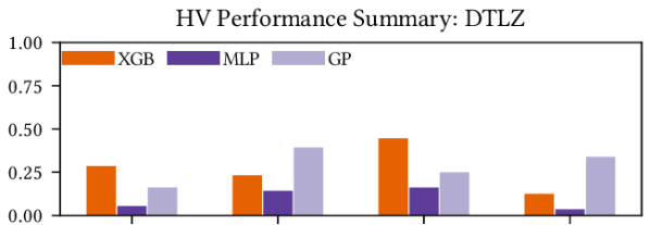
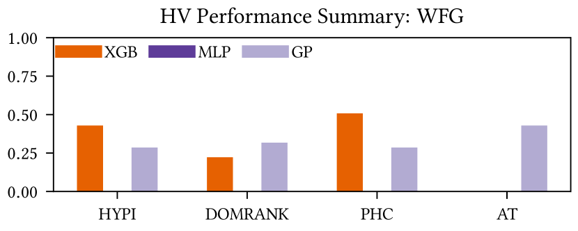
Figure 1. Hypervolume (HV) performance summary for the DTLZ and WFG benchmarks. Bar heights correspond to the proportion of times that a model and scalariser combination is best or statistically equivalent to the best method.

Given that Table 2 only compares performance between models for a given scalarisation, we now evaluate which combination of scalarisation and model performs the best on both the DTLZ and WFG benchmarks. Figure 1 summarises the performance for all combinations of model and scalariser. Bar heights correspond to the proportion of times each model and scalarisation combination was the best on each test problem. As can be seen from the figure, MBORE with XGB and our novel PHC scalariser (15) has the best overall performance for both benchmarks. Surprisingly, MBORE with the MLP classification method performs worse than the best performing method on all the $63$ WFG test problems. However, this reflects the results presented in (Tiao et al., 2021) that also show that XGB tends outperform MLP. We note that relative rankings of methods remain the same when using IGD+; see the supplement for details.

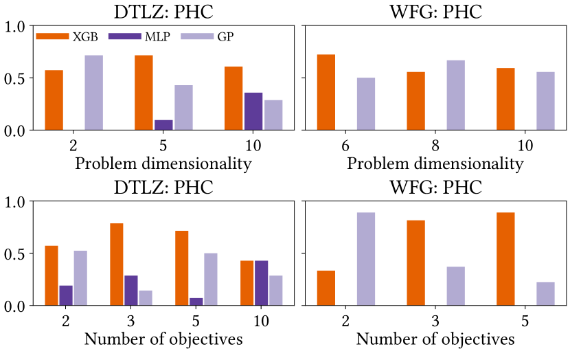
Figure 2. Hypervolume performance summary for the PHC scalariser on the DTLZ (left) and WFG (right) benchmarks given the problem’s dimensionality (upper) and number of objectives (lower).

Next, we investigate the performance of the models with respect to a problem’s dimensionality $d$ and number of objectives $M$. Since PHC was the best-performing method, we limit this discussion to its results. Results for all scalarisers are available in the supplement. Figure 2 summarises the performance of each combination of model and scalariser for the two benchmarks in terms of $d$ and $M$. The DTLZ results show that BO’s performance deteriorates as $d$ increases, a trend mirrored for the other scalarisations. Conversely, there is no clear pattern regarding $M$ for DLTZ. In the WFG benchmark the reverse is true, changing $d$ does not result in a consistent trend, but the performance of BO decreases and XGB increases as $M$ increases across the majority of scalarisation methods. We conjecture that this is related to the increased complexity of the WFG problems (Huband et al., 2006), compared to DTLZ. Therefore, increasing $M$ leads to an increase in the scalarisation landscape’s complexity, resulting in features that GPs model poorly, such as discontinuities.

5.2. Real-world Benchmark

Hand-crafted benchmarks, such as DTLZ and WFG, are known to have properties that are unlikely to appear in real-world applications (Ishibuchi et al., 2017; Zapotecas-Martínez et al., 2019). Therefore, to investigate the performance of MBORE in more realistic settings, we turn to the real-world benchmark of Tanabe and Ishibuchi (2020). It has $11$ continuous-valued test problems taken from real-world problems, such as car side impact design (Jain and Deb, 2014) and water resource planning (Ray et al., 2001); see (Tanabe and Ishibuchi, 2020) for detailed descriptions. The problem RE3-4-3 was not included due to numerical instabilities; we focus on the remaining $10$ problems.

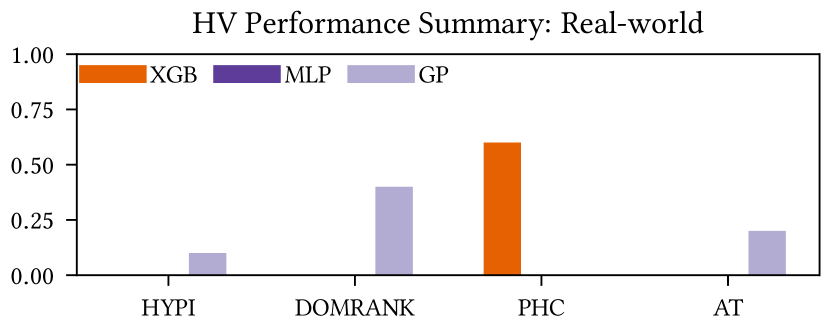
Figure 3. Hypervolume (HV) performance summary for the real-world benchmark problems. Bar heights correspond to the proportion of times that a model and scalariser combination is best or statistically equivalent to the best method.

Figure 3 summarises the performance of each combination of model and scalariser on the real-world problem benchmark. As can be seen from the figure, MBORE with XGB and using the PHC scalarisation is by far the best method for optimising the real-world problems based on hypervolume. Interestingly, for DomRank and AT, using BO (GP) was more effective than MBORE, with HYPI and PHC roughly equal between the two methods; see the supplement for full details. These results again show that using MBORE is suitable for multi-objective optimisation and outperforms BO when using more effective scalarisation methods.

5.3. High-dimensional Benchmark

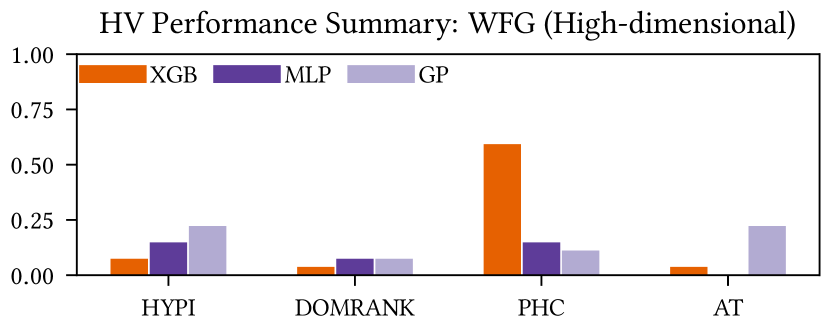
Figure 4. Hypervolume (HV) performance summary for the high-dimensional WFG benchmark. Bar heights correspond to the proportion of times that a model and scalariser combination is best or statistically equivalent to the best method.

BO often struggles on high-dimensional problems due to the surrogate models of choice, GPs, decreasing in modelling accuracy as the problem dimensionality increases (Györfi et al., 2002). Consequentially, comparisons of multi-objective methods often focus on lower numbers of both objectives $M$ and $d$. In contrast to this, and in order to evaluate MBORE in more realistic settings where both $d$ and $M$ are comparatively large, we investigate optimisation performance on the WFG benchmark (Huband et al., 2006) with a large dimensionality $d\in\{20,50,100\}$. Due to the computational costs of training GPs in high dimensions, we limit the number of objectives to one configuration ($M=10$); see the following section for a comparison of the computational costs.

Figure 4 summarises the performance on these problems. The efficacy of MBORE is repeated for the high-dimesional versions of the WFG problems, with the combination of MBORE, XGB and the PHC scalariser being the best on roughly two thirds of the problems. This is somewhat expected because, in the high-dimensional ($d\geq 20$) setting due to the aforementioned difficulties GPs can have with larger problem dimensions. Intriguingly, as shown in the supplement, the comparative performance for MLP-based MBORE increases with $d$ for all four scalarisations.

5.4. Computational Timing

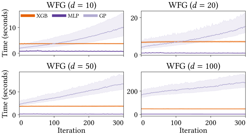
Figure 5. Computational time taken per iteration on the WFG benchmark for $d\in\{10,20,50,100\}$. The median computation time over all scalarisations is shown as the solid lines, with the corresponding interquartile ranges shaded.

We also investigate the computational performance of the three methods, MBORE with XGB and MLP, and BO with a GP surrogate model. The cost of performing one iteration of each method was recorded for all scalarisers on the WFG benchmark with $d\in\{10,20,50,100\}$. To ensure a fair comparison, each optimisation run was carried out on one core of an Intel Xeon E5-2640 v4 CPU. Figure 5 shows the timing results. The median computation time across all scalarisations for each iteration is shown, with shaded regions corresponding to the interquartile range. As theory necessarily dictates (Rasmussen and Williams, 2006), the GP’s computation time increases with the number of solutions. Conversely, the computation time of XGB and MLP are roughly constant for all iterations for a given dimensionality.

6. Conclusions

In this work, we presented MBORE: a novel multi-objective algorithm for expensive optimisation problems by scalarisation. It replaces the traditional mono-surrogate BO pipeline by training a probabilistic classifier on previously-evaluated solutions that were thresholded into two classes based on their objective value’s scalarised form. The classifier’s predictions can then be shown to approximate the probability of improving over the given threshold. In addition to MBORE, we also introduce PHC, a dominance-preserving scalarisation method that uses a modified form of each solution’s hypervolume contribution to its Pareto shell.

As demonstrated throughout, MBORE provides a strong alternative to mono-surrogate BO using GPs. This is particularly true for more difficult problems, such as the WFG and real-world benchmarks, as well as for problems with higher dimensionalities. Additionally, the computational costs of MBORE remain approximately constant as the number of solutions included in the model increases. We note that, we are not able to recommend MBORE over BO (or vice versa) for an arbitrary scalarisation, as shown by BO being consistently better with the AT scalarisation and MBORE with PHC. However, PHC consistently outperformed all other scalarisation methods. Therefore, we recommend the use of MBORE with XGB using the PHC scalarisation method as the new de facto choice for mono-surrogate-based multi-objective optimisation.

Future work includes extending MBORE to non-continuous spaces by using random forests. These are able to naturally adapt to discrete and categorical data without the need for, e.g. one-hot encoding. Additionally, we also seek to extend MBORE to the multi-surrogate setting by replacing its multiple GP models with one or more probabilistic classifiers, thereby substantially reducing computational complexity.

- (1)
- Balandat et al. (2020) Maximilian Balandat, Brian Karrer, Daniel Jiang, Samuel Daulton, Ben Letham, Andrew G. Wilson, and Eytan Bakshy. 2020. BoTorch: A Framework for Efficient Monte-Carlo Bayesian Optimization. Advances in Neural Information Processing Systems 33 (2020), 21524–21538.
- Belakaria et al. (2019) Syrine Belakaria, Aryan Deshwal, and Janardhan Rao Doppa. 2019. Max-value Entropy Search for Multi-Objective Bayesian Optimization. In Advances in Neural Information Processing Systems, Vol. 32. Curran Associates, Inc., 7825–7835.
- Bergstra et al. (2011) James Bergstra, Rémi Bardenet, Yoshua Bengio, and Balázs Kégl. 2011. Algorithms for Hyper-Parameter Optimization. In Advances in Neural Information Processing Systems, Vol. 24. Curran Associates, Inc., 281–305.
- Bickel et al. (2007) Steffen Bickel, Michael Brückner, and Tobias Scheffer. 2007. Discriminative learning for differing training and test distributions. In Proceedings of the 24th international conference on Machine learning. Association for Computing Machinery, New York, NY, USA, 81–88.
- Biscani and Izzo (2020) Francesco Biscani and Dario Izzo. 2020. A parallel global multiobjective framework for optimization: pagmo. Journal of Open Source Software 5, 53 (2020), 2338.
- Blank and Deb (2020) Julian Blank and Kalyanmoy Deb. 2020. Pymoo: Multi-Objective Optimization in Python. IEEE Access 8 (2020), 89497–89509.
- Blank et al. (2021) Julian Blank, Kalyanmoy Deb, Yashesh Dhebar, Sunith Bandaru, and Haitham Seada. 2021. Generating Well-Spaced Points on a Unit Simplex for Evolutionary Many-Objective Optimization. IEEE Transactions on Evolutionary Computation 25, 1 (2021), 48–60.
- Bull (2011) Adam D. Bull. 2011. Convergence Rates of Efficient Global Optimization Algorithms. Journal of Machine Learning Research 12, 88 (2011), 2879–2904.
- Byrd et al. (1995) Richard H. Byrd, Peihuang Lu, Jorge Nocedal, and Ciyou Zhu. 1995. A Limited Memory Algorithm for Bound Constrained Optimization. SIAM Journal on Scientific Computing 16, 5 (1995), 1190–1208.
- Chen and Guestrin (2016) Tianqi Chen and Carlos Guestrin. 2016. XGBoost: A Scalable Tree Boosting System. In Proceedings of the 22nd ACM SIGKDD International Conference on Knowledge Discovery and Data Mining (KDD ’16). Association for Computing Machinery, New York, NY, USA, 785–794.
- Cheng and Chu (2004) K. F. Cheng and C. K. Chu. 2004. Semiparametric density estimation under a two-sample density ratio model. Bernoulli 10, 4 (2004), 583–604.
- Chugh (2020) Tinkle Chugh. 2020. Scalarizing Functions in Bayesian Multiobjective Optimization. In 2020 IEEE Congress on Evolutionary Computation (CEC). IEEE, 1–8.
- Chugh et al. (2018) Tinkle Chugh, Yaochu Jin, Kaisa Miettinen, Jussi Hakanen, and Karthik Sindhya. 2018. A Surrogate-Assisted Reference Vector Guided Evolutionary Algorithm for Computationally Expensive Many-Objective Optimization. IEEE Transactions on Evolutionary Computation 22, 1 (2018), 129–142.
- Coello et al. (2006) Carlos A. Coello Coello, Gary B. Lamont, and David A. Van Veldhuizen. 2006. Evolutionary Algorithms for Solving Multi-Objective Problems (Genetic and Evolutionary Computation). Springer-Verlag, Berlin, Heidelberg.
- De Ath et al. (2021) George De Ath, Richard M. Everson, and Jonathan E. Fieldsend. 2021. How Bayesian should Bayesian optimisation be? In Proceedings of the Genetic and Evolutionary Computation Conference Companion. Association for Computing Machinery, New York, NY, USA, 1860–1869.
- De Ath et al. (2021) George De Ath, Richard M. Everson, Alma A. M. Rahat, and Jonathan E. Fieldsend. 2021. Greed is Good: Exploration and Exploitation Trade-offs in Bayesian Optimisation. ACM Transactions on Evolutionary Learning and Optimization 1, 1 (2021), 1–22.
- De Ath et al. (2020) George De Ath, Jonathan E. Fieldsend, and Richard M. Everson. 2020. What do you mean? The role of the mean function in Bayesian optimisation. In Proceedings of the Genetic and Evolutionary Computation Conference Companion. Association for Computing Machinery, New York, NY, USA, 1623–1631.
- Deb et al. (2005) Kalyanmoy Deb, Lothar Thiele, Marco Laumanns, and Eckart Zitzler. 2005. Scalable Test Problems for Evolutionary Multiobjective Optimization. In Evolutionary Multiobjective Optimization: Theoretical Advances and Applications. Springer, London, 105–145.
- Emmerich (2005) Michael T. M. Emmerich. 2005. Single- and multi-objective evolutionary design optimization assisted by Gaussian random field metamodels. Ph. D. Dissertation. TU Dortmund.
- Fleischer (2003) M. Fleischer. 2003. The measure of Pareto optima applications to multi-objective metaheuristics. In Proceedings of the 2nd international conference on Evolutionary multi-criterion optimization (EMO’03). Springer-Verlag, Berlin, Heidelberg, 519–533.
- Fonseca and Fleming (1993) Carlos M. Fonseca and Peter J. Fleming. 1993. Genetic Algorithms for Multiobjective Optimization: Formulation, Discussion and Generalization. In Proceedings of the 5th International Conference on Genetic Algorithms. Morgan Kaufmann Publishers Inc., San Francisco, CA, USA, 416–423.
- Frazier (2018) Peter I Frazier. 2018. A tutorial on Bayesian optimization. arXiv:1807.02811
- Gardner et al. (2017) Jacob Gardner, Chuan Guo, Kilian Weinberger, Roman Garnett, and Roger Grosse. 2017. Discovering and exploiting additive structure for Bayesian optimization. In Proceedings of the 20th international conference on artificial intelligence and statistics, Vol. 54. PMLR, 1311–1319.
- Gardner et al. (2018) Jacob Gardner, Geoff Pleiss, Kilian Q Weinberger, David Bindel, and Andrew G Wilson. 2018. GPyTorch: Blackbox Matrix-Matrix Gaussian Process Inference with GPU Acceleration. In Advances in Neural Information Processing Systems. Curran Associates, Inc., 7576–7586.
- Garnett (2022) Roman Garnett. 2022. Bayesian Optimization. Cambridge University Press. in preparation.
- Gneiting and Raftery (2007) Tilmann Gneiting and Adrian E Raftery. 2007. Strictly Proper Scoring Rules, Prediction, and Estimation. J. Amer. Statist. Assoc. 102, 477 (2007), 359–378.
- Guo et al. (2012) Guanqi Guo, Wu Li, Bo Yang, Wenbin Li, and Cheng Yin. 2012. Predicting Pareto Dominance in Multi-objective Optimization Using Pattern Recognition. In 2012 Second International Conference on Intelligent System Design and Engineering Application. IEEE, 456–459.
- Györfi et al. (2002) László Györfi, Michael Kohler, Adam Krzyzak, and Harro Walk. 2002. A Distribution-Free Theory of Nonparametric Regression. Springer.
- Hansen (2009) Nikolaus Hansen. 2009. Benchmarking a BI-population CMA-ES on the BBOB-2009 function testbed. In Proceedings of the 11th Annual Conference Companion on Genetic and Evolutionary Computation Conference: Late Breaking Papers (GECCO ’09). Association for Computing Machinery, New York, NY, USA, 2389–2396.
- Hennig and Schuler (2012) Philipp Hennig and Christian J. Schuler. 2012. Entropy Search for Information-Efficient Global Optimization. Journal of Machine Learning Research 13, 1 (2012), 1809–1837.
- Henrández-Lobato et al. (2014) José Miguel Henrández-Lobato, Matthew W. Hoffman, and Zoubin Ghahramani. 2014. Predictive Entropy Search for Efficient Global Optimization of Black-Box Functions. In Advances in Neural Information Processing Systems. MIT Press, 918–926.
- Holm (1979) Sture Holm. 1979. A simple sequentially rejective multiple test procedure. Scandinavian Journal of Statistics 6, 2 (1979), 65–70.
- Hornik et al. (1989) Kurt Hornik, Maxwell Stinchcombe, and Halbert White. 1989. Multilayer feedforward networks are universal approximators. Neural Networks 2, 5 (1989), 359–366.
- Huband et al. (2006) S. Huband, P. Hingston, L. Barone, and L. While. 2006. A review of multiobjective test problems and a scalable test problem toolkit. IEEE Transactions on Evolutionary Computation 10, 5 (2006), 477–506.
- Hutter et al. (2011) Frank Hutter, Holger H. Hoos, and Kevin Leyton-Brown. 2011. Sequential model-based optimization for general algorithm configuration. In Proceedings of the 5th international conference on Learning and Intelligent Optimization. Springer-Verlag, Berlin, Heidelberg, 507–523.
- Hwang and Masud (1979) Ching-Lai Hwang and Abu Syed Md. Masud. 1979. Multiple objective decision making, methods and applications : a state-of-the-art survey. Berlin ; New York : Springer-Verlag.
- Ishibuchi et al. (2015) Hisao Ishibuchi, Hiroyuki Masuda, Yuki Tanigaki, and Yusuke Nojima. 2015. Modified Distance Calculation in Generational Distance and Inverted Generational Distance. In Evolutionary Multi-Criterion Optimization. Springer International Publishing, Berlin, Heidelberg, 110–125.
- Ishibuchi et al. (2017) Hisao Ishibuchi, Yu Setoguchi, Hiroyuki Masuda, and Yusuke Nojima. 2017. Performance of Decomposition-Based Many-Objective Algorithms Strongly Depends on Pareto Front Shapes. IEEE Transactions on Evolutionary Computation 21, 2 (2017), 169–190.
- Jain and Deb (2014) Himanshu Jain and Kalyanmoy Deb. 2014. An Evolutionary Many-Objective Optimization Algorithm Using Reference-Point Based Nondominated Sorting Approach, Part II: Handling Constraints and Extending to an Adaptive Approach. IEEE Transactions on Evolutionary Computation 18, 4 (2014), 602–622.
- Jiang et al. (2020) Shan Jiang, Hongyan Zhang, Wenfeng Cong, Zhengyuan Liang, Qiran Ren, Chong Wang, Fusuo Zhang, and Xiaoqiang Jiao. 2020. Multi-Objective Optimization of Smallholder Apple Production: Lessons from the Bohai Bay Region. Sustainability 12, 16 (2020), 6496.
- Joachims (2005) Thorsten Joachims. 2005. A support vector method for multivariate performance measures. In Proceedings of the 22nd international conference on Machine learning (ICML ’05). Association for Computing Machinery, New York, NY, USA, 377–384.
- Jones et al. (1998) Donald R. Jones, Matthias Schonlau, and William J. Welch. 1998. Efficient Global Optimization of Expensive Black-Box Functions. Journal of Global Optimization 13, 4 (1998), 455–492.
- Kandasamy et al. (2015) Kirthevasan Kandasamy, Jeff Schneider, and Barnabas Poczos. 2015. High Dimensional Bayesian Optimisation and Bandits via Additive Models. In International Conference on Machine Learning. PMLR, 295–304.
- Knowles (2006) Josh Knowles. 2006. ParEGO: a hybrid algorithm with on-line landscape approximation for expensive multiobjective optimization problems. IEEE Transactions on Evolutionary Computation 10, 1 (2006), 50–66.
- Knowles et al. (2006) Joshua D. Knowles, Lothar Thiele, and Eckart Zitzler. 2006. A Tutorial on the Performance Assessment of Stochastic Multiobjective Optimizers. Technical Report TIK214. Computer Engineering and Networks Laboratory, ETH Zurich, Zurich, Switzerland.
- Kushner (1964) Harold J. Kushner. 1964. A new method of locating the maximum point of an arbitrary multipeak curve in the presence of noise. Journal Basic Engineering 86, 1 (1964), 97–106.
- Letham et al. (2020) Ben Letham, Roberto Calandra, Akshara Rai, and Eytan Bakshy. 2020. Re-examining linear embeddings for high-dimensional Bayesian optimization. In Advances in neural information processing systems, Vol. 33. Curran Associates, Inc., 1546–1558.
- Li et al. (2015) Bingdong Li, Jinlong Li, Ke Tang, and Xin Yao. 2015. Many-Objective Evolutionary Algorithms: A Survey. Comput. Surveys 48, 1 (2015), 1–35.
- Li and Lin (2007) Ling Li and Hsuan-tien Lin. 2007. Ordinal Regression by Extended Binary Classification. In Advances in Neural Information Processing Systems, Vol. 19. MIT Press, 865–872.
- Liao et al. (2019) Thomas Liao, Grant Wang, Brian Yang, Rene Lee, Kristofer Pister, Sergey Levine, and Roberto Calandra. 2019. Data-efficient Learning of Morphology and Controller for a Microrobot. In 2019 International Conference on Robotics and Automation (ICRA). IEEE, 2488–2494.
- Loshchilov et al. (2010a) Ilya Loshchilov, Marc Schoenauer, and Michèle Sebag. 2010a. Dominance-Based Pareto-Surrogate for Multi-Objective Optimization. In Simulated Evolution And Learning (SEAL-2010). Springer, Kanpur, India, 230–239.
- Loshchilov et al. (2010b) Ilya Loshchilov, Marc Schoenauer, and Michèle Sebag. 2010b. A mono surrogate for multiobjective optimization. In Proceedings of the 12th annual conference on Genetic and evolutionary computation. Association for Computing Machinery, New York, NY, USA, 471–478.
- McKay et al. (1979) M. D. McKay, R. J. Beckman, and W. J. Conover. 1979. A Comparison of Three Methods for Selecting Values of Input Variables in the Analysis of Output from a Computer Code. Technometrics 21, 2 (1979), 239–245.
- Menon and Ong (2016) Aditya Menon and Cheng Soon Ong. 2016. Linking losses for density ratio and class-probability estimation. In Proceedings of The 33rd International Conference on Machine Learning. PMLR, 304–313.
- Močkus et al. (1978) Jonas Močkus, Vytautas Tiešis, and Antanas Žilinskas. 1978. The application of Bayesian methods for seeking the extremum. Towards Global Optimization 2, 1 (1978), 117–129.
- Pan et al. (2019) Linqiang Pan, Cheng He, Ye Tian, Handing Wang, Xingyi Zhang, and Yaochu Jin. 2019. A Classification-Based Surrogate-Assisted Evolutionary Algorithm for Expensive Many-Objective Optimization. IEEE Transactions on Evolutionary Computation 23, 1 (2019), 74–88.
- Rahat et al. (2017) Alma A. M. Rahat, Richard M. Everson, and Jonathan E. Fieldsend. 2017. Alternative infill strategies for expensive multi-objective optimisation. In Proceedings of the Genetic and Evolutionary Computation Conference (GECCO ’17). Association for Computing Machinery, New York, NY, USA, 873–880.
- Rasmussen and Williams (2006) Carl Edward Rasmussen and Christopher K. I. Williams. 2006. Gaussian processes for machine learning. MIT Press, Cambridge, Massachusetts.
- Ray et al. (2001) Tapabrata Ray, Kang Tai, and Kin Chye Seow. 2001. Multiobjective Design Optimization by an Evolutionary Algorithm. Engineering Optimization 33, 4 (2001), 399–424.
- Rolland et al. (2018) Paul Rolland, Jonathan Scarlett, Ilija Bogunovic, and Volkan Cevher. 2018. High-Dimensional Bayesian Optimization via Additive Models with Overlapping Groups. In Proceedings of the Twenty-First International Conference on Artificial Intelligence and Statistics. PMLR, 298–307.
- Ru et al. (2018) Binxin Ru, Michael A. Osborne, Mark Mcleod, and Diego Granziol. 2018. Fast Information-Theoretic Bayesian Optimisation. In International Conference on Machine Learning. PMLR, 4384–4392.
- Salimbeni et al. (2018) Hugh Salimbeni, Ching-An Cheng, Byron Boots, and Marc Deisenroth. 2018. Orthogonally Decoupled Variational Gaussian Processes. In Advances in Neural Information Processing Systems, Vol. 31. Curran Associates, Inc., 8711–8720.
- Scott et al. (2011) Warren Scott, Peter Frazier, and Warren Powell. 2011. The Correlated Knowledge Gradient for Simulation Optimization of Continuous Parameters using Gaussian Process Regression. SIAM Journal on Optimization 21, 3 (2011), 996–1026.
- Seah et al. (2012) Chun-Wei Seah, Yew-Soon Ong, Ivor W. Tsang, and Siwei Jiang. 2012. Pareto Rank Learning in Multi-objective Evolutionary Algorithms. In 2012 IEEE Congress on Evolutionary Computation. IEEE, 1–8.
- Shahriari et al. (2016) Bobak Shahriari, Kevin Swersky, Ziyu Wang, Ryan P. Adams, and Nando de Freitas. 2016. Taking the human out of the loop: A review of Bayesian optimization. Proc. IEEE 104, 1 (2016), 148–175.
- Shi et al. (2020) Jiaxin Shi, Michalis Titsias, and Andriy Mnih. 2020. Sparse Orthogonal Variational Inference for Gaussian Processes. In Proceedings of the Twenty Third International Conference on Artificial Intelligence and Statistics. PMLR, 1932–1942.
- Silverman (1986) Bernard W. Silverman. 1986. Density Estimation for Statistics and Data Analysis. CRC Press.
- Snelson and Ghahramani (2006) Edward Snelson and Zoubin Ghahramani. 2006. Sparse Gaussian Processes using Pseudo-inputs. In Advances in Neural Information Processing Systems, Vol. 18. MIT Press, 1257–1264.
- Snoek et al. (2012) Jasper Snoek, Hugo Larochelle, and Ryan P Adams. 2012. Practical Bayesian Optimization of Machine Learning Algorithms. In Advances in Neural Information Processing Systems. Curran Associates, Inc., New York, 2951–2959.
- Snoek et al. (2015) Jasper Snoek, Oren Rippel, Kevin Swersky, Ryan Kiros, Nadathur Satish, Narayanan Sundaram, Mostofa Patwary, Mr Prabhat, and Ryan Adams. 2015. Scalable Bayesian Optimization Using Deep Neural Networks. In Proceedings of the 32nd International Conference on Machine Learning. PMLR, 2171–2180.
- Song and Ermon (2021) Jiaming Song and Stefano Ermon. 2021. Likelihood-free Density Ratio Acquisition Functions are not Equivalent to Expected Improvements. In Bayesian Deep Learning Workshop at NeurIPS. 4 pages.
- Srinivas et al. (2010) Niranjan Srinivas, Andreas Krause, Sham Kakade, and Matthias Seeger. 2010. Gaussian Process Optimization in the Bandit Setting: No Regret and Experimental Design. In International Conference on Machine Learning. Omnipress, 1015–1022.
- Stein (1999) Michael L. Stein. 1999. Interpolation of Spatial Data. Springer New York, New York.
- Sugiyama et al. (2012) Masashi Sugiyama, Taiji Suzuki, and Takafumi Kanamori. 2012. Density Ratio Estimation in Machine Learning. Cambridge University Press.
- Suzuki et al. (2020) Shinya Suzuki, Shion Takeno, Tomoyuki Tamura, Kazuki Shitara, and Masayuki Karasuyama. 2020. Multi-objective Bayesian Optimization using Pareto-frontier Entropy. In Proceedings of the 37th International Conference on Machine Learning. PMLR, 9279–9288.
- Tanabe and Ishibuchi (2020) Ryoji Tanabe and Hisao Ishibuchi. 2020. An easy-to-use real-world multi-objective optimization problem suite. Applied Soft Computing 89 (2020), 106078.
- Terrell and Scott (1992) George R. Terrell and David W. Scott. 1992. Variable Kernel Density Estimation. The Annals of Statistics 20, 3 (1992), 1236–1265.
- Tiao et al. (2021) Louis C Tiao, Aaron Klein, Matthias W Seeger, Edwin V. Bonilla, Cedric Archambeau, and Fabio Ramos. 2021. BORE: Bayesian Optimization by Density-Ratio Estimation. In Proceedings of the 38th International Conference on Machine Learning (Proceedings of Machine Learning Research, Vol. 139). PMLR, 10289–10300.
- Titsias (2009) Michalis Titsias. 2009. Variational Learning of Inducing Variables in Sparse Gaussian Processes. In Proceedings of the Twelfth International Conference on Artificial Intelligence and Statistics. PMLR, 567–574.
- Wang and Jegelka (2017) Zi Wang and Stefanie Jegelka. 2017. Max-Value Entropy Search for Efficient Bayesian Optimization. In International Conference on Machine Learning. PMLR, 3627–3635.
- Wang et al. (2017) Zi Wang, Chengtao Li, Stefanie Jegelka, and Pushmeet Kohli. 2017. Batched high-dimensional Bayesian optimization via structural kernel learning. In Proceedings of the 34th international conference on machine learning, Vol. 70. PMLR, 3656–3664.
- Wang et al. (2013) Ziyu Wang, Masrour Zoghi, Frank Hutter, David Matheson, and Nando De Freitas. 2013. Bayesian optimization in high dimensions via random embeddings. In Proceedings of the twenty-third international joint conference on artificial intelligence. AAAI Press, 1778–1784.
- Wilson and Nickisch (2015) Andrew Wilson and Hannes Nickisch. 2015. Kernel Interpolation for Scalable Structured Gaussian Processes (KISS-GP). In Proceedings of the 32nd International Conference on Machine Learning. PMLR, 1775–1784.
- Wilson et al. (2018) James Wilson, Frank Hutter, and Marc Deisenroth. 2018. Maximizing acquisition functions for Bayesian optimization. In Advances in Neural Information Processing Systems 31. Curran Associates, Inc., 9884–9895.
- Yamada et al. (2011) Makoto Yamada, Taiji Suzuki, Takafumi Kanamori, Hirotaka Hachiya, and Masashi Sugiyama. 2011. Relative Density-Ratio Estimation for Robust Distribution Comparison. In Advances in Neural Information Processing Systems, Vol. 24. Curran Associates, Inc., 594–602.
- Yang et al. (2019) Kaifeng Yang, Pramudita Satria Palar, Michael Emmerich, Koji Shimoyama, and Thomas Bäck. 2019. A multi-point mechanism of expected hypervolume improvement for parallel multi-objective Bayesian global optimization. In Proceedings of the Genetic and Evolutionary Computation Conference (GECCO ’19). Association for Computing Machinery, New York, NY, USA, 656–663.
- Yuan and Banzhaf (2021) Yuan Yuan and Wolfgang Banzhaf. 2021. Expensive Multi-Objective Evolutionary Optimization Assisted by Dominance Prediction. IEEE Transactions on Evolutionary Computation (2021). Early Access.
- Zapotecas-Martínez et al. (2019) Saúl Zapotecas-Martínez, Carlos A. Coello Coello, Hernán E. Aguirre, and Kiyoshi Tanaka. 2019. A Review of Features and Limitations of Existing Scalable Multiobjective Test Suites. IEEE Transactions on Evolutionary Computation 23, 1 (2019), 130–142.
- Zhang et al. (2018) Jinyuan Zhang, Aimin Zhou, Ke Tang, and Guixu Zhang. 2018. Preselection via classification: A case study on evolutionary multiobjective optimization. Information Sciences 465 (2018), 388–403.
- Zitzler (1999) Eckart Zitzler. 1999. Evolutionary Algorithms for Multiobjective Optimization: Methods and Applications. Ph. D. Dissertation. ETH Zurich.
- Zitzler and Künzli (2004) Eckart Zitzler and Simon Künzli. 2004. Indicator-Based Selection in Multiobjective Search. In Parallel Problem Solving from Nature - PPSN VIII (Lecture Notes in Computer Science). Springer, Berlin, Heidelberg, 832–842.