Adaptive estimation of random vectors with bandit feedback:
A mean-squared error viewpoint

Abstract

We consider the problem of sequentially learning to estimate, in the mean squared error (MSE) sense, a Gaussian $K$-vector of unknown covariance by observing only $m<K$ of its entries in each round. We first establish a concentration bound for MSE estimation. We then frame the estimation problem with bandit feedback, and propose a variant of the successive elimination algorithm. We also derive a minimax lower bound to understand the fundamental limit on the sample complexity of this problem.

1 Introduction

Several real-world applications involve collecting local measurements of a physical phenomenon, and then using the underlying correlation structure to form an estimate of the physical phenomenon over a wider region. For instance, using sensors to (i) monitor the temperature over a region (Guestrin et al., 2005)  and (ii) detect contamination in a water distribution network (Krause et al., 2008). Traffic monitoring in a cellular network is another application (Paul et al., 2014), where the underlying correlation structure plays a major role. In particular, the aim in this application is to collect traffic load measurements from a handful of base stations to form an estimate of the traffic load on all base stations.

In this paper we consider a setting where we have a $K$-dimensional Gaussian distribution with covariance matrix $\Sigma$, and the goal is to find a subset that best captures the underlying correlation structure. A Gaussian model for studying the correlation structure has been shown to be practically viable in (Paul et al., 2014). We employ the mean squared error (MSE) objective to capture the underlying correlation structure. For a $m$-subset $A$, the MSE $\psi(A)$ is given by

$$\psi(A)=\mathrm{Tr}\left(\Sigma_{A^{\prime}A^{\prime}}-\Sigma_{A^{\prime}A}\big{(}\Sigma_{AA}\big{)}^{-1}\Sigma_{AA^{\prime}}\right),$$ (1)

where $A^{\prime}$ is $[K]\setminus A$, and $\Sigma_{AA},\Sigma_{A^{\prime}A^{\prime}},\Sigma_{A^{\prime}A},\Sigma_{AA^{\prime}}$ are sub-matrices of $\Sigma$ in obvious notation, and $\mathrm{Tr}$ denote the trace function (See Section 2 for the details).

We first consider the problem of estimating the MSE of a $m$-subset, say $A$, given a batch of i.i.d. samples for each of the sub-matrices listed above. This problem is non-adaptive in the sense that each sub-matrix entry is pulled equally. An adaptive version of this problem is when we are provided entry-wise estimates of $\Sigma$, with non-uniform sampling. Such a set of samples facilitates estimation of MSE of any $m$-subset $A$.

From a statistical learning viewpoint, significant progress has been made on the problem of covariance matrix attention (cf. (Wainwright, 2019)). However, the problem of MSE estimation has not received enough attention, and there are no concentration bounds available for the problem of estimating (1), to the best of our knowledge. We propose a natural MSE estimator based on sample-averages for the non-adaptive as well as the adaptive settings. Since the sample average estimator of $\Sigma_{AA}$ may not be invertible, we perform an eigen-decomposition followed by projection of eigenvalues to the positive side. Next, we derive concentration bounds for the MSE estimation problem in the non-adaptive and adaptive settings. The bounds that we derive exhibit an exponential tail decay in either case.

We then frame the adaptive estimation problem with bandit feedback in the best-arm identification framework setting (Lattimore and Szepesvári, 2020). We apply the successive elimination technique (Even-Dar et al., 2002) to cater to the adaptive estimation problem. We present an upper bound on the sample complexity of this algorithm. Further, to understand the fundamental limit on the sample complexity of this adaptive estimation bandit problem, we derive an information-theoretic lower bound for the special case of $m=2$. We construct a set of covariance matrices that are rich enough to include the least favorable instance for any bandit algorithm. We establish the lower bound using the well-known standard change of measure argument by constructing problem transformations based on the aforementioned set of covariance matrices, but the technical steps require significant deviations in terms of algebraic effort. Moreover, the setting we consider involve sampling more than one arm, which is strictly necessary for estimating the underlying correlation. This sampling change implies additional effort in computing certain KL-divergences, which are then related to the sub-optimality gap in MSEs.

Related work. Previous works such as (Liu and Bubeck, 2014; Boda and Prashanth, 2019; Gupta et al., 2020) feature bandit formulations where the underlying correlation structure appears in the objective. In (Liu and Bubeck, 2014), the aim is to find the maximum correlated subset, i.e., a set that has highly correlated members. In contrast, our goal is to find a subset that best captures information about other, as quantified by the MSE objective. In addition, unlike (Liu and Bubeck, 2014), we do not assume unit variances in the underlying model. Next, in (Boda and Prashanth, 2019), which is the closest related work, the authors propose an MSE-based objective for a simplified version of the problem where the goal is to find an arm (or $1$-subset) that is most correlated to the remaining $K-1$ arms in the MSE sense. Our problem formulation is more general as we consider MSE of $m$-subsets, with $1\leq m\leq K$. This generalization leads to bigger technical challenges in MSE estimation and concentration, as well as in the lower bound analysis. Finally, in (Gupta et al., 2020), the authors assume that the arms are correlated through a latent random source, and the objective is to identify the arm with the highest mean. In (Erraqabi et al., 2017), the authors study the impact of correlation on the regret, while featuring a regular bandit formulation, i.e.. of identifying the arm with the highest mean.

The rest of the paper is organized as follows: In Section 2, we formally define the notion of MSE. In Sections 3 and  4, we describe MSE estimation in the non-adaptive and adaptive settings, respectively. In Section 5, we formulate the adaptive MSE estimation problem with bandit feedback, and we present a variant of successive elimination algorithm for solving this problem. In Section 6, we present a minimax lower bound on the sample complexity of the adaptive estimation problem in a BAI framework. In Section 7, we present the detailed proofs for the theoretical results in Sections 3–6. In Section 8, we present numerical experiments for MSE estimation and the bandit application. Finally, in Section 9 we provide our concluding remarks.

2 Preliminaries

We consider a jointly Gaussian $K$-vector $X=(X_{1},\ldots,X_{K})$, with mean zero and covariance matrix $\Sigma\triangleq\mathbb{E}[X^{\mathsf{\scriptscriptstyle T}}X]$:

$$\Sigma=\!\left[\!\begin{array}[]{c c c c}\sigma^{2}_{1}&\rho_{12}\sigma_{1}\sigma_{2}&\ldots&\rho_{1K}\sigma_{1}\sigma_{K}\\ \rho_{12}\sigma_{1}\sigma_{2}&\sigma^{2}_{2}&\ldots&\rho_{2K}\sigma_{2}\sigma_{K}\\ \vdots&\vdots&\ddots&\vdots\\ \rho_{1K}\sigma_{1}\sigma_{K}&\rho_{2K}\sigma_{2}\sigma_{K}&\ldots&\sigma^{2}_{K}\end{array}\!\right],\!$$ (6)

where $\sigma^{2}_{i}$, $i\in[K]$ is the variance of arm $i$ and $\rho_{ij}$, $i,j=1,\ldots,K,\ i\neq j,$ the correlation coefficient between arms $i$ and $j$. Here $[n]=\{1,\ldots,n\}$, for any natural number $n$.

Let $\mathcal{A}$ denote the set of subsets of $[K]$ with cardinality $m$. The mean-squared error (MSE) for a given subset
$A=\{i_{1},\ldots,i_{m}\}\in\mathcal{A}$ is defined as

$$\psi(A) \triangleq\sum_{j=1}^{K}\mathbb{E}[(X_{j}-\mathbb{E}[X_{j}|X_{i_{1}},\ldots,X_{i_{m}}])^{2}].$$ (7)

As shown by Hajek (2009), the above definition is equivalent to

$$\mathcal{\psi}(A)=\mathrm{Tr}\left(\Sigma_{A^{\prime}A^{\prime}}-\Sigma_{A^{\prime}A}\big{(}\Sigma_{AA}\big{)}^{-1}\Sigma_{AA^{\prime}}\right),$$ (8)

where $\mathrm{Tr}$ denotes the trace function, $A^{\prime}=[K]\setminus A$ is the complement of $A$, $\Sigma_{A^{\prime}A^{\prime}}$ (resp. $\Sigma_{AA}$) is the covariance matrix, which is obtained by restricting $\Sigma$ to the set $A^{\prime}$ (resp. $A$).

In next two sections, we describe the MSE estimation problem in the non-adaptive and adaptive settings, respectively. Subsequently, we present upper and lower bounds for the correlated bandit problem with an MSE objective.

3 Non-adaptive estimation

To estimate $\mathcal{\psi}(A)$, it is apparent from (8) that we require an estimate of the sub-matrices $\Sigma_{AA},\Sigma_{A^{\prime}A},\Sigma_{AA^{\prime}}$, and $\Sigma_{A^{\prime}A^{\prime}}$. In the non-adaptive setting, we are given i.i.d. samples for each of the sub-matrices $\Sigma_{AA},\Sigma_{A^{\prime}A^{\prime}},\Sigma_{A^{\prime}A},$ and $\Sigma_{AA^{\prime}}$, for a given subset $A$. Using these samples from the underlying multivariate Gaussian distribution, we form the sample covariance matrices $\widehat{\Sigma}_{AA}$, $\widehat{\Sigma}_{AA^{\prime}}$, $\widehat{\Sigma}_{A^{\prime}A}$, and $\widehat{\Sigma}_{A^{\prime}A^{\prime}}$ to estimate the aforementioned four sub-matrices.

The ‘sample-average’ estimator $\widehat{\Sigma}_{AA}$ is not guaranteed to be invertible (though it is positive definite with high probability), while MSE estimation requires an estimate of $\Sigma_{AA}^{-1}$. To handle invertibility, we form the matrix $\widehat{\Sigma_{AA}}^{+}$ by performing an eigen-decomposition of $\widehat{\Sigma}_{AA}$, followed by a projection of eigenvalues to the positive side. Formally, for $i=1,\ldots,m$, let $\hat{\lambda}_{i}$ denote the eigenvalue of $\widehat{\Sigma}_{AA}$, with corresponding eigenvector $v_{i}$. The estimator $\widehat{\Sigma}^{+}_{AA}$ is defined by

$$\widehat{\Sigma}_{AA}^{+}\triangleq\sum\limits_{i=1}^{m}\hat{\lambda}_{i}^{+}v_{i}v_{i}^{\intercal},$$ (9)

where $\hat{\lambda}_{i}^{+}=\begin{cases}\hat{\lambda}_{i}&\textrm{ if }|\hat{\lambda}_{i}|\geq\zeta,\\ \zeta&\textrm{otherwise},\end{cases}$ for $i=1,\ldots,m$. It is easy to see that $\widehat{\Sigma}_{AA}^{+}$ is positive definite.

The MSE $\psi(A)$ associated with set $A$ is then estimated as follows:

$$\widehat{\mathcal{\psi}}(A)\triangleq\mathrm{Tr}\left(\widehat{\Sigma_{A^{\prime}A^{\prime}}}-\widehat{\Sigma_{A^{\prime}A}}\big{(}\widehat{\Sigma_{AA}}^{+}\big{)}^{-1}\widehat{\Sigma_{AA^{\prime}}}\right).$$ (10)

Next, we proceed to analyze the concentration properties of the estimator defined above. For the sake of analysis, we make the following assumptions:

(A1).

$0<l=\underset{i}{\min}\;\sigma_{i}^{2},\sigma_{i}^{2}\leq 1$ for $i=1,\ldots,K$.

(A2).

$\max\left(||\Sigma_{AA}||_{2},||\Sigma_{A^{\prime}A^{\prime}}||_{2}\right)\leq M_{0},$ and $||\Sigma_{AA}^{-1}||_{2}\leq\frac{1}{M_{1}}$, where $||\cdot||_{2}$ is the operator norm.

Assumption (A1) is used for the simpler $1$-subset MSE estimation by Boda and Prashanth (2019), while (A2) is common in the analysis of covariance matrix estimates (cf. Cai et al. (2010)). We now present a concentration bound for the MSE estimator (10).

Proposition 1 (MSE concentration: Non-adaptive case).

Assume (A1) and (A2). Let $n_{AA},n_{A^{\prime}A},n_{AA^{\prime}},n_{A^{\prime}A^{\prime}}$ denote the number of samples used to form $\widehat{\Sigma}_{AA},\widehat{\Sigma}_{A^{\prime}A},\widehat{\Sigma}_{AA^{\prime}}$, and $\widehat{\Sigma}_{A^{\prime}A^{\prime}}$, respectively. Set the projection parameter $\zeta$ in (9) as follows:

$$\zeta=M_{0}\min\bigg{(}\sqrt{\frac{m+\log(\frac{1}{\delta})}{n_{AA}}},\frac{m+\log(\frac{1}{\delta})}{n_{AA}}\bigg{)}.$$

where $\delta\in(0,1)$ denotes the confidence width. Let $n^{\prime}=\min\left(n_{AA},n_{A^{\prime}A^{\prime}},n_{AA^{\prime}},n_{A^{\prime}A}\right)$.

Then, for any $0<\epsilon<\eta\triangleq\min\left(2K,\lambda_{min}(\Sigma_{AA})\right)$, the MSE estimate $\widehat{\mathcal{\psi}}(A)$ defined by (10) satisfies

$$\mathbb{P}\left(|\widehat{\mathcal{\psi}}(A)-\mathcal{\psi}(A)|\geq\epsilon\right)\leq\underbrace{C_{0}\exp\left(\frac{-n^{\prime}}{mK^{2}(1+\eta)^{3}}\min\left(\frac{\epsilon}{12G_{0}},\frac{\epsilon^{2}}{G_{0}^{2}}\right)\right)}_{(I)}+\underbrace{2mK\exp\left(-\frac{n^{\prime}\epsilon^{2}}{72\;C_{3}^{2}m^{2}K^{4}(1+\eta)^{3}}\right)}_{(II)},$$ (11)

where $c=\frac{1}{[\lambda_{\min}(\Sigma_{AA})-\epsilon]}$, $C_{0}=\left[13\text{ mK}+e^{m+K}\right],$ $C_{1}=\frac{108\sqrt{2}}{l}\left(c+\frac{1}{M_{1}}\right),$ $C_{2}=\bigg{(}\frac{3cM_{0}}{M_{1}}\bigg{)},$ $C_{3}=\left(c+\frac{1}{M_{1}}\right),$ and $G_{0}=\max\Big{(}\sqrt{m(K-m)^{2}}(1+\eta)\;C_{1},\sqrt{m(K-m)^{2}}(1+\eta)\;C_{2},3(K-m)M_{0}\Big{)}.$

Proof.

See Section 7.1. ∎

In the result above, we have $\epsilon\leq 2K$, and this constraint is not restrictive since the MSE $\psi(A)\leq K$ for any subset $A$ in lieu of (A1). A similar observation holds for the adaptive case handled later.

To understand the terms (I) and (II) in (11), we have to look at the following decomposition of the MSE estimation error:

$$\widehat{\mathcal{\psi}}(A)-\mathcal{\psi}(A) =\operatorname{\mathrm{Tr}}\left(\left(\widehat{\Sigma_{A^{\prime}A^{\prime}}}-\Sigma_{A^{\prime}A^{\prime}}\right)-\left(\widehat{\Sigma_{A^{\prime}A}}\left(\widehat{\Sigma_{AA}}^{+}\right)^{-1}\left(\widehat{\Sigma_{AA^{\prime}}}-\Sigma_{AA^{\prime}}\right)\right.\right.$$

$$\left.\left.\qquad\quad+\widehat{\Sigma_{A^{\prime}A}}\left(\left(\widehat{\Sigma_{AA}}^{+}\right)^{-1}-\Sigma_{AA}^{-1}\right)\Sigma_{AA^{\prime}}+\left(\widehat{\Sigma_{A^{\prime}A}}-\Sigma_{A^{\prime}A}\right)\Sigma_{AA}^{-1}\Sigma_{AA^{\prime}}\right)\right).$$ (12)

The first and third terms on the RHS above relate to estimation of a covariance matrix and its inverse. These terms lead to the term (I) in the bound (11) above. On the other hand the second and fourth terms on the RHS above relate to concentration of sample standard deviation and sample correlation coefficient, in turn leading to the term (II) in the bound (11).

4 Adaptive estimation

In the adaptive setting, we consider non-uniform sampling of the underlying covariance matrix, with the aim of reusing samples to estimate the MSE for different subsets.

The estimate in (10) is useful if one is concerned with estimating the MSE for a given subset. On the other hand, if one has to reuse sample information to estimate MSE for many subsets, then an approach that could be adopted is to maintain an estimate of each entry of the covariance matrix, and then, form MSE estimates for any subset by extracting the relevant information from the sample covariance matrix. We present a MSE estimation scheme based on this approach below.

For a subset $A=\{i_{1},\ldots,i_{m}\}$, the MSE $\psi(A)$, given in (8), can be re-written as follows:

$$\mathcal{\psi}(A)=\sum\limits_{j=1}^{K}\left[\sigma_{j}^{2}-C_{j}(\Sigma_{AA}^{-1})C_{j}^{\intercal}\right],$$ (13)

where $\Sigma_{AA}$ is as defined before, and $C_{j}=\left[\rho_{ji_{1}}\sigma_{i_{1}}\sigma_{j}\;\ldots\;\rho_{ji_{m}}\sigma_{i_{m}}\sigma_{j}\right]$. The MSE expressions in (7), (8) and (13) are equivalent. We have chosen to use (13) for adaptive estimation as it can be related easily to the MSE estimate presented below. Notice that, unlike the non-adaptive setting, the same sample set here can be used to estimate the MSE of any subset $A\in\mathcal{A}$.

From (13), it is apparent that one requires an estimate of the underlying variances, and correlation coefficients. Formally, we are given $n_{i}$ samples for the variance $\sigma_{i}^{2}$, and $n_{ij}$ samples for the correlation coefficient $\rho_{ij}$, $i,j\in[K],i\neq j$. The aim is to estimate (13) using these samples. For $j=1,\ldots,K$ and $k=1,\ldots,m$, let $\hat{\rho}_{j{i_{k}}}$ denote the sample correlation coefficient, and let $\hat{\sigma}_{j}^{2}$ denote the sample variance. These quantities are formed using $n_{j}$ and $n_{ji_{k}}$ samples, respectively, as follows:

$$\hat{\sigma}_{j}^{2}=\overline{X_{j}}^{2},\hat{\rho}_{j{i_{k}}}=\frac{\overline{X_{j}X_{i_{k}}}}{\hat{\sigma}_{j}\hat{\sigma}_{i_{k}}},\textrm{ where }\overline{X_{j}}^{2}=\frac{1}{n_{j}}\sum\limits_{t=1}^{n_{j}}X_{jt}^{2},\overline{X_{j}X_{i_{k}}}=\frac{1}{n_{ji_{k}}}\sum\limits_{t=1}^{n_{ji_{k}}}X_{jt}X_{i_{k}t}.$$

Using the sample variance and sample correlation coefficients, we estimate the MSE $\psi(A)$ as follows:

$$\widehat{\mathcal{\psi}}(A)=\sum\limits_{j=1}^{K}\left[\hat{\sigma}_{j}^{2}-\widehat{C_{j}}\big{(}\widehat{\Sigma_{AA}}^{+}\big{)}^{-1}\widehat{C_{j}}^{\intercal}\right].$$ (14)

$$\textrm{ where }\widehat{C_{j}}=\left[\hat{\rho}_{ji_{1}}\hat{\sigma}_{i_{1}}\hat{\sigma}_{j}\ldots\hat{\rho}_{j_{i_{m}}}\hat{\sigma}_{i_{m}}\hat{\sigma}_{j}\right],\widehat{\Sigma}_{AA}\textrm{ formed by using the relevant sample correlation coefficients }\hat{\rho}_{i_{k}i_{l}},$$

$$i_{k},i_{l}\in A,\textrm{ and sample variances }\hat{\sigma}_{i_{k}}^{2},i_{k}\in A,\textrm{ and }\widehat{\Sigma}_{AA}^{+}\textrm{ is defined in }\eqref{eq:sigma-hat-plus}.$$

Under the assumptions that are identical to the non-adaptive setting, we present a concentration bound for the MSE estimator (14) in the result below.

Proposition 2 (MSE concentration: Adaptive case).

Assume (A1) and (A2). Set the projection parameter $\zeta$ in (9) as follows:

$$\zeta =\sqrt{\frac{(1+\eta)^{3}(m^{2}-m)}{n^{\prime\prime}l^{2}}}\sqrt{\log\left(\frac{15(m^{2}-m)}{\delta}\right)}+\sqrt{\frac{m\log\left(\frac{m}{\delta}\right)}{n^{\prime\prime}}},$$

where $\delta\in(0,1)$ denotes the confidence width, $\eta\triangleq\min\left(2K,\lambda_{min}(\Sigma_{AA})\right)$. Then, for any $0<\epsilon<\eta$, the MSE estimate formed using (14) satisfies

$$\mathbb{P}\left(|\widehat{\mathcal{\psi}}(A)-\mathcal{\psi}(A)|\geq\epsilon\right) \leq\,14mK\exp\left(-\frac{n^{\prime\prime}}{G_{1}}\min\left(\frac{l\epsilon}{12\sqrt{2}\;G_{2}},\frac{l^{2}\epsilon^{2}}{G_{2}^{2}\;m(1+\eta)^{2}}\right)\right)$$

$$\qquad+30m^{2}K\exp\left(-\frac{n^{\prime\prime}l^{2}\epsilon^{2}}{G_{3}\;(m^{4}-m^{2})(1+\eta)^{7}}\right),$$ (15)

where $n^{\prime\prime}=\min\left(n_{i},n_{j},n_{ij},(i,j)\in[K],i\neq j\right)$, $C_{4}$ is a universal constant. $C_{5}=160\left(c+\frac{1}{M_{1}}\right),$ $C_{6}=\bigg{(}\frac{3c}{M_{1}}\bigg{)},$ $C_{7}=\left(c+\frac{1}{M_{1}}\right)$ , $G_{1}=\max\left(8,m(1+\eta)^{3}\right)$, $G_{2}=\max\left(1,C_{5}\right)$, and $G_{3}=\max\left(C_{4},\;C_{4}\;C_{6}^{2},\;72\;C_{7}^{2}\right)$.

Proof.

See Section 7.2. ∎

5 Adaptive estimation with bandit feedback

We consider the fixed confidence variant of the best-arm identification framework (Lattimore and Szepesvári, 2020). In this setting, the interaction of a bandit algorithm with the environment is given below.

Adaptive estimation with bandit feedback Input: set of $m$-subsets $\mathcal{A}$. For all $t=1,2,\ldots,$ repeat 1. Select an $m$-subset $A_{t}\in\mathcal{A}$. 2. Observe a sample from the multi-variate Gaussian distribution corresponding to the arms in the set $A_{t}$. 3. Choose to continue, or stop and output an $m$-subset.

A subset that has the lowest MSE is considered optimal, i.e.,

$$A^{*}\in\operatorname*{arg\,min}\limits_{A\in\mathcal{A}}\mathcal{\psi}(A).$$

The aim in this setting is to devise an algorithm that outputs the best $m$-subset with high probability, while using a low number of samples. More precisely, for a given confidence parameter $\delta\in(0,1)$, an algorithm is $\delta$-PAC if it stops after $\tau$ rounds, and outputs a set $A_{\tau}$ that satisfies $\mathbb{P}\left(A_{\tau}\neq A^{*}\right)\leq\delta$. Among $\delta$-PAC algorithms, the algorithm with minimum sample complexity $\mathbb{E}[\tau]$ is preferred.

For any set $A$, define

$$\Delta(A)\triangleq\psi(A)-\psi(A^{*}),\textrm{ and }\Delta=\min_{A\in\mathcal{A}}\Delta(A).$$ (16)

In the above, $\Delta(A)$ denotes the gap in MSE associated with a subset $A$, while $\Delta$ denotes the smallest gap. The upper and lower bounds that we derive subsequently features these quantities. In the fixed confidence setting that we consider, a naive algorithm based on Algorithm 1 in (Even-Dar et al., 2002) would pull each subset equal number of times. Such an uniform sampling will be useful if all the subsets can capture the same amount of information about other subsets, i.e., when the underlying correlations and the variances are similar. However, with uneven correlations, uniform sampling does not make sense. The possible set of candidates for the most informative subset need to sampled more than the other subsets in order to reduce the probability of error in identifying the best $m$-subset, and successive elimination (Even-Dar et al., 2002) is an approach that embodies this idea.

We propose a variant of the successive elimination algorithm that is geared towards finding the best $m$- subset under the MSE objective. The algorithm maintains an active set, which is initialized to the set of all $m$-subsets $\mathcal{A}$. In each round $t$, the algorithm pulls each active $m$-subset once, and its MSE is estimated using (14). Following this, the algorithm eliminates all subsets whose confidence intervals are clearly separated from the confidence interval of the empirically best subset seen so far, i.e., the one with the least MSE estimate. The algorithm terminates when there is only one $m$-subset left in the active set, and this event occurs with probablity one.

For deriving the confidence width $\alpha_{t}$ used in the successive elimination algorithm for correlated bandits (see Figure 1 below), we start by deriving an alternative form of the bound on the MSE estimate stated in Proposition 2.

$$\mathbb{P}\left(|\widehat{\mathcal{\psi}}(A)-\mathcal{\psi}(A)|\geq\epsilon\right) \leq K\left(\left(13m+1\right)\exp\left(-\frac{n^{\prime\prime}}{G_{1}}\min\left(\frac{l\epsilon}{12\sqrt{2}\;G_{2}},\frac{l^{2}\epsilon^{2}}{G_{2}^{2}\;m(1+\eta)^{2}}\right)\right)\right.$$

$$\quad\left.+\left(30m^{2}-26m\right)\exp\left(-\frac{n^{\prime\prime}l^{2}\epsilon^{2}}{G_{3}\;(m^{4}-m^{2})(1+\eta)^{7}}\right)\right)$$

$$\leq K\left(\left(13m+1\right)\exp\left(-\frac{n^{\prime\prime}l^{2}\epsilon^{2}}{12\sqrt{2}\;l\;G_{1}G_{2}\epsilon+G_{1}G_{2}^{2}\;m(1+\eta)^{2}}\right)\right.$$

$$\qquad\left.+\left(30m^{2}-26m\right)\exp\left(-\frac{n^{\prime\prime}l^{2}\epsilon^{2}}{G_{3}\;(m^{4}-m^{2})(1+\eta)^{7}}\right)\right)$$

$$\leq K\left(\left(13m+1\right)\exp\left(-\frac{n^{\prime\prime}\;\epsilon^{2}}{c_{1}+c_{2}\epsilon}\right)+\left(30m^{2}-26m\right)\exp\left(-n^{\prime\prime}c_{3}\epsilon^{2}\right)\right)$$

$$\leq K\left(\left(30m^{2}-13m+1\right)\exp\left(-\frac{n^{\prime\prime}\;\min(c_{3},1)\;\epsilon^{2}}{c_{1}+c_{2}\epsilon}\right)\right),$$

where $c_{1}=\frac{G_{1}\;G_{2}^{2}\;m\;(1+\eta)^{2}}{l^{2}}$, $c_{2}=\frac{12\sqrt{2}\;G_{1}\;G_{2}}{l}$ and $c_{3}=\frac{l^{2}}{G_{2}\;\left(m^{4}-m^{2}\right)\;\left(1+\eta\right)^{7}}$.

Since $c_{3}\leq 1$, we have

$$\mathbb{P}\left(|\widehat{\mathcal{\psi}}(A)-\mathcal{\psi}(A)|\geq\epsilon\right)\leq K\left(\left(30m^{2}-13m+1\right)\exp\left(-\frac{n^{\prime\prime}c_{3}\epsilon^{2}}{c_{1}+c_{2}\epsilon}\right)\right).$$ (17)

From (17), w.p. $1-\delta$, we obtain

$$|\widehat{\mathcal{\psi}}(A)-\mathcal{\psi}(A)|\leq\left(\frac{c_{2}\log\left(\frac{K\left(30m^{2}-13m+1\right)}{\delta}\right)}{n^{\prime\prime}c_{3}}+\sqrt{\frac{c_{1}\log\left(\frac{K\left(30m^{2}-13m+1\right)}{\delta}\right)}{n^{\prime\prime}c_{3}}}\right).$$ (18)

Now, from (18), we obtain the following form for the confidence width $\alpha_{t}$, which is used in the successive elimination algorithm for correlated bandits (see Figure 1 below):

$$\alpha_{t}=\left(\frac{c_{2}\log\left(\frac{70\;\binom{K}{m}Km^{2}t^{2}}{\delta}\right)}{2c_{3}\;t}+\sqrt{\frac{c_{1}\log\left(\frac{70\;\binom{K}{m}Km^{2}t^{2}}{\delta}\right)}{2c_{3}\;t}}\right).$$ (19)

Successive elimination for correlated bandits Input: set of all $m$-subsets $\mathcal{A},|\mathcal{A}|=\binom{K}{m},\delta>0$. Initialization: set of active subsets $\mathcal{S}=\mathcal{A}$ For all $t=1,2,\ldots$ , repeat
1. Select all active $m$-subsets $A_{t}\in\mathcal{S}$. 2. Observe a sample from the $m$-variate Gaussian distribution corresponding to the arms in each of the active sets $A_{t}$. 3. Remove those subsets from $\mathcal{S}$ such that
$\widehat{\psi}_{A_{t}^{*}}-\widehat{\psi}_{A_{t}}\geq 2\alpha_{t}$, where $\alpha_{t}$ is defined in (19) and $A_{t}^{*}$ is any active optimal subset at time $t$ with minimum MSE , i.e., $A_{t}^{*}\in\operatorname*{arg\,min}\limits_{A_{t}\in\mathcal{S}}\psi(A_{t}).$ 4. Continue until there is only one active $m$-subset in $\mathcal{S}$.

Figure 1: Operational flow of successive elimination for correlated bandits.

We now present a bound on the sample complexity of the successive elimination algorithm for correlated bandits.

Theorem 1 (Sample complexity bound).

Assume (A1) and (A2) for every $A\in\mathcal{A}$. The successive elimination algorithm is $(0,\delta)$-PAC for any $\delta\in(0,1)$, and w.p. at least $1-\delta$, it’s sample complexity is bounded by

$$\mathcal{O}\left(\sum\limits_{A\in\mathcal{A}}\frac{1}{\Delta(A)}\log\left(\frac{\binom{K}{m}Km^{2}\log\left(\Delta(A)^{-1}\right)}{\delta}\right)\right),$$

where $\Delta(A)$ is defined in (16).

Proof.

See Section 7.3. ∎

The sample complexity bound in the result above features the total number of $m$-subsets $\binom{K}{m}$, and is of the form $O\left(\frac{\binom{K}{m}}{\Delta}\log\left(\binom{K}{m}/\delta\right)\right)$, where $\Delta$ denotes the smallest gap. It is unclear if this bound can be improved without additional assumptions on the underlying covariance matrix $\Sigma$, and we believe the number of $m$-subsets $\binom{K}{m}$ has to appear in the sample complexity bound for a general covariance matrix $\Sigma$.

6 Lower Bound

We consider a special case of the adaptive estimation problem, where the goal is to identify the best pair of arms, i.e.,

$$(i_{1}^{*},i_{2}^{*})\in\operatorname*{arg\,min}\limits_{(i,j)\in[K]\times[K],i\neq j}\psi(\{i,j\}).$$

Let $Alg(\delta,K)$ denote the class of algorithms that are $\delta$-PAC for the best pair identification problem. A lower bound on the sample complexity of this problem is presented below.

Theorem 2 (Lower bound).

For any $\delta$-PAC algorithm, there exists a bandit problem instance governed by a covariance matrix $\Sigma$ such that the sample complexity $\mathbb{E}_{\Sigma}[\tau_{\delta}]$ of this algorithm satisfies

$$\mathbb{E}_{\Sigma}[\tau_{\delta}]\geq\frac{\log(\frac{1}{2.4\delta})}{\Delta}.$$ (20)

where $\Delta$ denotes the smallest gap on the problem instance governed by $\Sigma$.

Proof.

See Section 7.4. ∎

Comparing the lower bound to the upper bound for successive elimination in Theorem 1, we observe that the dependence on the minimum gap $\Delta$ is the same in either bound. However, the lower bound does not have a dependency on $m$ and $K$ through the number of arms $\binom{K}{m}$ — a dependency that is present in the upper bound. We believe the lower bound is sub-optimal from the dependence on the number of $m$-subsets (or arms), and it would be an interesting future direction of future work to establish a lower bound that involves the $\binom{K}{m}$ factor.

The proof strategy is to use the following class of covariance matrices parameterized by $\rho$:

$$\Sigma=\begin{bmatrix}1&\rho&\rho&\rho&\ldots&\rho\\ \rho&1&\rho^{2}&\rho^{2}&\ldots&\rho^{2}\\ \rho&\rho^{2}&1&\rho^{3}&\ldots&\rho^{3}\\ \vdots&\vdots&\vdots&\vdots&\ddots&\vdots\\ \rho&\rho^{2}&\rho^{3}&\ldots&\rho^{K-1}&1\end{bmatrix}$$ (21)

Using Sylvester’s criterion, it is easy to see that the matrix defined above is positive semi-definite.

For a $K$-armed Gaussian bandit instance with the underlying distribution governed by $\Sigma$ defined above, the pair $\{1,2\}$ has the least MSE.

We form $(2K-4)$ transformations of the bandit instance described in (21). The transformations are achieved by relabelling the $m^{th}$ row as either the first or second row of $\Sigma,m=3,\ldots,K.$ Let us denote the pdf associated with the original bandit instance by $\mathcal{G}$ and $\mathcal{G}^{km}$ is the probability density function (pdf) of the transformed bandit instance obtained by relabelling the $k^{th}(k=1\text{ or }2)$ row and the $m^{th}$ row of $\Sigma$.

The underlying covariance matrix for the problem instance corresponding to the $m$th transformation is $\Sigma_{km}$ with $m$th row re-labelled as either row 1 or 2.$\text{ Let }KL_{ij}^{km}\overset{\Delta}{=}KL(\nu_{i}\nu_{j}||\nu^{\prime}_{i}\nu^{\prime}_{j})$ specify the KL-divergence between $\nu_{i}\nu_{j}\text{ and }\nu^{\prime}_{i}\nu^{\prime}_{j}$, with the latter distribution derived from $\mathcal{G}^{km}.$

In the proof, we first show that

$$\underset{\{w_{ij}\}}{\min}\mathbb{E}[\tau_{\delta}]\geq\frac{\log(\frac{1}{2.4\delta})}{\underset{w\in\Delta_{\binom{K}{2}}}{\max}\underset{\Sigma^{\prime}\in\textrm{Alt}(\Sigma)}{\min}\sum\limits_{i,j}w_{ij}KL\left[\Sigma_{X_{i}X_{j}}||\Sigma^{\prime}_{X_{i}X_{j}}\right]},$$ (22)

where $\Delta_{\binom{K}{2}}$ is the set of probability distributions on the arm-pairs, and $\textrm{Alt}(\Sigma)=\{\Sigma^{1m},\Sigma^{2m},m>3\}$ is the set of transformed covariance matrices. While derivation of the inequality above is a straightforward variation to the proof in the classic bandit setting (cf. Kaufmann et al. (2015)), the rest of the proof in our case requires significant deviations. In particular, unlike the regular bandit case, the KL-divergences in the RHS above are not univariate. Moreover, deriving an upper bound on the max-min, which is defined in the RHS above, requires arguments that are specific to our correlated bandit setting.

We would like to note that Boda and Prashanth (2019) provide a lower bound for the correlated bandit problem with $m=1$. The proof of the lower bound for the case of $m=2$ is significantly different from the proof for $m=1$. In particular, it is challenging since the proof involves KL-divergences for bivariate distributions and relating these KL-divergences to the underlying gaps involves tools from optimization (see the proof sketch below), as well as significant algebraic effort to simplify KL-divergence bounds inside the max-min in (22), and then, relating the simplified expression to the gap in MSEs of the original problem instance. Further, unlike (Boda and Prashanth, 2019), the ideas in our proof for $m=2$ could be generalized to $m>2$.

7 Convergence proofs

7.1 Proof of Proposition 1

Proof.

Notice that

$$\widehat{\mathcal{\psi}}(A)-\mathcal{\psi}(A)=\mathrm{Tr}\bigg{(}\underbrace{\left(\widehat{\Sigma_{A^{\prime}A^{\prime}}}-\Sigma_{A^{\prime}A^{\prime}}\right)}_{(I)}-\underbrace{\bigg{(}\widehat{\Sigma_{A^{\prime}A}}\big{(}\widehat{\Sigma_{AA}}^{+}\big{)}^{-1}\widehat{\Sigma_{AA^{\prime}}}-\Sigma_{A^{\prime}A}\Sigma_{AA}^{-1}\Sigma_{AA^{\prime}}\bigg{)}}_{(II)}\bigg{)}.$$ (23)

The term (II) on the RHS of (23) can be re-written as follows:

$$(II) =\widehat{\Sigma_{A^{\prime}A}}\left(\widehat{\Sigma_{AA}}^{+}\right)^{-1}\widehat{\Sigma_{AA^{\prime}}}-\Sigma_{A^{\prime}A}\left(\Sigma_{AA}\right)^{-1}\Sigma_{AA^{\prime}}$$

$$=\widehat{\Sigma_{A^{\prime}A}}\left(\left(\widehat{\Sigma_{AA}}^{+}\right)^{-1}\widehat{\Sigma_{AA^{\prime}}}-\Sigma_{AA}^{-1}\Sigma_{AA^{\prime}}\right)+\left(\widehat{\Sigma_{A^{\prime}A}}-\Sigma_{A^{\prime}A}\right)\Sigma_{AA}^{-1}\Sigma_{AA^{\prime}}$$

$$=\widehat{\Sigma_{A^{\prime}A}}\left(\left(\widehat{\Sigma_{AA}}^{+}\right)^{-1}\left(\widehat{\Sigma_{AA^{\prime}}}-\Sigma_{AA^{\prime}}\right)+\left(\left(\widehat{\Sigma_{AA}}^{+}\right)^{-1}-\Sigma_{AA}^{-1}\right)\Sigma_{AA^{\prime}}\right)+\left(\widehat{\Sigma_{A^{\prime}A}}-\Sigma_{A^{\prime}A}\right)\Sigma_{AA}^{-1}\Sigma_{AA^{\prime}}$$

$$=\widehat{\Sigma_{A^{\prime}A}}\left(\widehat{\Sigma_{AA}}^{+}\right)^{-1}\left(\widehat{\Sigma_{AA^{\prime}}}-\Sigma_{AA^{\prime}}\right)+\widehat{\Sigma_{A^{\prime}A}}\left(\left(\widehat{\Sigma_{AA}}^{+}\right)^{-1}-\Sigma_{AA}^{-1}\right)\Sigma_{AA^{\prime}}+\left(\widehat{\Sigma_{A^{\prime}A}}-\Sigma_{A^{\prime}A}\right)\Sigma_{AA}^{-1}\Sigma_{AA^{\prime}}.$$ (24)

Using the definition of the positive definite estimator $\widehat{\Sigma}^{+}$, we have

$$||\widehat{\Sigma}_{AA}^{+}-\Sigma_{AA}||_{2} \leq||\widehat{\Sigma}_{AA}^{+}-\widehat{\Sigma}_{AA}||+||\widehat{\Sigma}_{AA}-\Sigma_{AA}||_{2}$$

$$\leq 2\zeta+||\widehat{\Sigma}_{AA}-\Sigma_{AA}||_{2}.$$ (25)

Using Theorem 5.7 of Rigollet and Hütter (2019) in conjunction with (A1), w.p. $(1-\delta)$, we have

$$||\widehat{\Sigma_{AA}}-\Sigma_{AA}||_{2} \leq||\Sigma_{AA}||_{2}\min\bigg{(}\sqrt{\frac{m+\log(\frac{1}{\delta})}{n_{AA}}},\frac{m+\log(\frac{1}{\delta})}{n_{AA}}\bigg{)}$$

$$\leq M_{0}\min\bigg{(}\sqrt{\frac{m+\log(\frac{1}{\delta})}{n_{AA}}},\frac{m+\log(\frac{1}{\delta})}{n_{AA}}\bigg{)}.$$ (26)

Along similar lines, we obtain

$$||\widehat{\Sigma_{A^{\prime}A^{\prime}}}-\Sigma_{A^{\prime}A^{\prime}}||_{2}\leq M_{0}\min\bigg{(}\sqrt{\frac{K-m+\log(\frac{1}{\delta})}{n_{A^{\prime}A^{\prime}}}},\frac{K-m+\log(\frac{1}{\delta})}{n_{A^{\prime}A^{\prime}}}\bigg{)}.$$ (27)

With $c=\frac{1}{[\lambda_{\min}(\Sigma_{AA})-\epsilon]}$, consider the event

$$\tilde{\mathcal{B}}= \{\sigma_{i}^{2}-\epsilon\leq\hat{\sigma}_{i}^{2}\leq\sigma_{i}^{2}+\epsilon,i=[K],\rho_{i_{k}j}-\epsilon\leq\hat{\rho}_{i_{k}j}\leq\rho_{i_{k}j}+\epsilon,\text{ for }(k,j)\in[K],k\neq j,||\left(\widehat{\Sigma}_{AA}^{+}\right)^{-1}||_{2}\leq c\}.$$ (28)

On the event $\tilde{\mathcal{B}}$, w.p. $(1-\delta)$, we have

$$||\left(\widehat{\Sigma_{AA}}^{+}\right)^{-1}-\Sigma_{AA}^{-1}||_{2} =||\left(\widehat{\Sigma}_{AA}\right)^{-1}\big{(}\Sigma_{AA}-\widehat{\Sigma_{AA}}^{+}\big{)}\Sigma_{AA}^{-1}||_{2}$$

$$\leq||\left(\widehat{\Sigma_{AA}}^{+}\right)^{-1}||_{2}\;||\Sigma_{AA}-\widehat{\Sigma_{AA}}^{+}||_{2}\;||\Sigma_{AA}^{-1}||_{2}$$

$$\leq\left(\frac{c}{M_{1}}\right)\left(2\zeta+M_{0}\min\bigg{(}\sqrt{\frac{m+\log(\frac{1}{\delta})}{n_{AA}}},\frac{m+\log(\frac{1}{\delta})}{n_{AA}}\bigg{)}\right)$$

$$=\frac{3cM_{0}}{M_{1}}\min\bigg{(}\sqrt{\frac{m+\log(\frac{1}{\delta})}{n_{AA}}},\frac{m+\log(\frac{1}{\delta})}{n_{AA}}\bigg{)},$$

where we used (25), (27), and substituted the value of $\zeta$ specified in the proposition statement.

Letting $\eta=\min\left(2K,\lambda_{min}(\Sigma_{AA})\right)$, we obtain $||\widehat{\Sigma_{AA^{\prime}}}||_{2}\leq\sqrt{m(K-m)}\left(1+\eta\right),\text{ since }\hat{\sigma}_{j}^{2}\leq\sigma_{j}^{2}+\epsilon\leq 1+\eta\text{ on }\tilde{\mathcal{B}}$ and $||\Sigma_{AA^{\prime}}||_{2}\leq\sqrt{m(K-m)}\left(1+\eta\right)$. Similarly, $||\widehat{\Sigma_{A^{\prime}A}}||_{2}\leq\sqrt{m(K-m)}(1+\eta)\text{ and }||\Sigma_{A^{\prime}A}||_{2}\leq\sqrt{m(K-m)}(1+\eta).$ Thus,

$$\mathbb{P}\left(||\widehat{\Sigma_{AA^{\prime}}}-\Sigma_{AA^{\prime}}||_{2}^{2}\geq\epsilon^{2},\tilde{\mathcal{B}}\right)$$

$$\leq\mathbb{P}\left(||\widehat{\Sigma_{AA^{\prime}}}-\Sigma_{AA^{\prime}}||_{F}^{2}\geq\epsilon^{2},\tilde{\mathcal{B}}\right)$$

$$=\sum\limits_{k=1}^{m}\sum\limits_{j=m+1}^{K-m}\mathbb{P}\bigg{(}|\hat{\rho}_{ji_{k}}\hat{\sigma}_{i_{k}}\hat{\sigma}_{j}-\rho_{ji_{k}}\sigma_{i_{k}}\sigma_{j}|\geq\frac{\epsilon}{\sqrt{m(K-m)}},\tilde{\mathcal{B}}\bigg{)}$$

$$=\sum\limits_{k=1}^{m}\sum\limits_{j=m+1}^{K-m}\mathbb{P}\bigg{(}|\hat{\rho}_{ji_{k}}\hat{\sigma}_{i_{k}}\left(\hat{\sigma}_{j}-\sigma_{j}\right)+\hat{\rho}_{ji_{k}}\sigma_{j}\left(\hat{\sigma}_{i_{k}}-\sigma_{i_{k}}\right)+\sigma_{i_{k}}\sigma_{i_{j}}\left(\hat{\rho}_{ji_{k}}-\rho_{ji_{k}}\right)|\geq\frac{\epsilon}{\sqrt{m(K-m)}},\tilde{\mathcal{B}}\bigg{)}$$

$$\leq\sum\limits_{k=1}^{m}\sum\limits_{j=m+1}^{K-m}\Bigg{(}\mathbb{P}\left(\hat{\rho}_{ji_{k}}\hat{\sigma}_{i_{k}}\left(\hat{\sigma}_{j}-\sigma_{j}\right)\geq\frac{\epsilon}{3\sqrt{m(K-m)}},\tilde{\mathcal{B}}\right)+\mathbb{P}\left(\hat{\rho}_{ji_{k}}\sigma_{j}\left(\hat{\sigma}_{i_{k}}-\sigma_{i_{k}}\right)\geq\frac{\epsilon}{3\sqrt{m(K-m)}},\tilde{\mathcal{B}}\right)$$

$$\qquad\qquad\qquad\qquad+\mathbb{P}\left(\sigma_{i_{k}}\sigma_{j}\left(\hat{\rho}_{ji_{k}}-\rho_{ji_{k}}\right)\geq\frac{\epsilon}{3\sqrt{m(K-m)}},\tilde{\mathcal{B}}\right)\Bigg{)}$$

$$\leq\sum\limits_{k=1}^{m}\sum\limits_{j=m+1}^{K-m}\Bigg{(}\mathbb{P}\left(\left(\hat{\sigma}_{j}-\sigma_{j}\right)\geq\frac{\epsilon}{3\sqrt{m(K-m)(1+\eta)}}\right)+\mathbb{P}\left(\left(\hat{\sigma}_{i_{k}}-\sigma_{i_{k}}\right)\geq\frac{\epsilon}{3\sqrt{m(K-m)(1+\eta)}}\right)\Bigg{.}$$

$$\qquad\qquad\qquad+\mathbb{P}\left(\big{(}\hat{\rho}_{ji_{k}}-\rho_{ji_{k}}\big{)}\geq\frac{\epsilon}{3\sqrt{m(K-m)}(1+\eta)},\tilde{\mathcal{B}}\right)\Bigg{)}$$

$$\leq\sum\limits_{k=1}^{m}\sum\limits_{j=m+1}^{K-m}\left(\exp\left(-\frac{n_{AA^{\prime}}\epsilon^{2}}{72m(K-m)(1+\eta)}\right)+\exp\left(-\frac{n_{AA^{\prime}}\epsilon^{2}}{72m(K-m)(1+\eta)}\right)\right.$$

$$\qquad\qquad\qquad\left.+13\exp\left(-\frac{n_{AA^{\prime}}}{8}\frac{1}{36(1+\eta)}\min\left(\frac{l\epsilon}{9\sqrt{m(K-m)}(1+\eta)},\frac{l^{2}\epsilon^{2}}{81m(K-m)(1+\eta)^{2}}\right)\right)\right)$$

$$\leq\left(m(K-m)\right)\left(2\exp\left(-\frac{n_{AA^{\prime}}\epsilon^{2}}{72m(K-m)(1+\eta)}\right)\right.$$

$$\left.\qquad\qquad\qquad+13\exp\left(-\frac{n_{AA^{\prime}}}{8}\frac{1}{36(1+\eta)}\min\left(\frac{l\epsilon}{9\sqrt{m(K-m)}(1+\eta)},\frac{l^{2}\epsilon^{2}}{81m(K-m)(1+\eta)^{2}}\right)\right)\right).$$ (29)

Now, using (29), w.p. $(1-\delta)$, we have

$$||\widehat{\Sigma_{AA^{\prime}}}-\Sigma_{AA^{\prime}}||_{2}$$

$$\leq\bigg{(}\frac{1+\eta}{l}\bigg{)}\left(108\sqrt{2m\left(K-m\right)}\right)\min\left(\sqrt{\frac{(1+\eta)\log\left(\frac{13m(K-m)}{\delta}\right)}{n_{AA^{\prime}}}}\left(\frac{12\sqrt{2}(1+\eta)\log\left(\frac{13m(K-m)}{\delta}\right)}{n_{AA^{\prime}}}\right)\right)$$

$$\qquad+\sqrt{\frac{72m(K-m)(1+\eta)\log\left(\frac{2m(K-m)}{\delta}\right)}{n_{AA^{\prime}}}}.$$

Similarly, w.p. $(1-\delta)$, we obtain

$$||\widehat{\Sigma_{A^{\prime}A}}-\Sigma_{A^{\prime}A}||_{2}$$

$$\leq\bigg{(}\frac{1+\eta}{l}\bigg{)}\left(108\sqrt{2m\left(K-m\right)}\right)\min\left(\sqrt{\frac{(1+\eta)\log\left(\frac{13m(K-m)}{\delta}\right)}{n_{A^{\prime}A}}},\left(\frac{12\sqrt{2}(1+\eta)\log\left(\frac{13m(K-m)}{\delta}\right)}{n_{A^{\prime}A}}\right)\right)$$

$$\qquad+\sqrt{\frac{72m(K-m)(1+\eta)\log\left(\frac{2m(K-m)}{\delta}\right)}{n_{A^{\prime}A}}}.$$

Recall term (II) from (23) was written in an equivalent form in (24). From the bounds derived above, the term $(II)$ can be bounded on the event $\tilde{\mathcal{B}}$, w.p. $(1-\delta)$, as follows:

$$(II) \leq||\widehat{\Sigma_{A^{\prime}A}}||_{2}||\left(\widehat{\Sigma_{AA}}^{+}\right)^{-1}||_{2}\big{(}||\widehat{\Sigma_{AA^{\prime}}}-\Sigma_{AA^{\prime}}||_{2}\big{)}+||\widehat{\Sigma_{A^{\prime}A}}||_{2}||\widehat{\Sigma_{AA^{\prime}}}||_{2}\big{(}||\left(\widehat{\Sigma_{AA}}^{+}\right)^{-1}-\Sigma_{AA}^{-1}||_{2}\big{)}$$

$$\quad+||\Sigma_{AA^{\prime}}||_{2}||\Sigma_{AA}^{-1}||_{2}\big{(}||\widehat{\Sigma_{A^{\prime}A}}-\Sigma_{A^{\prime}A}||_{2}\big{)}$$

$$\leq 108\sqrt{2}\left(cm(K-m)\right)\bigg{(}\frac{(1+\eta)^{2}}{l}\bigg{)}\min\left(\sqrt{\frac{(1+\eta)\log\left(\frac{13m(K-m)}{\delta}\right)}{n_{AA^{\prime}}}},\right.$$

$$\qquad\qquad\qquad\qquad\qquad\qquad\qquad\qquad\qquad\left.\left(\frac{12\sqrt{2}(1+\eta)\log\left(\frac{13m(K-m)}{\delta}\right)}{n_{AA^{\prime}}}\right)\right)$$

$$\quad+c\sqrt{m(K-m)}\left(1+\eta\right)\left(\sqrt{\frac{72m(K-m)(1+\eta)\log\left(\frac{2m(K-m)}{\delta}\right)}{n_{AA^{\prime}}}}\right)$$

$$\quad+3\left(m(K-m)(1+\eta)^{2}\right)\bigg{(}\frac{c}{M_{1}}\bigg{)}\left(2\zeta+M_{0}\min\bigg{(}\sqrt{\frac{m+\log(\frac{1}{\delta})}{n_{AA}}},\frac{m+\log(\frac{1}{\delta})}{n_{AA}}\bigg{)}\right)$$

$$\quad+108\sqrt{2}\left(\frac{m(K-m)}{M_{1}}\right)\bigg{(}\frac{(1+\eta)^{2}}{l}\bigg{)}\min\left(\sqrt{\frac{(1+\eta)\log\left(\frac{13m(K-m)}{\delta}\right)}{n_{A^{\prime}A}}},\right.$$

$$\left.\qquad\qquad\qquad\qquad\qquad\qquad\qquad\qquad\qquad\qquad\left(\frac{12\sqrt{2}(1+\eta)\log\left(\frac{13m(K-m)}{\delta}\right)}{n_{A^{\prime}A}}\right)\right)$$

$$\quad+\left(\frac{\sqrt{m(K-m)}}{M_{1}}\right)\left(1+\eta\right)\left(\sqrt{\frac{72m(K-m)(1+\eta)\log\left(\frac{2m(K-m)}{\delta}\right)}{n_{A^{\prime}A}}}\right)$$

$$\leq\left(m(K-m)(1+\eta)^{2}\right)\left(C_{1}\min\left(\sqrt{\frac{(1+\eta)\log\left(\frac{13m(K-m)}{\delta}\right)}{n^{\prime}}},\left(\frac{12\sqrt{2}(1+\eta)\log\left(\frac{13m(K-m)}{\delta}\right)}{n^{\prime}}\right)\right)\right.$$

$$\quad\left.+\;C_{2}\min\bigg{(}\sqrt{\frac{m+\log(\frac{1}{\delta})}{n^{\prime}}},\frac{m+\log(\frac{1}{\delta})}{n^{\prime}}\bigg{)}\right)$$

$$\quad+\sqrt{m(K-m)}\left(1+\eta\right)C_{3}\left(\sqrt{\frac{72m(K-m)(1+\eta)\log\left(\frac{2m(K-m)}{\delta}\right)}{n^{\prime}}}\right),$$

where $n^{\prime}=\min\left(n_{AA},n_{A^{\prime}A^{\prime}},n_{AA^{\prime}},n_{A^{\prime}A}\right)$, $C_{1}=\frac{108\sqrt{2}}{l}\left(c+\frac{1}{M_{1}}\right)$, $C_{2}=\bigg{(}\frac{3cM_{0}}{M_{1}}\bigg{)}$ and $C_{3}=\left(c+\frac{1}{M_{1}}\right)$.

From the foregoing,

$$\mathbb{P}\left(|\widehat{\mathcal{\psi}}(A)-\mathcal{\psi}(A)|\geq\epsilon,\tilde{\mathcal{B}}\right)$$

$$\leq 13\left(m(K-m)\right)\exp\left(-\frac{n^{\prime}}{m(K-m)^{2}(1+\eta)^{3}}\min\left(\frac{\epsilon}{12\sqrt{2}C_{1}},\frac{\epsilon^{2}}{m(K-m)^{2}(1+\eta)^{2}C_{1}^{2}}\right)\right)$$

$$\quad+\exp\left(m-\frac{n^{\prime}}{m(K-m)^{2}(1+\eta)^{2}}\min\left(\frac{\epsilon}{C_{2}},\frac{\epsilon^{2}}{m(K-m)^{2}(1+\eta)^{2}C_{2}^{2}}\right)\right)$$

$$\quad+\left(2m(K-m)\right)\exp\left(-\frac{n^{\prime}}{72\left(m(K-m)^{2}\right)^{2}(1+\eta)^{3}}\frac{\epsilon^{2}}{C_{3}^{2}}\right)$$

$$\quad+\exp\left(\left(K-m\right)-n^{\prime}\min\left(\frac{\epsilon}{(K-m)M_{0}},\frac{\epsilon^{2}}{(K-m)^{2}M_{0}^{2}}\right)\right)+\frac{6m(K-m)(1+\eta)^{2}c\zeta}{M_{1}}.$$ (30)

Let  $\lambda_{\min}(\Sigma_{AA})$ and $\lambda_{\min}\left(\widehat{\Sigma_{AA}}^{+}\right)$ be the smallest eigenvalues of $\Sigma_{AA}$ and $\widehat{\Sigma_{AA}}^{+}$ respectively. Then, for $0<\epsilon<\eta$, we have

$$\mathbb{P}\big{(}\lambda_{\min}\left(\widehat{\Sigma_{AA}}^{+}\right)\leq\lambda_{min}(\Sigma_{AA})-\epsilon\big{)} =\;\mathbb{P}\big{(}\lambda_{\min}\left(\widehat{\Sigma_{AA}}^{+}\right)\leq 1/c\big{)}=\;\mathbb{P}\big{(}1/\lambda_{\min}\left(\widehat{\Sigma_{AA}}^{+}\right)\geq c)$$

$$=\;\mathbb{P}\big{(}||\left(\widehat{\Sigma_{AA}}^{+}\right)^{-1}||_{2}\geq c).$$

Using a corollary of the Weyl’s theorem (cf. p. 161 of Wainwright (2019)), we obtain

$$\mathbb{P}\big{(}\lambda_{\min}\left(\widehat{\Sigma_{AA}}^{+}\right)-\lambda_{\min}(\Sigma_{AA})\geq\epsilon\big{)}=\; \mathbb{P}\big{(}||\left(\widehat{\Sigma_{AA}}^{+}\right)^{-1}||_{2}\geq c\big{)}\leq\;\mathbb{P}\big{(}||\widehat{\Sigma_{AA}}^{+}-\Sigma_{AA}||_{2}\geq\epsilon\big{)}.$$

From (27) and (25), w.p. at least $(1-\delta)$, we have

$$||\widehat{\Sigma_{AA}}^{+}-\Sigma_{AA}||_{2} \leq 2\zeta+M_{0}\min\bigg{(}\sqrt{\frac{m+\log(\frac{1}{\delta})}{n_{AA}}},\frac{m+\log(\frac{1}{\delta})}{n_{AA}}\bigg{)}$$

$$=3\;M_{0}\min\bigg{(}\sqrt{\frac{m+\log(\frac{1}{\delta})}{n_{AA}}},\frac{m+\log(\frac{1}{\delta})}{n_{AA}}\bigg{)},$$

where the final equality is obtained by substituting the value of $\zeta$ specified in the proposition statement. Hence,

$$\mathbb{P}\big{(}\tilde{\mathcal{B}^{\prime}}\big{)}\leq\exp\bigg{(}m-n_{AA}\min\bigg{(}\frac{\epsilon}{3M_{0}},\frac{\epsilon^{2}}{9M_{0}^{2}}\bigg{)}\bigg{)}.$$ (31)

Combining (30) and (31), we obtain

$$\mathbb{P}\left(|\widehat{\mathcal{\psi}}(A)-\mathcal{\psi}(A)|\geq\epsilon\right)$$

$$\leq\; \mathbb{P}\left(|\widehat{\mathcal{\psi}}(A)-\mathcal{\psi}(A)|\geq\epsilon,\tilde{\mathcal{B}}\right)+\mathbb{P}(\tilde{\mathcal{B}^{\prime}})$$

$$\leq \;13\left(m(K-m)\right)\exp\left(-\frac{n^{\prime}}{m(K-m)^{2}(1+\eta)^{3}}\min\left(\frac{\epsilon}{12\sqrt{2}C_{1}},\frac{\epsilon^{2}}{m(K-m)^{2}(1+\eta)^{2}C_{1}^{2}}\right)\right)$$

$$+\exp\left(m-\frac{n^{\prime}}{m(K-m)^{2}(1+\eta)^{2}}\min\left(\frac{\epsilon}{C_{2}},\frac{\epsilon^{2}}{m(K-m)^{2}(1+\eta)^{2}C_{2}^{2}}\right)\right)$$

$$+\left(2m(K-m)\right)\exp\left(-\frac{n^{\prime}}{72\left(m(K-m)^{2}\right)^{2}(1+\eta)^{3}}\frac{\epsilon^{2}}{C_{3}^{2}}\right)$$

$$+\exp\left(\left(K-m\right)-n^{\prime}\min\left(\frac{\epsilon}{(K-m)M_{0}},\frac{\epsilon^{2}}{(K-m)^{2}M_{0}^{2}}\right)\right)+\exp\left(m-n_{AA}\min\left(\frac{\epsilon}{3M_{0}},\frac{\epsilon^{2}}{9M_{0}^{2}}\right)\right)$$

$$\leq \left(13m\left(K-m\right)+\exp\left(m+K\right)\right)\exp\left(-\frac{n^{\prime}}{m(K-m)^{2}(1+\eta)^{3}}\min\left(\frac{\epsilon}{12\sqrt{2}G_{0}},\frac{\epsilon^{2}}{G_{0}^{2}}\right)\right)$$

$$\quad+\left(2m(K-m)\right)\exp\left(-\frac{n^{\prime}}{72\left(m(K-m)^{2}\right)^{2}(1+\eta)^{3}}\frac{\epsilon^{2}}{C_{3}^{2}}\right),$$

where $G_{0}=\max\bigg{(}\sqrt{m(K-m)^{2}}(1+\eta)C_{1},\sqrt{m(K-m)^{2}}(1+\eta)\;C_{2},3(K-m)\;M_{0}\bigg{)}$.

Hence proved. ∎

7.2 Proof of Proposition 2

We state and prove two useful lemmas, which will subsequently be used in the proof of Proposition 2.

Lemma 1.

Under conditions of Proposition 2, we have

$$\mathbb{P}\left(||\widehat{\Sigma_{AA}}-\Sigma_{AA}||_{2}\geq\epsilon,\tilde{\mathcal{B}}\right)\leq m\exp\left(-\frac{n^{\prime\prime}\epsilon^{2}}{C_{4}m}\right)+15(m^{2}-m)\exp\left(-\frac{n^{\prime\prime}\;l^{2}\epsilon^{2}}{C_{4}(1+\eta)^{3}(m^{2}-m)}\right),$$

where the symbols are as defined in the statement of Proposition 2.

Proof.

Notice that

$$||\widehat{\Sigma_{AA}}-\Sigma_{AA}||_{F}^{2} =\sum\limits_{(i,j)\in A}\left(\widehat{\Sigma_{AA}}(i,j)-\Sigma_{AA}(i,j)\right)^{2}$$

$$=\sum\limits_{i\neq j,(i,j)\in A}\left(\widehat{\Sigma_{AA}}(i,j)-\Sigma_{AA}(i,j)\right)^{2}+\sum\limits_{i=j,(i,j)\in A}\left(\widehat{\Sigma_{AA}}(i,j)-\Sigma_{AA}(i,j)\right)^{2}$$

$$=\sum\limits_{i\neq j}\left(\hat{\rho}_{ij}\hat{\sigma_{i}}\hat{\sigma_{j}}-\rho_{ij}\sigma_{i}\sigma_{j}\right)^{2}+\sum\limits_{i=j}\left(\hat{\sigma_{i}}^{2}-\sigma_{i}^{2}\right)^{2}.$$

Now,

$$\mathbb{P}\left(||\widehat{\Sigma_{AA}}-\Sigma_{AA}||_{2}^{2}\geq\epsilon^{2},\tilde{\mathcal{B}}\right)$$

$$\leq\mathbb{P}\left(||\widehat{\Sigma_{AA}}-\Sigma_{AA}||_{F}^{2}\geq\epsilon^{2},\tilde{\mathcal{B}}\right)$$

$$=\mathbb{P}\left(\left(\sum\limits_{i\neq j}\left(\hat{\rho}_{ij}\hat{\sigma_{i}}\hat{\sigma_{j}}-\rho_{ij}\sigma_{i}\sigma_{j}\right)^{2}+\sum\limits_{i=j}\left(\hat{\sigma}_{i}^{2}-\sigma_{i}^{2}\right)^{2}\right)\geq\epsilon^{2},\tilde{\mathcal{B}}\right)$$

$$\leq\mathbb{P}\left(\left(\sum\limits_{i\neq j}\left(\hat{\rho}_{ij}\hat{\sigma_{i}}\hat{\sigma_{j}}-\rho_{ij}\sigma_{i}\sigma_{j}\right)^{2}\right)\geq\frac{\epsilon^{2}}{2},\tilde{\mathcal{B}}\right)+\mathbb{P}\left(\left(\sum\limits_{i=j}\left(\hat{\sigma}_{i}^{2}-\sigma_{i}^{2}\right)^{2}\right)\geq\frac{\epsilon^{2}}{2}\right)$$

$$\leq\sum\limits_{i\neq j}\mathbb{P}\left(\left(\hat{\rho}_{ij}\hat{\sigma_{i}}\hat{\sigma_{j}}-\rho_{ij}\sigma_{i}\sigma_{j}\right)^{2}\geq\frac{\epsilon^{2}}{2(m^{2}-m)},\tilde{\mathcal{B}}\right)+\sum\limits_{i=j}\mathbb{P}\left(\left(\hat{\sigma}_{i}^{2}-\sigma_{i}^{2}\right)^{2}\geq\frac{\epsilon^{2}}{2m}\right)$$

$$\leq\sum\limits_{i\neq j}\mathbb{P}\left(\left(\hat{\rho}_{ij}\hat{\sigma}_{i}\left(\hat{\sigma}_{j}-\sigma_{j}\right)+\hat{\rho}_{ij}\sigma_{j}\left(\hat{\sigma}_{i}-\sigma_{i}\right)+\sigma_{i}\sigma_{j}\left(\hat{\rho}_{ij}-\rho_{ij}\right)\right)\geq\frac{\epsilon}{\sqrt{2(m^{2}-m)}},\tilde{\mathcal{B}}\right)$$

$$\quad+\sum\limits_{i=j}\mathbb{P}\left(\left(\hat{\sigma}_{i}-\sigma_{i}\right)\geq\frac{\epsilon}{\sqrt{2m}}\right)$$

$$\leq\sum\limits_{i\neq j}\left(\mathbb{P}\left(\left(\hat{\rho}_{ij}\hat{\sigma}_{i}\left(\hat{\sigma}_{j}-\sigma_{j}\right)\right)\geq\frac{\epsilon}{3\sqrt{2(m^{2}-m)}},\tilde{\mathcal{B}}\right)+\mathbb{P}\left(\left(\hat{\rho}_{ij}\sigma_{j}\left(\hat{\sigma}_{i}-\sigma_{i}\right)\right)\geq\frac{\epsilon}{3\sqrt{2(m^{2}-m)}},\tilde{\mathcal{B}}\right)\right.$$

$$\quad+\left.\mathbb{P}\left(\sigma_{i}\sigma_{j}\left(\hat{\rho}_{ij}-\rho_{ij}\right)\geq\frac{\epsilon}{3\sqrt{2(m^{2}-m)}},\tilde{\mathcal{B}}\right)\right)+\sum\limits_{i}\mathbb{P}\left(\left(\hat{\sigma}_{i}-\sigma_{i}\right)\geq\frac{\epsilon}{\sqrt{2m}}\right)$$

$$\leq\sum\limits_{i\neq j}\left(\mathbb{P}\left(\left(\hat{\sigma}_{j}-\sigma_{j}\right)\geq\frac{\epsilon}{3\sqrt{2(1+\eta)(m^{2}-m)}}\right)+\mathbb{P}\left(\left(\hat{\sigma}_{i}-\sigma_{i}\right)\geq\frac{\epsilon}{3\sqrt{2(1+\eta)(m^{2}-m)}}\right)\right.$$

$$\quad+\left.\mathbb{P}\left(\left(\hat{\rho}_{ij}-\rho_{ij}\right)\geq\frac{\epsilon}{3(1+\eta)\sqrt{2(m^{2}-m)}}\right)\right)+\sum\limits_{i}\exp\left(-\frac{n_{i}}{8}\frac{\epsilon^{2}}{2m}\right)$$

$$\qquad\qquad(\text{since }\hat{\sigma}_{i}^{2}\leq\sigma_{i}^{2}+\epsilon\leq 1+\eta\text{ on }\tilde{\mathcal{B}}\textrm{ and }\hat{\rho}_{ij}\leq 1)$$

$$\leq\sum\limits_{i\neq j}\left(2\exp\left(-\frac{\min(n_{i},n_{j})}{8}\frac{\epsilon^{2}}{18\;(1+\eta)(m^{2}-m)}\right)\right.$$

$$\quad+\left.13\exp\left(-\frac{n_{ij}}{8}\frac{1}{36(1+\eta)}\min\left(\frac{l\epsilon}{9(1+\eta)\sqrt{2(m^{2}-m)}},\frac{l^{2}\epsilon^{2}}{162(1+\eta)^{2}(m^{2}-m)}\right)\right)\right)$$

$$\quad+\sum\limits_{i}\exp\left(-\frac{n_{i}}{8}\frac{\epsilon^{2}}{2m}\right)$$

$$\leq 2\left(m^{2}-m\right)\exp\left(-\frac{n^{\prime\prime}\epsilon^{2}}{C_{4}(1+\eta)(m^{2}-m)}\right)+m\exp\left(-\frac{n^{\prime\prime}\;\epsilon^{2}}{C_{4}m}\right)$$

$$\quad+13(m^{2}-m)\exp\left(-\frac{n^{\prime\prime}\;l^{2}\epsilon^{2}}{C_{4}(1+\eta)^{3}(m^{2}-m)}\right)$$

$$\leq 15(m^{2}-m)\exp\left(-\frac{n^{\prime\prime}l^{2}\epsilon^{2}}{C_{4}(1+\eta)^{3}(m^{2}-m)}\right)+m\exp\left(-\frac{n^{\prime\prime}\;\epsilon^{2}}{C_{4}m}\right),$$

where $n^{\prime\prime}=\min\left(n_{i},n_{j},n_{ij},(i,j)\in[K],i\neq j\right)$ and $C_{4}$ is a universal constant.

Hence,

$$\mathbb{P}\left(||\widehat{\Sigma_{AA}}-\Sigma_{AA}||_{2}\geq\epsilon,\tilde{\mathcal{B}}\right)\leq 15(m^{2}-m)\exp\left(-\frac{n^{\prime\prime}\;l^{2}\epsilon^{2}}{C_{4}(1+\eta)^{3}(m^{2}-m)}\right)+m\exp\left(-\frac{n^{\prime\prime}\epsilon^{2}}{C_{4}m}\right).$$ (32)

The claim follows. ∎

Lemma 2.

Under conditions of Proposition 2, we have

$$\mathbb{P}\left(||\left(\widehat{\Sigma_{AA}}^{+}\right)^{-1}-\Sigma_{AA}^{-1}||_{2}\geq\epsilon,\tilde{\mathcal{B}}\right)\leq 15(m^{2}-m)\exp\left(-\frac{n^{\prime\prime}M_{1}^{2}l^{2}\epsilon^{2}}{9\;C_{4}\;(1+\eta)^{3}\;(m^{2}-m)\;c^{2}}\right)$$

$$\qquad\qquad\qquad\qquad\qquad\qquad\qquad\qquad+m\exp\left(-\frac{n^{\prime\prime}M_{1}^{2}\epsilon^{2}}{9\;C_{4}\;m\;c^{2}}\right),$$

where $\tilde{B}$, as defined in (28), is an event that satisfies

$$\mathbb{P}\big{(}\tilde{\mathcal{B}^{\prime}}\big{)}\leq 15(m^{2}-m)\exp\left(-\frac{n^{\prime\prime}l^{2}\epsilon^{2}}{9\;C_{4}(1+\eta)^{3}(m^{2}-m)}\right)+m\exp\left(-\frac{n^{\prime\prime}\epsilon^{2}}{9\;C_{4}m}\right).$$ (33)

In the above, the symbols are as defined in the statement of Proposition 2.

Proof.

Using (32), we obtain the following bound, which holds w.p. $(1-\delta),$

$$||\widehat{\Sigma_{AA}}-\Sigma_{AA}||_{2}\leq\sqrt{\frac{C_{4}(1+\eta)^{3}(m^{2}-m)}{n^{\prime\prime}l^{2}}}\sqrt{\log\left(\frac{15(m^{2}-m)}{\delta}\right)}+\sqrt{\frac{C_{4}m\log\left(\frac{m}{\delta}\right)}{n^{\prime\prime}}}.$$

On the event $\tilde{\mathcal{B}}$,w.p. $(1-\delta)$, we have

$$||\left(\widehat{\Sigma_{AA}}^{+}\right)^{-1}-\Sigma_{AA}^{-1}||_{2}\leq\left(\frac{3c}{M_{1}}\right)\left(\sqrt{\frac{C_{4}(1+\eta)^{3}(m^{2}-m)}{n^{\prime\prime}l^{2}}}\sqrt{\log\left(\frac{15(m^{2}-m)}{\delta}\right)}+\sqrt{\frac{C_{4}m\log\left(\frac{m}{\delta}\right)}{n^{\prime\prime}}}\right).$$ (34)

The inequality above follows by using (25) and

$$||\left(\widehat{\Sigma_{AA}}^{+}\right)^{-1}-\Sigma_{AA}^{-1}||_{2}=||\left(\widehat{\Sigma}_{AA}\right)^{-1}\big{(}\Sigma_{AA}-\widehat{\Sigma_{AA}}^{+}\big{)}\Sigma_{AA}^{-1}||_{2}\leq||\left(\widehat{\Sigma_{AA}}^{+}\right)^{-1}||_{2}\;||\Sigma_{AA}-\widehat{\Sigma_{AA}}^{+}||_{2}\;||\Sigma_{AA}^{-1}||_{2}.$$

From (34), we obtain

$$\mathbb{P}\left(||\left(\widehat{\Sigma_{AA}}^{+}\right)^{-1}-\Sigma_{AA}^{-1}||_{2}\geq\epsilon,\tilde{\mathcal{B}}\right) \leq 15(m^{2}-m)\exp\left(-\frac{n^{\prime\prime}M_{1}^{2}l^{2}\epsilon^{2}}{9\;C_{4}\;(1+\eta)^{3}\;(m^{2}-m)\;c^{2}}\right)$$

$$\quad+m\exp\left(-\frac{n^{\prime\prime}M_{1}^{2}\epsilon^{2}}{9\;C_{4}\;m\;c^{2}}\right).$$

Using an argument similar to the one employed in the proof of Proposition 1 in conjunction with (32), we obtain

$$\mathbb{P}\big{(}\tilde{\mathcal{B}^{\prime}}\big{)} \leq 15(m^{2}-m)\exp\left(-\frac{n^{\prime\prime}\;l^{2}\epsilon^{2}}{9\;C_{4}(1+\eta)^{3}(m^{2}-m)}\right)+m\exp\left(-\frac{n^{\prime\prime}\epsilon^{2}}{9\;C_{4}m}\right).$$ (35)

∎

Proof of Proposition 2

Proof.

From (13) and (14), we have

$$\widehat{\mathcal{\psi}}(A)-\mathcal{\psi}(A)=\sum\limits_{j=1}^{K}\left[\left(\hat{\sigma_{j}}^{2}-\sigma_{j}^{2}\right)-\left(\widehat{C_{j}}\big{(}\widehat{\Sigma_{AA}}^{+}\big{)}^{-1}\widehat{C_{j}}^{\intercal}-C_{j}(\Sigma_{AA}^{-1})C_{j}^{\intercal}\right)\right].$$ (36)

The second term on the RHS of (36) can be re-written as follows:

$$(II)=\widehat{C_{j}}\big{(}\widehat{\Sigma_{AA}}^{+}\big{)}^{-1}\widehat{C_{j}}^{\intercal}-C_{j}(\Sigma_{AA}^{-1})C_{j}^{\intercal} =\widehat{C_{j}}\bigg{(}\left(\widehat{\Sigma_{AA}}^{+}\right)^{-1}\widehat{C_{j}}^{\intercal}-\Sigma_{AA}^{-1}C_{j}^{\intercal}\bigg{)}+\bigg{(}\widehat{C_{j}}-C_{j}\bigg{)}\Sigma_{AA}^{-1}C_{J}^{\intercal}$$

$$=\widehat{C_{j}}\bigg{(}\left(\widehat{\Sigma_{AA}}^{+}\right)^{-1}\left(\widehat{C_{j}}^{\intercal}-C_{j}^{\intercal}\right)+C_{J}^{\intercal}\left(\left(\widehat{\Sigma_{AA}}^{+}\right)^{-1}-\Sigma_{AA}^{-1}\right)\bigg{)}$$

$$\quad+\bigg{(}\widehat{C_{j}}-C_{j}\bigg{)}\Sigma_{AA}^{-1}C_{J}^{\intercal}$$

$$=\widehat{C_{j}}\left(\widehat{\Sigma_{AA}}^{+}\right)^{-1}\bigg{(}\widehat{C_{j}}^{\intercal}-C_{j}^{\intercal}\bigg{)}+\widehat{C_{j}}C_{j}^{\intercal}\bigg{(}\left(\widehat{\Sigma_{AA}}^{+}\right)^{-1}-\Sigma_{AA}^{-1}\bigg{)}$$

$$\quad+\bigg{(}\widehat{C_{j}}-C_{j}\bigg{)}\Sigma_{AA}^{-1}C_{J}^{\intercal}.$$ (37)

$$\textrm{ Letting }\eta=\min\left(2K,\lambda_{min}(\Sigma_{AA})\right),\textrm{ we obtain }||\widehat{C_{j}}||_{2}\leq\sqrt{m\left(1+\eta\right)^{2}}\leq\sqrt{m}\left(1+\eta\right).$$

$$(\textrm{since }\hat{\sigma}_{j}^{2}\leq\sigma_{j}^{2}+\epsilon\leq 1+\eta\text{ on }\tilde{\mathcal{B}},\hat{\rho}_{ji}\leq 1)\textrm{ and }||C_{j}||_{2}\leq\sqrt{m\left(1+\eta\right)^{2}}\leq\sqrt{m}\left(1+\eta\right).$$

$$\textrm{Similarly, }||\widehat{C_{j}}^{\intercal}||_{2}\leq\sqrt{m}(1+\eta)\textrm{ and }||C_{j}^{\intercal}||_{2}\leq\sqrt{m}(1+\eta).$$

$$\mathbb{P}\left(||\widehat{C_{j}}-C_{j}||^{2}_{2}\geq\epsilon^{2},\tilde{\mathcal{B}}\right)$$

$$\leq\mathbb{P}\left(||\widehat{C_{j}}-C_{j}||^{2}_{F}\geq\epsilon^{2},\tilde{\mathcal{B}}\right)=\sum\limits_{k=1}^{m}\mathbb{P}\left(|\hat{\rho}_{ji_{k}}\hat{\sigma}_{i_{k}}\hat{\sigma}_{j}-\rho_{ji_{k}}\sigma_{i_{k}}\sigma_{j}|\geq\frac{\epsilon}{\sqrt{m}},\tilde{\mathcal{B}}\right)$$

$$=\sum\limits_{k=1}^{m}\mathbb{P}\left(|\hat{\rho}_{ji_{k}}\hat{\sigma}_{i_{k}}\left(\hat{\sigma}_{j}-\sigma_{j}\right)+\hat{\rho}_{ji_{k}}\sigma_{j}\left(\hat{\sigma}_{i_{k}}-\sigma_{i_{k}}\right)+\sigma_{i_{k}}\sigma_{i_{j}}\left(\hat{\rho}_{ji_{k}}-\rho_{ji_{k}}\right)|\geq\frac{\epsilon}{\sqrt{m}},\tilde{\mathcal{B}}\right)$$

$$\leq\sum\limits_{k=1}^{m}\left(\mathbb{P}\left(\hat{\rho}_{ji_{k}}\hat{\sigma}_{i_{k}}\left(\hat{\sigma}_{j}-\sigma_{j}\right)\geq\frac{\epsilon}{3\sqrt{m}},\tilde{\mathcal{B}}\right)+\mathbb{P}\left(\hat{\rho}_{ji_{k}}\sigma_{j}\left(\hat{\sigma}_{i_{k}}-\sigma_{i_{k}}\right)\geq\frac{\epsilon}{3\sqrt{m}},\tilde{\mathcal{B}}\right)\right.$$

$$\qquad\qquad\left.+\mathbb{P}\left(\sigma_{i_{k}}\sigma_{j}\left(\hat{\rho}_{ji_{k}}-\rho_{ji_{k}}\right)\geq\frac{\epsilon}{3\sqrt{m}},\tilde{\mathcal{B}}\right)\right)$$

$$\leq\sum\limits_{k=1}^{m}\left(\mathbb{P}\left(\left(\hat{\sigma}_{j}-\sigma_{j}\right)\geq\frac{\epsilon}{3\sqrt{m(1+\eta)}}\right)+\mathbb{P}\left(\left(\hat{\sigma}_{i_{k}}-\sigma_{i_{k}}\right)\geq\frac{\epsilon}{3\sqrt{m(1+\eta)}}\right)\right.$$

$$\left.\qquad\qquad+\mathbb{P}\left(\left(\hat{\rho}_{ji_{k}}-\rho_{ji_{k}}\right)\geq\frac{\epsilon}{3(1+\eta)\sqrt{m}},\tilde{\mathcal{B}}\right)\right)$$

$$\quad\left(\textrm{since }\hat{\sigma}_{j}^{2}\leq\sigma_{j}^{2}+\epsilon\leq 1+\eta,\text{ on }\tilde{\mathcal{B}},\sigma_{i}^{2},\hat{\rho}_{ij}\leq 1\right)$$

$$\leq\sum\limits_{k=1}^{m}\left(\exp\left(-\frac{n_{j}\epsilon^{2}}{72m(1+\eta)}\right)+\exp\left(-\frac{n_{i_{k}}\epsilon^{2}}{72m(1+\eta)}\right)+13\exp\left(-\frac{n_{ji_{k}}}{8}\frac{1}{324\sqrt{m}(1+\eta)^{2}}\right.\right.$$

$$\left.\left.\qquad\qquad\qquad\qquad\qquad\qquad\qquad\qquad\qquad\qquad\qquad\qquad\qquad\qquad\min\left(\frac{l\epsilon}{1},\frac{l^{2}\epsilon^{2}}{9\sqrt{m}(1+\eta)}\right)\right)\right)$$

$$\leq m\left(\exp\left(-\frac{n^{\prime\prime}\epsilon^{2}}{72m(1+\eta)}\right)+\exp\left(-\frac{n^{\prime\prime}\epsilon^{2}}{72m(1+\eta)}\right)+13\exp\left(-\frac{n^{\prime\prime}}{8}\frac{1}{324\sqrt{m}(1+\eta)^{2}}\right.\right.$$

$$\left.\left.\qquad\qquad\qquad\qquad\qquad\qquad\qquad\qquad\qquad\qquad\qquad\qquad\qquad\qquad\min\left(l\epsilon,\frac{l^{2}\epsilon^{2}}{9\sqrt{m}(1+\eta)}\right)\right)\right),$$ (38)

where $n^{\prime\prime}=\min\left(n_{i},n_{j},n_{ij},(i,j)\in[K],i\neq j\right)$. Now, using (38), we obtain the following bound, which holds w.p. $(1-\delta)$:

$$||\widehat{C_{j}}-C_{j}||_{2}\leq\bigg{[}\frac{108\sqrt{2m}(1+\eta)}{l}\bigg{]}\min\left(\sqrt{\frac{(1+\eta)\log\left(\frac{13m}{\delta}\right)}{n^{\prime\prime}}},\left[\frac{12\sqrt{2}(1+\eta)\log\left(\frac{13m}{\delta}\right)}{n^{\prime\prime}}\right]\right)$$

$$\qquad\qquad\qquad\quad+\sqrt{\frac{72m(1+\eta)\log\left(\frac{2m}{\delta}\right)}{n^{\prime\prime}}}.$$

Similarly, w.p. $(1-\delta)$,

$$||\widehat{C_{j}}^{\intercal}-C_{j}^{\intercal}||_{2}\leq\bigg{[}\frac{108\sqrt{2m}(1+\eta)}{l}\bigg{]}\min\left(\sqrt{\frac{(1+\eta)\log\left(\frac{13m}{\delta}\right)}{n^{\prime\prime}}},\left[\frac{12\sqrt{2}(1+\eta)\log\left(\frac{13m}{\delta}\right)}{n^{\prime\prime}}\right]\right)$$

$$\qquad\qquad\qquad\quad+\sqrt{\frac{72m(1+\eta)\log\left(\frac{2m}{\delta}\right)}{n^{\prime\prime}}}.$$

On the event $\tilde{\mathcal{B}}$, using (34), we obtain the following bound, which holds w.p. $(1-\delta)$:

$$||\left(\widehat{\Sigma_{AA}}^{+}\right)^{-1}-\Sigma_{AA}^{-1}||_{2}\leq\left(\frac{3c}{M_{1}}\right)\left(\sqrt{\frac{C_{4}(1+\eta)^{3}(m^{2}-m)}{n^{\prime\prime}l^{2}}}\sqrt{\log\left(\frac{15(m^{2}-m)}{\delta}\right)}+\sqrt{\frac{C_{4}m\log\left(\frac{m}{\delta}\right)}{n^{\prime\prime}}}\right).$$

Now, the term $(II)$ can be bounded on the event $\tilde{\mathcal{B}}$, w.p. $(1-\delta)$, as follows:

$$(II) \leq||\widehat{C_{j}}||_{2}\;||\left(\widehat{\Sigma_{AA}}^{+}\right)^{-1}||_{2}\;||\widehat{C_{j}}^{\intercal}-C_{j}^{\intercal}||_{2}+||\widehat{C_{j}}||_{2}\;||C_{j}^{\intercal}||_{2}\;||\left(\widehat{\Sigma_{AA}}^{+}\right)^{-1}-\Sigma_{AA}^{-1}||_{2}$$

$$\quad+||\widehat{C_{j}}-C_{j}||_{2}\;||\Sigma_{AA}^{-1}||_{2}\;||C_{J}^{\intercal}||_{2}$$

$$\leq\left(108\sqrt{2}c\right)\bigg{(}\frac{m(1+\eta)^{2}}{l}\bigg{)}\left(\min\left(\sqrt{\frac{(1+\eta)\log\left(\frac{13m}{\delta}\right)}{n^{\prime\prime}}},\left(\frac{12\sqrt{2}(1+\eta)\log\left(\frac{13m}{\delta}\right)}{n^{\prime\prime}}\right)\right)\right)$$

$$\quad+\left(c\;m(1+\eta)\right)\left(\sqrt{\frac{72(1+\eta)\log\left(\frac{2m}{\delta}\right)}{n^{\prime\prime}}}\right)$$

$$\quad+\left(m(1+\eta)^{2}\right)\left(\frac{3c}{M_{1}}\right)\left(\sqrt{\frac{C_{4}(1+\eta)^{3}(m^{2}-m)}{n^{\prime\prime}l^{2}}}\sqrt{\log\left(\frac{15(m^{2}-m)}{\delta}\right)}+\sqrt{\frac{C_{4}m\log\left(\frac{m}{\delta}\right)}{n^{\prime\prime}}}\right)$$

$$\quad+\left(108\sqrt{2}M_{1}\right)\left(\frac{m(1+\eta)^{2}}{l}\right)\left(\min\left(\sqrt{\frac{(1+\eta)\log\left(\frac{13m}{\delta}\right)}{n^{\prime\prime}}},\left(\frac{12\sqrt{2}(1+\eta)\log\left(\frac{13m}{\delta}\right)}{n^{\prime\prime}}\right)\right)\right)$$

$$\quad+\frac{m(1+\eta)}{M_{1}}\left(\sqrt{\frac{72(1+\eta)\log\left(\frac{2m}{\delta}\right)}{n^{\prime\prime}}}\right)$$

$$\leq C_{5}\bigg{(}\frac{m(1+\eta)^{2}}{l}\bigg{)}\left(\min\left(\sqrt{\frac{(1+\eta)\log\left(\frac{13m}{\delta}\right)}{n^{\prime\prime}}},\left(\frac{12\sqrt{2}(1+\eta)\log\left(\frac{13m}{\delta}\right)}{n^{\prime\prime}}\right)\right)\right)$$

$$\quad+C_{6}\left(m(1+\eta)^{2}\right)\left(\sqrt{\frac{C_{4}(1+\eta)^{3}(m^{2}-m)}{n^{\prime\prime}l^{2}}}\sqrt{\log\left(\frac{15(m^{2}-m)}{\delta}\right)}+\sqrt{\frac{C_{4}m\log\left(\frac{m}{\delta}\right)}{n^{\prime\prime}}}\right)$$

$$\quad+C_{7}\left(m(1+\eta)\right)\left(\sqrt{\frac{72(1+\eta)\log\left(\frac{2m}{\delta}\right)}{n^{\prime\prime}}}\right),$$

$$\qquad\quad\textrm{where }C_{5}=108\sqrt{2}\left(c+\frac{1}{M_{1}}\right),C_{6}=\bigg{(}\frac{3c}{M_{1}}\bigg{)}\textrm{ and }C_{7}=\left(c+\frac{1}{M_{1}}\right).$$

From the foregoing,

$$\mathbb{P}\left(|\widehat{\mathcal{\psi}}(A)-\mathcal{\psi}(A)|\geq\epsilon,\tilde{\mathcal{B}}\right)$$

$$\leq K\left(\exp\left(-\frac{n^{\prime\prime}}{8}\min\left(\epsilon,\epsilon^{2}\right)\right)+13m\exp\left(-\frac{n^{\prime\prime}}{m(1+\eta)^{3}}\min\left(\frac{l\epsilon}{12\sqrt{2}\;C_{5}},\frac{l^{2}\epsilon^{2}}{C_{5}^{2}\;m(1+\eta)^{2}}\right)\right)\right.$$

$$\quad\left.+15\left(m^{2}-m\right)\exp\left(-\frac{n^{\prime\prime}l^{2}\epsilon^{2}}{C_{4}C_{6}^{2}\;(m^{4}-m^{2})(1+\eta)^{7}}\right)+m\exp\left(-\frac{n^{\prime\prime}\epsilon^{2}}{C_{4}C_{6}^{2}\;m^{2}(1+\eta)^{4}}\right)\right.$$

$$\quad\left.+2m\exp\left(-\frac{n^{\prime\prime}}{72\;m^{2}(1+\eta)^{2}}\frac{\epsilon^{2}}{C_{7}^{2}}\right)\right).$$ (39)

From (35), we have

$$\mathbb{P}\big{(}\tilde{\mathcal{B}^{\prime}}\big{)} \leq 15(m^{2}-m)\exp\left(-\frac{n^{\prime\prime}\;l^{2}\epsilon^{2}}{9\;C_{4}(1+\eta)^{3}(m^{2}-m)}\right)+m\exp\left(-\frac{n^{\prime\prime}\epsilon^{2}}{9\;C_{4}m}\right).$$

Combining (39) and (35), we obtain,

$$\mathbb{P}\left(|\widehat{\mathcal{\psi}}(A)-\mathcal{\psi}(A)|\geq\epsilon\right)$$

$$\leq K\left(\exp\left(-\frac{n^{\prime\prime}}{8}\min\left(\epsilon,\epsilon^{2}\right)\right)+13m\exp\left(-\frac{n^{\prime\prime}}{m(1+\eta)^{3}}\min\left(\frac{l\epsilon}{12\sqrt{2}\;C_{5}},\frac{l^{2}\epsilon^{2}}{C_{5}^{2}\;m(1+\eta)^{2}}\right)\right)\right.$$

$$\quad\left.+15\left(m^{2}-m\right)\exp\left(-\frac{n^{\prime\prime}l^{2}\epsilon^{2}}{C_{4}C_{6}^{2}\;(m^{4}-m^{2})(1+\eta)^{7}}\right)+m\exp\left(-\frac{n^{\prime\prime}\epsilon^{2}}{C_{4}C_{6}^{2}\;m^{2}(1+\eta)^{4}}\right)\right.$$

$$\quad\left.+2m\exp\left(-\frac{n^{\prime\prime}}{72\;m^{2}(1+\eta)^{2}}\frac{\epsilon^{2}}{C_{7}^{2}}\right)+15(m^{2}-m)\exp\left(-\frac{n^{\prime\prime}\;l^{2}\epsilon^{2}}{9\;C_{4}(1+\eta)^{3}(m^{2}-m)}\right)\right.$$

$$\quad\left.+m\exp\left(-\frac{n^{\prime\prime}\epsilon^{2}}{9\;C_{4}m}\right)\right)$$

$$\leq K\left(\left(13m+1\right)\exp\left(-\frac{n^{\prime\prime}}{G_{1}}\min\left(\frac{l\epsilon}{12\sqrt{2}\;G_{2}},\frac{l^{2}\epsilon^{2}}{G_{2}^{2}\;m(1+\eta)^{2}}\right)\right)\right.$$

$$\left.+\left(30m^{2}-26m\right)\exp\left(-\frac{n^{\prime\prime}l^{2}\epsilon^{2}}{G_{3}\;(m^{4}-m^{2})(1+\eta)^{7}}\right)\right),$$

$$\textrm{where }G_{1}=\max\left(8,m(1+\eta)^{3}\right),G_{2}=\max\left(1,C_{5}\right)\textrm{ and }G_{3}=\max\left(C_{4},\;C_{4}\;C_{6}^{2},\;72\;C_{7}^{2}\right).$$

∎

7.3 Proof of Theorem 1

Proof.

$$\text{ Define the event }E=\left\{|\widehat{\mathcal{\psi}}_{A_{t}}-\mathcal{\psi}_{A}|<\alpha_{t},\;\forall t=1,2,\ldots\textrm{ and }\forall A_{t}\in\mathcal{A}\right\}.$$

We establish below that $\mathbb{P}\left(E^{\prime}\right)\leq\delta$.

$$\mathbb{P}\left(E^{\prime}\right) =\mathbb{P}\left(\sum\limits_{t=1}^{\infty}\sum\limits_{\mathcal{A}}\left(|\widehat{\mathcal{\psi}}_{A_{t}}-\mathcal{\psi}_{A}|\geq\alpha_{t}\right)\right)$$

$$\leq\sum\limits_{t=1}^{\infty}\sum\limits_{\mathcal{A}}\mathbb{P}\left(\left(|\widehat{\mathcal{\psi}}_{A_{t}}-\mathcal{\psi}_{A}|\geq\alpha_{t}\right)\right)$$

$$\leq\sum\limits_{t=1}^{\infty}\sum\limits_{\mathcal{A}}2K\left(\left(13m+1+\left(30m^{2}-26m\right)\right)\exp\left(-\frac{n^{\prime\prime}c_{3}\alpha_{t}^{2}}{c_{1}+c_{2}\alpha_{t}}\right)\right)$$

$$\leq\sum\limits_{t=1}^{\infty}\sum\limits_{\mathcal{A}}2K\left(\left(30m^{2}-13m+1\right)\exp\left(-\frac{n^{\prime\prime}\;\log\left(\frac{70\;\binom{K}{m}(Km^{2})t^{2}}{\delta}\right)}{2t}\right)\right)$$

$$\leq\sum\limits_{t=1}^{\infty}\sum\limits_{\mathcal{A}}K\left(\left(30m^{2}-13m+1\right)\exp\left(-\log\left(\frac{70\;\binom{K}{m}(Km^{2})t^{2}}{\delta}\right)\right)\right)$$

$$\qquad\textrm{ since }n^{\prime\prime}\geq t$$

$$\leq\sum\limits_{t=1}^{\infty}\sum\limits_{\mathcal{A}}K\left(\left(30m^{2}-13m+1\right)\right)\left(\frac{\delta}{70\;\binom{K}{m}(Km^{2})t^{2}}\right)$$

$$\leq K\left(\left(30m^{2}-13m+1\right)\right)\sum\limits_{t=1}^{\infty}\left(\frac{1}{t^{2}}\right)\sum\limits_{A}\left(\frac{\delta}{70\;\binom{K}{m}(Km^{2})}\right)$$

$$\leq K\left(\left(30m^{2}-13m+1\right)\right)\sum\limits_{A}\left(\frac{\delta}{70\;\binom{K}{m}(Km^{2})}\right)\leq\delta.$$

Now, we show that with probability $1-\delta$, the best subset can never be eliminated. The best subset $A^{*}$ gets eliminated if at some time $t$, for some suboptimal subset $A_{t}$, the following condition holds

$$\widehat{\mathcal{\psi}}_{A_{t}}+\alpha_{t}<\widehat{\mathcal{\psi}}_{A^{*}}-\alpha_{t}$$ (40)

On the event $E$,

$$\mathcal{\psi}_{A^{*}}\geq\widehat{\mathcal{\psi}}_{A^{*}}-\alpha_{t},\quad\widehat{\mathcal{\psi}}_{A_{t}}+\alpha_{t}\geq\mathcal{\psi}_{A_{t}}$$ (41)

Substituting (41) in (40), we obtain the following: $\mathcal{\psi}_{A^{*}}\geq\widehat{\mathcal{\psi}}_{A^{*}}-\alpha_{t}\geq\widehat{\mathcal{\psi}}_{A_{t}}+\alpha_{t}\geq\mathcal{\psi}_{A_{t}}$, and this leads to a contradiction. Hence, w.p. $1-\delta$, the best subset is never eliminated, and the successive elimination algorithm is $\left(0,\delta\right)$ - PAC.

Next, we derive a bound on sample complexity of the successive elimination algorithm.

Notice that, on the event $E$, from (41), we have $\widehat{\mathcal{\psi}}_{A^{*}}\leq\mathcal{\psi}_{A^{*}}+\alpha_{t},\widehat{\mathcal{\psi}}_{A_{t}}\geq\mathcal{\psi}_{A}-\alpha_{t}$.

Now, $\widehat{\mathcal{\psi}}_{A^{*}}+\alpha_{t}\leq\mathcal{\psi}_{A^{*}}+2\alpha_{t}\leq\mathcal{\psi}_{A}-2\alpha_{t}\leq\widehat{\mathcal{\psi}}_{A_{t}}-\alpha_{t}\textrm{ which holds if }\mathcal{\psi}_{A}-\mathcal{\psi}_{A^{*}}\geq 4\alpha_{t}$ or,
equivalently $\Delta(A)\geq 4\alpha_{t}.$

From (19), we have

$$\alpha_{t}=\sqrt{a}\left(c_{2}\sqrt{a}+c_{1}\right),\textrm{ where }a=\left(\frac{\log\left(\frac{70\;\binom{K}{m}Km^{2}t^{2}}{\delta}\right)}{2c_{3}\;t}\right).$$

$$\textrm{Solving }\Delta(A)-4\left(c_{2}a+\sqrt{c_{1}}\sqrt{a}\right)\geq 0,\textrm{ we obtain, }\textrm{as a solution for }a,$$

$$\qquad\qquad\qquad\qquad\qquad 0\leq a\leq\frac{-2c_{2}^{2}\sqrt{\frac{c_{1}\left(c_{1}+c_{2}\Delta(A)\right)}{c_{2}^{4}}}+2c_{1}+c_{2}\Delta(A)}{4c_{2}^{2}}.$$

$$\textrm{Therefore, }a\leq\frac{2c_{1}+c_{2}\Delta(A)}{4c_{2}^{2}}.\textrm{ Finally, by solving the equation }\left(\frac{\log\left(\frac{70\;\binom{K}{m}Km^{2}t^{2}}{\delta}\right)}{2c_{3}\;t}\right)\leq\frac{2c_{1}+c_{2}\Delta(A)}{4c_{2}^{2}},$$

$$\textrm{ we obtain }\qquad\qquad\qquad t(A)=\mathcal{O}\left(\frac{1}{\Delta(A)}\log\left(\frac{\binom{K}{m}Km^{2}\log\left(\Delta(A)^{-1}\right)}{\delta}\right)\right)$$

where $c_{4}$ is a constant. Therefore, w.p. $1-\delta$, the overall sample complexity is bounded above by

$$\sum\limits_{A\in\mathcal{A}}t(A)=\mathcal{O}\left(\sum\limits_{A\in\mathcal{A}}\frac{1}{\Delta(A)}\log\left(\frac{\binom{K}{m}Km^{2}\log\left(\Delta(A)^{-1}\right)}{\delta}\right)\right).$$

∎

7.4 Proof of Theorem 2

Proof.

The basis of all the calculations is an established result for the KL-divergence between multivariate Gaussian distributions stated below.

Lemma 3.

Let $\mathcal{N}_{0},\mathcal{N}_{1}$ be two k-dimensional normal distribution with zero-mean and covariance matrix $A_{0},A_{1}$, respectively,

$$KL\left(\mathcal{N}_{0}||\mathcal{N}_{1}\right)=\frac{1}{2}\left[Tr(A_{1}^{-1}A_{0})-k+\ln\left(\frac{\det(A_{1})}{\det(A_{0})}\right)\right]$$

Using this standard result, we bound KL-divergence between original and transformed problem instances below.

$$\textbf{Case }\mathbf{m<j<k}:$$

$$\textrm{When the }i\textrm{th}\;(i\in\{1,2\})\textrm{ and the }m\textrm{th row of }\Sigma\textrm{ are relabeled, the matrices }A_{0}\textrm{ and }A_{1}\textrm{ are }\begin{bmatrix}1&\rho^{i}\\ \rho^{i}&1\end{bmatrix}\text{ and }$$

$$\begin{bmatrix}1&\rho^{m}\\ \rho^{m}&1\end{bmatrix}.$$

Thus,

$$\qquad\qquad KL_{1j}^{1m}=\frac{1}{2}\left(2\frac{(1-\rho^{m+1})}{(1-\rho^{2m})}-2+\ln\left(\frac{1-\rho^{2m}}{1-\rho^{2}}\right)\right)\leq\frac{\rho^{2}}{2}\left(2\frac{(\rho^{2m-2}-\rho^{m-1})}{(1-\rho^{2}m})+\frac{1-\rho^{2m-2}}{1-\rho^{2}}\right)$$

$$\qquad\qquad\qquad\qquad\qquad\qquad\qquad\qquad\qquad\qquad\qquad\qquad\quad\leq\frac{\rho^{2}}{2}\left(\frac{1-\rho^{2(m-1)}}{1-\rho^{2}}\right).$$

$$\textrm{Similarly},$$

$$\qquad\qquad KL_{2j}^{2m}\leq\frac{\rho^{4}}{2}\left(\frac{1-\rho^{2(m-2)}}{1-\rho^{4}}\right),KL_{mj}^{1m}\leq\frac{\rho^{2}}{2}\left(\frac{1-\rho^{m-1}}{1-\rho^{2}}\right),\textrm{ and }KL_{mj}^{2m}\leq\frac{\rho^{4}}{2}\left(\frac{1-\rho^{m-2}}{1-\rho^{4}}\right).$$

$$\textbf{Case }\mathbf{1<j<m:}$$

$$KL_{1j}^{1m}\leq\frac{\rho^{2}}{2}\left(\frac{1-\rho^{2(j-1)}}{1-\rho^{2}}\right),KL_{2j}^{2m}\leq\frac{\rho^{4}}{2}\left(\frac{1-\rho^{2(j-2)}}{1-\rho^{4}}\right),KL_{mj}^{1m}\leq\frac{\rho^{2}}{2}\left(\frac{1-\rho^{j-1}}{1-\rho^{2}}\right),\textrm{ and }$$

$$KL_{mj}^{2m}\leq\frac{\rho^{4}}{2}\left(\frac{1-\rho^{j-2}}{1-\rho^{4}}\right)$$

$$KL_{im}^{im}=0\textrm{ for }i\in\{1,2\},KL_{ij}^{km}=0\textrm{ for }k\in\{1,2\},i\notin\{1,2,m\}\cap j\notin\{1,2,m\}.$$

Notice that $\mathbb{E}_{\Sigma}[\tau_{\delta}]=\sum\limits_{(i,j)}\mathbb{E}[N_{ij}(\tau_{\delta})]$. For any $\Sigma^{\prime}\in\textrm{Alt}(\Sigma)$, from Lemma 1 and Remark 2 of Kaufmann et al. (2015), we have

$$\sum\limits_{(i,j)}\mathbb{E}[N_{ij}(\tau_{\delta})]KL\left(\Sigma_{X_{i}X_{j}}||\Sigma^{\prime}_{X_{i}X_{j}}\right)\geq\log\left(\frac{1}{2.4\delta}\right).$$

Consider the following optimization problem, with $\alpha_{ij}\triangleq\mathbb{E}[N_{ij}(\tau_{\delta})]$:

$$\underset{\{\alpha_{ij}\}}{\min}\sum\limits_{(i,j)}\alpha_{ij}\quad\textrm{ subject to }\quad\mathbb{E}[\tau_{\delta}]\sum\limits_{(i,j)}\frac{\alpha_{ij}}{\mathbb{E}[\tau_{\delta}]}KL\left(\Sigma_{X_{i}X_{j}}||\Sigma^{\prime}_{X_{i}X_{j}}\right)\geq\log\left(\frac{1}{2.4\delta}\right),\forall\Sigma^{\prime}\in\textrm{Alt}(\Sigma).$$

Letting $w_{ij}\triangleq\frac{\alpha_{ij}}{\mathbb{E}[\tau_{\delta}]},$ the problem defined above is equivalent to the following:

$$\underset{\{w_{ij}\}}{\min}\mathbb{E}[\tau_{\delta}]\quad\textrm{ subject to }\quad\mathbb{E}[\tau_{\delta}]\;\underset{\Sigma^{\prime}\in\textrm{Alt}(\Sigma)}{\min}\sum\limits_{(i,j)}w_{ij}KL\left(\Sigma_{X_{i}X_{j}}||\Sigma^{\prime}_{X_{i}X_{j}}\right)\!\geq\log\left[\frac{1}{2.4\delta}\right].$$

Hence,

$$\underset{\{w_{ij}\}}{\min}\mathbb{E}[\tau_{\delta}]\geq\frac{\log(\frac{1}{2.4\delta})}{\underset{w\in\Delta_{\binom{K}{2}}}{\max}\underset{\Sigma^{\prime}\in\textrm{Alt}(\Sigma)}{\min}\sum\limits_{(i,j)}w_{ij}KL\left(\Sigma_{X_{i}X_{j}}||\Sigma^{\prime}_{X_{i}X_{j}}\right)}.$$

Next, we derive an upper bound on the max-min in the denominator above.
Let $f(w,\Sigma^{\prime})\triangleq\sum\limits_{(i,j)}w_{ij}KL\left(\Sigma_{X_{i}X_{j}}||\Sigma^{\prime}_{X_{i}X_{j}}\right).$ Then, we have

$$f(w,\Sigma^{13})$$

$$=w_{12}KL^{13}_{12}+w_{14}KL^{13}_{14}+\ldots+w_{1K}KL^{13}_{1K}+w_{23}KL^{13}_{23}+w_{34}KL^{13}_{34}+\ldots+w_{3K}KL^{13}_{3K}$$

$$\leq\frac{\rho^{2}}{2(1-\rho^{2})}\left(w_{12}(1-\rho^{2})+(w_{14}+\ldots+w_{1K})(1-\rho^{4})+w_{23}(1-\rho)+(w_{34}+\ldots+w_{3K})\right.$$

$$\left.\qquad\qquad\qquad\times(1-\rho^{2})\right),$$

$$\mathrel{\makebox[0.0pt]{\vdots}}$$

$$f(w,\Sigma^{1m})$$

$$=\sum\limits_{\begin{subarray}{c}j=2\\ j\neq m\end{subarray}}^{K}\left(w_{1j}KL^{1m}_{1j}+w_{mj}KL^{1m}_{mj}\right)$$

$$\quad\leq\frac{\rho^{2}}{2(1-\rho^{2})}\left(\sum\limits_{2\leq j<m}w_{1j}(1-\rho^{2(j-1)})+\sum\limits_{m<j\leq K}w_{1j}(1-\rho^{2(m-1)})+\sum\limits_{2\leq j<m}w_{mj}(1-\rho^{j-1})\right.$$

$$\left.\qquad\qquad\qquad\qquad+\sum\limits_{m<j\leq K}w_{mj}(1-\rho^{m-1})\right).$$

Along similar lines,

$$f(w,\Sigma^{23})$$

$$\leq\frac{\rho^{4}}{2(1-\rho^{4})}\left((1-\rho^{2})(w_{24}+\ldots+w_{2K})+(1-\rho)(w_{34}+\ldots+w_{3K})\right),$$

$$\mathrel{\makebox[0.0pt]{\vdots}}$$

$$f(w,\Sigma^{2m})$$

$$=\sum\limits_{\begin{subarray}{c}j=3\\ j\neq m\end{subarray}}^{K}\left(w_{2j}KL^{2m}_{2j}+w_{mj}KL^{2m}_{mj}\right)$$

$$\leq\frac{\rho^{4}}{2(1-\rho^{4})}\left(\sum\limits_{3\leq j<m}w_{2j}(1-\rho^{2(j-2)})\sum\limits_{m<j\leq K}w_{2j}(1-\rho^{2(m-2)})+\sum\limits_{3\leq j<m}w_{mj}(1-\rho^{j-2})\right.$$

$$\left.\qquad\qquad\qquad\quad+\sum\limits_{m<j\leq K}w_{mj}(1-\rho^{m-2})\right).$$

Notice that $\underset{w}{\min}f(w,\Sigma^{1m})\geq\underset{w}{\max}f(w,\Sigma^{2m}).$ This inequality holds because $\rho^{2}(1-\rho^{2(m-2)})\geq(1+\rho^{2})(1-\rho)$ for $m\geq 3$, and $\rho\in[-1,1]$.

Now,

$$\underset{w}{\max}\min\left(f(w,\Sigma^{23}),f(w,\Sigma^{24}),\ldots,f(w,\Sigma^{2K})\right)$$

$$= \max_{w}\underset{\begin{subarray}{c}\alpha_{1},\alpha_{2},\ldots,\alpha_{K}\geq 0\\ \alpha_{1}+\alpha_{2}+\ldots+\alpha_{K}=1\end{subarray}}{\min}\left\{\alpha_{1}f(w,\Sigma^{23})+\alpha_{2}f(w,\Sigma^{24})+\ldots+\alpha_{K}f(w,\Sigma^{2K})\right\}$$

$$\leq \underset{\begin{subarray}{c}\alpha_{1},\alpha_{2},\ldots,\alpha_{K}\geq 0\\ \alpha_{1}+\alpha_{2}+\ldots+\alpha_{K}=1\end{subarray}}{\min}\max_{w}\;\left\{\alpha_{1}f(w,\Sigma^{23})+\alpha_{2}f(w,\Sigma^{24})+\ldots+\alpha_{K}f(w,\Sigma^{2K})\right\}$$

$$\leq \;\;\underset{w}{\max}f(w,\Sigma^{23})\qquad\left(\text{Choosing }\alpha_{1}=1,\alpha_{i}=0,i=2,\ldots,K\right)$$

$$= \;\max_{w}\bigg{\{}\frac{\rho^{4}}{2(1-\rho^{4})}\left((1-\rho^{2})(w_{24}+\ldots+w_{2K})+\;(1-\rho)(w_{34}+\ldots+w_{3K})\right)\bigg{\}}$$

$$= \;\frac{\rho^{4}}{2(1+\rho^{2})},$$

where the final inequality holds for any $\rho\in[0,1]$, with the following optimal weights: $\sum\limits_{j=4}^{K}w_{2j}=1$, and $\sum\limits_{j=4}^{K}w_{3j}=0.$

Notice that the smallest gap $\Delta$ for the bandit instance governed by $\Sigma$ is given by

$$\Delta =\mathcal{\psi}(\{2,3\})-\mathcal{\psi}(\{1,2\})$$

$$=\frac{1}{(1-\rho^{4})}\left[(K-3)\left(\rho^{2}+3\rho^{4}+2\rho^{6}-2\rho^{7}\right)+(2\rho^{4}+3\rho^{6}-\rho^{2})\right].$$

A simple calculation yields $\frac{\rho^{4}}{4(1+\rho^{2})}\leq\Delta$, which implies $\mathbb{E}[\tau_{\delta}]\geq\frac{\log(\frac{1}{2.4\delta})}{\Delta}.$ Hence proved. ∎

8 Simulation experiments

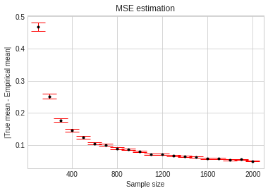
(a) $\Sigma_{1}$

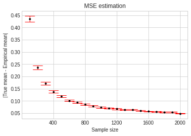
(b) $\Sigma_{2}$

(c) $\Sigma_{3}$

Figure 2: Estimation error as a function of sample size with three different covariance matrices. The bars in the plot show standard error averaged over $1000$ independent replications.

In this section, we describe the numerical experiments on three synthetic problems corresponding to three different covariance matrices $\Sigma_{1},\Sigma_{2}$ and $\Sigma_{3}$, respectively. Both covariance matrices are for a setting with $20$ arms that are jointly Gaussian with mean zero.

These covariance matrices are specified below.

$$\Sigma_{1}=\!\left[\!\begin{array}[]{c c}\mathrm{\mathbf{M}}_{1}&\mathrm{\mathbf{O}}\\ \mathrm{\mathbf{O}}&\mathrm{\mathbf{I}}_{16\times 16}\end{array}\!\right],\Sigma_{2}=\!\left[\!\begin{array}[]{c c}\mathrm{\mathbf{M}}_{1}&\mathrm{\mathbf{O}}\\ \mathrm{\mathbf{O}}&\mathrm{\mathbf{Tr}}_{16\times 16}\end{array}\!\right]\textrm{ and }\Sigma_{3}=\!\left[\!\begin{array}[]{c c}\mathrm{\mathbf{M}}_{2}&\mathrm{\mathbf{O}}\\ \mathrm{\mathbf{O}}&\mathrm{\mathbf{I}}_{16\times 16}\end{array}\!\right],$$ (48)

where $\mathrm{\mathbf{M}}_{1}=\begin{bmatrix}1&0.9&0.9&0.9\\ 0.9&1&0.85&0.85\\ 0.9&0.85&1&0.85\\ 0.9&0.85&0.85&1\end{bmatrix}$, $\mathrm{\mathbf{M}}_{2}=\begin{bmatrix}1&0.5&0.45&0.5\\ 0.5&1&0.45&0.4\\ 0.45&0.45&1&0.4\\ 0.5&0.4&0.4&1\end{bmatrix}$, and $\mathrm{\mathbf{Tr}}_{16\times 16}$ is a tridiagonal matrix with ones along the main diagonal and $0.2$ below and above the diagonal and zeros elsewhere.

The first covariance matrix $\Sigma_{1}$ corresponds to a setting where the first four arms are strongly correlated, while the remaining ones form an independent cluster. On the other hand, the second covariance matrix $\Sigma_{2}$ has a weakly-correlated set of $16$ arms, with the first four arms strongly correlated as in $\Sigma_{1}$. The covariance matrix $\Sigma_{3}$ is a variation to $\Sigma_{1}$, with the correlation between the first four arms weaker than that in $\Sigma_{1}$.

We perform two experiments to study the performance of our MSE estimate, and the successive elimination algorithm in a bandit setting. In the MSE estimation experiments, we use the estimation error as the performance metric, and in the bandit experiment, we use the empirical probability of error as the performance metric. In both settings, we aim to find the best $5$-subset, i.e., the parameter $m=5$. Figures 2(a) , 2(b) and 2(c) present the estimation errors as a function of the sample size for the case of distributions with covariance matrices $\Sigma_{1}$ and $\Sigma_{2}$, respectively. Table 1 presents the MSE-estimation results obtained for the two distributions. For the sake of estimation, $2000$ i.i.d. samples are used in each case, and the standard error is calculated from $1000$ independent replications.

Table 1: The estimation error, i.e., the difference between true and empirical MSE, for three different distributions governed by covariance matrices $\Sigma_{1}$, $\Sigma_{2}$ and $\Sigma_{3}$, respectively. For estimation, $2000$ i.i.d. samples are used, and the standard error is over $1000$ independent replications. The true MSE is calculated using (1), while the empirical MSE is based on (10).

Distribution	True-MSE	Empirical-MSE
$\Sigma_{1}$	15.0	14.91 $\pm 0.002$
$\Sigma_{2}$	14.96	14.97 $\pm 0.002$
$\Sigma_{3}$	15.0	14.99 $\pm 0.002$

The MSE estimation error, i.e., the difference between the true and empirical MSE, is calculated on sample sizes ranging from $100$ to $2000$ for the plots in Figures 2(a), 2(b) and 2(c). The true MSE is calculated using (1), while the empirical MSE is calculated using the expression in (10). From the results in Figures 2(a)–2(c), it is apparent that our proposed MSE estimate is converging rapidly to the true MSE for both distributions.

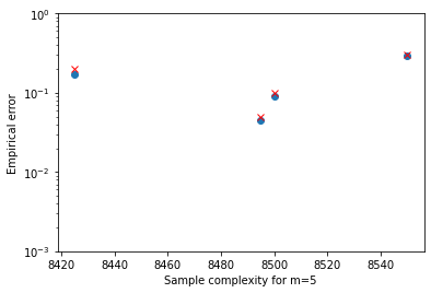
(a) $\Sigma_{1}$

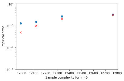
(b) $\Sigma_{2}$

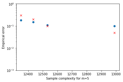
(c) $\Sigma_{3}$

Figure 3: Plots showing the empirical probability of error denoted by circles (’O’) and the specified maximal error probability $\delta$ denoted by crosses (’X’) as a function of the number of samples for the correlated bandit problem with three different covariance matrices.

We now describe the bandit experiment. In the first and third setting, there are $1820$ subsets having the least MSE. The best $5$ subsets in both these settings involves arm $1$ from the first cluster of $4$ arms (in both $M_{1}\textrm{ and }M_{2}$, arm $1$ is the most correlated arm) and any $4$ arms from the other cluster having independent arms. In the second setting, there are $279$ subsets having the least MSE. The best $5$ subset in this setting again involves arm $1$ from the first cluster and $4$ arms from the other cluster.

Figures 3(a), 3(b) and 3(c) plot both the empirical probability of error and the specified maximal error probability $\delta$ of the successive elimination algorithm for four different confidence levels, i.e., $\{0.05,0.1,0.2,0.3\}$ with covariance matrices $\Sigma_{1},\Sigma_{2},\Sigma_{3}$, respectively. In the implementation of successive elimination, we have drawn $1000$ samples in the initialization phase to estimate the covariance matrix. We observed that a short initialization phase led to elimination of many potential best subsets, and to overcome this problem, we draw the $1000$ samples initially.

9 Conclusions

For the problem of estimation of the MSE of a given subset, with a multivariate Gaussian model, we proposed a natural estimator, and derived tail bounds that exponentially concentrate. Next, we framed the estimation problem with bandit feedback in the best-subset identification setting, and proposed a variant of the successive elimination technique. Finally, we also derived a minimax lower bound to understand the fundamental limit on the sample complexity of the aforementioned estimation problem with bandit feedback.

References

• Boda and Prashanth (2019) Boda, V.P., Prashanth, L.A., 2019. Correlated bandits or: How to minimize mean-squared error online, in: International Conference on Machine Learning, PMLR. pp. 686–694.
• Cai et al. (2010) Cai, T.T., Zhang, C.H., Zhou, H.H., 2010. Optimal rates of convergence for covariance matrix estimation. The Annals of Statistics 38, 2118–2144.
• Erraqabi et al. (2017) Erraqabi, A., Lazaric, A., Valko, M., Brunskill, E., Liu, Y., 2017. Trading off rewards and errors in multi-armed bandits, in: International Conference on Artificial Intelligence and Statistics, PMLR. pp. 709–717.
• Even-Dar et al. (2002) Even-Dar, E., Mannor, S., Mansour, Y., 2002. Pac bounds for multi-armed bandit and markov decision processes, in: International Conference on Computational Learning Theory, Springer. pp. 255–270.
• Guestrin et al. (2005) Guestrin, C., Krause, A., Singh, A.P., 2005. Near-optimal sensor placements in gaussian processes, in: International conference on Machine learning, pp. 265–272.
• Gupta et al. (2020) Gupta, S., Joshi, G., Yağan, O., 2020. Correlated multi-armed bandits with a latent random source, in: IEEE International Conference on Acoustics, Speech and Signal Processing (ICASSP), IEEE. pp. 3572–3576.
• Hajek (2009) Hajek, B., 2009. Notes for ECE 534: an exploration of random processes for engineers. Univ. of Illinois at Urbana–Champaign .
• Kaufmann et al. (2015) Kaufmann, E., Cappé, O., Garivier, A., 2015. On the complexity of best arm identification in multi-armed bandit models. The Journal of Machine Learning Research .
• Krause et al. (2008) Krause, A., Leskovec, J., Guestrin, C., VanBriesen, J., Faloutsos, C., 2008. Efficient Sensor Placement Optimization for Securing Large Water Distribution Networks. Journal of Water Resources Planning and Management 134, 516–526.
• Lattimore and Szepesvári (2020) Lattimore, T., Szepesvári, C., 2020. Bandit algorithms. Cambridge University Press.
• Liu and Bubeck (2014) Liu, C.Y., Bubeck, S., 2014. Most correlated arms identification, in: Confernce on Learning Theory, pp. 623–637.
• Paul et al. (2014) Paul, U., Ortiz, L., Das, S.R., Fusco, G., Buddhikot, M.M., 2014. Learning probabilistic models of cellular network traffic with applications to resource management, in: IEEE International Symposium on Dynamic Spectrum Access Networks, pp. 82–91.
• Rigollet and Hütter (2019) Rigollet, P., Hütter, J., 2019. High dimensional statistics. Lecture notes for course 18S997 .
• Sen et al. (2023) Sen, D., Prashanth, L., Gopalan, A., 2023. Adaptive estimation of random vectors with bandit feedback, in: Indian Control Conference, pp. 1–2.
• Wainwright (2019) Wainwright, M.J., 2019. High-dimensional statistics: A non-asymptotic viewpoint. Cambridge University Press.