Ternary and Binary Quantization for Improved Classification

Abstract

Dimension reduction and data quantization are two important methods for reducing data complexity. In the paper, we study the methodology of first reducing data dimension by random projection and then quantizing the projections to ternary or binary codes, which has been widely applied in classification. Usually, the quantization will seriously degrade the accuracy of classification due to high quantization errors. Interestingly, however, we observe that the quantization could provide comparable and often superior accuracy, as the data to be quantized are sparse features generated with common filters. Furthermore, this quantization property could be maintained in the random projections of sparse features, if both the features and random projection matrices are sufficiently sparse. By conducting extensive experiments, we validate and analyze this intriguing property.

I Introduction

Large-scale classification poses great challenges to data storage and computation. To alleviate the problem, a general solution is to reduce data complexity by dimension reduction and quantization. In the paper, we study the methodology of first reducing data dimension by random projection and then quantizing the projections to {0,1}-binary or $\{0,\pm 1\}$-ternary codes. Random projection is implemented by multiplying the data with random matrices [1, 2, 3], and quantization is realized by zeroing out the elements of small magnitude and unifying the elements of large magnitude.

The extreme quantization to binary or ternary codes has been widely applied in large-scale retrieval [4, 5, 6, 7, 8, 9, 10], where the retrieval accuracy usually exhibits obvious degradation due to high quantization errors. In the paper, however, we demonstrate that the quantization could achieve comparable and even higher accuracy for common sparse features, such as the ones generated by discrete wavelet transform (DWT) [11], discrete cosine transom (DCT) [12], and convolutional neural networks (CNN) [13, 14]. The performance improvement caused by quantization, simply called quantization gain, could be explained in terms of feature selection. It is noteworthy that the sparse features mentioned above are mainly generated in frequency and/or spatial domains. The small feature elements are usually of high frequencies, mainly caused by noise and edge gradients. The removing of them will help compact intra-class distances [15], thus improving the classification accuracy. Empirically, the discrimination between objects is mainly determined by the distribution of large feature elements over different frequency and/or spacial components, while insensitive to the energy of each component. For this reason, the magnitude unification of large elements will not cause serious accuracy degradation, and oftentimes it could even raise the accuracy thanks to suppressing underlying outliers.

Moreover, it is observed that the quantization gain could be obtained in the random projections of sparse features, as both the data features and random matrices are sufficiently sparse, such that the projections are sparse. The sparse projections approximately inherit the sparse structure of the original sparse feature and thus can provide similar quantization gains. To generate sparse projections, we suggest to use extremely sparse $\{0,\pm 1\}$-matrices [16, 17] for random projection, such as the ones with only one nonzero element per column, which could provide desired optimization gains. In contrast, another popular random projection matrices, Gaussian matrices [18] can hardly obtain such gains, due to always generating Gaussian-like dense projections.

Here we mainly evaluate the classification performance with the exemplar-based classifiers [19, 20, 21, 22], also known as the instance [23] or nearest neighbor-based classifiers [24], which have been widely recognized as the most biologically-plausible cognitive method [21]. The method categorizes a novel object by comparing its similarity to the exemplars previously stored by class, and could achieve the Bayes-optimal performance, as the exemplars are sampled densely [24]. There are two major ways to measure the similarity to each class. One is to evaluate the distribution of a few most similar exemplars across all classes, such as the known $k$ nearest neighbors ($k$NN) classifier [25], and the other is to calculate the Euclidean distance to the subspace of each class, such as the local subspace classifier (LSC) [26] and its variants [27, 28, 29, 30, 31, 32]. It is easy to see that $k$NN has much lower complexity than LSC, but often suffers inferior performance.

To achieve a balance between them, we propose a simplified variant of LSC, named $k$ nearest exemplar-based classifier ($k$NEC), which measures the similarity to each class by simply summing the distances to $k$ nearest exemplars in the class. Despite the simplicity, $k$NEC often could achieve comparable or better performance than LSC. In fact, the distance summing method adopted in $k$NEC has been early proposed in [33], which however considers the sum of all rather than a few exemplars. The slight modification of $k$NEC could provide significant performance gains, mainly because in practice a query object is often similar to a few rather than all exemplars in its category. The results mentioned above are validated by conducting extensive classification experiments on three benchmark image datasets, including YaleB [34], Cifar10 [35] and ImageNet [36].

II Method

In this section, we describe the pipeline of sparse features generation, projection, quantization and classification.

II-A Sparse feature generation

To obtain relatively good and meaningful classification performance, we suggest to select sparse feature generators in terms of data complexity. For simple datasets, like YaleB, we can simply use linear filters, such as DWT and DCT; and otherwise, we need more sophisticated filters, like convolutional neural networks [13, 14], for more complex datasets, such as Cifar10 and ImageNet. These features capture the characteristics of original images in frequency and/or spacial domains, which as shown in Figure 1, tend to present heavy-tailed symmetric distributions [37, 38, 39]. Usually, the distribution with sharper peak and longer tails means a more sparse structure. By the feature distributions illustrated in Figure 1, we can rank the feature sparsity of three datasets in descending order: YaleB, ImageNet and Cifar10. Interestingly, as will be seen later, the data feature of higher sparsity seems more likely to induce quantization gains.

II-B Sparse matrices-based random projection

For a sparse feature vector $\bm{x}\in\mathbb{R}^{n}$, its random projection is derived by $\bm{y}=\bm{R}\bm{x}$, where $\bm{R}\in\mathbb{R}^{m\times n}$ denotes a random matrix, $m\ll n$. As stated before, like sparse features $x$, sparse projections $y$ tend to provide quantization gains. To generate sparse projections $\bm{y}$, by [40, Sec.2.3], we propose to employ sparse ternary matrices $\bm{R}\in\{0,\pm 1\}^{m\times n}$. Empirically, the quantization gain tends to first increase and then decrease, as the matrix becomes more and more sparse. The latter decreasing trend is incurred by the increasing loss of important features. Empirically, we could obtain a good quantization performance when assigning only one nonzero element in each matrix column. For comparison, we also test Gaussian matrices-based random projections, which always have dense projections and can hardly provide quantization gains.

II-C Ternary and binary quantization

Given a sparse feature $x$ which has been centralized by mean subtraction, we propose to generate the ternary codes by $z_{i}=sign(x_{i})$, if $|x_{i}|>\tau$ and otherwise, $z_{i}=0$. Then, the binary codes are generated by zeroing out all negative entries in the ternary codes. With the same methods, we could generate the codes for random projections $y$. To evaluate the influence of code sparsity, we define by $k/n$ the sparsity ratio of $n$-dimensional ternary code, where $k$ counts the number of nonzeros in the code. Accordingly, the sparsity ratio of binary codes should be about $k/2n$.

II-D Exemplar-based classification

The classification is realized with the proposed $k$NEC, which as stated before, measures the similarity of a query object to each class with the sum of the correlations to $k$-nearest neighbors in the class. Empirically, $k$NEC performs consistently better than $k$NN, and performs comparably or even better than LSC. The reason is as follows. Compared to $k$NN that considers only $k$ nearest exemplars among all classes, $k$NEC involves more exemplars, i.e. $k$ exemplars each class, thus more robust to noise and outlier. As for LSC, it measures the similarity to each class with the Euclidean distance to the subspace spanned by $k$ nearest exemplars in the class. The distance needs to be computed with the minimum square method, while the method inclines to enforcing the $k$ exemplars to contribute equally in representing the query object. However, the constraint is not reasonable, if the similarity of the query object to $k$ exemplars differs widely. In this case, a survey on the distance to each individual exemplar, as done in $k$NEC, should be more reasonable.

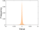
(a) YaleB

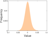
(b) Cifar10

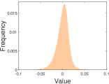
(c) ImageNet

Figure 1: The frequency histograms of the sparse features of YaleB, Cifar10, and ImageNet, which are generated respectively by DCT, AlexNet Conv5 and VGG16 Conv$5\_3$.

III Experiments

	Sparsity ratio	$k/n$	0.1	0.2	0.3	0.4	0.5	0.6	0.7	0.8	0.9	1.0
YaleB	$k$NEC	RC	95.63	96.96	97.44	97.52	97.61	97.73	97.76	97.78	97.78	97.76
		TC	99.77	99.93	99.96	99.99	100.00	100.00	99.98	100.00	99.96	99.96
		BC	99.36	99.78	99.74	99.83	99.87	99.94	99.96	99.98	99.94	99.96
	$k$NN	RC	93.41	94.92	95.37	95.71	95.69	95.74	95.79	95.81	95.79	95.79
		TC	98.90	99.56	99.77	99.82	99.94	99.94	99.86	99.87	99.96	99.86
		BC	97.69	99.12	99.23	99.60	99.74	99.75	99.78	99.92	99.86	99.86
	LSC	RC	98.89	99.15	99.18	99.21	99.24	99.24	99.20	99.20	99.19	99.20
		TC	99.81	99.96	99.96	100.00	100.00	100.00	100.00	100.00	99.96	99.98
		BC	99.58	99.88	99.91	99.95	99.97	99.95	99.94	99.95	99.91	99.94
	SVM	RC	85.03	90.66	92.12	92.77	93.24	93.41	93.64	93.68	93.67	93.67
		TC	99.18	99.82	99.93	99.96	99.94	99.94	99.96	99.95	99.96	99.94
		BC	98.68	99.69	99.84	99.93	99.92	99.92	99.90	99.90	99.94	99.94
Cifar10	$k$NEC	RC	72.39	74.70	75.46	76.16	76.57	76.79	76.61	76.67	76.66	76.71
		TC	72.48	74.81	75.59	76.02	75.93	75.76	75.80	75.42	75.58	75.08
		BC	72.99	75.15	75.82	75.96	76.16	76.06	75.82	75.31	75.38	75.10
	$k$NN	RC	69.21	71.56	72.36	72.88	73.69	73.69	73.83	73.83	73.86	73.78
		TC	68.24	71.33	72.73	72.71	72.66	72.57	72.89	72.43	72.53	71.80
		BC	68.53	71.08	72.66	73.18	73.25	72.94	72.84	72.53	72.16	71.80
	LSC	RC	74.42	76.46	77.28	77.74	78.05	77.98	78.18	78.12	78.20	78.12
		TC	74.70	76.58	77.50	77.87	78.06	77.65	77.88	77.65	77.31	77.35
		BC	74.26	76.90	77.26	77.01	76.94	76.79	77.02	76.13	76.09	75.92
	SVM	RC	77.65	79.24	79.77	80.00	80.09	80.37	80.58	80.52	80.56	80.66
		TC	72.28	74.74	74.92	75.41	75.70	76.10	76.42	75.61	75.09	74.44
		BC	71.94	74.24	74.37	74.95	75.15	74.52	74.36	73.54	73.90	74.36
ImageNet	$k$NEC	RC	39.05	40.73	41.79	42.32	42.61	42.64	42.71	42.70	42.50	42.31
		TC	42.26	42.20	41.43	40.20	38.84	37.54	36.19	35.24	34.28	33.74
		BC	48.28	45.25	42.61	40.55	38.67	37.13	36.01	35.19	34.39	33.74
	$k$NN	RC	36.69	38.49	39.26	39.68	39.95	39.97	40.02	39.93	39.78	39.65
		TC	39.74	39.70	38.77	37.53	36.16	34.64	33.52	32.33	31.48	31.00
		BC	46.07	42.76	40.01	37.80	35.81	34.30	33.27	32.42	31.58	31.00

Table I: Classification accuracy of four classifiers on real-valued codes (RC), ternary codes (TC) and binary codes (BC) across varying sparsity ratio $k/n$. The codes are generated with the sparse features of three different datasets. The best results are highlighted in bold and the second best are underlined.

In this section, we evaluate the quantization performance for the sparse features of YaleB [34], CIFAR10 [35] and ImageNet [36], which are generated respectively by DCT, AlexNet Conv5 and VGG16 Conv$5\_3$ [41], with vectorized dimensions 32256, 43264 and 100352. To reduce simulation time, we further downsample the features to 1200, 4327, and 5018 dimensions. This may cause accuracy degradation but will not influence our comparative studies. The experimental settings are briefly introduced as follows. YaleB contains 2414 frontal-face images with size $192\times 168$ over 38 subjects and about 64 images per subject. We randomly select 9/10 of samples for training and the rest for testing. Considering the DCT and DWT features of YaleB present similar performance, we only present the results of DCT due to limited space. Cifar10 consists of $32\times 32$ natural color images in 10 classes, with 50k samples for training and 10k samples for testing. The same data division is adopted in our experiments. ImageNet contains 1000 classes of images with average resolution $469\times 387$, which has about 1.2M samples for training, 50k samples for validation, and 100k samples for testing. Here we take the validation set for testing since its labels are available.

For comparison, besides the proposed $k$NEC, we also test three other popular classifiers, $k$NN [25], LSC [26], and SVM [42]. For $k$NEC, LSC and $k$NN, we need to previously determine the number $k$ of the nearest neighbors in each class ($k$NEC, LSC) or among all classes ($k$NN). Empirically, it suffices to achieve a good performance when simply setting $k=3$ or 5. Note that we do not test LSC and SVM for ImageNet, due to prohibitive computation. In the following, we evaluate the quantization performance respectively for sparse features and their random projections.

	Sparsity ratio	$k/n$	0.1	0.2	0.3	0.4	0.5	0.6	0.7	0.8	0.9	1.0
YaleB	Sparse Matrix	RC	96.15	97.02	97.27	97.36	97.45	97.51	97.53	97.54	97.53	97.53
		TC	99.64	99.89	99.93	99.91	99.94	99.94	99.92	99.93	99.92	99.91
		BC	98.50	99.47	99.65	99.69	99.64	99.73	99.70	99.74	99.75	99.74
	Gaussian Matrix	RC	95.85	96.90	97.22	97.43	97.45	97.49	97.53	97.55	97.54	97.53
		TC	93.67	95.20	95.74	95.96	95.96	96.10	95.96	95.97	96.14	96.18
		BC	88.96	91.00	92.10	92.52	92.48	92.46	92.50	92.52	92.68	92.82
Cifar10	Sparse Matrix	RC	71.64	74.11	75.07	75.63	75.95	76.12	76.21	76.24	76.28	76.29
		TC	70.79	73.01	74.09	74.69	74.86	75.23	75.31	75.39	75.41	75.48
		BC	67.25	70.50	72.31	72.32	72.68	72.81	73.20	73.20	73.21	73.25
	Gaussian Matrix	RC	70.52	72.97	74.09	74.63	75.05	75.34	75.38	75.46	75.54	75.52
		TC	69.26	71.77	72.99	73.72	74.11	74.35	74.55	74.59	74.64	74.58
		BC	66.02	68.61	69.82	70.92	71.56	72.01	72.34	72.39	72.45	72.41
ImageNet	Sparse Matrix	RC	38.54	40.35	41.28	41.86	42.05	42.08	42.16	42.07	41.94	41.78
		TC	40.70	40.79	40.42	40.33	40.36	40.24	40.09	39.92	39.79	39.51
		BC	36.19	36.12	37.18	37.13	37.20	37.27	37.14	36.92	36.68	36.39
	Gaussian Matrix	RC	37.82	39.61	40.76	41.17	41.47	41.51	41.56	41.50	41.40	41.27
		TC	37.26	39.01	39.96	40.42	40.85	40.94	40.99	41.01	40.78	40.61
		BC	35.18	36.88	38.03	38.41	38.75	38.99	39.09	39.04	39.07	38.80

Table II: Classification accuracy of $k$NEC on real-valued codes (RC), ternary codes (TC) and binary codes (BC) across varying sparsity ratio $k/n$. The codes are generated with the random projections of sparse features over sparse ternary matrices and Gaussian matrices. The projection matrices have compression ratio $m/n=1/2$. The best results are highlighted in bold and the second best are underlined.

III-A Quantization of sparse features

In this part, we aim to prove two facts: 1) the two steps involved in our ternary quantization, namely the removing of small elements and the magnitude unification of large elements, could improve the classification accuracy of sparse features; 2) the proposed $k$NEC could achieve better performance than $k$NN and comparable performance with LSC. To this end, besides ternary codes (TC) and binary codes (BC), we also consider a kind of real-valued codes (RC), which has the same sparsity with TC but has the nonzero values un-quantized. This means that RC will be identical to the original sparse features, when the sparsity ratio $k/n=1$. Note the lower sparsity ratio means higher sparsity.

The results are shown in Table I. It is seen that in three datasets, the performance of RC tends to first increase and then decrease with the sparsity ratio $k/n$ decreasing from 1 to 0.1. The initial increasing trend suggests that the removing of small elements indeed could provide performance gains, while the latter decreasing is incurred by the increasing loss of significant feature elements. Comparing the performance of RC and TC, we can see that TC performs better at low sparsity ratios $k/n\leq 0.3$ both in Cifar10 and ImageNet, and consistently better in YaleB. The performance advantage of TC over RC suggests that the magnitude unification of large elements involved in TC indeed could improve the classification accuracy. Compared to TC, BC discard about half of the features (the negative part) but only suffer from about 0.5% accuracy loss in most cases. The similarity between them implies that the positive and negative parts of sparse features may share similar features. This is indirectly confirmed by the symmetric distributions of sparse features, as illustrated in Figure 1. In ImageNet, BC even outperform TC at $k/n\leq 0.4$. This may be explained by the fact that the sparse features with mean substraction are not exactly symmetric about zero, and it is imperfect to generate TC using the same threshold $\tau$ in both sides.

As for the classifiers, Table I shows that $k$NEC consistently outperforms $k$NN, and performs comparably or better than LSC, with gaps around 1%. In YaleB, $k$NEC even outperforms SVM. The superiority should be attributed to the high similarity between intra-class face samples, which is favorable for exemplar-based classification. In three datasets, three exemplar-based classifiers all could achieve quantization gains, while SVM fails in Cifar10. Furthermore, it is noteworthy that $k$NEC and LSC tend to outperform SVM, when all of them use ternary or binary codes. This suggests that the quantization may be more matched with exemplar-based classification than with SVM. The perfect match between sparse codes and exemplar-based classification may be attributed to its biological plausibility in visual feature extraction [43, 44, 45, 46] and recognition [21].

For the thee datasets, by their capability of inducing optimization gains as shown in Table I, we can rank them in descending order: YaleB, ImageNet and Cifar10. Interestingly, the order happens to agree with the feature sparsity order we have ranked with the feature distributions shown in Figure 1. As stated in Section II-A, this implies that the features with higher sparsity, namely the ones with sharper peaks and longer tails, are more prone to providing quantization gains.

Finally, it is noteworthy $k$NEC could achieve comparable or even better classification performance than deep networks, if exploiting sparse features from deeper network layers. For instance, using the output features of the penultimate, fully-connected layer, for Cifar10 with classification accuracy 89.02% on AlexNet, we obtain the $k$NEC accuracy of 89.66%, 89.52% and 89.50% respectively for RC, TC and BC all with sparsity ratio $k/n=10\%$; and for ImageNet with classification accuracy 65.76% on VGG16, $k$NEC achieves the accuracy of 65.54%, 65.17% and 65.24% for the above-mentioned three codes with $k/n=30\%$.

III-B Quantization of sparse random projections

We now move on to prove that the quantization gain could also be obtained for the random projections of sparse features, if both the features and random projection matrices are sufficiently sparse, such that the projections are sparse. For this purpose, we test the sparse features with varying sparsity ratio $k/n$, and implement random projections with a kind of extremely sparse random matrices $\bm{R}\in\{0,\pm 1\}^{m\times n}$, which has only one nonzero entry per column. For comparison, we also test Gaussian matrices based random projections, which always have dense distributions. To obtain relatively stable classification results [1], we obtain an average result in each trial by repeating 5 times random projections.

The results are provided in Table II. It is seen that sparse matrices achieve quantization gains with TC both in YaleB ($k/n\leq 1$) and ImageNet ($k/n\leq 0.2$). As to why the gain is not obtained in Cifar10, it may be because its features have relatively weak sparsity nature compared to the features of other two datasets, as illustrated in Figure 1. As demonstrated before, the problem should be addressed if we explore deeper networks to generate more abstract and sparse features for Cifar10. As for Gaussian matrices, it is seen that the best performance is always obtained by RC, rather than by TC or BC. This suggests that Gaussian matrices can hardly offer quantization gains due to holding dense projections. Furthermore, it is noteworthy that the RC performance of Gaussian matrices is always inferior to the TC performance of sparse matrices. This encourages us to exploit sparse matrices instead of Gaussian matrices for quantization, both in terms of performance and complexity.

IV Conclusion and Discussion

For sparse features or their sparse random projections, we have shown that ternary quantization on them could improve classification performance, and binary quantization could provide competitive performance. The intriguing quantization performance can be explained with feature selection: the zero out of small elements helps reduce noise and compact intra-class distances, while the magnitude unification of large elements helps remove underlying outliers. Interestingly, the quantization tends to provide better classification performance when combined with exemplar-based classifiers, than with other types of classifiers, such as SVM. The perfect match between sparse codes and exemplar-based classifiers may be explained by its biological plausibility: it has been found that the human vision system captures visual features with Gabor-like sparse binary codes [43, 44, 45, 46], and recognizes them with exemplar-based cognitive mechanism [21]. Finally, it is noteworthy that in our classification both the initial random projection of sparse features and the following exemplar-based classification are linear projection models. Essentially, the cascade of the two models forms a three-layer neural network, with ternary/binary parameters/activations. Usually, such kind of quantization networks performs comparably or even better than its full-precision counterparts [47], while the mechanism behind the intriguing performance remains unclear. Our work sheds light on the problem.

References

- [1] E. Bingham and H. Mannila, “Random projection in dimensionality reduction: applications to image and text data,” in Proceedings of the 7th ACM SIGKDD International Conference on Knowledge Discovery and Data Mining, pp. 245–250, 2001.
- [2] D. Fradkin and D. Madigan, “Experiments with random projections for machine learning,” in Proceedings of the 9th ACM SIGKDD international conference on Knowledge discovery and data mining, 2003.
- [3] X. Z. Fern and C. E. Brodley, “Random projection for high dimensional data clustering: A cluster ensemble approach,” in Proceedings of the Twentieth International Conference on International Conference on Machine Learning, 2003.
- [4] P. Indyk and R. Motwani, “Approximate nearest neighbors: towards removing the curse of dimensionality,” in Proceedings of the thirtieth annual ACM symposium on Theory of computing, 1998, pp. 604–613.
- [5] M. S. Charikar, “Similarity estimation techniques from rounding algorithms,” in Proceedings of the thiry-fourth annual ACM symposium on Theory of computing, 2002, pp. 380–388.
- [6] M. Li, S. Rane, and P. Boufounos, “Quantized embeddings of scale-invariant image features for mobile augmented reality,” in 2012 IEEE 14th International Workshop on Multimedia Signal Processing (MMSP). IEEE, 2012, pp. 1–6.
- [7] P. Li, M. Mitzenmacher, and A. Shrivastava, “Coding for random projections,” in International Conference on Machine Learning. PMLR, 2014, pp. 676–684.
- [8] P. Li, M. Mitzenmacher, and M. Slawski, “Quantized random projections and non-linear estimation of cosine similarity,” in Advances in Neural Information Processing Systems, 2016, pp. 2756–2764.
- [9] C. Liu, L. Fan, K. W. Ng, Y. Jin, C. Ju, T. Zhang, C. S. Chan, and Q. Yang, “Ternary hashing,” arXiv preprint arXiv:2103.09173, 2021.
- [10] M. Chen, W. Li, and W. Lu, “Deep learning to ternary hash codes by continuation,” Electronics Letters, vol. 57, no. 24, pp. 925–926, 2021.
- [11] S. Mallat, A Wavelet Tour of Signal Processing, Third Edition: The Sparse Way, 3rd ed. Orlando, FL, USA: Academic Press, Inc., 2009.
- [12] R. C. Gonzalez and R. E. Woods, Digital Image Processing (3rd Edition). USA: Prentice-Hall, Inc., 2006.
- [13] A. Sharif Razavian, H. Azizpour, J. Sullivan, and S. Carlsson, “CNN features off-the-shelf: an astounding baseline for recognition,” in Proceedings of the IEEE conference on computer vision and pattern recognition workshops, 2014, pp. 806–813.
- [14] J. Donahue, Y. Jia, O. Vinyals, J. Hoffman, N. Zhang, E. Tzeng, and T. Darrell, “Decaf: A deep convolutional activation feature for generic visual recognition,” in International conference on machine learning. PMLR, 2014, pp. 647–655.
- [15] J. Zarka, L. Thiry, T. Angles, and S. Mallat, “Deep network classification by scattering and homotopy dictionary learning,” in International Conference on Learning Representations, 2020.
- [16] D. Achlioptas, “Database-friendly random projections: Johnson–Lindenstrauss with binary coins,” J. Comput. Syst. Sci., vol. 66, no. 4, pp. 671–687, 2003.
- [17] P. Li, T. J. Hastie, and K. W. Church, “Very sparse random projections,” in Proceedings of the 12th ACM SIGKDD international conference on Knowledge discovery and data mining, 2006.
- [18] S. Dasgupta and A. Gupta, “An elementary proof of a theorem of johnson and lindenstrauss,” Random Structures & Algorithms, vol. 22, no. 1, pp. 60–65, 2003.
- [19] R. M. Nosofsky, “Tests of an exemplar model for relating perceptual classification and recognition memory.” Journal of experimental psychology: human perception and performance, vol. 17, no. 1, p. 3, 1991.
- [20] R. J. Peters, F. Gabbiani, and C. Koch, “Human visual object categorization can be described by models with low memory capacity,” Vision Research, vol. 43, no. 21, pp. 2265–2280, 2003.
- [21] F. G. Ashby and L. Rosedahl, “A neural interpretation of exemplar theory.” Psychological review, vol. 124, no. 4, p. 472, 2017.
- [22] C. R. Bowman, T. Iwashita, and D. Zeithamova, “Tracking prototype and exemplar representations in the brain across learning,” Elife, vol. 9, p. e59360, 2020.
- [23] S. Cost and S. Salzberg, “A weighted nearest neighbor algorithm for learning with symbolic features,” Machine learning, vol. 10, no. 1, pp. 57–78, 1993.
- [24] T. Cover and P. Hart, “Nearest neighbor pattern classification,” IEEE Transactions on Information Theory, vol. 13, no. 1, pp. 21–27, 1967.
- [25] L. E. Peterson, “K-nearest neighbor,” Scholarpedia, vol. 4, no. 2, p. 1883, 2009.
- [26] J. Laaksonen, “Local subspace classifier,” in International Conference on Artificial Neural Networks. Springer, 1997, pp. 637–642.
- [27] I. Naseem, R. Togneri, and M. Bennamoun, “Linear regression for face recognition,” IEEE transactions on pattern analysis and machine intelligence, vol. 32, no. 11, pp. 2106–2112, 2010.
- [28] C. J. Veenman and M. J. Reinders, “The nearest subclass classifier: A compromise between the nearest mean and nearest neighbor classifier,” IEEE Transactions on Pattern Analysis and Machine Intelligence, vol. 27, no. 9, pp. 1417–1429, 2005.
- [29] H. Cevikalp, D. Larlus, M. Douze, and F. Jurie, “Local subspace classifiers: Linear and nonlinear approaches,” in 2007 IEEE Workshop on Machine Learning for Signal Processing. IEEE, 2007, pp. 57–62.
- [30] J. Lu and Y.-P. Tan, “Nearest feature space analysis for classification,” IEEE Signal Processing Letters, vol. 18, no. 1, pp. 55–58, 2010.
- [31] Y. Liu, S. S. Ge, C. Li, and Z. You, “-ns: A classifier by the distance to the nearest subspace,” IEEE Transactions on Neural Networks, vol. 22, no. 8, pp. 1256–1268, 2011.
- [32] Y. G. Wang, “Consistency and convergence rate for nearest subspace classifier,” Information and Inference: A Journal of the IMA, vol. 6, no. 1, pp. 41–57, 2017.
- [33] R. M. Nosofsky, “Exemplar-based accounts of relations between classification, recognition, and typicality.” Journal of Experimental Psychology: learning, memory, and cognition, vol. 14, no. 4, p. 700, 1988.
- [34] K. Lee, J. Ho, and D. Kriegman, “Acquiring linear subspaces for face recognition under variable lighting,” IEEE Trans. PAMI, vol. 27, no. 5, pp. 684–698, 2005.
- [35] A. Krizhevsky and G. Hinton, “Learning multiple layers of features from tiny images,” Master’s thesis, Department of Computer Science, University of Toronto, 2009.
- [36] J. Deng, W. Dong, R. Socher, L.-J. Li, K. Li, and L. Fei-Fei, “ImageNet: A Large-Scale Hierarchical Image Database,” in IEEE Conference on Computer Vision and Pattern Recognition, 2009.
- [37] R. Reininger and J. Gibson, “Distributions of the two-dimensional dct coefficients for images,” IEEE Transactions on Communications, vol. 31, no. 6, pp. 835–839, 1983.
- [38] E. P. Simoncelli, “Modeling the joint statistics of images in the wavelet domain,” in Wavelet Applications in Signal and Image Processing VII, vol. 3813. International Society for Optics and Photonics, 1999, pp. 188–195.
- [39] A. Garriga-Alonso, C. E. Rasmussen, and L. Aitchison, “Deep convolutional networks as shallow gaussian processes,” in International Conference on Learning Representations, 2019.
- [40] S. Kotz, T. Kozubowski, and K. Podgorski, The Laplace distribution and generalizations: a revisit with applications to communications, economics, engineering, and finance. Springer Science & Business Media, 2012.
- [41] K. Simonyan and A. Zisserman, “Very deep convolutional networks for large-scale image recognition,” arXiv preprint arXiv:1409.1556, 2014.
- [42] C. Cortes and V. Vapnik, “Support-vector networks,” Machine learning, vol. 20, no. 3, pp. 273–297, 1995.
- [43] B. Olshausen and D. Field, “Emergence of simple-cell receptive field properties by learning a sparse code for natural images,” Nature, vol. 381, pp. 607–609, April 1996.
- [44] B. A. Olshausen and D. J. Field, “Sparse coding with an overcomplete basis set: A strategy employed by v1?” Vision research, vol. 37, no. 23, pp. 3311–3325, 1997.
- [45] J. H. Van Hateren and A. van der Schaaf, “Independent component filters of natural images compared with simple cells in primary visual cortex,” Proceedings of the Royal Society of London. Series B: Biological Sciences, vol. 265, no. 1394, pp. 359–366, 1998.
- [46] A. Hyvärinen and U. Köster, “Complex cell pooling and the statistics of natural images,” Network: Computation in Neural Systems, vol. 18, no. 2, pp. 81–100, 2007.
- [47] H. Qin, R. Gong, X. Liu, X. Bai, J. Song, and N. Sebe, “Binary neural networks: A survey,” Pattern Recognition, vol. 105, p. 107281, 2020.