The initial state of Pluto-Charon with Tidal Evolution

Abstract

Presently, Pluto and Charon have been in the tidal locking and the ratio of the Pluto and Charon’s spin velocity to the orbital mean motion is 1. In other words, both of them have a 1:1 spin-orbit resonance. We can use the theory of tidal evolution to get this conclusion. Thus, I’d like to test the influence of tidal evolution at Pluto-Charon and test the different initial states that can evolve to the current state. At last, I’d like to describe the evolutionary process in different situations on purpose. At a binary system, the part of liquid at the one is drawn by the other rotating at orbit. We call the part that is drawn as a bulge. Then, the difference between spin and mean motion generates a friction force to reduce the spin velocity to be the same as mean motion. This process is called “tidal evolution” and it has the endpoint like the Pluto-Charon’s current state. In general, we have the $\Delta t$ model and Q model to describe the tidal evolution. $\Delta t$ model and Q model are decided by the lag angle. The lag angle is generated when the spin speed is different from the mean motion. The bulge that is generated by the last moment spins faster than the bulge raising at this moment. Then, the angle between the bulge generated at the last moment and the bulge raising at current is called the lag angle. About the model of tidal evolution, we can find the equation for the $\Delta t$ model and Q model at W. H. Cheng et al. 2014. At the truncation equation, the tidal evolution equation will have an unnecessary overshoot. This result, we will show it at $\Delta t$ model. Thus, I’d like to find a more exact tidal evolution equation for the Q model. Then, I simulated the tidal evolution of Pluto-Charon with both models. At my results, the possible initial states that can evolve to the current state abide by the curve the conservation of angular momentum. This conclusion implies a function that Pluto-Charon’s initial state should abide by instead of the exact value. Then, I added the influence of inclination. However, the simulating result shows the inclination decays quickly. This means the inclination weakly affects the tidal evolution and the current inclination is zero. At last, I discussed the situation that orbital semi-major axis overshoots before coming back to the current value. This situation means the binary will have a high orbital semi-major axis and high eccentricity. This happens at the low relative rate of tidal dissipation since the perturbation that Charon’s spin velocity and eccentricity lead to. In conclusion, I simulated the tidal evolution of Pluto-Charon and found a relation between the initial states. Besides, I showed the fact that we can ignore the influence of inclination and a special state with the high orbital semi-major axis and high eccentricity. This result lets me develop an interest in other binary systems. (If the system is the planet and satellite, the satellite’s influence can be ignored). Then, a system with the low relative rate of tidal dissipation makes this system be provided with high eccentricity and evolve to the tidal locking at the end. This will significantly influence the weather in this system.

1.   Introduction

Between two stars, the tidal evolution will change the orbital semi-major axis $a$, the orbital eccentricity $e$, the spin angular velocities of Pluto $\psi_{p}$, the spin angular velocities of Charon $\psi_{c}$, and the inclination $I$. The end of tidal evolution is the ratio of the binary stars’ spin velocity to mean motion is 1 (Ignore the permanent quadrupole moment). The present state of Pluto and Charon is the end of tidal evolution. Although there are other satellites like Styx, Nix, Hydra, etc, Charon is bigger than the others. Thus, we can ignore the other satellites. Pluto-Charon is suitable for the theory of tidal evolution. However, the barycentre of Pluto and Charon is outside Pluto, so we can’t regard Charon as a satellite to ignore the contribution of Charon at tidal evolution.

I don’t preset the initial values of all parameters the tidal evolution depends. Even the huge orbital semi-major axis and eccentricity at the initial state sounds incredible. Robin M. Canup (2011) shows many possible states in her article Table 2 with smoothed particle hydrodynamic (SPH). Canup shows an intact process to form about Pluto and Charon, etc. Her result implies we should consider the wider initial state.

On the other hand, I don’t consider The permanent quadrupole moment because the spin-Orbit resonance is 1:1. The permanent quadrupole moment will influence the end of tidal evolution like Mercury that the planet is trapped in a 3:2 spin–orbit resonance with the Sun, rather than the expected 1:1 synchronous state.

In the following, I show my simulation to compare W.H. Cheng. On the one hand, it verifies my result to be right. On the other hand, I show that the result is more exact to satisfy the conservation of angular momentum. At last, I will add the inclination at my simulation.

In section 2, we use the $\triangle t$ model for tidal evolution. I confuse the Cheng’s figure that they change the initial eccentricity, but the final orbital semi-major axis is the same. Thus, I repeat simulating the tidal evolution. We have the equation of tidal evolution(P. Hut 1980). I use their equation to simulate the evolution of Pluto-Charon, and I also use the approximate expression derived from Zahn 1977 to compare the evolution to W.H. Cheng. At this section last, I show the curve of many possible initial states which can approach the present state at the end of tidal evolution.

In Section 3, we use the Q model for tidal evolution. At Cheng’s article, the eccentricity e=3 will lead to that orbital semi-major axis overshoots before coming back to the current value. At my section 2, we can see the situation that orbital semi-major axis overshoots at the equation doesn’t including all order of eccentricity. Thus, I attempt to calculate the exact expression of tidal evolution. However, the integral isn’t integrable. Thus, I follow the way(Zahn 1966, Zahn 1977) to calculate more exact tidal evolution to solve the problem of overshooting.

In section 4, we show the model including inclination. (F. Mignard 1979). When the tidal evolution including inclination shows that the inclination is quickly decaying rather than the other parameters. It shows that the inclination of Pluto-Charon is zero accords with the present state, but because it decays very quickly, we can’t find any outstanding change when we consider the inclination. We can’t use this model to argue the value of initial inclination.

Before starting the next section, I show all the parameters we need in table 1.

Table 1: variable table

variable	meaning	note
G	gravitational constant
$\dot{\psi}_{i}$	spin velocity	i=p : Pluto; i=c : Charon
$\alpha_{i}$	spin velocity (mean motion)
$R_{i}$	radius(km)	$R_{p}$:1153; $R_{c}$:606
a	orbital semi-major axis
X	a/$R_{p}$
$M_{i}$	mass(kg)	$M_{p}$:1.304e22 $M_{c}$:1.519e21
$\mu$	reduced mass	$\frac{M_{p}M_{c}}{M_{p}+M_{c}}$
$C_{i}$	the moment of inertia ($Kg\cdot m^{2}$)	$C_{p}$:5.686e33; $C_{c}$:2.232e32
$k_{2i}$	Love number	$k_{2}p$:0.058; $k_{2}c$:0.006
$\triangle t_{i}$	delay time	$\triangle t_{p}$:600
$Q_{i}$	dissipation function	$Q_{p}$:100
I	inclination	$I_{p}=I$ $I_{s}=0$
e	eccentricity
$A_{\triangle t}$	the relative rate of tidal dissipation ($\triangle t$ model)	$\frac{k_{2c}}{k_{2p}}\frac{\triangle t_{c}}{\triangle t_{p}}(\frac{M_{p}}{M_{c}})^{2}(\frac{R_{c}}{R_{p}})^{5}$
$A_{Q}$	the relative rate of tidal dissipation (Q model)	$\frac{k_{2c}}{k_{2p}}\frac{Q_{p}}{Q_{c}}(\frac{M_{p}}{M_{c}})^{2}(\frac{R_{c}}{R_{p}})^{5}$

2.   Tidal evolution with $\Delta t$ model

Now, the Pluto-Charon is at the end of tidal evolution. Thus, we want to consider the tidal interaction at Pluto-Charon. Tidal interaction at Pluto-Charon makes friction. Each star raises tides on the surface of the other. But, the tides with respect to the line joining the centers of two stars. When the star spins faster or slower. The friction from tidal bulge will make a torque decelerates or accelerates the spin. Thus, at last, Pluto and Charon will face each other. It makes them not feel the friction from the tidal force.

First, we showed the equation we used at different order eccentricity. Before the equation, let us show a brief introduction to tidal evolution. The definition of $\triangle t$ and Q is defined from the lag angle between spin velocity and mean motion. Choosing a situation that the spin velocity of the satellite is faster than mean motion. the $\dot{\psi}_{p}>n$. Then, tidal-raising satellite by an angle $\delta$. At $\Delta t$ model, $\Delta t$ is defined by $\delta=(\dot{\psi}_{p}-n)\triangle t$. In Q model, Q is defined by $\sin 2\delta=-Q^{-1}$. From these definitions, if spin velocity equals mean motion, the lag angle is zero. In other words, the tidal friction disappears.

In chapter five of the book ”Dynamics of Close Binary System”, we know a way to derive the equation of tidal evolution. We need to find the perturbation force and substitute them to the Gaussian perturbation equation.

2.1 The influence of different order at eccentricity

First, we followed a result (Eq.3.6$\sim$ Eq.3.8) from Zahn 1977. The equation he constructed was simply to switch between $\triangle t$ model and Q model. However, it is a truncation of the expansion of eccentricity.

$$\frac{1}{n}\frac{d}{dt}(\dot{\psi}_{i})=\frac{3}{2}\frac{GM_{j}^{2}}{C_{i}R_{i}}(\frac{R_{i}}{a})^{6}$$

$$\phantom{\frac{d}{dt}(I\Omega)}\cdot[\epsilon_{2}^{22}+e^{2}(\frac{1}{4}\epsilon_{2}^{12}-5\epsilon_{2}^{22}+\frac{49}{4}\epsilon_{2}^{32})+O(e^{4})]$$ (1)

$$\frac{1}{a}\frac{da}{dt}=-3n\frac{M_{c}}{M_{p}}(\frac{R_{p}}{a})^{5}$$

$$\phantom{\frac{da}{dt}}\cdot[\epsilon_{2}^{22}+e^{2}(\frac{3}{4}\epsilon_{2}^{10}+\frac{1}{8}-5\epsilon_{2}^{22}+\frac{147}{8}\epsilon_{2}^{32})+O(e^{4})]$$ (2)

$$\frac{1}{e}\frac{de}{dt}=-\frac{3}{4}n\frac{M_{c}}{M_{p}}(\frac{R_{p}}{a})^{5}$$

$$\phantom{\frac{de}{dt}}\cdot[\frac{3}{2}\epsilon_{2}^{10}-\frac{1}{4}\epsilon_{2}^{12}-\epsilon_{2}^{22}+\frac{49}{4}\epsilon_{2}^{32}+O(e^{2})]$$ (3)

Here, the $\epsilon_{2}^{lm}$ is defined at Zahn 1977 (Eq 2.7). Let us substitute $\epsilon_{2}^{lm}=k_{2}\triangle t(ln-m\dot{\psi}_{i})$. Here, we ignore the other coefficients $E_{n}$. (Eq 2.8 Zahn 1977). Then, we have the following equation (4)(5)(6). And the figure 1 is the simulation result from these equations.

$$\frac{d\dot{\psi}_{i}}{dt}=-\frac{3G{M_{j}}^{2}}{C_{i}R_{i}}k_{2i}\triangle t_{i}(\frac{R_{i}}{a})^{6}[(1+\frac{15}{2}e^{2})\frac{\psi_{i}}{n}-(1+\frac{27}{2}e^{2}+O(e^{4})]$$ (4)

$$\frac{1}{a}\frac{da}{dt}=\frac{6G}{\mu R_{p}^{3}}k_{2p}\triangle t_{p}{M_{c}}^{2}(\frac{R_{p}}{a})^{8}[(1+\frac{27}{2}e^{2})(\frac{\psi_{p}}{n}+A_{\triangle t}\frac{\psi_{c}}{n})$$

$$\phantom{\frac{dX}{dt}=\frac{6G}{\mu X^{7}}k_{2p}\triangle t_{p}{M_{s}}^{2}(\frac{1}{R_{p}})^{3}+{}}-(1+23e^{2})(1+A_{\triangle t})+O(e^{4})]$$ (5)

$$\frac{1}{e}\frac{de}{dt}=\frac{27G}{\mu R_{p}^{3}}K_{2p}\triangle t_{p}{M_{s}}^{2}(\frac{R_{p}}{a})^{8}[\frac{11}{18}(\frac{\dot{\psi_{p}}}{n}+A_{\triangle}t\frac{\dot{\psi_{s}}}{n})$$

$$\phantom{\frac{de}{dt}=\frac{27eG}{\mu X^{8}}K_{2p}\triangle t_{p}{M_{s}}^{2}(\frac{1}{R_{p}})^{3}}-(1+A_{\triangle}t)+O(e^{2})]$$ (6)

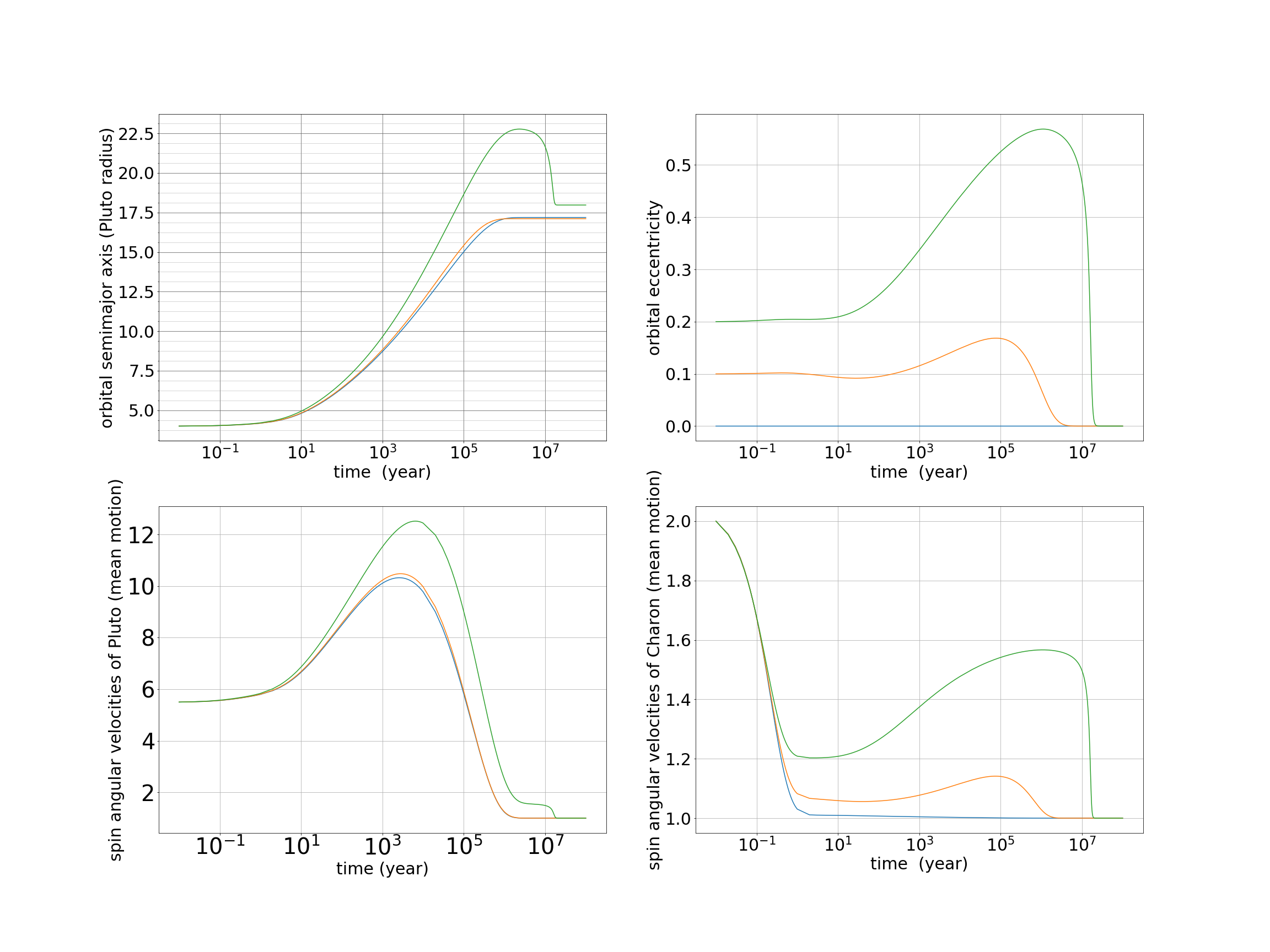
Figure 1: Tidal evolution with $\triangle t$ model follow the equation (4)(5)(6)

At figure 1, I’d like to compare the result with Cheng’s article. I chose the same parameter as Cheng including $A_{\triangle t}$=10 and the same initial state. The initial ratio of the semi-major axis to Pluto’s radius X is 4, the initial ratio of Pluto’s spin velocity to mean motion $\alpha_{p}$ is 5.5, the initial ratio of Charon’s spin velocity to mean motion $\alpha_{c}$ is 2, and the initial eccentricity is 0, 0.1, 0.2, and 0.3.

The figure (1) is my result and it follows the equation (4)(5)(6). This equation just expands to order 2 of eccentricity. When the eccentricity e=0.2, the orbital semi-major axis a will overshoot before coming back to the current value. And when the e=0.3, this evolution can’t converge to a stable value.

Then, we compare this result to figure 2 which is the $\Delta t$ model at Cheng’s article and discuss the problem in figure 1.

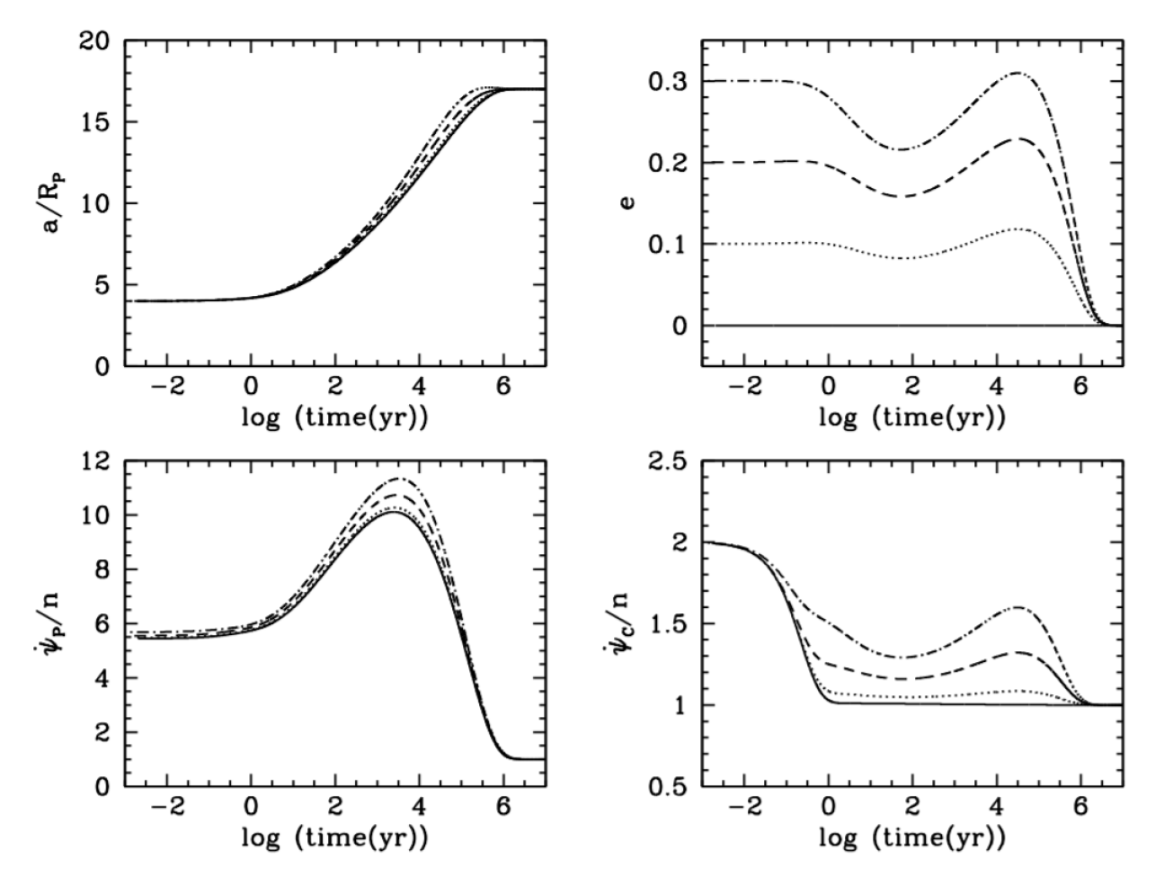
Figure 2: Tidal evolution with $\triangle t$ model from Cheng’s Fig2

Cheng’s figure doesn’t happen that overshoot before coming back to the current value, and his figure also converges when the initial eccentricity e=0.3. However, it is still strange, when he changes the initial eccentricity. The final state doesn’t change. Although Cheng mentions the no conservation of angular momentum since the truncation of the expansion eccentricity. But, this argument is mentioned in his Q model. Thus, I simulated the exact expression of tidal evolution following P. Hut 1980. The equations (7)(8)(9) are from Hut and figure 3 is the simulation result of these equations. Hut’s equation includes all orders of eccentricity. The only inaccuracy part is that the tidal force just includes the $r^{-3}$. However, the perturbation term of $r^{-4}$ isn’t important compared to the influence of eccentricity when we change the initial eccentricity.

$$\frac{1}{n}\frac{d\dot{\psi}_{i}}{dt}=-\frac{3G{M_{j}}^{2}}{C_{i}R_{i}}k_{2i}\triangle t_{i}(\frac{R_{i}}{a})^{6}[f_{1}(e^{2})\frac{\dot{\psi}_{i}}{n}-f_{2}(e^{2})]$$ (7)

$$\frac{1}{a}\frac{da}{dt}=\frac{6G}{\mu R_{p}^{3}}k_{2p}\triangle t_{p}{M_{c}}^{2}(\frac{R_{p}}{a})^{8}[f_{2}(e^{2})(\frac{\dot{\psi}_{p}}{n}+A_{\triangle t}\frac{\dot{\psi}_{c}}{n})$$

$$\phantom{\frac{dX}{dt}=\frac{6G}{\mu X^{7}}k_{2p}\triangle t_{p}{M_{s}}^{2}(\frac{1}{R_{p}})^{3}+{}}-f_{3}(e^{2})(1+A_{\triangle t})]$$ (8)

$$\frac{1}{e}\frac{de}{dt}=\frac{27G}{\mu R_{p}^{3}}k_{2p}\triangle t_{p}{M_{s}}^{2}(\frac{R_{p}}{a})^{8}[f_{4}(e^{2})\frac{11}{18}(\frac{\dot{\psi_{p}}}{n}+A_{\triangle}t\frac{\dot{\psi_{s}}}{n})$$

$$\phantom{\frac{de}{dt}=\frac{27eG}{\mu X^{8}}k_{2p}\triangle t_{p}{M_{s}}^{2}(\frac{1}{R_{p}})^{3}}-f_{5}(e^{2})(1+A_{\triangle}t)]$$ (9)

$$f_{1}(e^{2})=(1+3e^{2}+\frac{3}{8}e^{4})/(1-e^{2})^{9/2}$$

$$f_{2}(e^{2})=(1+\frac{15}{2}e^{2}+\frac{45}{8}e^{4}+\frac{5}{16}e^{6})/(1-e^{2})^{6}$$

$$f_{3}(e^{2})=(1+\frac{31}{2}e^{2}+\frac{255}{8}e^{4}+\frac{185}{16}e^{6}+\frac{25}{64}e^{8})/(1-e^{2})^{15/2}$$

$$f_{4}(e^{2})=(1+\frac{3}{2}e^{2}+\frac{1}{8}e^{4})/(1-e^{2})^{5}$$

$$f_{5}(e^{2})=(1+\frac{15}{4}e^{2}+\frac{15}{8}e^{4}+\frac{5}{64}e^{6})/(1-e^{2})^{13/2}$$

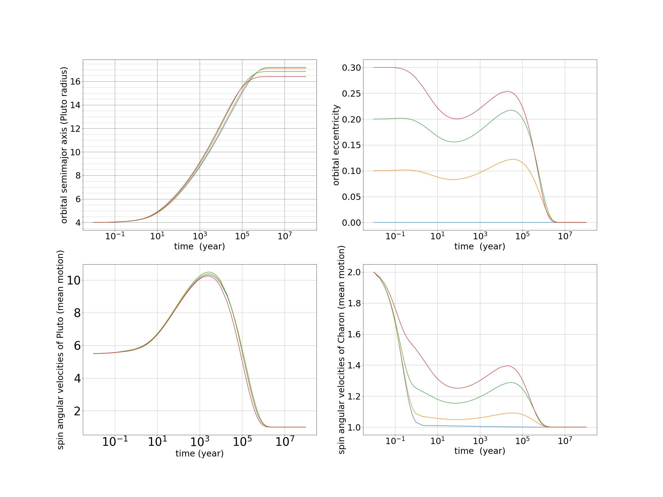
Figure 3: Tidal evolution with $\triangle t$ model follow the equation (7)(8)(9)

The figure 3 satisfies the conservation of angular momentum perfectly and it resolves the problem that orbital semi-major axis overshoot before coming back to the current state. We can see from figure 3. Even we change the eccentricity, it still conserves the angular momentum. At Cheng’s article, the different eccentricity gives the same orbital semi-major axis at the end state. We can see in figure 2.

In this subsection, I show it is different between figure 1 and figure 3. This result will help us to modify the tidal evolution of the Q model. I will discuss this in section 3.

2.2 The possible initial states evolve to the current state

On my purpose, we want to find the initial states which can evolve to the current state and the conservation of angular momentum is the key to find it. Thus, I’d like to check the different initial states that their end point of tidal evolution will be the Pluto-Charon’s current state. Before we test the possible initial states can evolve to the current state, let us check which parameter is important at this evolution. We follow the conservation of angular momentum.

$$\mu\sqrt{G(M_{p}+M_{c})a(1-e^{2})}+C_{p}\frac{G(M_{p}+M_{c})}{a^{3}}\alpha_{p}+C_{c}\frac{G(M_{p}+M_{c})}{a^{3}}\alpha_{c}$$ (10)

The $C_{c}<<C_{p}$, so the $\alpha_{c}$ barely affects the tidal evolution. And the eccentricity $e^{2}$ is very smaller than 1 when eccentricity is 0.1, 0.2, 0.3. Thus, we should find an obvious relation which satisfies the conservation of angular momentum by plotting orbital semi-major axis and Pluto’s spin velocity. Thus, I will input a lot of initial states and leave the points they can evolve the current state. Like the figure 4. Notice these points are tested by equation (7)(8)(9).

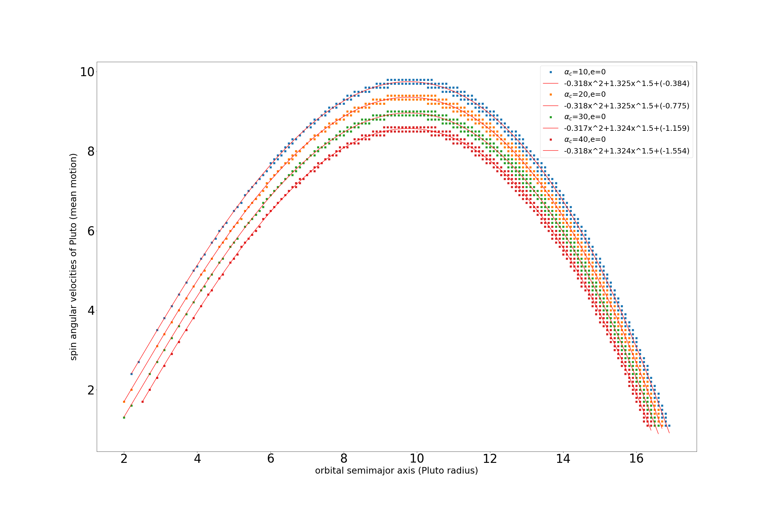
Figure 4: The possible initial state at $\alpha_{c}$=10, 20, 30, and 40 and e=0

At figure 4, the x-axis is an orbital semi-major axis, and the y-axis is the $\alpha_{p}$. At this figure, the eccentricity I set 0.0, and I set different $\alpha_{c}$ 10, 20, 30, and 40 with different colors. The scatter points are that I test the orbital semi-major axis from 1 to 17 Pluto’s radius and Pluto’s spin velocity from 1 to 10 and if they can evolve to the current state (end X is $16.9<X<17.1$). Then, I plot this point in figure 4. The line is the fitting curve. These fitting curves can be derived from the equation of conservation of angular momentum. We use the equation (10) to derive the fitting line.

$$\alpha_{p}=-\frac{\mu}{C_{p}}R_{p}^{2}\sqrt{(1-e^{2})}X^{2}+\frac{\mu\sqrt{17}R_{p}^{2}+C_{c}17^{-1.5}+C_{p}17^{-1.5}}{C_{p}}X^{1.5}-\frac{C_{c}}{C_{p}}\alpha_{c}$$ (11)

Then, let e=0. We substitute the value. Then, we get $\alpha_{p}=-0.318X^{2}+1.327X^{1.5}-0.039\alpha_{c}$. This equation matches the fitting curves at figure 4.

Then, we also show the different initial states by changing the eccentricity at figure 5.

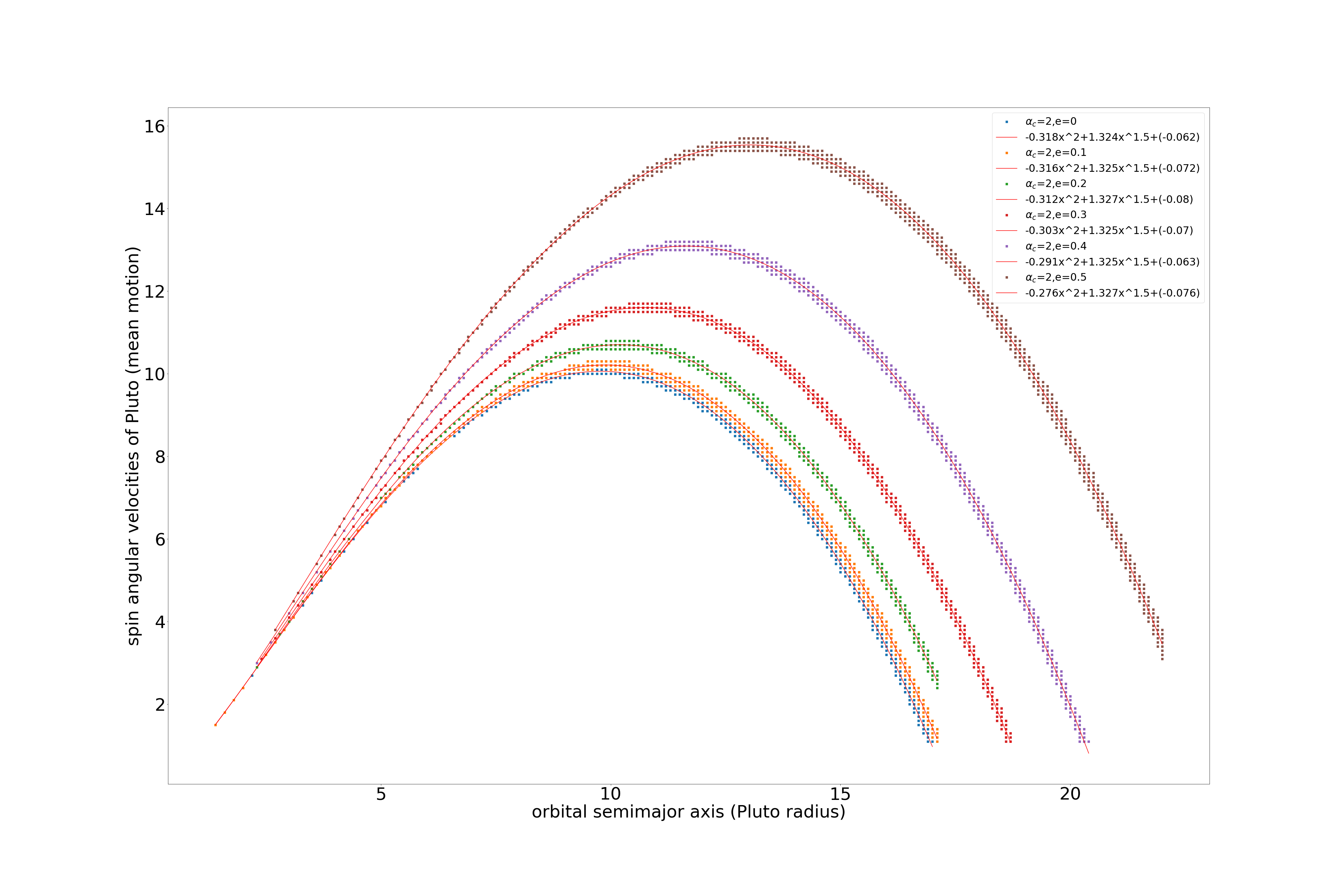
Figure 5: The possible initial state at $\alpha_{c}$=2, and e=0, 0.1, 0.2, 0.3, 0.4, 0.5

At figure 5, I set an initial $\alpha_{c}=2$ and change the initial eccentricity. And it is the same as figure 4. I test the orbital semi-major axis from 1 to 22 Pluto’s radius and Pluto’s spin velocity from 1 to 17 and if they can evolve to the current state (end X is $16.9<X<17.1$). Then, I plot this point in figure 5. Then, it also follows the equation (11).

The initial states satisfy angular momentum. If we want to find the initial state with the tidal evolution. We just use the conserving angular momentum. Besides, whenever they will follow the angular momentum. Show this fact, we can plot the $\alpha_{p}$ to X at evolution. Then, we can see evolution more clearly.

2.3 $\alpha_{p}-X$

Here, at our simulating, the endpoint of the initial state $\alpha_{p}$=5.3,$\alpha_{c}$=2, a=3.9, eccentricity e=0 is more approach to the current state X=17. Thus, we choose the initial state $\alpha_{p}$=5.5 and a=4 to demonstrate from figure 6 to figure 17.

Figure 6 to figure 9 is the different initial Charon’s spin velocity.

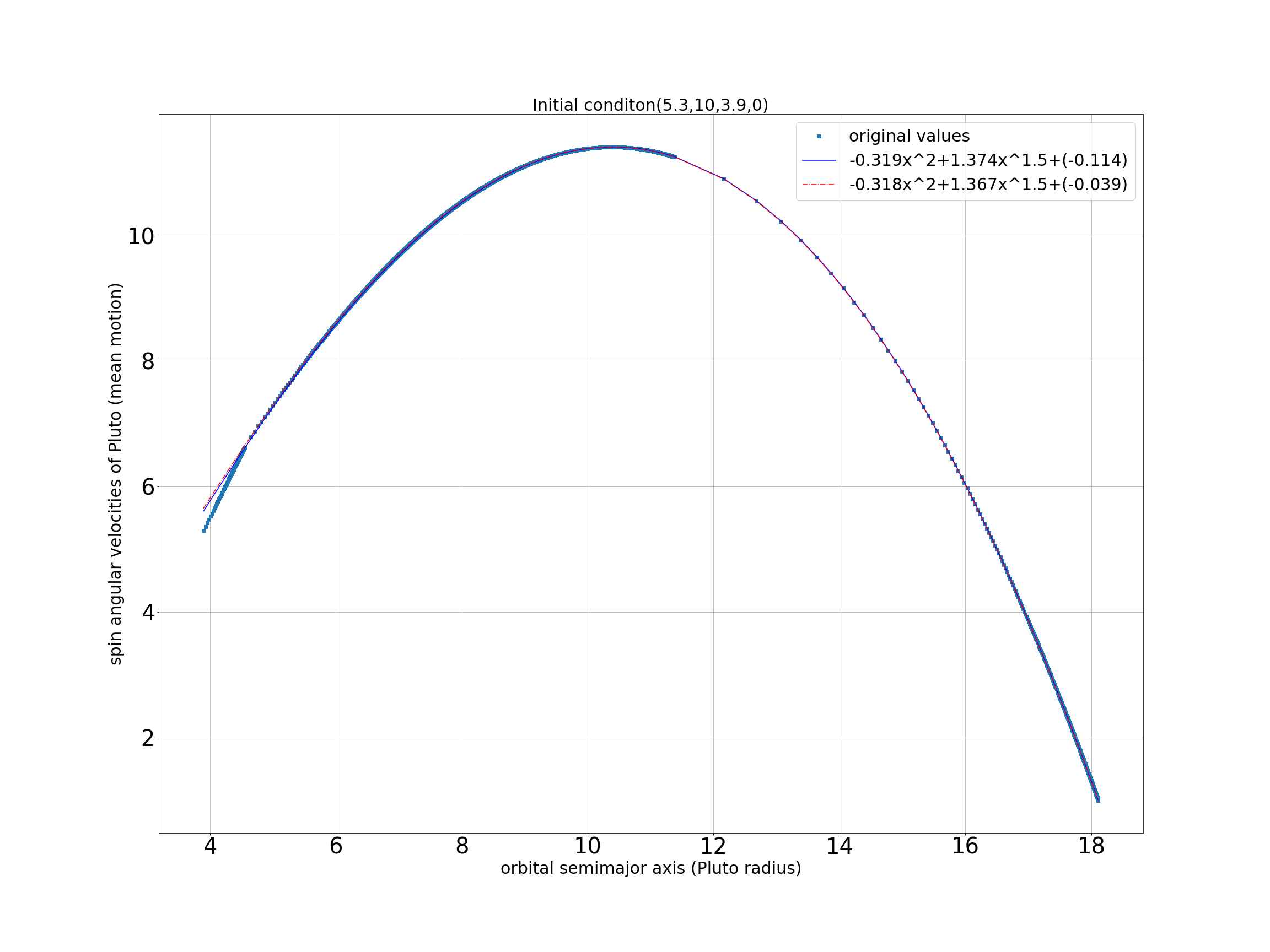
Figure 6: $\alpha_{p}$ vs X at tidal evolution, and its initial state is $\alpha_{p}$=5.3, $\alpha_{c}$=10, X=3.9, and e=0.

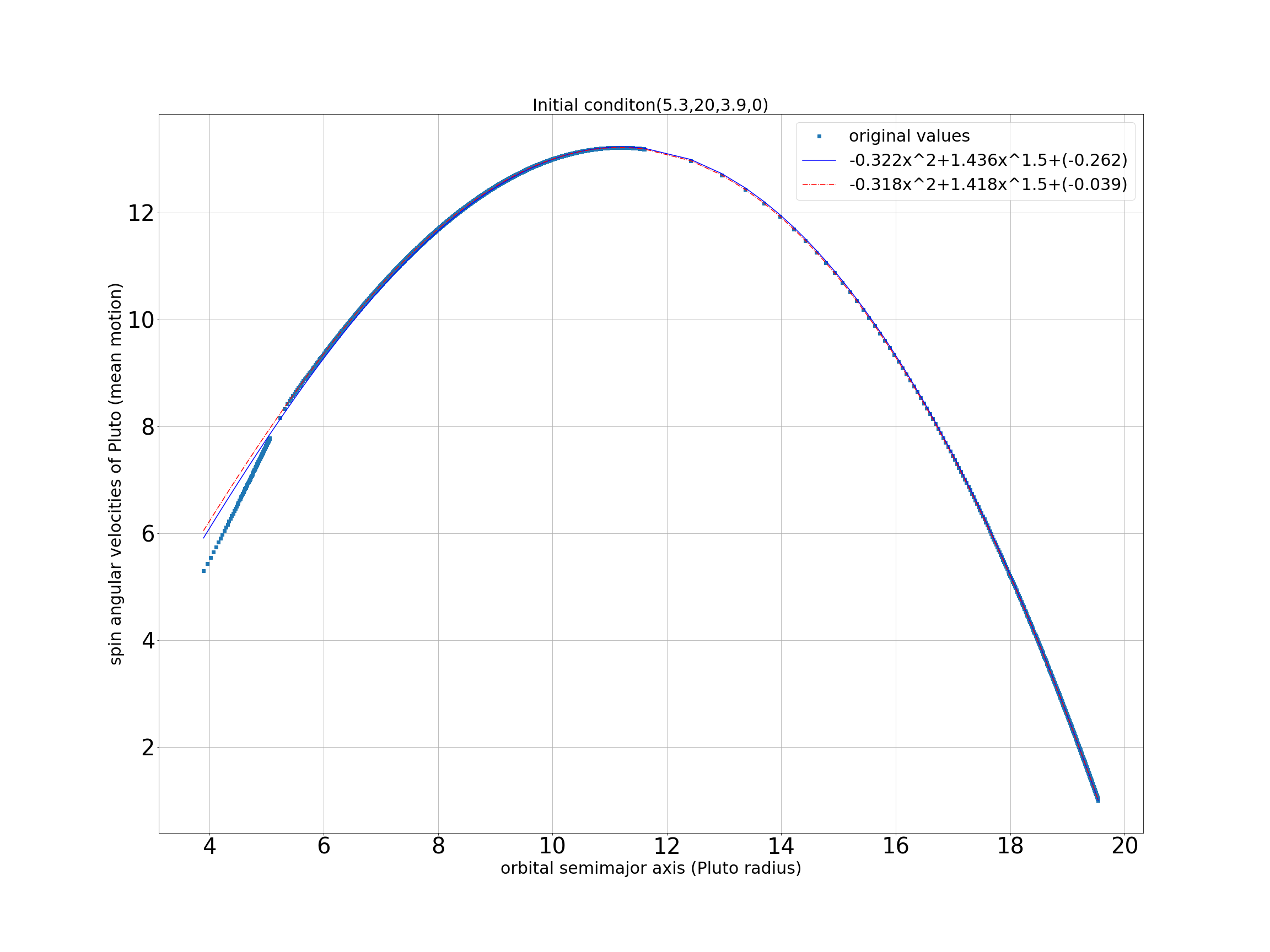
Figure 7: $\alpha_{p}$ vs X at tidal evolution, and its initial state is $\alpha_{p}$=5.3, $\alpha_{c}$=20, X=3.9, and e=0.

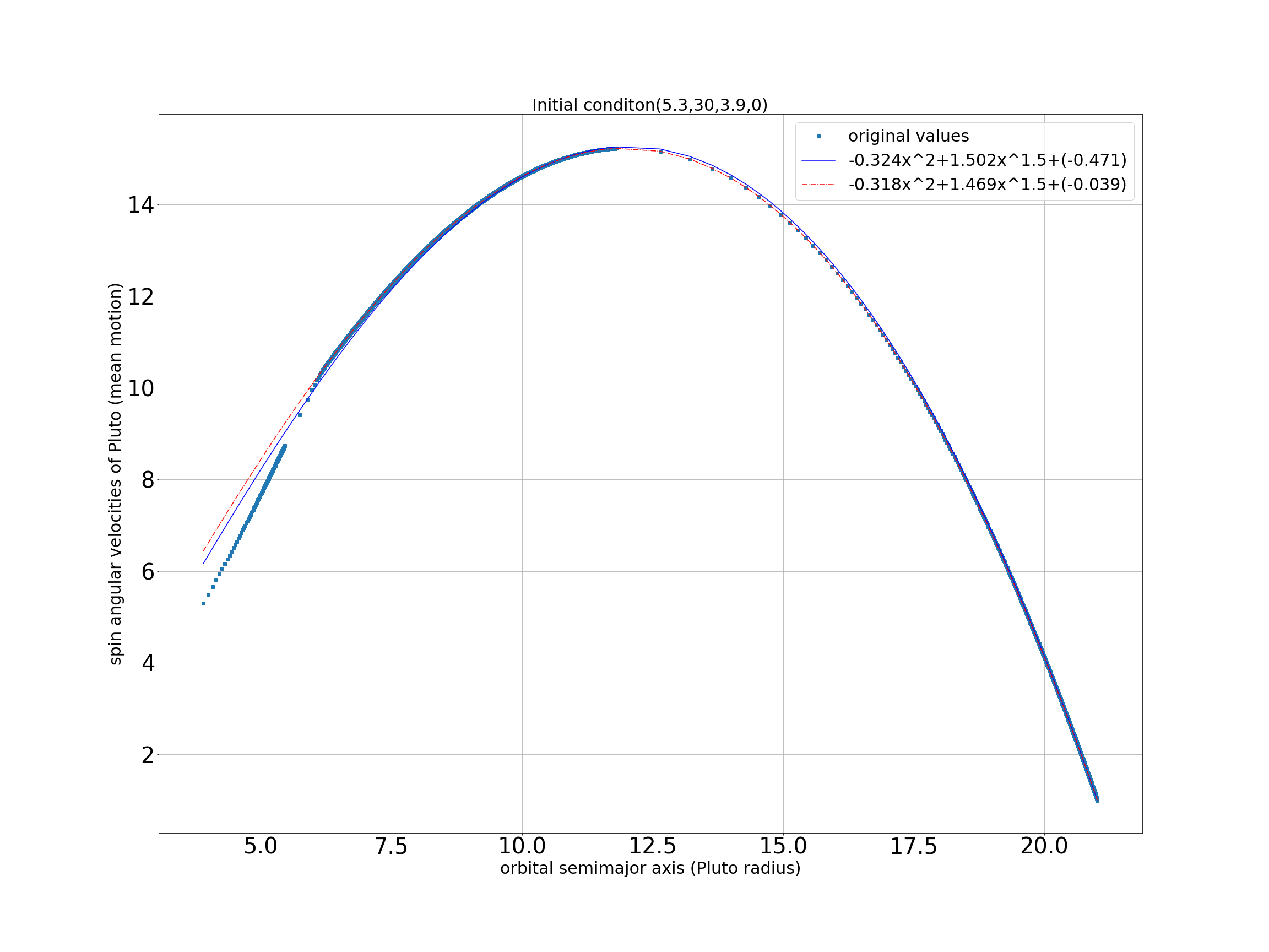
Figure 8: $\alpha_{p}$ vs X at tidal evolution, and its initial state is $\alpha_{p}$=5.3, $\alpha_{c}$=30, X=3.9, and e=0.

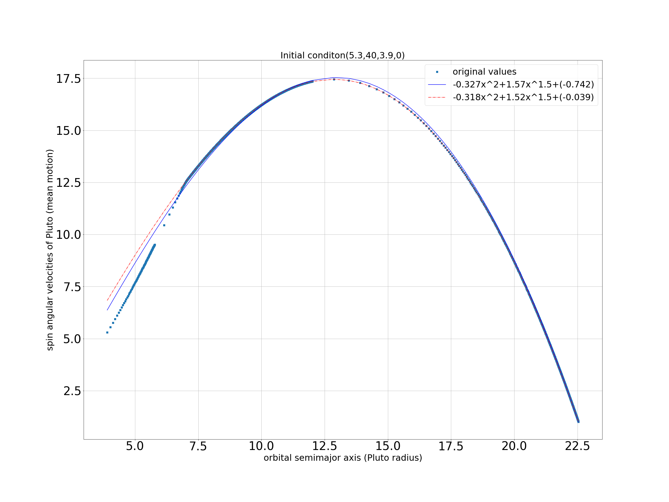
Figure 9: $\alpha_{p}$ vs X at tidal evolution, and its initial state is $\alpha_{p}$=5.3, $\alpha_{c}$=40, X=3.9, and e=0.

When we change the initial $\alpha_{c}$ it quickly decays to 1. Thus, if the eccentricity is 0, the Pluto-Charon spends a lot of time at the red dash curve which is the equation from conservation of angular momentum decided by the final state. It is the line follow e=0 and $\alpha_{c}=1$. (The blue point is from the tidal evolution equation, and the blue curve is the fitting line.)

The $\alpha_{c}$ will let the curve away obviously from the red dash curve at low $A_{\triangle t}$. Pluto-Charon’s tidal evolution is affected by the tidal force that Charon draws Pluto and Pluto draws Charon. Then, the $A_{\triangle t}$ decides how large the tidal force that Pluto draws Charon affects. Thus, at low $A_{\triangle t}$, the tidal force that Pluto draws Charon affects large. It will make the evolution away from the red curve. On the contrary, the high $A_{\triangle t}$ just let this evolution spend more time at the red dash curve. About the influence of $A_{\triangle t}$, we will talk the detail at the discussion.

The tidal evolution spends a lot of time at the red dot curve. This fact is very clearly can be thought from the Earth-Moon. Earth-Moon is at this stage. The spin velocity of the Moon almost be the same as the mean motion and the eccentricity is also 0.

Then, let us show the influence of different initial eccentricities from figure 10 to figure 17. This result is different from the result that we change the initial Charon’s spin velocity. At figure 6 $\sim$ 9, we can see a long period at the $\alpha_{c}=1$ and eccentricity equal 0. However, when we change the initial eccentricity. It is away from the red dash that the situation $\alpha_{c}=1$ and eccentricity equal 0. This part is a relation of $A_{\Delta t}$ and the overshoot. The influence of tidal force that Pluto draws Charon makes a very different evolution. The detail we will discuss at the discussion.

Besides, in figure $10\sim 17$, the trend of the initial state is not that the larger eccentricity is the more influential at the tidal evolution. At these figures, we find at the special section eccentricity is interesting for us. At this result, although we can’t find the initial state of Pluto-Charon with tidal evolution, if we want to the other star initial condition. If the current eccentricity isn’t 0. Of course, we want to check this star is almost sphere to make us ignore the permanent quadrupole moment. Then, we can shrink the range of their initial sate because it is difficult to make high eccentricity after tidal evolution.

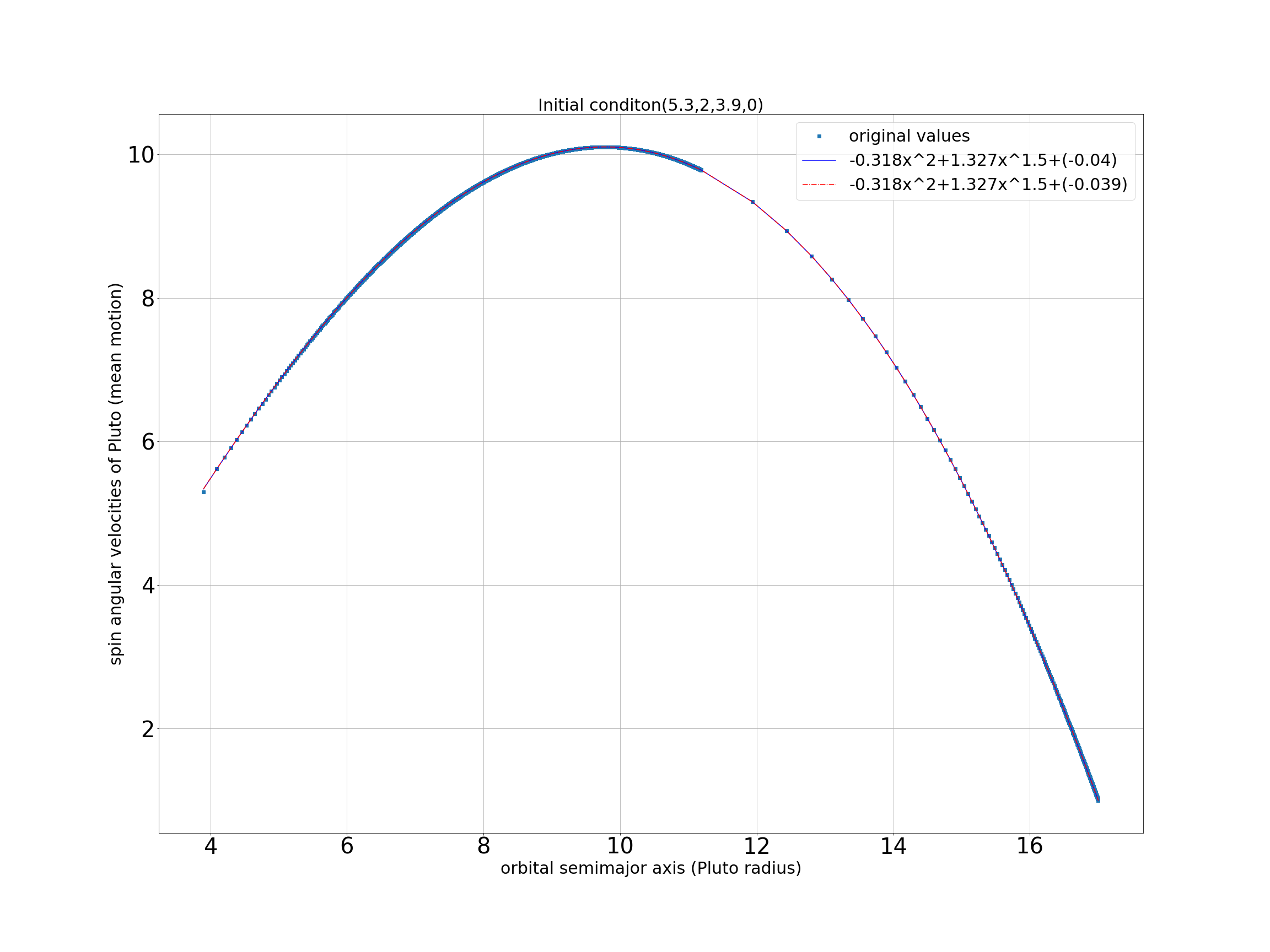
Figure 10: $\alpha_{p}$ vs X at tidal evolution, and its initial state is $\alpha_{p}$=5.3, $\alpha_{c}$=2, X=3.9, and e=0.

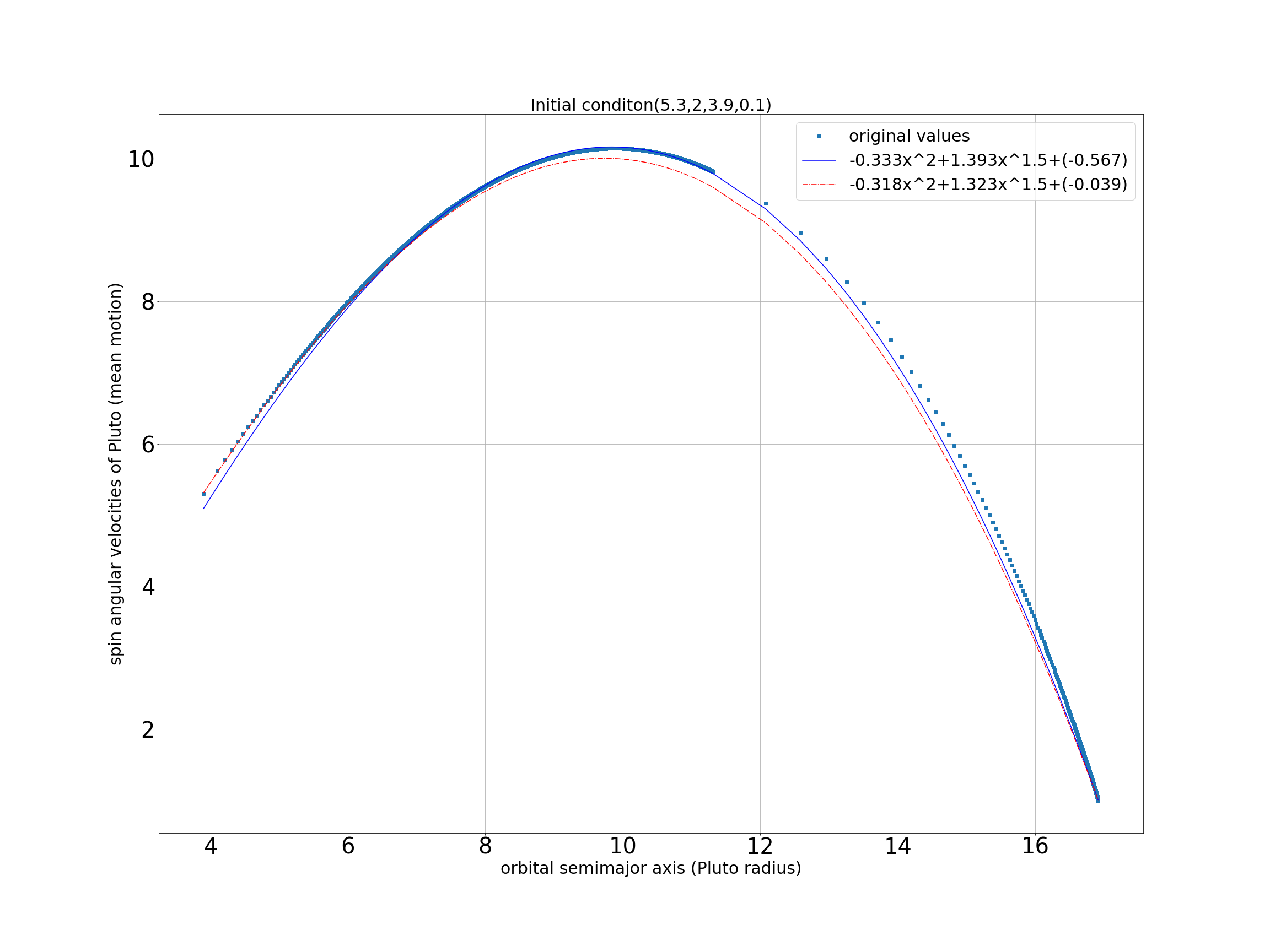
Figure 11: $\alpha_{p}$ vs X at tidal evolution, and its initial state is $\alpha_{p}$=5.3, $\alpha_{c}$=2, X=3.9, and e=0.1.

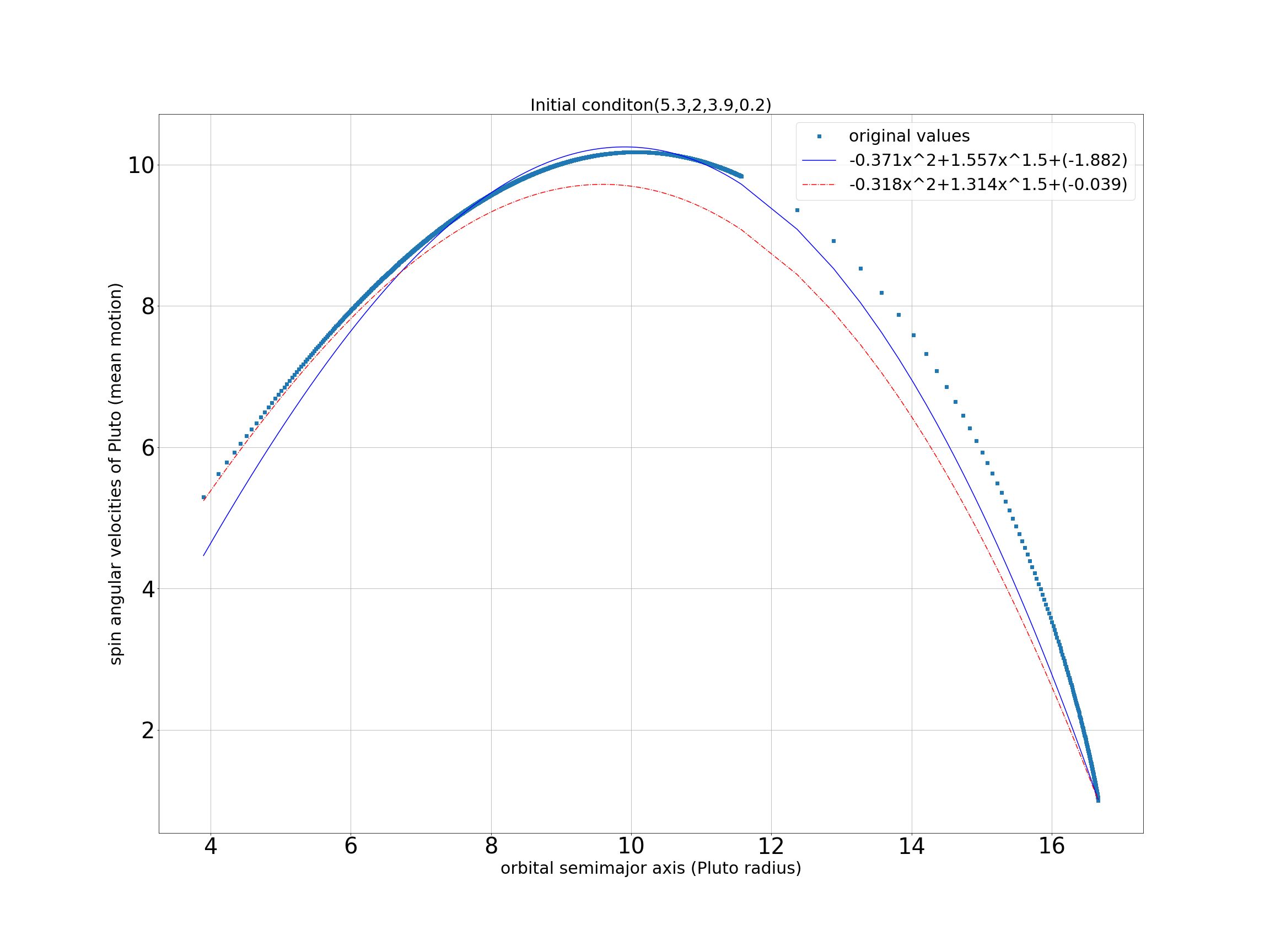
Figure 12: $\alpha_{p}$ vs X at tidal evolution, and its initial state is $\alpha_{p}$=5.3, $\alpha_{c}$=2, X=3.9, and e=0.2.

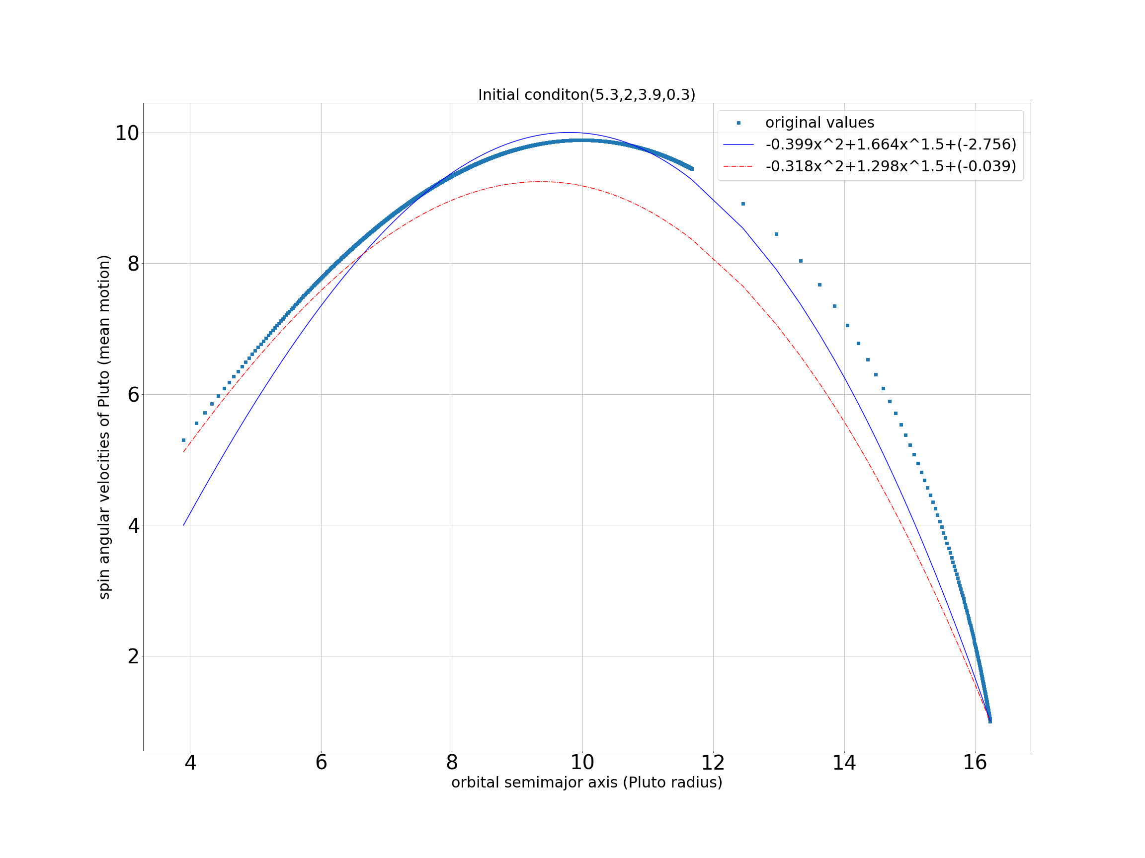
Figure 13: $\alpha_{p}$ vs X at tidal evolution, and its initial state is $\alpha_{p}$=5.3, $\alpha_{c}$=2, X=3.9, and e=0.3.

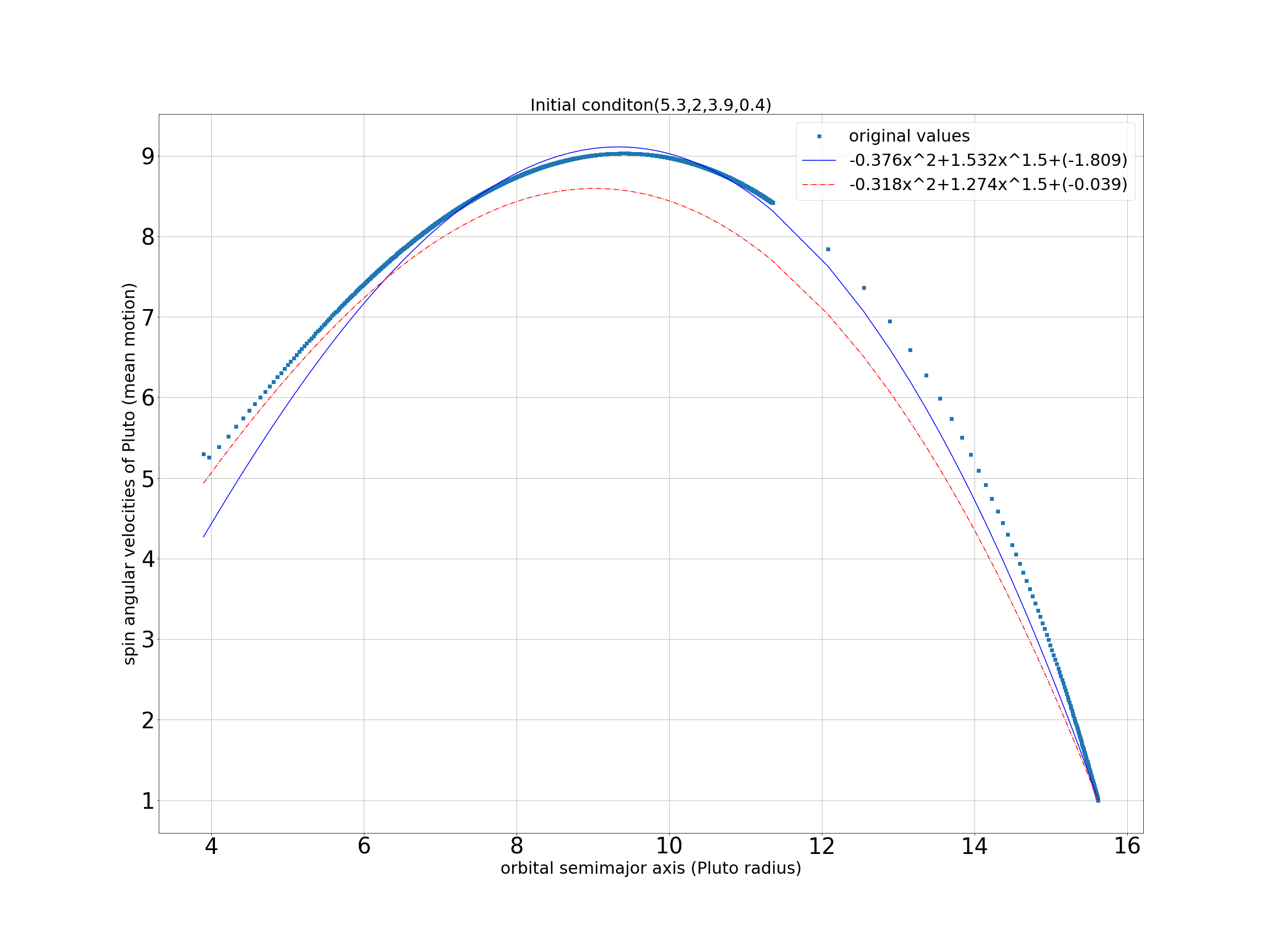
Figure 14: $\alpha_{p}$ vs X at tidal evolution, and its initial state is $\alpha_{p}$=5.3, $\alpha_{c}$=2, X=3.9, and e=0.4.

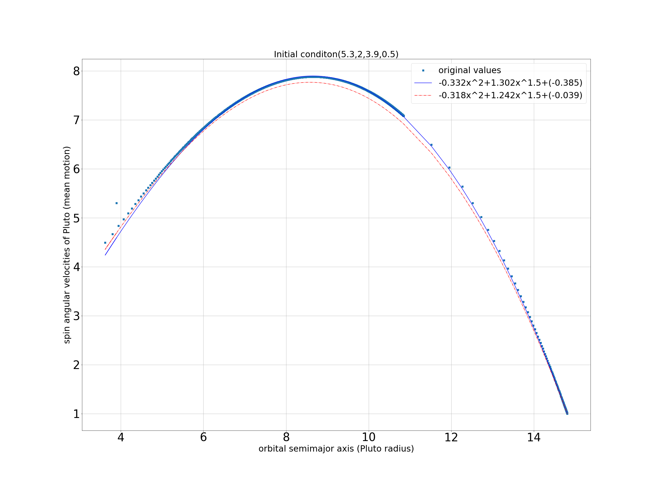
Figure 15: $\alpha_{p}$ vs X at tidal evolution, and its initial state is $\alpha_{p}$=5.3, $\alpha_{c}$=2, X=3.9, and e=0.5.

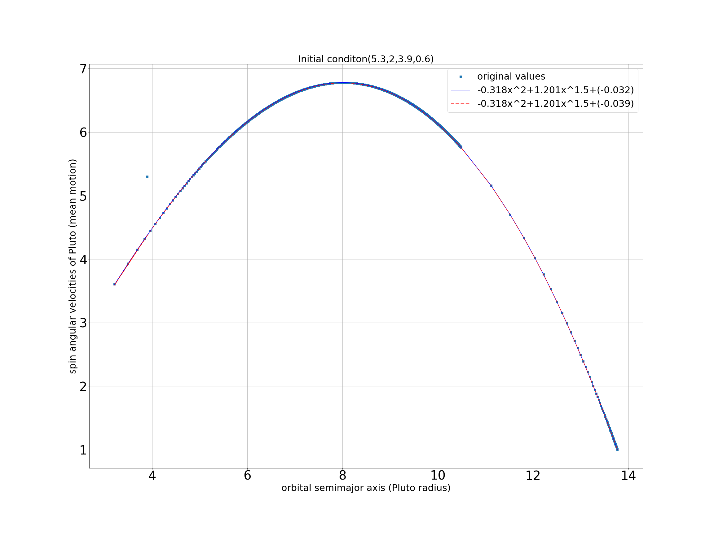
Figure 16: $\alpha_{p}$ vs X at tidal evolution, and its initial state is $\alpha_{p}$=5.3, $\alpha_{c}$=2, X=3.9, and e=0.6.

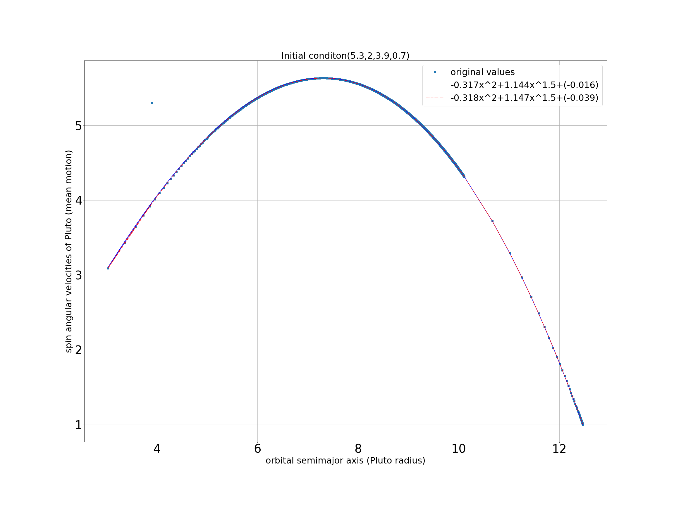
Figure 17: $\alpha_{p}$ vs X at tidal evolution, and its initial state is $\alpha_{p}$=5.3, $\alpha_{c}$=2, X=3.9, and e=0.7.

3.   Q model-solving the overshoot

From section 2, the truncation of the expansion makes orbital semi-major axis overshoot before coming back to the current state. We want to solve the unnecessary ”overshoot”. We can see the difference between figure 1 and figure 3. At $\Delta t$ model, figure 3 follows a complete equation of tidal evolution and figure 1 follows the truncation of the expansion of the tidal evolution equation. Thus, the unnecessary overshoot happens at the Q model because we use the truncation of the expanding tidal evolution from the Zahn 1977. Thus, I attempt to calculate the Q model like $\triangle t$ model. It contains all orders of eccentricity at $\triangle t$ model. Then, we follow the calculating way of P. Hut. By the definition from solar system dynamics. we let the $\sin 2\delta=-\frac{1}{Q}$. Then, the leading contribution to the tidal perturbing force.

$$F_{r}=-3G\frac{m^{2}}{r^{2}}(\frac{R}{r})^{5}k(1+3\frac{\dot{r}}{r}\frac{Q}{2\dot{\psi}-2\dot{\theta}})$$ (12)

$$F_{\theta}=-3G\frac{m^{2}}{r^{2}}(\frac{R}{r})^{5}k\frac{Q}{2})$$ (13)

Here, the perturbation of energy from $F_{\theta}$. It can be easy to get. However, the dissipation energy from $F_{r}$ the integrate to average the dissipation energy. In the integral term

$$\int_{0}^{2\pi}\frac{\sin^{2}\theta(1+cos\theta)^{6}}{\dot{\psi}-\frac{(1+cos\theta)^{2}}{(1-e^{2})^{3/2}}n}d\theta$$ (14)

When the $\frac{(1+cos\theta)^{2}}{(1-e^{2})^{3/2}}$ approach $\dot{\psi}$ we have the point limit to infinity. Then, when they approach. Their figure like that differential of Dirac delta function at $\pi/2$ minus differential of Dirac delta function at $3\pi/2$. Along with eccentricity changing, the diverging point of the Dirac delta function moves a bit. However, we still take the approach value at different $\dot{\psi}$ and n. It doesn’t satisfy our purpose to derive a containing all order eccentricity of the tidal evolution equation.

We know the reason for the overshoot is the problem that the equation doesn’t contain all orders of eccentricity. From section 2, we know the low eccentricity still contains the conservation of angular momentum. Thus, although we can’t calculate the expression contain all orders of eccentricity, we can show the more expansion at tidal evolution. Then, when the initial eccentricity equals to 0.3, the problem ”overshoot” won’t happen.

First, we’re from Zahn 1966 and then expand that to the order=4. The tidal potential is

$$U=\frac{GM_{c}}{a}\left(\frac{r}{a}\right)^{2}\cdot {\left[-\frac{1}{2}P_{2}(\cos\theta)\cdot\left(1+3e\cos\omega t+e^{2}\left(\frac{3}{2}+\frac{9}{2}\cos 2\omega t\right)\right.\right.}$$ (15)

$$\left.+e^{3}\left(\frac{27}{8}\cos\omega t+\frac{53}{8}\cos 3\omega t\right)+e^{4}\left(\frac{15}{8}+\frac{7}{2}\cos 2\omega t+\frac{77}{8}\cos 4\omega t\right)\right)$$

$$+\frac{1}{4}P_{2}^{2}(\cos\theta)\cdot\left(\left(\cos(\omega t-2\phi)+e\left(\frac{7}{2}\cos(3\omega t-2\phi)-\frac{1}{2}\cos(\omega t-2\phi)\right)\right.\right.$$

$$+e^{2}\left(\frac{17}{2}\cos(4\omega t-2\phi)-\frac{5}{2}\cos(2\omega t-2\phi)\right)$$

$$+e^{3}\left(\frac{1}{16}\cos(\omega t-2\phi)+\frac{1}{48}\cos(\omega t+2\phi)\right.$$

$$\left.+\frac{845}{48}\cos(5\omega t-2\phi)-\frac{123}{16}\cos(3\omega t-2\phi)\right)$$

$$+e^{4}\left(\frac{533}{16}\cos(6\omega t-2\phi)+\frac{1}{24}\cos(2\omega t+2\phi)\right.$$

$$\left.\left.\left.-\frac{115}{16}\cos(4\omega t-2\phi)+\frac{13}{16}\cos(2\omega t-2\phi)\right)\right)\right]+O\left(e^{5}\right)$$

Here, the r, $\theta$, and $\phi$ is the sphere coordinate, it is also mentioned at the Zahn’s paper (Zahn 1977). Then, we want to find perturbation acceleration. Like Zahn’s article, take the secondary center to be the origin point. The polar coordinates are (r, O, f-$\psi$ t). Then, from solar system dynamics, the definition of the mean anomaly is

$$f=\omega t+2e\sin\omega t+\frac{5}{4}e^{2}+e^{3}(\frac{13}{12}\sin 3\omega t-\frac{1}{4}\sin\omega t)$$

$$\phantom{f=M+2e\sin M+\frac{5}{4}e^{2}}+e^{4}(\frac{103}{96}\sin 4\omega t-\frac{11}{24}\sin 2\omega t)+O(e^{5})$$ (16)

Like Zahn 1977, to expand perturbing acceleration as Fourier series in $\omega$t and take the odd term as R and the even terms as S. Then, we express the perturbing acceleration at order 4. The radial component R and the tangential component S is:

$$R=-\frac{9}{4}\frac{Gm_{s}}{R^{2}}(\frac{R_{p}}{a})^{7}(\frac{a}{r})^{4}$$

$$\phantom{R}\cdot[e\sin\omega t(\epsilon_{2}^{10}+\frac{1}{4}\epsilon_{2}^{12}-4\epsilon_{2}^{22}+\frac{7}{2}\epsilon_{2}^{32})$$

$$\phantom{R}+e^{2}\sin 2\omega t(\frac{9}{4}\epsilon_{2}^{20}+\epsilon_{2}^{12}-\frac{5}{2}\epsilon_{2}^{22}-7\epsilon_{2}^{32}+\frac{17}{2}\epsilon_{2}^{42}]$$ (17)

$$S=-\frac{3}{2}\frac{Gm_{s}}{R^{2}}(\frac{R_{p}}{a})^{7}(\frac{a}{r})^{4}$$

$$\phantom{S}\cdot[\epsilon_{2}^{22}+e\cos\omega t(-\frac{1}{2}\epsilon_{2}^{12}+\frac{7}{2}\epsilon_{2}^{32})$$

$$\phantom{S}+e^{2}(\epsilon_{2}^{12}-\frac{13}{2}\epsilon_{2}^{22}+7\epsilon_{2}^{22})$$

$$\phantom{S}+e^{2}\cos 2\omega t(-\epsilon_{2}^{12}+4\epsilon_{2}^{22}-7\epsilon_{2}^{32}+\frac{17}{2}\epsilon_{2}^{42})$$

$$\phantom{S}+e^{3}\cos\omega t(\frac{27}{16}\epsilon_{2}^{12}-5\epsilon_{2}^{22}-\frac{165}{16}\epsilon_{2}^{32}+17\epsilon_{2}^{42})$$

$$\phantom{S}+e^{4}(-\epsilon_{2}^{12}+\frac{57}{4}\epsilon_{2}^{22}-39\epsilon_{2}^{32}+\frac{221}{8}\epsilon_{2}^{42})]$$ (18)

The term S has still some term at the order of 3 and order of 4, but when they are averaged, their term will be larger than order 4. i.e. The order of eccentricity is 6 by averaging $e^{3}\cos 3\omega t$.

Now, we follow the solar system dynamic chapter 2.9. The change of semi-major axis, eccentricity. And the spin velocity will follow torque $-M_{c}rS$ is:

$$\frac{d}{dt}a=\frac{2}{n\sqrt{1-e^{2}}}[e\sin{f}R+(1-e^{2})\frac{a}{r}S]$$ (19)

$$\frac{d}{dt}e=\frac{\sqrt{1-e^{2}}}{na}[\sin{f}R+(\cos{f}+\cos{E})S]$$ (20)

$$\frac{d}{dt}\dot{\psi}=-\frac{M_{2}}{C}rS$$ (21)

Now, we substitute the components R and S.

$$\frac{da}{dt}=-\frac{3}{n}\frac{M_{p}+M_{s}}{M_{p}}\frac{GM_{s}}{R_{p}^{2}}(\frac{R_{p}}{a})^{7}$$

$$\phantom{\frac{da}{dt}}\cdot[\epsilon_{2}^{22}+e^{2}(\frac{3}{4}\epsilon_{2}^{10}+\frac{1}{8}\epsilon_{2}^{12}-5\epsilon_{2}^{22}+\frac{147}{8}\epsilon_{2}^{32})$$

$$\phantom{\frac{da}{dt}}+e^{4}(\frac{32}{27}\epsilon_{2}^{10}+\frac{81}{16}\epsilon_{2}^{20}+\frac{115}{64}\epsilon_{2}^{12}-6\epsilon_{2}^{22}-\frac{3579}{64}\epsilon_{2}^{32}-\frac{527}{4}\epsilon_{2}^{42})+O(e^{6})]$$ (23)

$$\frac{de}{dt}=-\frac{3}{4}\frac{e}{n}\frac{M_{p}+M_{s}}{M_{p}}\frac{GM_{s}}{R_{p}^{3}}(\frac{R_{p}}{a})^{8}$$

$$\phantom{\frac{de}{dt}}\cdot[\frac{3}{2}\epsilon_{2}^{10}-\frac{1}{4}\epsilon_{2}^{12}-\epsilon_{2}^{22}+\frac{49}{4}\epsilon_{2}^{32}$$

$$\phantom{\frac{da}{dt}}+e^{4}(\frac{3}{16}\epsilon_{2}^{10}+\frac{81}{8}\epsilon_{2}^{20}+\frac{119}{32}\epsilon_{2}^{12}-\frac{45}{2}\epsilon_{2}^{22}-\frac{919}{32}\epsilon_{2}^{32}+119\epsilon_{2}^{42})+O(e^{6})]$$ (24)

$$\frac{d}{dt}(\dot{\psi}_{p})=\frac{3}{2}\frac{GM_{s}^{2}}{C_{p}R_{p}}(\frac{R_{p}}{a})^{6}$$

$$\phantom{\frac{d}{dt}(I\Omega)}\cdot[\epsilon_{2}^{22}+e^{2}(\frac{1}{4}\epsilon_{2}^{12}-5\epsilon_{2}^{22}+\frac{49}{4}\epsilon_{2}^{32})$$

$$\phantom{\frac{da}{dt}}+e^{4}(-\frac{1}{16}\epsilon_{2}^{12}+\frac{63}{8}\epsilon_{2}^{22}-\frac{861}{16}\epsilon_{2}^{32}+\frac{289}{4}\epsilon_{2}^{42})+O(e^{6})]$$ (25)

and we check this equation is true at $\triangle t$ model at order 4.We substitute $\epsilon_{2}^{lm}=k_{2}(ln-m\dot{\psi})\triangle t$

$$\frac{d\dot{\psi}_{i}}{dt}=-\frac{3G}{C_{i}}k_{2i}\triangle t_{i}{M_{j}}^{2}(\frac{R_{i}^{5}}{a^{6}})[(1+\frac{15}{2}e^{2}+\frac{105}{4}e^{4})\psi_{i}-(1+\frac{27}{2}e^{2}+\frac{573}{8}e^{4})n+O(e^{6})]$$ (26)

$$\frac{dX}{dt}=\frac{6G}{\mu X^{7}}k_{2p}\triangle t_{p}{M_{s}}^{2}(\frac{1}{R_{p}})^{3}[(1+\frac{27}{2}e^{2}+\frac{573}{8}e^{4})(\frac{\psi_{p}}{n}+A_{\triangle t}\frac{\psi_{c}}{n})$$

$$\phantom{\frac{dX}{dt}=\frac{6G}{\mu X^{7}}k_{2p}\triangle t_{p}{M_{s}}^{2}(\frac{1}{R_{p}})^{3}+{}}-(1+23e^{2}+180e^{4})(1+A_{\triangle t})+O(e^{4})]$$ (27)

$$\frac{de}{dt}=\frac{27eG}{\mu X^{8}}K_{2p}\triangle t_{p}{M_{s}}^{2}(\frac{1}{R_{p}})^{3}[\frac{11}{18}(1+\frac{13}{2}e^{2})(\frac{\dot{\psi_{p}}}{n}+A_{\triangle}t\frac{\dot{\psi_{s}}}{n})$$

$$\phantom{\frac{de}{dt}=\frac{27eG}{\mu X^{8}}K_{2p}\triangle t_{p}{M_{s}}^{2}(\frac{1}{R_{p}})^{3}}-(1+\frac{41}{4}e^{2})(1+A_{\triangle}t)+O(e^{2})]$$ (28)

After we check the tidal equation at $\triangle t$ model, let us expand it at Q model and simulate it.

$$\frac{d\dot{\psi_{i}}}{dt}=-\frac{3GM_{j}^{2}}{2C_{i}}\frac{k_{2i}}{Q_{i}}\frac{R_{i}^{5}}{a^{6}}[sgn(\dot{\psi}-n)+e^{2}D_{i}+e^{4}G_{i}+O(e^{6})]$$ (29)

$$\frac{1}{a}\frac{da}{dt}=3n\frac{k_{2p}}{Q_{p}}\frac{M_{c}}{M_{p}}(\frac{R_{p}}{a})^{5}[sgn(\dot{\psi}-n)+A_{Q}sgn(\dot{\psi}_{c}-n)$$

$$\phantom{\frac{1}{a}<\frac{da}{dt}>=3n\frac{k_{2p}}{Q_{p}}\frac{M_{c}}{M_{p}}(\frac{R_{p}}{a})^{5}}+e^{2}(E_{p}+A_{Q}E_{c})+e^{4}(H_{p}+A_{Q}H_{c})+O(e^{6})]$$ (30)

$$\frac{1}{e}\frac{de}{dt}=n\frac{k_{2p}}{Q_{p}}\frac{M_{c}}{M_{p}}(\frac{R_{p}}{a})^{5}[F_{p}+A_{Q}F_{c}+e^{2}(J_{p}+A_{Q}J_{c})+O(e^{4})]$$ (31)

Table 2: coefficient of (29)(30)(31)

$\dot{\psi}/n$	$D_{i}$	$E_{i}$	$F_{i}$	$G_{i}$	$H_{i}$	$J_{i}$
$>2$	15/2	51/4	57/8	105/4	2103/32	2937/64
$=2$	15/2	51/4	57/8	-46	-2113/32	-2775/64
$>3/2and<2$	15/2	51/4	57/8	-473/4	-6329/32	-8487/64
$=3/2$	-19/4	-45/8	-33/16	-1031/16	-9079/64	-14217/128
$>1and<3/2$	-17	-24	-45/4	-85/8	-1375/16	-2865/32
$=1$	-12	-19	-21/2	-37/2	-1279/16	-2325/32
$>1/2and<1$	-7	-14	-39/4	-211/8	-1183/16	-1785/32

Now, we show the figure. we simulate from (7)(8)(9). It is approaching in order 2. Here, this figure has unnecessary overshoot.

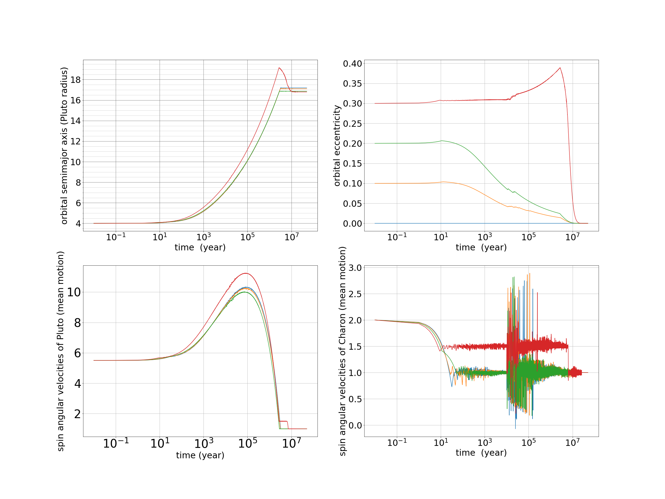
Figure 18: Tidal evolution at Q model follows (1)(2)(3) with $\epsilon_{2}^{lm}=\frac{k_{2}}{Q}sgn(ln-m\psi)$, and its initial state is $\alpha_{p}$=5.5, $\alpha_{c}$=2, X=4, and e=0.1, 0.2, and 0.3. The $A_{Q}$ is 1.15.

Then, we let the figure follow (29)(30)(31). I calculate the next term order of eccentricity. To simulate the eccentricity 0, 0.1, 0.2, 0.3. Then, the unnecessary overshoot is solved.

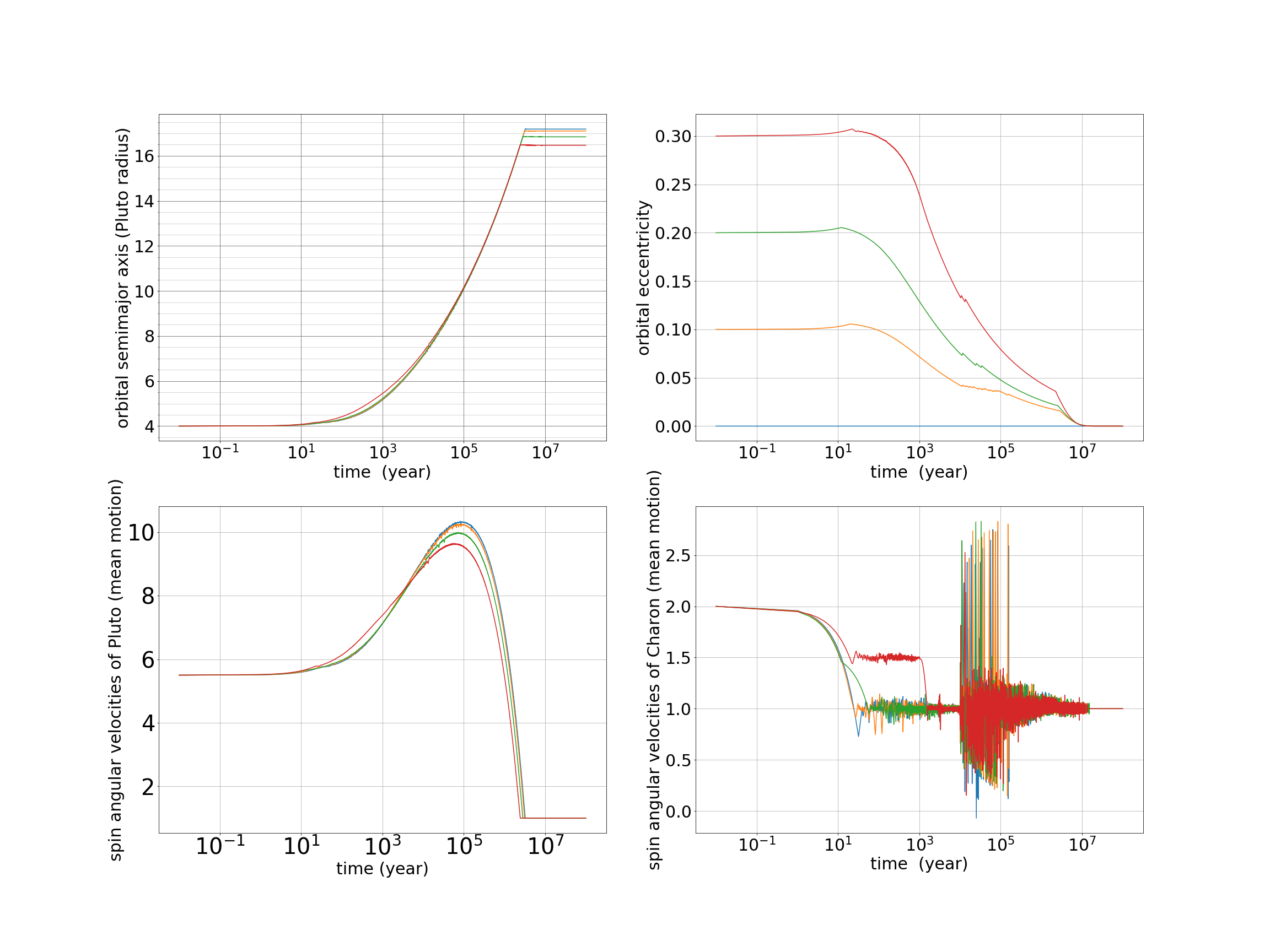
Figure 19: Tidal evolution at Q model follows (28)(29)(30), and its initial state is $\alpha_{p}$=5.5, $\alpha_{c}$=2, X=4, and e=0.1, 0.2, and 0.3.The $A_{Q}$ is 1.15.

However, this way isn’t a great way to solve the high eccentricity of the Q model. When we increase the eccentricity. This expression can’t still solve the high value of eccentricity. If we focus on the high eccentricity like that we say in section 2. If we want to use tidal evolution to shrink the range of initial state. We should be interested in the $0.2\sim 0.5$. The other initial $\alpha_{p}$ also changes the eccentricity. But we still consider a not low value at eccentricity when we want to use tidal evolution to research the other stars that its eccentricity isn’t zero. Then, the Q model isn’t good to simulate it. We would like to use a $\triangle t$ model to simulate it.

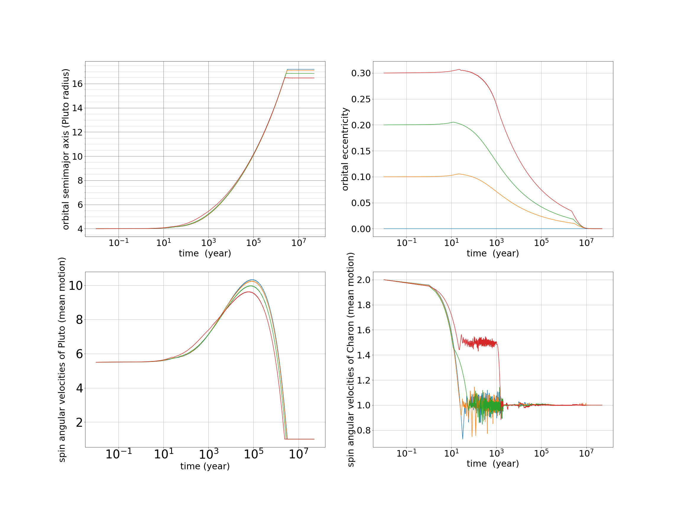
Figure 20: average 300 points of figure (19) after 2000yrs

In figure 20, we simulate the Q model is discontinue, I choose the absolute value smaller than $10^{-4}$, to imitate the sign function. At the later period, the $\alpha_{c}$ vibrating quickly. The following figure is that we average 300 points after 2000 years.

4.   tidal evolution including inclination

Even if the inclination of Charon is approaching zero, now. The initial inclination can’t still be ignored. The initial inclination is like the eccentricity. The end point of tidal evolution, the inclination is zero. Now, let us consider some value of inclination.

Here, let us be back to $\triangle t$ model. Although we have two ways to analyze the tidal evolution. However, the $\triangle t$ model is better since at our simulation. It isn’t an approach expression of tidal evolution. Now, we follow the equation from F. Mignard to consider inclination. The equation of tidal evolution including inclination:

$$\frac{1}{n}\frac{d\dot{\psi}_{i}}{dt}=-\frac{3G{M_{j}}^{2}}{C_{i}R_{i}}k_{2i}\triangle t_{i}(\frac{R_{i}}{a})^{6}[f_{1}(e)\frac{\psi_{i}}{n}cosI-f_{2}(e^{2})]$$ (32)

$$\frac{1}{a}\frac{da}{dt}=\frac{6G}{\mu R_{p}^{3}}k_{2p}\triangle t_{p}{M_{c}}^{2}(\frac{R_{p}}{a})^{8}[f_{2}(e^{2})(\frac{\psi_{p}}{n}cosI+A_{\triangle t}\frac{\psi_{c}}{n})$$

$$\phantom{\frac{dX}{dt}=\frac{6G}{\mu X^{7}}k_{2p}\triangle t_{p}{M_{s}}^{2}(\frac{1}{R_{p}})^{3}+{}}-f_{3}(e^{2})(1+A_{\triangle t})]$$ (33)

$$\frac{1}{e}\frac{de}{dt}=\frac{27G}{\mu R_{p}^{3}}K_{2p}\triangle t_{p}{M_{s}}^{2}(\frac{R_{p}}{a})^{8}[f_{4}(e^{2})\frac{11}{18}(\frac{\dot{\psi_{p}}}{n}cosI+A_{\triangle}t\frac{\dot{\psi_{s}}}{n})$$

$$\phantom{\frac{de}{dt}=\frac{27eG}{\mu X^{8}}K_{2p}\triangle t_{p}{M_{s}}^{2}(\frac{1}{R_{p}})^{3}}-f_{5}(e^{2})(1+A_{\triangle}t)]$$ (34)

$$\frac{dI}{dt}=\sum_{i}-\frac{3G}{C_{i}\ R_{i}}k_{2i}\triangle t_{i}{M_{s}}^{2}(\frac{R_{i}}{a})^{6}\frac{n}{\dot{\psi}_{p}}sinI[f_{2}(e^{2})$$

$$\phantom{\frac{dI}{dt}=-\frac{3G{M_{s}}^{2}}{C_{p}\ R_{p}}}-\frac{1}{2}(cosI-\frac{C_{i}}{\mu}(\frac{1}{a})^{2}(1-e^{2})^{-1/2}\frac{\dot{\psi}_{i}}{n})\frac{\dot{\psi}_{i}}{n}f_{1}(e^{2})]$$ (35)

$$f_{1}(e^{2})=(1+3e^{2}+\frac{3}{8}e^{4})/(1-e^{2})^{9/2}$$

$$f_{2}(e^{2})=(1+\frac{15}{2}e^{2}+\frac{45}{8}e^{4}+\frac{5}{16}e^{6})/(1-e^{2})^{6}$$

$$f_{3}(e^{2})=(1+\frac{31}{2}e^{2}+\frac{255}{8}e^{4}+\frac{185}{16}e^{6}+\frac{25}{64}e^{8})/(1-e^{2})^{15/2}$$

$$f_{4}(e^{2})=(1+\frac{3}{2}e^{2}+\frac{1}{8}e^{4})/(1-e^{2})^{5}$$

$$f_{5}(e^{2})=(1+\frac{15}{4}e^{2}+\frac{15}{8}e^{4}+\frac{5}{64}e^{6})/(1-e^{2})^{13/2}$$

The figure 21 shows the inclination decays quickly. And the tidal evolution isn’t influenced by inclination. Even if we change the inclination to $90^{\circ}$. And the figure (22) checks the different eccentricities don’t still change the fact the inclination doesn’t influence the tidal evolution.

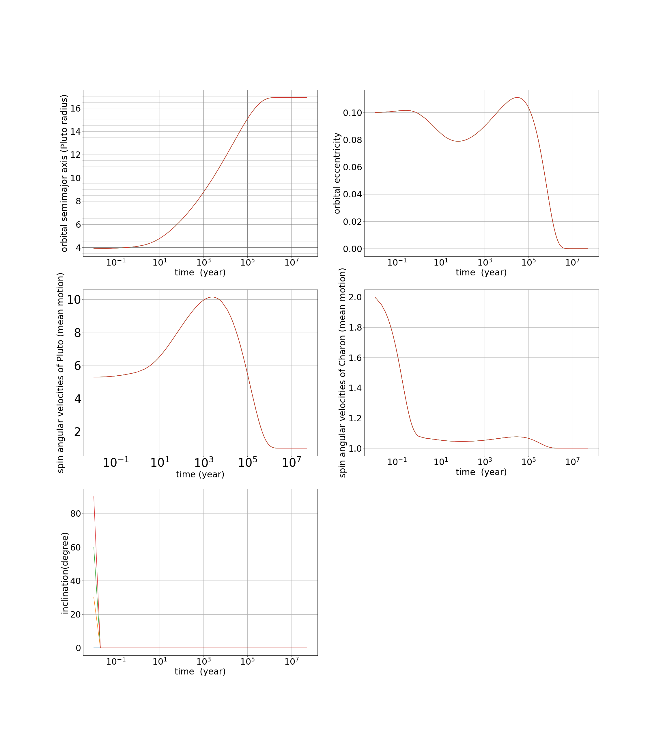
Figure 21: The different initial inclination doesn’t affect the evolution The initial state is that $\alpha_{p}$=5.5, $\alpha_{p}$=2 X=4, and e=0.1, and choose different inclination = $0^{\circ}$, $30^{\circ}$, $60^{\circ}$, and $90^{\circ}$

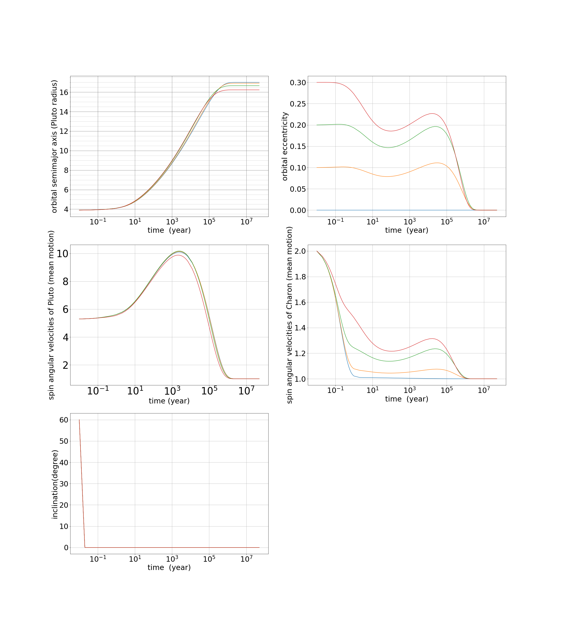
Figure 22: When we change the initial eccentricity, it doesn’t still affect evolution. The initial state is that inclination equals $60^{\circ}$, $\alpha_{p}$=5.5, $\alpha_{p}$=2 X=4, and choose different eccentricity = 0, 0.1, 0.2, and 0.3.

5.   Discussion

5.1 The influence of $A_{\triangle t}$ and $A_{Q}$

The $Q_{p}$ and $\triangle t_{p}$ influence all the speed of evolution. It moves the peak of $\alpha_{p}$, it doesn’t just influence the trend of tidal evolution. On the other hand, the $A_{\triangle t}$ and $A_{Q}$ will perturb this evolution. When the larger $A_{\triangle t}$ and $A_{Q}$, the eccentricity, and $\alpha_{c}$ decays quickly. This result is boring. On the contrary, the lower $A_{\triangle t}$ and $A_{Q}$ will make the eccentricity and $\alpha_{c}$ decays slowly. The perturbation is remarkable. Also, the result is the same as Cheng say, the too small $A_{\triangle t}$ and $A_{Q}$ will let the eccentricity can’t converge to 0. And this perturbation also makes an influence at the overshoot. When the eccentricity becomes larger, the orbital semi-major axis must be larger. We can’t avoid the overshoot. The overshoot is the normal phenomenon.

Then, we can find an interesting result. The tidal force will make stars spin fast and contain the high orbital semi-major axis. And this time, it has high eccentricity. The figure 22 shows this fact.

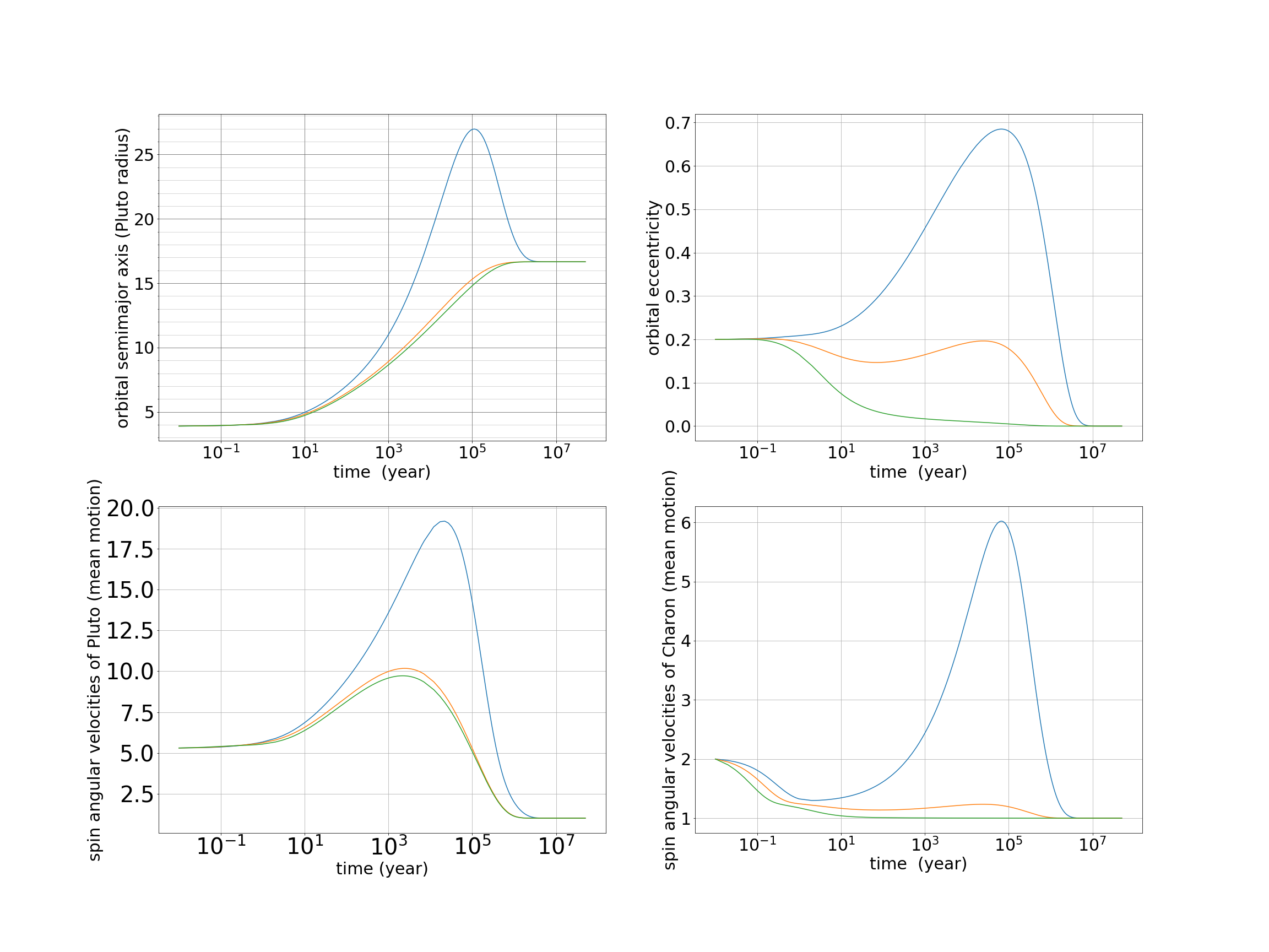
Figure 23: This figure shows that the influence of $A_{\Delta t}$ is important. The red line is $A_{\Delta t}=20$. The green line is $A_{\Delta t}=10$. The blue line is $A_{\Delta t}=5$. This initial state is that $\alpha_{p}=5.3$, $\alpha_{p}=2$ $X=3.9$,and $e=0.2$.

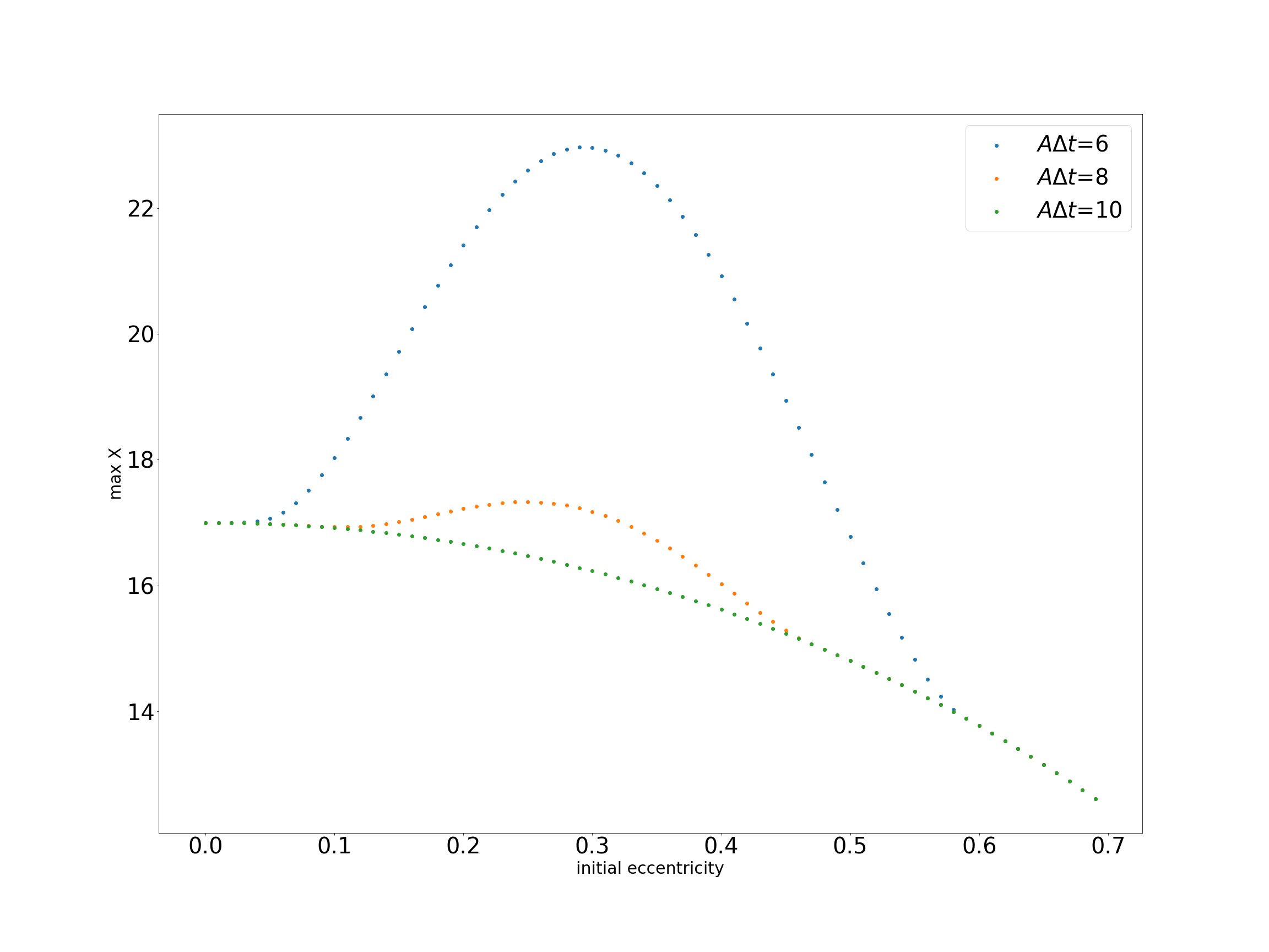
Figure 24: This figure Show the max $X$ at different initial eccentricity with $\triangle$ model. Initial state is that $\alpha_{p}$=5.3, $\alpha_{p}$=2 X=3.9, and choose different eccentricity at X axis.

As the last of section 2, the larger eccentricity doesn’t necessarily give the more influence at evolution. In figure 24, we show the relation between max X and initial at different $A_{\triangle t}$. In the high $A_{\triangle t}$, this phenomenon will not exist. But this phenomenon is still interesting. It’s difficult to investigate the Q or $\triangle t$. And this phenomenon doesn’t happen easily at the planet and satellite. In general planet and satellite, we ignore the influence of satellite. Thus, it is a good begin to start to research the binary stars. And, the high $A_{\triangle t}$ will result in this phenomenon.

6.   Conclusion

In section 2, we verify the Cheng’s result. To find the different eccentricity still satisfies the conservation of angular momentum. Then, we show some initial state at special eccentricity and spin velocity of Charon. It is very identical to the conservation of angular momentum. Then, we would like to know the evolution of the orbital semi-major axis. Because $\alpha_{p}$ to X. It should have a perfect fitting curve at a later period. Here, it is influenced by $A_{\triangle t}$ and $A_{Q}$. Here, we don’t seem to find a good evolution for Pluto-Charon. Because we can’t find the $A_{\triangle t}$ and $A_{Q}$. And, the $A_{\triangle t}$ and $A_{Q}$ influence the trend of tidal evolution, severely. The model tidal evolution is more powerful to find the binary stars still suffer the tidal evolution impacts.

In, section 3, we can find some problems from section 2 about the truncation of the order of eccentricity. We try a more accurate equation of the Q model to decrease the tendency of overshoot. However, when the $A_{Q}$ decrease the eccentricity will converge to 1. Although it happens possibly, the truncation of eccentricity will be inaccuracy at the low $A_{Q}$. Thus, we prefer to use a $\triangle t$ model to describe the tidal evolution.

In the next section, we just use $\triangle t$ to add the influence of inclination. Compare to the other parameter, the inclination decays quickly. It seems not important to consider the inclination of tidal evolution.

At last, we reconsider some special conditions from the overshoot. We choose the different eccentricity to find the max value X and $\alpha_{p}$ at the low $A_{\triangle t}$. It shows that it has a high semi-major axis, high spin velocity, and high eccentricity. At this condition, the character of the star has a very different state. The temperature at a star is also very different since the high variation of the orbital semi-major axis. We should attach importance to tidal evolution at binary stars with low A. In the future, we can focus to find some binary stars. They have the low A. At the condition, we can analyze the binary star. The tidal force will be important for us before we consider the other parameters.

References

- [1] Canup, R.M., 2005. A giant impact origin of Pluto-Charon. Science 307, 546–550
- [2] Canup, R.M., 2011. On a giant impact origin of Charon, Nix, and Hydra. The Astronomical Journal, 141, 35
- [3] Cheng, W.H., Lee, M.H., Peale, S.J., 2014. Complete tidal evolution of Pluto-Charon. Icarus 233, 242–258
- [4] Hut, P., 1981. Tidal evolution in close binary systems. Astron. Astrophys. 99, 126–140
- [5] Kopal, Zdenek, 1978. Dynamics of Close Binary Systems D. Reidel Publishing Company, Dordrecht, Holland
- [6] Mignard, F., 1980. The evolution of the lunar orbit revisited. II. Moon Planets 23, 185–201
- [7] Mignard, F., 1981. The lunar orbit revisited. III. Moon Planets 24, 189–207
- [8] Murray, C.D., Dermott, S.F., 1999. Solar System Dynamics. Cambridge Univ. Press, Cambridge
- [9] Zahn, J.P., 1966. Les marées dans une étoile double serrée. Ann. Astrophys. 29, 489
- [10] Zahn, J.P., 1977. Tidal friction in close binary stars. Astron. Astrophys. 57, 383–394