Task Adaptive Parameter Sharing for Multi-Task Learning

Abstract

Adapting pre-trained models with broad capabilities has become standard practice for learning a wide range of downstream tasks. The typical approach of fine-tuning different models for each task is performant, but incurs a substantial memory cost. To efficiently learn multiple downstream tasks we introduce Task Adaptive Parameter Sharing (TAPS), a general method for tuning a base model to a new task by adaptively modifying a small, task-specific subset of layers. This enables multi-task learning while minimizing resources used and competition between tasks. TAPS solves a joint optimization problem which determines which layers to share with the base model and the value of the task-specific weights. Further, a sparsity penalty on the number of active layers encourages weight sharing with the base model. Compared to other methods, TAPS retains high accuracy on downstream tasks while introducing few task-specific parameters. Moreover, TAPS is agnostic to the model architecture and requires only minor changes to the training scheme. We evaluate our method on a suite of fine-tuning tasks and architectures (ResNet, DenseNet, ViT) and show that it achieves state-of-the-art performance while being simple to implement.

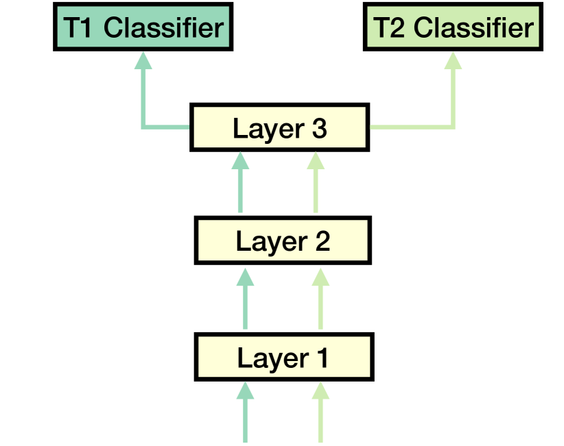
(a) Feature Extractor

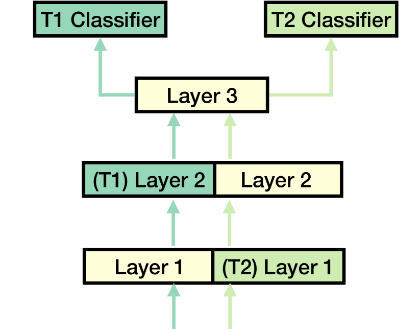
(b) Our Method

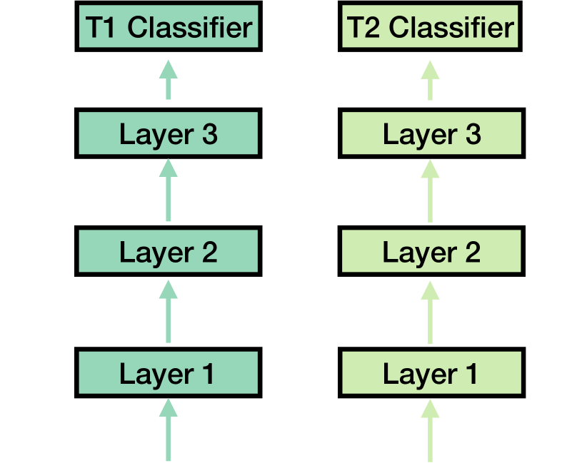
(c) Fine-Tuning

Figure 1: Overview of our approach. Difference between (b) our approach, (a) feature extractor as well as (c) finetuning. Here we have two tasks $T_{1}$ and $T_{2}$. $T_{1}$ shown by turquoise and $T_{2}$ by green. Yellow boxes denote the base network layer. Our approach adds task specific parameters to different layers based on the target tasks. Notice that this is in contrast to (a) no task specific layers are used and (c) where every layer is tasks specific. Also (c) suffers from catastrophic forgetting, and lose the base network’s parameters unlike (b) and (a).

1 Introduction

Real-world applications of deep learning frequently require performing multiple tasks (Multi-Task Learning/MTL). To avoid competition between tasks, a simple solution is to train separate models starting from a common pre-trained model. Although this approach results in capable task-specific models, the training, inference, and memory cost associated grows quickly with the number of tasks. Further, tasks are learned independently, missing the opportunity to share when tasks are related.

Ideally, one would train a single model to solve all tasks simultaneously. A common approach is to fix a base model and add task-specific parameters (e.g., adding branches, classifiers) which are trained separately for each task. However, deciding where to branch or add parameters is non-trivial since the optimal choice depends on both the initial model and the downstream task, to the point that some methods train a secondary network to make these decisions.

Moreover, adding weights (layers, parameters, etc.) to a network independent of the task is also not ideal: some methods  [23, 34, 18] add a small, fixed number of learnable task-specific parameters, however they sacrifice performance when the downstream task is dissimilar from the pre-training task. Other methods perform well on more complex tasks, but add an excessive number of task-specific parameters even when the downstream task is simple [40, 9, 50]

In this work, we overcome these issues by introducing Task Adaptive Parameter Sharing (TAPS). Rather than modifying the architecture of the network or adding a fixed set of parameters, TAPS adaptively selects a minimal subset of the existing layers and retrains them. At first sight, selecting the best subset of layers to adapt is a complex combinatorial problem which requires an extensive search among $2^{L}$ different configurations, where $L$ is the number of layers. The key idea of TAPS is to relax the layer selection to a continuous problem, so that deciding which layers of the base model to specialize into task-specific layers can be done during training by solving a joint optimization using stochastic gradient descent.

The final result is a smaller subset of task-specific parameters (the selected layers) which replace the base layers. Our approach has several advantages: (i) It can be applied to any architecture and does not need to modify it by introducing task-specific branches; (ii) TAPS does not reduce the accuracy of the target task (compared to the paragon of full fine-tuning) while introducing fewer task-specific parameters; (iii) The decision of which layers to specialize is interpretable, done with a simple optimization procedure, and does not require learning a policy network; (iv) It can be implemented in a few lines, and requires minimal change to the training scheme.

Our method finds both intuitive sharing strategies, and other less intuitive but effective ones. For example, TAPS tends to modify the last few layers for ResNet models while for Vision Transformers TAPS discovers a significantly different sharing pattern, learning to adapt only the self-attention layers while sharing the feed-forward layers.

We test our method on standard benchmarks and show that it outperforms several alternative methods. Moreover, we show that the results of our method are in-line with the standard fine-tuning practices used in the community. The contributions of the paper can be summarized as follows:

1. We propose TAPS, a method for differentiably learning which layers to tune when adapting a pre-trained network to a downstream task. This could range from adapting or specializing an entire model, to only changing $0.1\%$ of the pre-trained model, depending on the complexity/similarity of the new task.

2. We show that TAPS can optimize for accuracy or efficiency and performs on par with other methods. Moreover, it automatically discovers effective architecture-specific sharing patterns as opposed to hand-crafted weight or layer sharing schemes.

3. TAPS enables efficient incremental and joint multi-task learning without competition or forgetting.

2 Related Work

Multi-Domain and Incremental Multi-Task Learning

In many applications, it is desirable to adapt one network to multiple visual classification tasks or domains (Multi-Domain Learning, or MDL). Unlike Multi-Task Learning (MTL) where the tasks are learned simultaneously, in MDL the focus is to learn the domains incrementally, as often not all data is available at once. Accordingly, in this work, we also refer to MDL as incremental MTL. The standard approach for adapting a network to a single downstream task is fine-tuning. However, adapting to multiple domains incrementally poses the challenge of catastrophically forgetting previously learned tasks. To foster research in the area, Rebuffi et al. [34] introduced the Visual Decathlon challenge and proposed residual adapters. Residual adapters fix most of the network while training small residual modules that adapt to new domains. This architecture was modified to a parallel adapter architecture in [35]. A controller based method called Deep Adaptation (DA) was introduced in [37] to modify the learning algorithm using existing parameters. A simpler approach of using binary masks was proposed in Piggyback [23]. Task specific masks are learned then applied to the weights of the original network. This approach was further extended in Weight Transformations using Binary Masks (WTPB) [25] by modifying how the masks are applied. These methods focus on adding a small number of new parameters per task and underperform on more complex tasks as they have fixed capacity. Other solutions such as SpotTune [9] focus on performance without consideration for parameter efficiency. It trains an auxiliary policy network that decides whether to route each sample through a shared layer or task-specific layer. In contrast, TAPS does not require modification of the network architecture via adapters or training an auxiliary policy network. TAPS trains in one run with the same base architecture and requires no additional inference compute.

Parameter Efficient Multi-Domain Learning (MDL)

Another line of work in MDL is that of parameter sharing [27, 24]. These approaches typically perform multi-stage training. NetTailor [27] leverages the intuition that simple tasks require smaller networks than more complex tasks. They train teacher and student networks using knowledge distillation and a three-stage training scheme. PackNet [24] adds multiple tasks to a single network by iterative pruning. However, pruning weights generally causes performance degradation. More recently, Berriel et al. proposed Budget-Aware Adapters (BA²) [2]. This method selects and uses feature channels that are relevant for a task. Using a budget constraint, a network with the desired complexity can be obtained. In summary, most efficient parameter methods obtain efficiency at the loss of performance. Even with the largest budget in $BA^{2}$, the performance is substantially lower compared to TAPS. Unlike existing methods, TAPS does not need to choose a high accuracy or a high efficiency regime. As shown in Fig. 2, for a given task we can obtain models anywhere along the accuracy-efficiency frontier.

Multi-Task Learning (MTL)

MTL focuses on learning a diverse set of tasks in the same visual domain simultaneously by sharing information and computation, usually in the form of layers shared across all tasks and specialized branches for specific tasks [14, 32]. A few methods have attempted to learn multi-branch network architectures [20, 47] and some methods have sought to find sharing parameters among task-specific models [26, 38, 8]. A closely related work is AdaShare [46], which learns a task-specific policy that selectively chooses which layers to execute for a given task in the multitask network. They use Gumbel Softmax Sampling [21, 12] to learn the layer sharing policy jointly with the network parameters through standard back-propagation. Since this approach skips layers based on the task, it can only be applied to a subset of existing architectures where the input and output dimension of each layer is constant. Additionally because the sharing policy is trained jointly across all tasks, AdaShare cannot learn in the incremental setting.

Incremental Learning

Related to MDL is the problem of incremental learning. Here, the goal is to start with a few classes and incrementally learn more classes as more data becomes available. There are two approaches in this regard, methods that add extra capacity [40], [50] (layer, filter, etc.) and methods that do not[3, 13, 36, 19]. Methods that do not add extra capacity mitigate catastrophic forgetting by either using a replay buffer [3, 36] or minimizing changes to the weights [13]. Similar to our method, [40, 50] add capacity to the network to accommodate new tasks and prevent catastrophic forgetting. Progressive network [40] adds an entire network of parameters while Side-Tune [50] adds a smaller fixed-size network. Adding fixed capacity independent of the downstream task is sub-optimal since less complex tasks require fewer added parameters. In the extreme case where the pretrain task matches the downstream task no additional parameters are needed. In contrast to previous methods, TAPS adaptively adds capacity based on the downstream task and base network. Further, the goal of TAPS differs from incremental learning in that it starts with a pre-trained base model and learns new tasks or domains as opposed to adding new classes from a similar domain.

3 Approach

Given a pre-trained deep neural network with $L$ layers of weights and a set of $K$ target tasks $\mathcal{T}=\{T_{1},T_{2},...,T_{K}\}$, for each task we want to select the minimal necessary subset of layers that needs to be tuned to achieve the best (or close to the best) performance. This allows us to learn new tasks incrementally while adding the fewest new parameters. In principle, this requires a combinatorial search over $2^{L}$ possible subsets. The idea of Task Adaptive Parameter Sharing (TAPS) is to relax the combinatorial problem into a continuous one, which will ultimately give us a simple joint loss function to find both the optimal task-specific layers to tune and optimize parameters of those layers. An overview of our approach is shown in Fig. 1.

Weight parametrization

We first introduce a scoring parameter $s_{i}$ for each shared layer, where $i=1,\ldots,L$. We then reparametrize the weights of each layer as:

$$w_{i}=\bar{w}_{i}+I_{\tau}(s_{i})\,\delta w_{i},$$ (1)

where $\bar{w}_{i}$ are the (shared) weights of the pre-trained network and $\delta w_{i}$ is a trainable parameter which describes a task-specific perturbation of the base network. The crucial component is the indicator function $I_{\tau}(s_{i})$ defined by

$$I_{\tau}(s_{i})=\left\{\begin{array}[]{ c l }1&\quad\textrm{if }s_{i}\geq\tau,\\ 0&\quad\textrm{otherwise.}\end{array}\right.$$ (2)

for some threshold $\tau$. Hence, when $s_{i}\geq\tau$, the layer is transformed to a task-specific layer, and consequently will make its parameters task-specific. On the other hand, for $s_{i}<\tau$ the layer is the same as the base network and no new parameters are introduced.

The same approach can be used for different architecture and layer types, whether linear, convolutional, or attention. In the latter case, we add task-specific parameters to the query-key-value matrices as well as the projection layers.

Joint optimization

Given the parametization in Eq. 1, we can recast the initial combinatorial problem as a joint optimization problem over weight deltas and scores:

$$(\delta\mathbf{w},\mathbf{s})=\arg\min_{\mathbf{w},\mathbf{s}}\mathcal{L}_{D}(\mathbf{w})+\frac{\lambda}{L}\sum_{i=1}^{L}|s_{i}|,$$ (3)

where $\mathbf{s}=(s_{1},\ldots,s_{L})$, $\delta\mathbf{w}=(\delta w_{1},\ldots,\delta w_{L})$, $\mathbf{w}=(w_{1},\ldots,w_{L})$ and we denote with $L_{D}(\mathbf{w})$ the loss of the model on the dataset $D$. The first term of Eq. 3 tries to optimize the task specific parameters to achieve the best performance on the task, while the second term is a sparsity inducing regularizer on $\mathbf{s}$ which penalizes large values of $s_{i}$, encouraging layer sharing rather than introducing task-specific parameters.

Straight-through gradient estimation

While the optimization problem in Eq. 3 captures the original problem, it cannot be directly optimized with stochastic gradient descent since the gradient of the indicator function $I_{\tau}(s)$ is zero at all points except $\tau$. To make the problem learnable, we utilize a straight-through gradient estimator [1]. That is, we modify the backward pass and redefine the gradient update as:

$$\nabla_{s_{i}}w_{i}=\delta w_{i},$$

in place of the true gradient $\nabla_{s_{i}}w_{i}=0$. This corresponds to computing the derivative of the function $w_{i}=\bar{w}_{i}+s_{i}\delta w_{i}$ rather than $w_{i}=\bar{w}_{i}+I_{\tau}(s_{i})\delta w_{i}$. The inspiration to utilize the straight-through estimator for gating task-specific weight perturbations, $\delta w_{i}$, comes from sparsity literature [49, 33] where it has been used to prune network weights.

Joint MTL

A natural question is if, rather than using a generic pretrained model, we can learn a base network optimized for multi-task learning. In particular, is there a pretrained representation that reduces the number of task-specific layers that need to be learned to obtain optimal performance? To answer the question, we note that if data from multiple tasks is available simultaneously at training time, we can optimize Eq. 1 jointly across all downstream tasks for both the base weights $\bar{w}_{i}$ (which will be shared between all tasks) and the task specific $\delta w_{i}$. The loss function becomes:

$$(\mathbf{\bar{w}},\delta\mathbf{w}_{1},\ldots,\delta\mathbf{w}_{K},\mathbf{s}_{1},\ldots,\mathbf{s}_{K})=$$

$$\quad\quad\arg\min_{\mathbf{\bar{w}},\delta\mathbf{w}^{k},\mathbf{s}}\sum_{k=1}^{K}\Big{(}\mathcal{L}_{D_{k}}(\bar{\mathbf{w}},\delta\mathbf{w}^{k})+\frac{\lambda}{L}\sum_{i=1}^{L}|s_{i}^{k}|\Big{)},$$ (4)

where $K$ is the total number of tasks, $\bar{\mathbf{w}}$ is shared between all tasks and $\delta\mathbf{w}_{k}$ and $\mathbf{s}_{k}$ are task specific parameters. This loss encourages learning common weights $\bar{\mathbf{w}}$ in such a way that the number of task specific parameters is minimized, due to the $L_{1}$ penalty on $\mathbf{s}$. In Sec. 4.2 we show that the joint multi-task variant of TAPS does increase weight sharing without loss in accuracy. In particular, the number of task-specific parameters is significantly reduced in the joint multi-task training setting with respect to incremental multi-task training.

A limitation of the joint multi-task variant of TAPS and other joint MTL methods [46] is that the memory footprint during training increases linearly with the number of tasks. Our solution is to learn a single network which is trained jointly on all tasks, with task specific classifiers. Then train with the incremental variant of TAPS (Eq. 3) to adapt the jointly trained base network to each task. This approach achieves comparable accuracy and parameter sharing with the joint variant, while requiring constant memory during training. For comparison between the standard formulation and memory efficient variation see appendix D.

Batch Normalization

Learning task specific batch normalization layers improves accuracy on average by $2-3\%$, while adding only a small amount of parameters ($.06\%$ for ResNet-34 model). For this reason, we follow the same setup as most methods and learn task-specific batch-norm parameters.

4 Experiments

In this section, we compare TAPS with existing methods in two settings: incremental MTL (Sec. 4.1) and joint MTL (Sec. 4.2). The details are as follows.

4.1 Incremental MTL

In this scenario, methods adapt the pre-trained model for each task individually and combine them into a single model that works for every domain. This approach is efficient during training in terms of both speed and memory as it can be parallelized and requires at most 2$\times$ the parameters of the base model. Alternatively, all tasks could interact and learn common weights, which is the joint multi-task scenario described in Sec. 4.2.

Datasets

We show results on two benchmarks. One is the standard benchmark used in [9, 23, 24, 25] which consists of 5 datasets: Flowers [30], Cars [15], Sketch [6], CUB [48] and WikiArt [41]. Following [2], we refer to this benchmark as ImageNet-to-Sketch. For dataset splits, augmentation, crops, and other aspects, we use the same setting as [23]. Our second benchmark is the Visual Decathlon Challenge [34]. This challenge consists of 10 tasks which include the following datasets: ImageNet [39], Aircraft [22], CIFAR-100 [16], Describable textures [4], Daimler pedestrian classification [28], German traffic signs [44], UCF-101 Dynamic Images [43], SVHN [29], Omniglot [17], and Oxford Flowers [30]. For details about the datasets and their augmentation see appendix A.

Methods of Comparison

Our paragon is fine-tuning the entire network separately for each task, resulting in the best performance at the cost of no weight sharing. Our baseline is the fixed feature extractor, which typically gives the worst performance and shares all layers. In the incremental multi-task setting we compare our method with Piggyback [23], SpotTune [9], PackNet [24], and Residual Adapters [35].

Metrics

We report the top-1 accuracy on each task and the S-score for the Visual Decathlon challenge as proposed in [34]. In addition, we report the total percentage of additional parameters and task specific layers needed for all tasks. The individual parameter counts are available in C.2. Methods [23, 24, 25] that use a binary mask for their algorithm report the theoretical total number of bits (e.g., 32 for floats, 1 for boolean) required for storage rather than reporting the total number of parameters. However, as [23] notes, depending on the hardware, the actual storage cost in memory may vary (e.g., booleans are usually encoded as 8-bits). To establish parity between different reporting structures, we report the total number of parameters used without normalization and the normalized count (assuming that a boolean parameter can be stored as 8-bits).

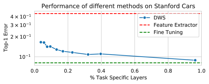
Figure 2: Accuracy vs Task Specific Layers: Accuracy vs percentage of task specific layers for the Cars dataset is shown. Varying $\lambda$ gives a variety of configuration. With even a very few task specific layers (high $\lambda$), we perform significantly better than the feature extraction baseline. Our method also reaches the fine-tune performance but needs a significant number of task specific layers.

Training details

We use an ImageNet pre-trained ResNet-50 [10] model as our base model for ImageNet-to-Sketch. We train TAPS for 30 epochs with batch size 32 on a single GPU. For the fine-tuning paragon and fixed feature extractor we report the best performance for the learning rates $lr\in\{0.001,0.005\}$.

For TAPS use the SGD optimizer with no weight decay. We sweep over $\lambda\in\{0.25,0.5,0.75\}$ and $lr\in\{0.001,0.005\}$. We fix the threshold, $\tau=0.1$, for all datasets and use the cosine annealing learning rate scheduler.

In addition to ResNet-50, we also apply TAPS to DenseNet-121 [11] and Vision Transformers [5]. To the best of our knowledge, we are the first to provide results for a transformer based architecture. The details of the training for these settings can be found in the B.1.

For the Visual Decathlon challenge, we use the WideResNet-28 as in [34], which is also referred to as ResNet-26 in [9]. Following existing work, we use a learning rate of 0.1 with weight decay of 0.0005 and train the network for 120 epochs. We report our results for $\lambda\in\{0.25,0.5,1.0\}$. Like existing methods [9, 34, 35], we report our accuracy on the test set while training on the training and validation dataset. We also calculate the $S$-Score to make a consolidated ranking of our method.

Results on ImageNet-to-Sketch

Tab. 1 shows the comparison of our method with existing approaches on ImageNet-to-Sketch. Average accuracy over 3 runs of our method and fine-tuning are reported. TAPS outperforms Piggyback and Packnet across all 5 datasets, Spot-Tune for 3 out of the 5 datasets, WTPB and BA² for 4 out of 5 datasets. We also note that TAPS uses, on average, only 57% of the parameters that Spot-Tune does. We do not outperform existing methods on the Cars dataset. Indeed, for this dataset the best results are obtained with $\lambda=0.0$ (see Fig. 2), suggesting that most layers needs to be adapted for optimal performance. We report the number of parameters used for each task in appendix C.2. In general, we perform significantly better in terms of accuracy compared to methods that are parameter efficient, while we achieve the same performance as methods that are designed for accuracy, but at a fraction of the parameter cost.

Table 1: Performance of various method using a ResNet-50 model on ImageNet-to-Sketch benchmark. Accuracy for different methods are shown for the different datasets. For TAPS and fine-tuning, we report the average accuracy over three runs. We report the total number of paramters (when available) and in parenthesis the data-type normalized parameter count. Numbers in bold denote the best performing method (other than fine-tuning) for each dataset. For Packnet, the arrow indicates the order of adding tasks.

	Param Count	Flowers	WikiArt	Sketch	Cars	CUB
Fine-Tuning	6$\times$	95.73	78.02	81.83	91.89	83.61
Feature Extractor	1$\times$	89.14	61.74	65.90	55.52	63.46
Piggyback [23]	6$\times$ (2.25$\times$)	94.76	71.33	79.91	89.62	81.59
Packnet [24] $\rightarrow$	(1.60$\times$)	93.00	69.40	76.20	86.10	80.40
Packnet [24] $\leftarrow$	(1.60$\times$)	90.60	70.3	78.7	80.0	71.4
Spot-tune [9]	7$\times$ (7$\times$)	96.34	75.77	80.2	92.4	84.03
WTPB [25]	6$\times$ (2.25$\times$)	96.50	74.8	80.2	91.5	82.6
BA2 [2]	3.8$\times$ (1.71$\times$)	95.74	72.32	79.28	92.14	81.19
TAPS	4.12$\times$	96.68	76.94	80.74	89.76	82.65

Table 2: Percentage of additional parameters and layers. The percentage of task specific parameters and layers needed for each dataset across network architectures is shown. Numbers in bold denote the lowest across architectures. ViT-S/16 uses the least number of extra parameters, while ResNet-50 adds the least number of task specific layers.

	Flowers	WikiArt	Sketch	Cars	CUB
Percentage of Additional Parameters
DenseNet-121	80.2	41.2	58.5	50.4	43.8
ViT-S/16	41.3	30.4	24.1	26.1	41.3
ResNet-50	65.5	52.8	75.9	41.9	70.6
Percentage of Task Specific Layers
DenseNet-121	69.4	22.5	41.1	28.3	23.9
ViT-S/16	54.2	20.8	22.9	37.5	54.2
ResNet-50	22.6	20.8	43.4	14.5	28.3

Task-specific layers

In Fig. 3, we show the layers that are task-specific for the different datasets. As expected, the final convolutional layers are always adapted. This corresponds to the common practice of freezing the initial 3 out of the 4 blocks of the ResNet-50 model and fine-tuning the last block. But, interestingly, we see that some of the middle layers are also always active. For instance, layer 26 is often adapted as a task-specific layer. Specifically for the Sketch task which has differing low-level features compared to ImageNet, the first convolution layer is consistently considered as task-specific. We see this is the case across varying values of $\lambda$, which aligns with the intuition that initial layers of ResNet should be retrained when transferring to a domain with different low-level features. A detailed figure of the task-specific layers for the Sketch task can be found in appendix 6.

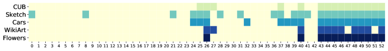
Figure 3: Task-specific layers for different datasets. Each row shows the 53 convolution layers of ResNet-50 layers for different datasets. Layer 0 is closest to the input, while layer 52 is closest to the classifier. Layers shown in yellow are shared with the ImageNet pre-trained model while layers shown in color are task-specific weights. We see that most tasks specific layers are toward the classifier.

Effect of choice of pre-trained model

To analyze the effect of using different pre-trained models, we replaced the base ImageNet model with a Places-365 model and applied TAPS on the datasets listed in Tab. 1. We notice changes both in task-specific layers and in the performance. The number of task-specific layers increases for every task, in particular the average percentage of task-specific layers grows from $25.91\%$ to $36.60\%$. We hypothesize that the Places-365 pre-training may not be well suited for object classification, so more layers need to be tuned. Supporting this, we also see a drop $2.77\%$ in average accuracy across the datasets (see 7 for details). These observations are consistent with the findings in [23].

Table 3: Accuracy of various methods across architectures and datasets. Classification accuracy for various methods is shown across different datasets and architectures. The ViT-S/16 model has the highest accuracy, across datasets. TAPS is able to match the fine-tuning performance for ViT-S/16 and is about 1-2% away for DenseNet-121.

	Flowers	WikiArt	Sketch	Cars	CUB
DenseNet-121
Fine-Tuning	95.6	77.0	81.1	89.5	82.6
Piggyback	94.7	70.4	79.7	89.1	80.5
TAPS	95.8	73.6	80.2	88.0	80.9
ViT-S/16
Fine-Tuning	99.3	82.6	81.9	89.2	88.9
TAPS	99.1	82.3	82.2	88.7	88.4

Effect of Architecture Choice

To demonstrate that TAPS is agnostic to architecture, we evaluate it on DenseNet-121 [11]. We report the performance of our method compared to fine-tuning and Piggyback in Tab. 3 and parameters in Tab. 2. The number of task-specific layers are high in DenseNet-121 compared to ResNet-50. We conjecture that because of the extra skip connections, changing a single layer has more impact on the output compared to the ResNet model.

Transformers

We show results of our method on the transformer architecture. Here, we use the ViT-S/16 model [45] (see B.1 for the training details). In Tab. 3 we report the performance of our method and parameters in Tab. 2. For the transformer architecture, the performance is better than CNNs as expected. We also notice that fewer parameters are made task-specific compared to CNNs. Although TAPS modifies more task specific layers, the adapted layers have fewer parameters. We show the layers that are task-specific in Fig. 4. From this figure we see that the layers that are adapted to be task-specific for transformers follow a very different pattern from those of CNNs. While in the latter, lower layers tend to be task agnostic, and final layers task-specific, this is not the case for transformers. Here, layers throughout the whole network tend to be adapted to the task. Moreover, attention and projection layers tend to be adapted, whereas MLP layers are fixed. This shows that TAPS can adapt in nontrivial ways to different architectures without any hand-crafted prior.

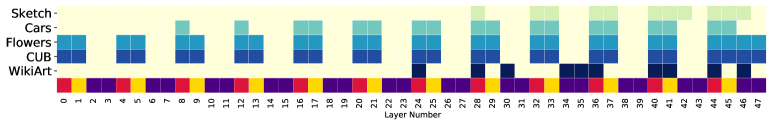
Figure 4: Task-specific layers for different datasets for the ViT model. The figure shows the task-specific layers that are active for different datasets. Each rows shows the different layers that are present in a ViT model. Layer 0 is closest to the input. Layers shown in yellow are shared with the ImageNet pre-trained model. The last row shows the type of layer and is denoted in color. Here crimson denotes the Query-Key-Value in the attention layer, gold denotes the projection layer and purple denotes the MLP layer. Unlike CNNs, we see that the fine-tuning strategy is very different. Instead of freezing blocks, we need to freeze the MLP layers.

Visual Decathlon

Tab. 4 shows that for $\lambda=0.25$, our method achieves the second highest S-score, without any dataset-specific hyper-parameter tuning. For this $\lambda$, we use half the number of parameters as Spot-Tune while performing better in 6/10 datasets and also have a higher mean score. All variants of our method outperform Res. Adapt., Deep Adapt., Piggyback. Moving from $\lambda=0.25$ to $\lambda=1.0$, we further reduce the number of task-specific layers by half while increasing the mean error only by $1\%$. At $\lambda=1$, we we outperform Piggyback while using lesser total number of parameters and storage space of the models, even considering that Piggyback uses Boolean parameters.

To analyze what layers are being used we plot the active layers at the highest compression $(\lambda=1)$ in Fig. 5. For all datasets, the number of task-specific layers is small, with Omniglot requiring the most layers, while DPed and GTSR require the least. In fact, for the latter datasets, no task-specific layers are required outside of updating the batch norm layers (which leads to a significant boost in performance compared to fixed feature extraction). Again, we note that TAPS can easily find complex nonstandard sharing schemes for each dataset, which would otherwise have required an expensive combinatorial search.

Table 4: Accuracy of various methods on the Visual Decathlon Challenge datasets. Accuracy for each dataset, the mean accuracy across all datasets and the S-Score [34] is shown. TAPS has the second best S-Score at almost half the parameters of the best method. Our method can tradeoff accuracy vs additional parameters. We report the total number of parameters and in parenthesis the data-type normalized parameter count.

Method	Params	Airc.	C100	DPed	DTD	GTSR	Flwr.	Oglt.	SVHN	UCF	Mean	S-Score
Fixed Feature [35]	1$\times$	23.3	63.1	80.3	45.4	68.2	73.7	58.5	43.5	26.8	54.3	544
FineTuning [35]	10$\times$	60.3	82.1	92.8	55.5	97.5	81.4	87.7	96.6	51.2	76.5	2500
Res. Adapt.[34]	2$\times$	56.7	81.2.	93.9	50.9	97.1	66.2	89.6	96.1	47.5	73.9	2118
DAM [37]	2.17$\times$	64.1	80.1	91.3	56.5	98.5	86.1	89.7	96.8	49.4	77.0	2851
PA [35]	2$\times$	64.2	81.9	94.7	58.8	99.4	84.7	89.2	96.5	50.9	78.1	3412
Piggyback[23]	10$\times$(3.25$\times$)	65.3	79.9	97.0	57.5	97.3	79.1	87.6	97.2	47.5	76.6	2838
WTPB [25]	10$\times$(3.25$\times$)	52.8	82.0	96.2	58.7	99.2	88.2	89.2	96.8	48.6	77.2	3497
BA2 [2]	6.13$\times$ (2.28$\times$)	49.9	78.1	95.5	55.1	99.4	86.1	88.7	96.9	50.2	75.7	3199
Spot-tune [9]	11$\times$	63.9	80.5	96.5	57.1	99.5	85.2	88.8	96.7	52.3	78.1	3612
TAPS ($\lambda$=0.25)	5.24$\times$	66.58	81.76	97.07	58.83	99.07	86.99	88.79	95.72	51.92	78.70	3533
TAPS ($\lambda$=0.50)	3.88$\times$	62.05	81.74	97.13	57.02	98.40	85.80	88.96	95.62	49.06	77.61	3180
TAPS ($\lambda$=0.75)	3.43$\times$	62.62	81.07	95.77	57.34	98.61	85.67	89.00	95.65	49.56	77.56	3096
TAPS ($\lambda$=1.0)	3.13$\times$	63.43	81.04	96.99	58.19	98.38	84.08	89.16	94.99	51.10	77.77	3088

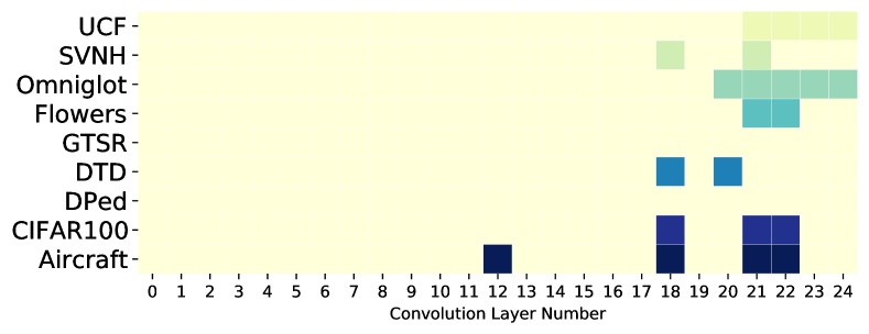
Figure 5: Task-specific layers for Visual Decathalon. Each row shows the task-specific layers for different datasets ($\lambda=1.0$). For two datasets: DPed and GTSR, no task-specific parameters are needed. The performance improves solely due to updating the batch norm parameters.

4.2 Joint Multi-Task Learning

Table 5: TAPS vs AdaShare. The accuracy of methods on the DomainNet dataset in both joint and incremental MTL settings is shown. All results are obtained with ResNet-34 unless stated otherwise. Bold numbers represent the higher accuracy between TAPS and AdaShare. Numbers with underline denote the best performing method in each setting. TAPS outperforms AdaShare in both settings. The Params column measures the total parameters for supporting all tasks in comparison with the single base model.

MTL Setting	Method	Params	Real	Painting	Quickdraw	Clipart	Infograph	Sketch	Mean
Joint	Fine-tuning	1$\times$	75.01	66.13	54.72	75.00	36.35	65.55	62.12
	AdaShare	1$\times$	76.90	67.90	61.17	75.88	31.52	63.96	62.88
	TAPS	1.46$\times$	78.91	67.91	70.18	76.98	39.30	67.81	66.84
Incremental	Fine-tuning	6$\times$	81.51	69.90	73.17	74.08	40.38	67.39	67.73
	AdaShare	5.73$\times$	79.39	65.74	68.15	74.45	34.11	64.15	64.33
	AdaShare ResNet-50	4.99$\times$	78.71	64.01	67.00	73.07	31.19	63.40	62.90
	TAPS	4.90$\times$	80.28	67.28	71.79	74.85	38.21	66.66	66.51

Setting

We compare TAPS with AdaShare [46] in the joint MTL setting, where multiple tasks are learned together with (selectively) shared backbones and independent task heads. We follow the same setting as AdaShare, i.e., datasets and network for a fair comparison. Specifically, we compare performance on the DomainNet datasets [31] with ResNet-34. This dataset contains the same labels across 6 domains and is an excellent candidate for MTL learning as there are opportunities for sharing as well as task competition.

To analyze the difference between TAPS and AdaShare, we further compare them in the incremental MTL setting, where each task is learned independently ($K=1$). We also include full fine-tuning as a baseline. Detailed training settings can be found in the B.2.

Select-or-Skip vs Add-or-Not

As shown in Table 5, TAPS outperforms AdaShare in both the incremental and joint multi-task settings across all six domains. This may partly be due to AdaShare’s select-or-skip strategy, which effectively reduces the number of residual blocks of the network. TAPS, on the other hand, replaces layers with task-specific versions without altering the model capacity, which results in performance closer to full fine-tuning. To verify whether a larger network will improve AdaShare’s performance, we perform the same incremental experiment with ResNet-50. Surprisingly, AdaShare with ResNet-50 has a slightly lower performance than its ResNet-34 version, suggesting that capacity might not be a limiting issue for the method.

Incremental Training vs Joint Training

As shown in Table 5, full fine-tuning for each task often yields the best performance and significantly outperforms the joint fine-tuning version. This suggests that task competition exists among the domains and only one domain (ClipArt) benefits from the joint training. When Adashare is trained with the incremental setting, we also see an increase in performance compared to the joint fine-tuning version. However, both methods come at the cost of weights sharing among tasks and a linear increase of the total model size. For TAPS, we see the performance is relatively stable when switching from joint training to incremental training and is close to the performance of fine-tuning.

Parameter and Training Efficiency

In the incremental setting, TAPS is 18% more parameter efficient compared to Adashare while performs 2.18% better on average. In this setting, AdaShare modifies the weights of existing layers and no layers are shared across tasks. Parameter savings here come from skipped blocks. Conversely, in the joint MTL setting, AdaShare is more parameter efficient, as no new parameters are introduced. However, this leads to performance degradation. TAPS performs uniformly better while introducing 0.46$\times$ more task-specific parameters.

As for training efficiency, AdaShare learns the select-or-skip policy first, which optimizes both weights and policy scores alternatively. After the policy learning phase, multiple architectures are sampled and retrained to get the best performance. This two-phase learning process increases the training cost significantly in comparison with TAPS, which has very little overhead compared to standard fine-tuning.

5 Limitations

A limitation of TAPS is that tasks do not share task-specific layers with each other, i.e., new tasks either learn their own task-specific parameters or share with the pre-trained model. The joint training approach we propose mitigates this issue by learning parameters common to all tasks. However, tasks added incrementally still cannot share parameters with others. Retraining the network on all tasks becomes infeasible as the number of tasks grow. We leave this aspect of parameter sharing as future work.

6 Conclusion

We have presented Task Adaptive Parameter Sharing, a simple method to adapt a base model to a new task by modifying a small task-specific subset of layers. We show that we are able to learn which layers to share differentiably using a straight-through estimator with gating over task-specific weight deltas. Our experimental results show that, TAPS retains high accuracy on target tasks using task-specific parameters. TAPS is agnostic to the particular architecture used, as seen in our results with ResNet-50, ResNet-34, DenseNet-121 and ViT models. We are able to discover standard and unique fine-tuning schemes. Furthermore, in the MTL setting we are able to avoid task competition by using task-specific weights.

In this supplementary material, we present additional details that we have referred to in the main paper.

Appendix A Datasets

ImageNet to Sketch Dataset

Originally introduced in [23] and referred to as Imagenet to Sketch in [2], our first benchmark consists of 5 datasets namely: CUB[48], Cars[15], WikiArt[42], Flowers[30] and Sketch[7]. Following [24], Cars and CUB are the cropped datasets, while the rest of the datasets are as is. For the Flowers dataset, we combine both the train and validation split as the training data. We resize all images to 256 and use a random resized crop of size 224 followed by a random horizontal flip. This augmentation is applied at training time to all the datasets except Cars and CUB. For these two datasets, we use only the horizontal flip as the data augmentation during training as in [24, 23, 9].

The Sketch dataset is licensed under a Creative Commons Attribution 4.0 International License. The CUBs, WikiArt, and Cars datasets use are restricted to non-commercial research and educational purposes.

Visual Decathlon Challenge

The Visual Decathlon Challenge [34] aims at evaluating visual recognition algorithms on images from multiple visual domains. The challenge consists of 10 datasets: ImageNet [39], Aircraft [22], CIFAR-100 [16], Describable textures [4], Daimler pedestrian classification [28], German traffic signs [44], UCF-101 Dynamic Images [43], SVHN [29], Omniglot [17], and Oxford Flowers [30]. The images of the Visual Decathlon datasets are resized isotropically to have a shorter side of 72 pixels, to alleviate the computational burden for evaluation. Each dataset has a different augmentation for training. We follow the training protocol as used in [34, 35]. Visual Decathlon does not explicitly provide a usage license.

DomainNet

DomainNet [31] is a benchmark for multi-source domain adaptation in object recognition. It contains 0.6M images across six domains (Clipart, Infograph, Painting, Quickdraw, Real, Sketch). All domains include 345 categories (classes) of objects. Each domain is considered as a task and we use the official train/test splits in our experiments. We also use the same augmentations as used in [46]. DomainNet is distributed under fair usage as provided for in section 107 of the US Copyright Law.

Appendix B Detailed Experimental Settings

B.1 Incremental MTL

As mentioned in the main paper, we describe detailed settings for all the experiments in Sec 4.1.

DenseNet-121 Training

We sweep through learning rate of $\{0.005,0.01\}$ and use a similar setup to our ResNet-50 model, i.e. SGD optimizer with no weight decay. We train for 30 epochs and use a cosine annealing learning rate scheduler. We used the same augmentation as that of ResNet-50 model as stated earlier. To summarize, the learning rate and the network architecture are the only things that change compared to the ResNet-50 model training.

ViT-S/16 Training

We train the ViT-S/16 model with a learning rate of 0.00005, momentum of 0.9, and $\lambda=1$. We train for 30 epochs with batch size of 32 and cosine annealing learning rate. Data augmentation consists of random resized crop and horizontal flip.

B.2 Joint MTL

In this section, we describe detailed settings for the DomainNet experiments in Sec 4.2. For each of the methods, we provide details regarding both joint and incremental MTL settings.

Fine-tuning

For the joint MTL setting, fine-tuning is done with the adjustment of batch size and learning rate. The shared backbone is trained with a batch size of 72 with 12 images from each task, learning rate 0.005, momentum 0.9, and no weight decay. We train for 60 epochs where an epoch consists of sampling every image across all 6 datasets. We find that balanced sampling over all tasks for each mini-batch is necessary for stable training as in [46].

For the incremental MTL setting, we train 30 epochs with batch size 32, learning rate 0.005, momentum 0.9, and weight decay 0.0001.

AdaShare

The learning process of AdaShare consists of two phases: the policy learning phase and retraining phase. During the policy learning phase, both weights and policies are optimized alternatively for 20K iterations. After the policy learning phase, different architectures are sampled with different seeds and the best results are reported. For the joint MTL setting, we follow the same setting as the original implementation [46]. Note that the original implementation samples 8 architectures from the learned policy and retrains them and report the best result, here for fair comparison with other methods, only 1 sampling is performed. For the incremental setting, we use the same setting as the joint-MTL, except the dataset contains only 1 domain.

TAPS

For all experiments we use learning rate 0.005, momentum 0.9, no weight decay, and $\lambda=1$. Data augmentation consists of a random resized crop and horizontal flip. For both the joint and incremental setting we train with a batch size of 32 and 30 epochs. The difference being for the joint variant we report in the main paper we start with the jointly trained backbone then train with the incremental variant of TAPS as opposed to an generic model for incremental training. When we use the joint version in which the backbone is trained simultaneously with the weight deltas, we train with batch size 72 and sample 12 images per task for each batch for 60 epochs.

Appendix C Additional Results

C.1 Imagenet to Sketch Benchmark

Amount of Additional Parameters

Flowers	WikiArt	Sketch	Cars	CUB
% Addl. Params.
65.50	52.82	75.87	41.85	70.61

Table 6: Additional parameters for ResNet-50 model on ImageNet-to-Sketch benchmark. Amount of Additional parameters (percentage) for TAPS are shown for the different datasets.

Tab. 6 shows the percentage of additional parameters needed for each dataset of this benchmark. In total we use about $4.12\times$ the number of parameters, with Cars using the least parameters and Sketch using the most.

Layers active for the Sketch dataset for various $\lambda$

We show in Fig. 6, the layers that are active for various values of $\lambda$ for the Sketch dataset. From this figure, we see that the first layer is task specific across different values of $\lambda$. This shows that the first layer is crucial for fine-tuning. This intuitively makes sense as the Sketch dataset has very different low level statistics compared to ImageNet.

Figure 6: When do we use task specific weights?. The plot shows the different task specific layers for the a model trained on the Sketch dataset. Each row represents the value of $\lambda$ for which the network uses task specific weights. Blue boxes indicate task specific layers while yellow boxes indicate base model layers. From this figure we can see that the lowest layers are active for any value of $\lambda$. Most other lower layers are turned off when $\lambda>0$

Effect of Pretraining on number of Task specific Parameters

	Flowers	WikiArt	Sketch	Cars	CUB
Resnet - 50
% Addl. Parameters
Imagenet	65.50	52.82	75.87	41.85	70.61
Places	75.08	68.72	74.59	75.02	74.72
% Task Specific Layers
Imagenet	22.64	20.75	43.40	14.47	28.30
Places	35.85	28.30	50.94	33.96	33.96

Table 7: Effect of Pretrained Model on Task specific parameters. Amount of parameters that are additionally needed for each task. The comparison between Imagenet pretrained model and Places pretrained model is shown. Across the board we see that the Places pretrained model uses more parameters as well as layers.

Show in Tab. 7 is the number of task specific layers and parameters that are needed for each dataset. From this table, we see that for all datasets the number of layers that are tasks specific are more for Places pretraining compared to an Imagenet pretraining. One could attribute this to the fact that the Places model specializes in scenes whereas the Imagenet model in objects. Hence, the Imagenet model is ”closer” to the tasks as opposed to the Places model.

Layers active for DenseNet-121

Fig. 7 shows the layers that are active for the DenseNet-121 model. From this figure we see that the number of layers that are task specific are much greater compared to the ResNet-50 model. Our hypothesis is that since DenseNet-121 has more skip connections, changing a layer has an effect on more layers as compared to ResNet-50.

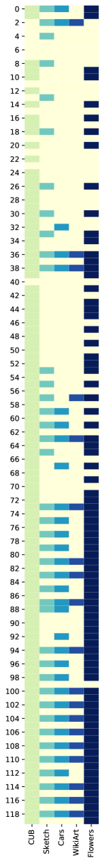
Figure 7: Shared layers for different tasks. The figure shows the task specific layers that are active for different datasets using a DenseNet-121 model. We observe that compared to the ResNet-50 model, many more layers are active for the same dataset.

C.2 Visual Decathalon

Method	Airc.	C100	DPed	DTD	GTSR	Flwr.	Oglt.	SVHN	UCF	Mean.	S-Score
TAPS($\lambda$=1.0)	63.43	81.04	96.99	58.19	98.38	84.08	89.16	94.99	51.10	77.77	3088
% Addl. Parameters	32.95	30.43	0.13	20.38	0.13	20.33	47.45	20.41	40.53
% Task specifc layer	16.00	12.00	0.00	8.00	0.00	8.00	20.00	8.00	16.00
TAPS( ($\lambda$=0.25)	66.58	81.76	97.07	58.83	99.07	86.99	88.79	95.72	51.92	78.703	3532
% Addl. Parameters	80.92	60.73	0.13	53.28	20.38	40.53	66.38	40.69	60.72
% Task specific layer	44.00	24.00	0.00	24.00	8.00	16.00	28.00	16.00	24.00

Table 8: Visual Decathalon additional parameter count. Shown in this table is the percentage of task specific layers as well as parameters needed for each task in addition to the base model. We show this for $\lambda=1.0$ and $\lambda=0.25$

In Tab. 8, we show the percentage of task specific layers as well as parameters for $\lambda=1.0$ and $\lambda=0.25$. From this table we see that as $\lambda$ increases, the percentage of task specific layers and parameters decreases. For the datasets where there are no task specific layers, the increase in parameters is due to the storage of batch norm parameters.

We also show the layers where task specific adaptation is needed for different values of $\lambda$ for the Visual Decathlon dataset. This can be seen in Fig. 8 $(\lambda=0.25)$, Fig. 9 $(\lambda=0.5)$, Fig. 10 $(\lambda=0.75)$ and Fig. 11 $(\lambda=1.0)$. For all the different values of $\lambda$, we see that almost all of the layers below layer 9 are not adapted. For the Aircraft dataset, layer 12 is consistently adapted. Similarly for the DTD dataset we consistently observe that no layers are adapted. This shows that some adaptations are independent of $lambda$ and hence critical for the task.

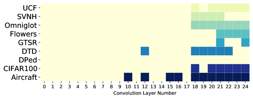
Figure 8: Task specific layers for different tasks. The figure shows the task specific layers that are adapted for different datasets in the Visual Decathlon challenge for $\lambda=0.25$

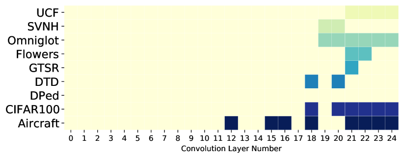
Figure 9: Task specific layers for different tasks. The figure shows the task specific layers that are adapted for different datasets in the Visual Decathlon challenge for $\lambda=0.50$

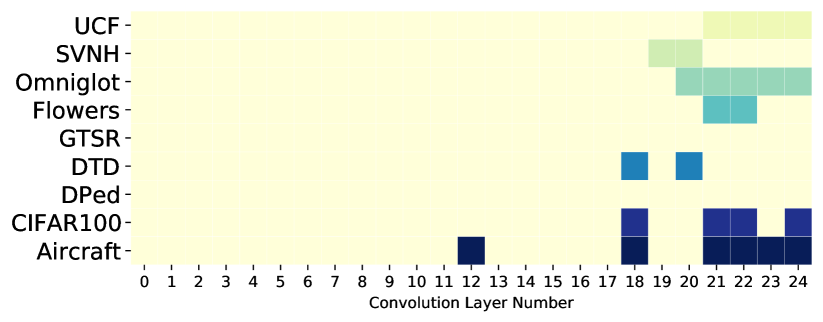
Figure 10: Task specific layers for different tasks. The figure shows the task specific layers that are adapted for different datasets in the Visual Decathlon challenge for $\lambda=0.75$

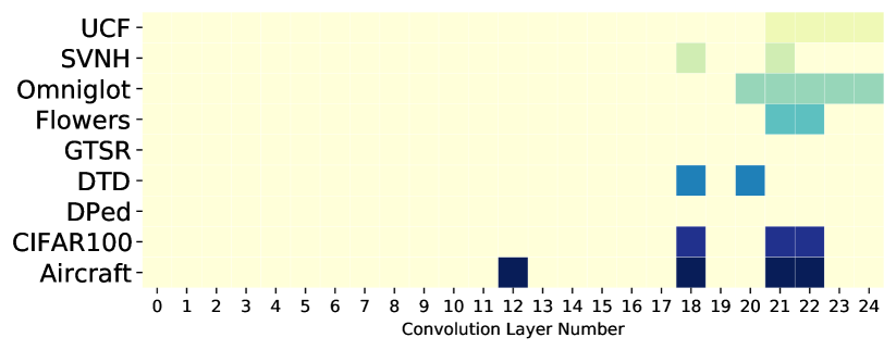
Figure 11: Task specific layers for different tasks. The figure shows the task specific layers that are adapted for different datasets in the Visual Decathlon challenge for $\lambda=1.0$

Appendix D Memory Efficient Joint Variant

See table 9 for comparison between the memory efficient variant and standard TAPS on the DomainNet benchmark for joint multi-task learning.

Method	Params	Real	Painting	Quickdraw	Clipart	Infograph	Sketch	Mean
TAPS (Standard)	1.43$\times$	78.45	68.23	70.32	77.00	39.35	67.95	66.88
TAPS (Mem. Efficient)	1.46$\times$	78.91	67.91	70.18	76.98	39.30	67.81	66.84

Table 9: Comparison between the memory efficient and standard version of TAPS on DomainNet in the joint MTL setting. The memory efficient version performs comparably in accuracy and parameter cost while only needing constant memory during training.

Appendix E Batch Norm and Manual Freezing

In Tab. 10 we report the results of only changing batch norm parameters and manually freezing layers to match the parameter cost of TAPS. We find that adaptively modifying layers outperforms manual freezing.

Appendix F PyTorch Implementation

We show the code snippet of a PyTorch implementation of TAPS in Algorithm 1 and Algorithm 2. The AdaptiveConv conv layers can be used to replace the normal Conv2d layers in an existing model. This shows how easily existing architectures can be used for training TAPS.

Algorithm 1 Pytorch Code for Gating Function with Straight Through Estimator

⬇

class BinarizeIndictator(autograd.Function):

@staticmethod

def forward(ctx, indicator, threshold=0.1):

out = (indicator >= threshold).float()

return out

@staticmethod

def backward(ctx, g):

# send the gradient g straight-through on the backward pass.

return g, None

Algorithm 2 Pytorch Code for Incremental Version of Task-Adaptive Convolutional Layers

⬇

class AdaptiveConv(nn.Conv2d):

def __init__(self, *args, **kwargs):

super().__init__(initial_val, *args, **kwargs)

weight_shape = self.weight.shape

#Initialize residual weights and indicator scores.

self.residual = torch.nn.Parameter(torch.zeros(weight_shape))

self.indicator = torch.nn.Parameter(torch.ones([initial_val])

#Freeze base network weights

self.weight.requires_grad = False

self.weight.grad = None

def forward(self, x):

I = BinarizeIndictator.apply(self.indicator)

w = self.weight + I * self.residual

x = F.conv2d(x, w)

return x

	Param	Flowers	WikiArt	Sketch	Cars	CUB
Feat. Extractor	1$\times$	89.14	61.74	65.90	55.52	63.46
BN	1.01$\times$	91.07	70.06	78.47	79.41	76.25
Man. Freeze	4.15$\times$	92.35	73.32	78.68	87.62	81.01
TAPS	4.12$\times$	96.68	76.94	80.74	89.76	82.65

Table 10: Performance of manually freezing layers and only adapting the batch norm parameters with a ResNet-50  model on ImageNet-to-Sketch benchmark. We observe that adapatively selecting which layers to modify with TAPS outperforms manually freezing an equivalent number of parameters starting from the last layers.

References

- [1] Yoshua Bengio, Nicholas Léonard, and Aaron Courville. Estimating or propagating gradients through stochastic neurons for conditional computation. arXiv preprint arXiv:1308.3432, 2013.
- [2] Rodrigo Berriel, Stephane Lathuillere, Moin Nabi, Tassilo Klein, Thiago Oliveira-Santos, Nicu Sebe, and Elisa Ricci. Budget-aware adapters for multi-domain learning. In Proceedings of the IEEE/CVF International Conference on Computer Vision (ICCV), October 2019.
- [3] Arslan Chaudhry, Marc’Aurelio Ranzato, Marcus Rohrbach, and Mohamed Elhoseiny. Efficient lifelong learning with a-gem. In ICLR, 2019.
- [4] M. Cimpoi, S. Maji, I. Kokkinos, S. Mohamed, , and A. Vedaldi. Describing textures in the wild. In Proceedings of the IEEE Conf. on Computer Vision and Pattern Recognition (CVPR), 2014.
- [5] Alexey Dosovitskiy, Lucas Beyer, Alexander Kolesnikov, Dirk Weissenborn, Xiaohua Zhai, Thomas Unterthiner, Mostafa Dehghani, Matthias Minderer, Georg Heigold, Sylvain Gelly, Jakob Uszkoreit, and Neil Houlsby. An image is worth 16x16 words: Transformers for image recognition at scale, 2020.
- [6] Mathias Eitz, James Hays, and Marc Alexa. How do humans sketch objects? ACM Transactions on Graphics (TOG), 31:1 – 10, 2012.
- [7] Mathias Eitz, James Hays, and Marc Alexa. How do humans sketch objects? ACM Trans. Graph. (Proc. SIGGRAPH), 31(4):44:1–44:10, 2012.
- [8] Yuan Gao, Jiayi Ma, Mingbo Zhao, Wei Liu, and Alan L Yuille. Nddr-cnn: Layerwise feature fusing in multi-task cnns by neural discriminative dimensionality reduction. In Proceedings of the IEEE/CVF Conference on Computer Vision and Pattern Recognition, pages 3205–3214, 2019.
- [9] Yunhui Guo, Honghui Shi, Abhishek Kumar, Kristen Grauman, Tajana Rosing, and Rogerio Feris. Spottune: transfer learning through adaptive fine-tuning. In Proceedings of the IEEE/CVF Conference on Computer Vision and Pattern Recognition, pages 4805–4814, 2019.
- [10] Kaiming He, X. Zhang, Shaoqing Ren, and Jian Sun. Deep residual learning for image recognition. 2016 IEEE Conference on Computer Vision and Pattern Recognition (CVPR), pages 770–778, 2016.
- [11] Gao Huang, Zhuang Liu, Laurens van der Maaten, and Kilian Q Weinberger. Densely connected convolutional networks. In Proceedings of the IEEE Conference on Computer Vision and Pattern Recognition, 2017.
- [12] Eric Jang, Shixiang Gu, and Ben Poole. Categorical reparameterization with gumbel-softmax. arXiv preprint arXiv:1611.01144, 2016.
- [13] James Kirkpatrick, Razvan Pascanu, Neil Rabinowitz, Joel Veness, Guillaume Desjardins, Andrei A. Rusu, Kieran Milan, John Quan, Tiago Ramalho, Agnieszka Grabska-Barwinska, Demis Hassabis, Claudia Clopath, Dharshan Kumaran, and Raia Hadsell. Overcoming catastrophic forgetting in neural networks. Proceedings of the National Academy of Sciences, 114(13):3521–3526, 2017.
- [14] Iasonas Kokkinos. Ubernet: Training a universal convolutional neural network for low-, mid-, and high-level vision using diverse datasets and limited memory. In CVPR, pages 6129–6138, 2017.
- [15] Jonathan Krause, Michael Stark, Jia Deng, and Li Fei-Fei. 3d object representations for fine-grained categorization. 2013 IEEE International Conference on Computer Vision Workshops, pages 554–561, 2013.
- [16] Alex Krizhevsky, Geoffrey Hinton, et al. Learning multiple layers of features from tiny images. 2009.
- [17] Brenden M Lake, Ruslan Salakhutdinov, and Joshua B Tenenbaum. Human-level concept learning through probabilistic program induction. Science, 350(6266):1332–1338, 2015.
- [18] Yanghao Li, Naiyan Wang, Jianping Shi, Jiaying Liu, and Xiaodi Hou. Revisiting batch normalization for practical domain adaptation. arXiv preprint arXiv:1603.04779, 2016.
- [19] Zhizhong Li and Derek Hoiem. Learning without forgetting. IEEE transactions on pattern analysis and machine intelligence, 40(12):2935–2947, 2017.
- [20] Yongxi Lu, Abhishek Kumar, Shuangfei Zhai, Yu Cheng, Tara Javidi, and Rogerio Feris. Fully-adaptive feature sharing in multi-task networks with applications in person attribute classification. In Proceedings of the IEEE conference on computer vision and pattern recognition, pages 5334–5343, 2017.
- [21] Chris J Maddison, Andriy Mnih, and Yee Whye Teh. The concrete distribution: A continuous relaxation of discrete random variables. arXiv preprint arXiv:1611.00712, 2016.
- [22] S. Maji, J. Kannala, E. Rahtu, M. Blaschko, and A. Vedaldi. Fine-grained visual classification of aircraft. Technical report, 2013.
- [23] Arun Mallya, Dillon Davis, and Svetlana Lazebnik. Piggyback: Adapting a single network to multiple tasks by learning to mask weights. In Proceedings of the European Conference on Computer Vision (ECCV), pages 67–82, 2018.
- [24] Arun Mallya and Svetlana Lazebnik. Packnet: Adding multiple tasks to a single network by iterative pruning. In Proceedings of the IEEE conference on Computer Vision and Pattern Recognition, pages 7765–7773, 2018.
- [25] Massimilano Mancini, Elisa Ricci, Barbara Caputo, and Samuel Rota Bulò. Adding new tasks to a single network with weight transformations using binary masks. In Proceedings of the European Conference on Computer Vision (ECCV) Workshops, September 2018.
- [26] Ishan Misra, Abhinav Shrivastava, Abhinav Gupta, and Martial Hebert. Cross-stitch networks for multi-task learning. In Proceedings of the IEEE conference on computer vision and pattern recognition, pages 3994–4003, 2016.
- [27] Pedro Morgado and Nuno Vasconcelos. Nettailor: Tuning the architecture, not just the weights. In Proceedings of the IEEE/CVF Conference on Computer Vision and Pattern Recognition, pages 3044–3054, 2019.
- [28] Stefan Munder and Dariu M Gavrila. An experimental study on pedestrian classification. IEEE transactions on pattern analysis and machine intelligence, 28(11):1863–1868, 2006.
- [29] Yuval Netzer, Tao Wang, Adam Coates, Alessandro Bissacco, Bo Wu, and Andrew Y Ng. Reading digits in natural images with unsupervised feature learning. 2011.
- [30] Maria-Elena Nilsback and Andrew Zisserman. Automated flower classification over a large number of classes. 2008 Sixth Indian Conference on Computer Vision, Graphics & Image Processing, pages 722–729, 2008.
- [31] Xingchao Peng, Qinxun Bai, Xide Xia, Zijun Huang, Kate Saenko, and Bo Wang. Moment matching for multi-source domain adaptation. In Proceedings of the IEEE/CVF International Conference on Computer Vision, pages 1406–1415, 2019.
- [32] Rajeev Ranjan, Vishal M Patel, and Rama Chellappa. Hyperface: A deep multi-task learning framework for face detection, landmark localization, pose estimation, and gender recognition. IEEE transactions on pattern analysis and machine intelligence, 41(1):121–135, 2017.
- [33] Mohammad Rastegari, Vicente Ordonez, Joseph Redmon, and Ali Farhadi. Xnor-net: Imagenet classification using binary convolutional neural networks. In European conference on computer vision, pages 525–542. Springer, 2016.
- [34] Sylvestre-Alvise Rebuffi, Hakan Bilen, and Andrea Vedaldi. Learning multiple visual domains with residual adapters. arXiv preprint arXiv:1705.08045, 2017.
- [35] Sylvestre-Alvise Rebuffi, Hakan Bilen, and Andrea Vedaldi. Efficient parametrization of multi-domain deep neural networks. In Proceedings of the IEEE Conference on Computer Vision and Pattern Recognition, pages 8119–8127, 2018.
- [36] Sylvestre-Alvise Rebuffi, Alexander Kolesnikov, Georg Sperl, and Christoph H. Lampert. icarl: Incremental classifier and representation learning. In 2017 IEEE Conference on Computer Vision and Pattern Recognition (CVPR), pages 5533–5542, 2017.
- [37] Amir Rosenfeld and John K Tsotsos. Incremental learning through deep adaptation. IEEE transactions on pattern analysis and machine intelligence, 42(3):651–663, 2018.
- [38] Sebastian Ruder, Joachim Bingel, Isabelle Augenstein, and Anders Søgaard. Latent multi-task architecture learning. In Proceedings of the AAAI Conference on Artificial Intelligence, volume 33, pages 4822–4829, 2019.
- [39] Olga Russakovsky, Jia Deng, Hao Su, Jonathan Krause, Sanjeev Satheesh, Sean Ma, Zhiheng Huang, Andrej Karpathy, Aditya Khosla, Michael S. Bernstein, Alexander C. Berg, and Li Fei-Fei. Imagenet large scale visual recognition challenge. International Journal of Computer Vision, 115:211–252, 2015.
- [40] Andrei A. Rusu, Neil C. Rabinowitz, Guillaume Desjardins, Hubert Soyer, James Kirkpatrick, Koray Kavukcuoglu, Razvan Pascanu, and Raia Hadsell. Progressive neural networks. ArXiv, abs/1606.04671, 2016.
- [41] Babak Saleh and A. Elgammal. Large-scale classification of fine-art paintings: Learning the right metric on the right feature. ArXiv, abs/1505.00855, 2015.
- [42] Babak Saleh and Ahmed Elgammal. Large-scale classification of fine-art paintings: Learning the right metric on the right feature. arXiv preprint arXiv:1505.00855, 2015.
- [43] Khurram Soomro, Amir Roshan Zamir, and Mubarak Shah. Ucf101: A dataset of 101 human actions classes from videos in the wild. arXiv preprint arXiv:1212.0402, 2012.
- [44] Johannes Stallkamp, Marc Schlipsing, Jan Salmen, and Christian Igel. Man vs. computer: Benchmarking machine learning algorithms for traffic sign recognition. Neural networks, 32:323–332, 2012.
- [45] Andreas Steiner, Alexander Kolesnikov, Xiaohua Zhai, Ross Wightman, Jakob Uszkoreit, and Lucas Beyer. How to train your vit? data, augmentation, and regularization in vision transformers. arXiv preprint arXiv:2106.10270, 2021.
- [46] Ximeng Sun, Rameswar Panda, Rogerio Feris, and Kate Saenko. Adashare: Learning what to share for efficient deep multi-task learning. Neural Information Processing Systems, 2020.
- [47] Simon Vandenhende, Stamatios Georgoulis, Bert De Brabandere, and Luc Van Gool. Branched multi-task networks: deciding what layers to share. arXiv preprint arXiv:1904.02920, 2019.
- [48] Catherine Wah, Steve Branson, Peter Welinder, Pietro Perona, and Serge J. Belongie. The caltech-ucsd birds-200-2011 dataset. 2011.
- [49] Mitchell Wortsman, Ali Farhadi, and Mohammad Rastegari. Discovering neural wirings. Advances in Neural Information Processing Systems, 32, 2019.
- [50] Jeffrey O Zhang, Alexander Sax, Amir Zamir, Leonidas Guibas, and Jitendra Malik. Side-tuning: A baseline for network adaptation via additive side networks. In Computer Vision–ECCV 2020: 16th European Conference, Glasgow, UK, August 23–28, 2020, Proceedings, Part III 16, pages 698–714. Springer, 2020.