Active Learning for Computationally Efficient Distribution of Binary Evolution Simulations

Abstract

Binary stars undergo a variety of interactions and evolutionary phases, critical for predicting and explaining observations. Binary population synthesis with full simulation of stellar structure and evolution is computationally expensive, requiring a large number of mass-transfer sequences. The recently developed binary population synthesis code POSYDON incorporates grids of MESA binary-star simulations that are interpolated to model large-scale populations of massive binaries. The traditional method of computing a high-density rectilinear grid of simulations is not scalable for higher-dimension grids, accounting for a range of metallicities, rotation and eccentricity. We present a new active learning algorithm, psy-cris, which uses machine learning in the data-gathering process to adaptively and iteratively target simulations to run, resulting in a custom, high-performance training set. We test psy-cris on a toy problem and find the resulting training sets require fewer simulations for accurate classification and regression than either regular or randomly sampled grids. We further apply psy-cris to the target problem of building a dynamic grid of MESA simulations, and we demonstrate that, even without fine tuning, a simulation set of only $\sim 1/4$ the size of a rectilinear grid is sufficient to achieve the same classification accuracy. We anticipate further gains when algorithmic parameters are optimized for the targeted application. We find that optimizing for classification only may lead to performance losses in regression, and vice versa. Lowering the computational cost of producing grids will enable new population synthesis codes such as POSYDON to cover more input parameters while preserving interpolation accuracies.

1 Introduction

Theoretical studies in astronomy often include simulations of physical processes that are not well constrained or understood with the purpose of making predictions and comparisons against observations. To account for model or physical uncertainties, simulations are carried out with various combinations of unconstrained parameters to explore the space of possible outcomes. However, in many cases, the computational cost per simulation is large and limits the exploration of the parameter space. For example, three-dimensional (3D) hydrodynamic supernova (SNe) simulations can take up to tens of millions of CPU-hours per simulation on current facilities (e.g., Müller et al., 2017; Vartanyan et al., 2019; Bollig et al., 2021). Large scale cosmological simulations such as those from the Illustris project performed with the AREPO code (Springel, 2010), demand similarly high computational costs (Nelson et al., 2018; Wang et al., 2021). Another area where large computational resources are expended is in modeling single and binary stars with one-dimensional (1D) stellar structure and evolution codes such as Modules for Experiments in Stellar Astrophysics (MESA; Paxton et al., 2011, 2013, 2015, 2018, 2019) especially when considering galactic populations. Large scale computing is not only a significant investment of time and financial resources, but also comes with a carbon footprint, hence optimization also minimizes our environmental impact (Portegies Zwart, 2020). In this work, we aim to reduce the cost of producing data sets of binary evolution simulations for large populations through active learning (AL).

Binary population synthesis (hereafter population synthesis) codes simulate large numbers of binary star systems and their interactions to compare their statistics against observations (e.g., Han et al., 2020). While population synthesis has broad applicability, there are large computational hurdles to overcome when modeling binary populations. Not only does one have to model complex physical processes like mass transfer, SNe and evolution, but one also needs to model large numbers ($10^{7}$–$10^{9}$) of systems since many astrophysically interesting phenomena are also rare . Therefore, the computational cost to model each binary must be low to evolve a reasonably sized population with tens of millions of systems. Given a population synthesis code, the number of binaries that need to be simulated to understand an astrophysical population may be reduced by using targeted sampling methods (e.g., Andrews et al., 2018; Broekgaarden et al., 2019); however, there can still be considerable computation cost associated with evolving a binary accurately. To address this computational challenge fitting formulae were developed to reproduce single star evolution (SSE) across a range of masses and metallicities (Hurley et al., 2000). The SSE equations were then combined with recipes to approximate the evolution of binary stars in the population synthesis code Binary Stellar Evolution (BSE; Hurley et al., 2002). This approach was computationally efficient enough for population studies, but came at the cost of physical approximations (e.g., simple parameterizations for the stability of mass transfer, lack of self-consistency in the treatment of stars out of thermal equilibrium and of stellar wind mass loss).

Since the development of Binary Stellar Evolution (BSE), similar rapid population synthesis codes have been developed using the same underlying methodology of relying on the SSE fitting formulae for single star evolution and different recipes to approximate binary evolution. These include , StarTrack (Belczynski et al., 2002, 2008), binary_c (Izzard et al., 2004, 2006, 2009), COMPAS (Stevenson et al., 2017; Barrett et al., 2018; Riley et al., 2022), MOBSE (Giacobbo et al., 2018), and COSMIC (Breivik et al., 2020). There are other approaches to population synthesis diverging from using SSE fitting formulae, aiming to increase the accuracy of physics being implemented. The ComBinE (Kruckow et al., 2018) and SEVN (Spera et al., 2015, 2019) codes use dense grids of single star evolutionary sequences and performs linear interpolation between models. BPASS provides more accurate modelling of stellar populations as it uses detailed binary models including their interactions although without simultaneously evolving both stars (Eldridge et al., 2017).

POpulation SYnthesis with Detailed binary-evolution simulatiONs (POSYDON) is a new population synthesis code that uses full detailed binary evolution simulations evolved with Modules for Experiments in Stellar Astrophysics (MESA) to perform population synthesis (Fragos et al., 2022).

Although a single 1D stellar evolution simulation may have a modest cost ranging from tens to hundreds of CPU-hours, it is common to compute thousands to tens of thousands of models due to the intrinsically large number of parameters that describe stellar and binary physics. (e.g., Fragos et al., 2015; Farmer et al., 2015; Choi et al., 2016; Misra et al., 2020; Marchant et al., 2021; Gallegos-Garcia et al., 2021; García et al., 2021; Román-Garza et al., 2021). Although the aforementioned studies show that MESA simulations can be scaled to run large numbers of systems, they are still too computationally expensive to directly model galactic populations.

The POSYDON framework uses large data sets of precomputed binary evolution simulations to evolve a population through various phases of evolution. To approximate the evolution of a binary system for which no precomputed model exists, interpolation is employed. To maximize the interpolation accuracy, and the subsequent population synthesis, the detailed binary simulations must cover an adequate range of parameter space to resolve complex behavior. Since binary stellar evolution has many intrinsic input parameters (e.g., component masses $M_{1}$, $M_{2}$, orbital period $P_{\mathrm{orb}}$, eccentricity $e$, metallicity $Z$), orders of magnitude more models compared to the single star approach of previous codes.

A common procedure for building these data sets is to choose the most important parameters in the problem and create a dense regular (rectilinear) grid of simulations. Then, the density is generally chosen based upon a combination of physical intuition about the problem and manual inspection (e.g., Wellstein & Langer, 1999; Nelson & Eggleton, 2001; de Mink et al., 2007; Farmer et al., 2015; Misra et al., 2020; Marchant et al., 2021). However, POSYDON data sets of binary simulations will have prohibitively large computational cost to produce when we consider expanding the dimensionality of our data sets. For example, to construct a grid of detailed binary simulations with 10 points in each of 5 dimensions, assuming a typical computation time of 12 hours per simulation, it would cost $1.2$ million CPU-hours to complete. We propose active learning as a solution for building grids of binary simulations, at a fraction of the cost of current methods of sampling parameter space.

AL is the process of intelligently sampling points of interest to build a custom training data set for machine learning (ML) algorithms (Settles, 2009). AL is useful in situations where labeling instances (e.g., running a simulation, human annotation of data) is expensive or the number of samples to label is large. Depending on the application, AL algorithms optimize for either classification or regression with applications including speech recognition, image classification, and information extraction (Kumar & Gupta, 2020). it has been proposed as a way to optimize spectroscopic follow-up for labeling supernovae light curves (Ishida et al., 2019; Kennamer et al., 2020), as well as mitigating sample selection bias for photometric classification of stars (Richards et al., 2012). It has also been applied to multiple computational astrophysics problems to build training sets for interpolation or increased performance over standard sampling methods (e.g., Solorio et al., 2005; Doctor et al., 2017; Ristic et al., 2022; Daningburg & O’Shaughnessy, 2022).

In this paper we present an AL framework for dynamically constructing data sets of binary simulations to be used in population synthesis codes such as POSYDON. In §2 we introduce our new AL algorithm, psy-cris (PoSYdon Classification and Regression Informed Sampling), and describe our implementation. Then we present two tests of psy-cris: first on a synthetic data set §3 and then in a real-world scenario using MESA to run binary evolution simulations §4. In §5 we discuss the results of our tests. We find that psy-cris performs well when optimized on synthetic data and we see promising performance when applying our method to construct a data set of MESA simulations. The psy-cris code is open source, and will be available as a module of POSYDON. The psy-cris algorithm is broadly applicable to other AL problems with both classification and regression data.

2 The psy-cris Algorithm

2.1 Defining the Problem

To describe the psy-cris algorithm, we first provide a description of the data set and the problem we are trying to solve in the context of binary population synthesis with POSYDON.

An individual simulation corresponds to a vector $\mathcal{S}_{\mathrm{}}(t)=[v_{1}(t),\dots,v_{n}(t)]$ that evolves in time $t$ based on some physical model $\mathbf{p}$. We can write the evolution of a simulation from an initial state $\mathcal{S}_{\mathrm{i}}$ to some final state $\mathcal{S}_{\mathrm{f}}$ with our model $\mathbf{p}$ as $\mathbf{p}{}(\mathcal{S}_{\mathrm{i}})=\mathcal{S}_{\mathrm{f}}=[v_{1}(t_{f}),\dots,v_{n}(t_{f})]$. Our task is to predict the outcomes of all simulations in a given simulation domain $D$, without manually running simulations at all points in the space due to the prohibitive computational cost.

In the case of POSYDON, $D$ would consist of parameters describing binary stellar evolution (e.g., component masses $M_{1}$ and $M_{2}$, orbital period $P_{\mathrm{orb}}$, metallicity $Z$, stellar rotation $\omega_{1}$ and $\omega_{2}$, eccentricity $e$). Our physical model $\mathbf{p}$ is MESA, evolving a binary system from some initial configuration to a final state. Then, $v(t)$ is anything reported by, or post-processed from the MESA simulations, that change over the evolution of a binary. For example, it could be a real number, like the mass of the star at time $t$, or it could be a classification, such as whether a star is a black hole (BH) or a neutron star (NS). In POSYDON, we use ML techniques to predict the outcomes of these MESA simulations to evolve a binary population through various phases of evolution.

It is helpful to split our domain into two categories: the set of labeled data $L_{\mathrm{}}$, completed simulations with inputs and outputs, and unlabeled data $U_{\mathrm{}}$, the space of possible simulations which have not been computed. To evolve simulations $\mathcal{S}_{\mathrm{i}}\in U_{\mathrm{}}$, we can use a ML model $\Gamma$ trained on a labeled data set $L_{\mathrm{}}$, denoted as $\Gamma{}_{L_{\mathrm{}}}$. Then the predicted evolution of a simulation is given by:

$$\Gamma{}_{L_{\mathrm{}}}(\mathcal{S}_{\mathrm{i}})=\mathcal{S}_{\mathrm{f}}^{*},$$ (1)

where the star in $\mathcal{S}_{\mathrm{f}}^{*}$ denotes predicted final properties. For many computational-astrophysics problems, the computational cost of evaluating $\Gamma{}_{L_{\mathrm{}}}(\mathcal{S}_{\mathrm{i}})$ is much less than $\mathbf{p}{}(\mathcal{S}_{\mathrm{i}})$. To be applicable in any scientific studies, we must also ensure that our ML model has high accuracy, i.e., $\mathcal{S}_{\mathrm{f}}^{*}\approx\mathcal{S}_{\mathrm{f}}$. However, we must also consider the cost of computing our training set $L_{\mathrm{}}$ and then optimizing $\Gamma$, each of which is not always negligible .

Our study focuses on identifying an optimal $L_{\mathrm{}}$, without knowing a priori what our simulations across $D$ may look like, at a minimized computational cost. Our AL algorithm psy-cris takes an initially sparse training data set $L_{\mathrm{}}$, and identifies new points $\mathcal{S}_{\mathrm{i}}\in U_{\mathrm{}}$ such that when they are labeled and added to the training set for $\Gamma$ , we achieve high accuracy ($\Gamma{}_{L_{\mathrm{}}}(\mathcal{S}_{\mathrm{i}})\approx\mathbf{p}{}(\mathcal{S}_{\mathrm{i}})$) with a low computational cost compared to standard methods of constructing the training set.

2.2 Algorithm & Workflow

AL algorithms take as input an initial training data set and output query points to be labeled by an oracle (Settles, 2009). The oracle may be a human manually labelling data or the results of simulations that we treat as the truth (as in POSYDON). AL algorithms work in a loop with the oracle to iteratively build a training data set designed to achieve high accuracy in interpolation with an economical number of simulations. It is common for AL algorithms to be applied in either classification or regression problems (Kumar & Gupta, 2020), but in POSYDON our data naturally span both regimes. For example, one can classify binary simulations using their mass transfer histories and perform regression on their continuous output quantities like final orbital separation, age, and component masses. Therefore, we designed psy-cris to consider both classification and regression simultaneously.

We achieve this by first combining AL heuristics, which are estimates for uncertainty in classification or regression (§2.3.2). Next, we sample from this new, combined AL heuristic and generate an uncertainty distribution (§2.3.3). Finally, we draw query points from the uncertainty distribution in serial or batches. This completes a single AL loop of psy-cris which will repeat until a termination condition is met. This condition can simply be a maximum number of sampled points, or something more complex. The details of the psy-cris algorithm are described in Section 2.3, our exact implementation is described in Section 2.4, and our results from applying psy-cris are presented in Section 3 and Section 4.

Figure 1 shows a schematic diagram of psy-cris integrated with POSYDON to run binary stellar evolution simulations with MESA. The green rectangle shows the scope of the psy-cris algorithm and how it integrates with other portions of POSYDON infrastructure. POSYDON runs binary simulations with MESA queried by psy-cris and then post-processes the output into our pre-defined classes and regression quantities. The blue square represents the oracle in an AL loop and can be replaced with other simulation software.

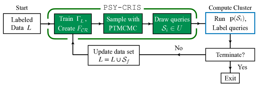
Figure 1: A schematic AL flowchart showing how psy-cris integrates with a compute cluster to submit and label MESA simulations using POSYDON infrastructure. In our case, $\mathbf{p}$ is MESA, but in general it may be switched out for any other simulation software. The loop starts from a set of labeled data $L_{\mathrm{}}$ given to psy-cris, which outputs a set of new query points $\mathcal{S}_{\mathrm{i}}$ to be labeled. The term $F_{\mathcal{CR}}$ is our custom AL heuristic which combines classification and regression simultaneously (Equation 2). After the queried MESA simulations complete, POSYDON post processes and labels the outcomes of each simulation ($\mathcal{S}_{\mathrm{f}}$). Then, the AL loop can continue by feeding the updated training set back into psy-cris, or it can terminate and exit. The final result after multiple iterations is a training data set $L_{\mathrm{AL}}$ designed to provide better performance for classification and regression algorithms compared to a simpler distribution of training data.

2.3 Components & Concepts

2.3.1 Classification & Regression AL Heuristics

Classification deals with categorical data while regression is used in cases where data are continuously valued. For example, we may classify a binary evolution simulation based on its mass transfer history while a regression quantity may be the final mass of each component. Conceptually, a classification or regression AL heuristic is designed to locate unlabeled samples of interest based on a given ML method applied to $L_{\mathrm{.}}$ If the ML algorithm has a measure of uncertainty in its predictions, or if one can be constructed, then this can be used as an AL heuristic. We denote a general classification or regression AL heuristics as $\mathcal{C}$ and $\mathcal{R}$ respectively.

2.3.2 Combining Classification & Regression AL Heuristics

We designed the psy-cris algorithm to optimize for both classification and regression simultaneously. To enable this coupled optimization, we propose that a linear combination of individual heuristics can also be used as a heuristic. We denote our new heuristic as $F_{\mathcal{CR}}$ defined as:

$$F_{\mathcal{CR}}(\mathbf{x})=\left[\tau F_{\mathcal{C}}(\mathbf{x})+(1-\tau)F_{\mathcal{R}}(\mathbf{x})\right]^{\beta}$$ (2)

where $\mathbf{x}$ is a point in parameter space, $\tau\in[0,1]$ sets the fractional contribution of the classification and regression terms, and $\beta$ controls the sharpness of the distribution (similarly to an inverse temperature; Mehrjou et al., 2018). The terms $F_{\mathcal{C}}$ and $F_{\mathcal{R}}$ are normalized heuristics. Since we combine $\mathcal{C}$ and $\mathcal{R}$ terms, their relative scaling matters. Equation 2 is designed to be high valued in regions with the largest estimated uncertainty in classification and regression.

2.3.3 Sampling Query Points

Once the heuristic has been defined, we must select query points for the oracle to label. AL algorithms can return either a single query point (serial) or a set of query points (batch) to label. Batch proposal schemes introduce more complexity, but allow multiple queries to be labeled in parallel. This may be less efficient in terms of the total number of simulations needed than only ever picking the best point, but provides a advantage in terms of computational wall time (Schohn & Cohn, 2000; Cai et al., 2017; Sener & Savarese, 2017; Kennamer et al., 2020). With batch proposals, we consider more than just the maximum of the AL heuristic, but also the diversity of samples in the batch to avoid redundancy (King et al., 2004; Hoi et al., 2006; Demir et al., 2011; Wang et al., 2017).

In psy-cris we adopt a flexible approach which allows either serial or batch proposals, by creating an uncertainty distribution from which any number of query points can be drawn. We use our combined heuristic in Equation 2 as the target distribution for a parallel tempered Markov-chain Monte Carlo (PTMCMC) sampling algorithm (Swendsen & Wang, 1986). We assume that psy-cris may query any point in the input space, and is not constrained to a fixed or discrete pool of unlabeled samples. Drawing query points is the final step in one psy-cris iteration.

2.4 Implementation

2.4.1 Classifiers & Regressors

We perform one-against-all binary classification. For data with $n$ classes (where $n>2$), we train $n$ binary classifiers and define the predicted class $\hat{y}$ and classification probability $P(\hat{y}|\mathbf{x})$ respectively

$$\hat{y}=\operatorname*{arg\,max}\limits_{i=1,\ldots,n}[\theta_{i}(\mathbf{x})],$$ (3)

$$P(\hat{y}|\mathbf{x})=\max\limits_{i=1,\ldots,n}[\theta_{i}(\mathbf{x})],$$ (4)

where $\mathbf{x}$ is a query point in parameter space and $\theta_{i}$ denotes a binary classifier for the $i$-th class. The classifier $\theta_{i}(\mathbf{x})$, returns the probability that a query point $\mathbf{x}$ corresponds to class $i$.

To construct our classification heuristic we use a least confident measure for classification (Lewis & Gale, 1994; Settles, 2009; Kumar & Gupta, 2020):

$$F_{\mathcal{C}}(\mathbf{x})=\frac{n}{n-1}\left(1-P(\hat{y}|\mathbf{x})\right),$$ (5)

where $\mathbf{x}$ is a query point, $n$ is the total number of classes in the data set, and $P(\hat{y}|\mathbf{x})$ is the classification probability in Equation 4. The prefactor is a pseudo-normalization term in the event all $n$ classes intersect at some point in the domain, which need not occur.

We train regression algorithms on data separated by class, taking into account both the different numbers of outputs and unique outputs per class. For $n$ classes that all have $m$ outputs, there are $n\times m$ interpolation algorithms trained.

For AL regression problems, approaches for estimating uncertainty include minimizing estimates of model variance or training multiple models to identify areas of disagreement. In psy-cris, we use a simple and computationally inexpensive measure: the average difference in the output between $3$ nearest neighbors in the training set within the same class. We use the standard Euclidean metric to find nearest neighbors in parameter space. This is essentially a probe of the local function change in a given class. We calculate the average distance between $N$ nearest neighbors in the $i$-th class as follows:

$$g_{j}^{i}(\mathbf{x})=\frac{1}{N}\sum^{N}_{k=1}|f_{j}^{i}(\mathbf{x})-f_{j}^{i}(\mathbf{x}_{k})|,$$ (6)

where $\mathbf{x}\in L_{\mathrm{}}$ is a point in the labeled training set, $f_{j}^{i}(\mathbf{x})$ is the regression output in the $j$-th output variable in that class, and $k$ iterates through the $N$ nearest neighbors in the class. Then we calculate Equation 6 for all points in the training set $L_{\mathrm{}}$.

Since Equation 6 can only be calculated at points in the training set, we interpolate between values of $g_{m}^{i}$ to give a continuous distribution for any unlabeled query point $\mathbf{x}\in U_{\mathrm{}}$. This will be utilized during sampling where we must calculate Equation 2 at any point in parameter space.

In order to combine Equation 6 with a classification term, we pseudo-normalize it so that both terms are of the same order:

$$F_{\mathcal{R}}(\mathbf{x})=A_{1}\log_{10}\left[A_{0}\max\limits_{j=1,...m}[g_{j}^{i}(\mathbf{x})]+1\right].$$ (7)

The constant $A_{0}$ sets the scale of important absolute differences in the data set, while $A_{1}$ sets the scale of the function itself. We set $A_{0}=0.5$ and use $A_{1}$ as a normalization term, calculated by inverting the maximum value possible for Equation 7 across all classes, which is specific to the training data set. We take the maximum absolute difference across multiple regression outputs in the event that a class contains more than one. Numerically, Equation 7 is monotonically increasing, similar in form to the softplus activation function.

Our choices for $F_{\mathcal{C}}$ and $F_{\mathcal{R}}$ in our implementation of psy-cris are motivated by simplicity and are not to be taken as standard or optimal. For a more complete review of AL heuristics, see Settles (2009).

2.4.2 Sampling Method

After defining $F_{\mathcal{C}}$ and $F_{\mathcal{R}}$, we combine the two terms using Equation 2 to use as the target distribution for a PTMCMC sampling algorithm. Our implementation of PTMCMC uses one walker for each temperature in the chain, where each walker’s temperature is given by the relation $T_{i+1}=T_{i}^{1/c}$, where the spacing constant $c=1.2$. The number of chains is then defined from the maximum temperature $T_{\mathrm{max}}$ down to $T=1$. We use the Metropolis–Hastings jump proposal scheme and take three steps before chain swap proposals (Metropolis et al., 1953; Hastings, 1970). The stochastic sampling of points may help with exploring the parameter space, and discovering new regions with class boundaries (Joshi et al., 2009; Yang & Loog, 2018).

The psy-cris algorithm generalizes for both serial and batch proposal schemes since any number of points can be drawn directly from the uncertainty distribution. Although this approach does not guarantee optimally spaced points within a batch, more complicated algorithms can be easily adopted into our formalism.

2.4.3 Handling small classes

It is possible for the psy-cris algorithm to discover classes by random chance, that were not in the original training set. Initially, new classes may contain only one sample. Our one-against-all binary classification scheme can handle this, but our regression algorithms are separately trained by class. Therefore, fitting most regression algorithms for a small class (one data point) is not well defined and fails. We could set the regression term $F_{\mathcal{R}}$ to zero in Equation 2 if small classes are unimportant, but in our application, many astronomically interesting systems are also rare and may be subject to this edge case.

Therefore, to reflect the importance of small classes (and to avoid the numerical limitation of fitting small classes), we implement a separate proposal technique which supersedes the regular psy-cris algorithm in the event a small class is present in the training set. We draw points from a multivariate normal centered on the small class (one point) with a length scale set by the $10$ nearest neighbours in input space (regardless of class) and scaled arbitrarily by $1/30$ which was found to work well in tests. Then if the first proposal iteration does not populate the small class, subsequent iterations will tend to decrease the length scale.

2.5 Performance Metrics

To evaluate the performance of our algorithm, we compare training sets built with psy-cris to baseline configurations including regularly spaced grids and random uniformly distributed data. We use a validation set with known labels to determine how well classification and regression algorithms extrapolate after being trained on the different training sets.

For classification we calculate the overall classification accuracy $\mathrm{CA}$, which we define as

$$\mathrm{CA}{}=\frac{N_{\mathrm{pred,\mathbf{C}}}}{N_{\mathrm{total}}},$$ (8)

where $N_{\mathrm{pred,\mathbf{C}}}$ is the number of correct predictions and $N_{\mathrm{total}}$ is the total number of queries.

We also use the per-class classification accuracy which we define as

$$\mathrm{PCA}{}=\frac{N^{\mathrm{i}}_{\mathrm{pred,\mathbf{C}}}}{N^{\mathrm{i}}_{\mathrm{total}}},$$ (9)

where $N^{\mathrm{i}}_{\mathrm{pred,\mathbf{C}}}$ is the total number of correct predictions for the $i$-th class and $N^{\mathrm{i}}_{\mathrm{total}}$ is the total number of points that truly belong to that class (true positives and false negatives). . Although similar to $\mathrm{CA}$, $\mathrm{PCA}$ can trivially approach $1$ by over-predicting the classification region which often happens for small training sets: $\mathrm{PCA}$ is sensitive to false negatives but insensitive to false positives.

For regression accuracy ($\mathrm{RA}$) we use the $90$-th percentile of the distribution of absolute differences between interpolation predictions and true values from the validation data set. In psy-cris we train regression algorithms on data organized by class, so differences calculated at any point must first be classified to select the appropriate interpolator. Therefore, errors in classification can affect $\mathrm{RA}$ by requiring predictions in regression for points well outside the true classification region. We could consider calculating absolute differences only for true positive classifications, but in practice we will not know the true outputs at every point. We choose to calculate absolute errors for points predicted to be in a given class, and only remove data if a class has no true regression data to compare against the prediction. We calculate a combined $\mathrm{RA}$, where all absolute differences are combined in to a single distribution regardless of class, and a per-class $\mathrm{RA}$, where each class has its own absolute difference distribution.

For our regression algorithm, we use radial basis function (RBF) interpolation, which is parameterized by a length scale. By default the length scale is set to the average distance between training data which is assumed to be a good starting point. For the synthetic data test §3, we set the length scale manually to the wavelength from Equation A2, as it was found to achieve higher accuracies in small tests. For the MESA test §4, we allow the default behavior, instead of explicitly attempting to fit for an optimal length scale.

3 Synthetic Data Test

3.1 Test Setup

To determine how psy-cris performs compared to standard methods of constructing training data sets, we first perform a test applying psy-cris on synthetic data. The use of synthetic data with known underlying distributions allows us to test the performance of the algorithm without resolution concerns. We construct a 3D synthetic data set including both classification and regression data drawn from analytic functions. The data contain six unique classes and one regression output which is continuous across class boundaries. A detailed description of the synthetic data set, including the analytic functions and a visualization of the classification space, can be found in Appendix A.

Using the aforementioned synthetic data set, we start every AL run from a sparse, regularly spaced $5\times 5\times 5$ grid. We let psy-cris iteratively query new points, which are labeled by the oracle in the standard AL loop, until reaching a combined total of $10,000$ points in the final labeled data set. In addition to testing a default configuration of psy-cris, we run a suite of different models varying the contribution factor $\tau$ and the sharpness parameter $\beta$ (as in Equation 2), to demonstrate their effect on our results. When evaluating performance we compare our resulting training set from psy-cris ($L_{\mathrm{AL}}$) to randomly distributed training data ($L_{\mathrm{RS}}$) as a benchmark and regularly spaced training data ($L_{\mathrm{Grid}}$).

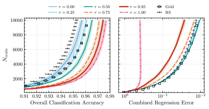
Figure 2: The number of training points needed to achieve a given classification (left panel) and regression (right panel) performance in our synthetic data set test. We define overall classification accuracy using Equation 8 and define regression accuracy as the $90$-th percentile of the distribution of absolute differences. We compare our AL algorithm psy-cris (solid lines) to regularly spaced grids (Grid), and random sampling (RS) while varying $\tau$ and fixing $\beta=2$. In both panels, high performance data sets exist in the bottom right corner, reaching high accuracy or low error with a small training set. Error bars in the combined regression error for Grid and RS are comparable to the size of their respective markers. The psy-cris configuration with $\tau=0.5$ outperforms the regular grid and random sampling in both classification and regression simultaneously.

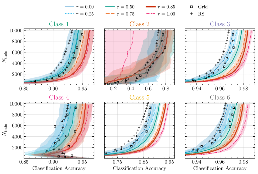
Figure 3: The number of training points needed to achieve a given classification accuracy in our synthetic data test, separated by class. All lines and markers are the same as in Figure 2. We find that all classes exhibit qualitatively similar behavior in performance and improvements from AL. However, features such as the average performance at large $N_{\rm train}$ and the improvements between various AL configurations (different $\tau$), are unique between classes. Class 2 exhibits the largest variance and lowest average performance due to its small size and the fact that it must be discovered by psy-cris in some cases as it may not be present in the starting training set. Class 5 sees the largest gains in performance from AL because of its extended, narrow shape in parameter space (Figure 10) which psy-cris is able to resolve. The errors for random sampling points are similar to the errors shown for the $\tau=0$ line for all classes. The errors for grid points are generally half that width except for Class 2 which has comparable errors throughout.

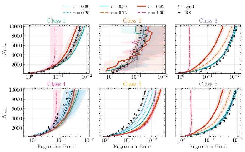
Figure 4: The total number of training points needed to achieve a given regression performance (defined as the $90$-th percentile of the distribution of absolute differences) in our synthetic data set, separated by class. We compare our AL algorithm psy-cris (solid lines) to regularly spaced grids (Grid), and random sampling (RS) while varying $\tau$ and fixing $\beta=2$. We find that for some classes, our best performing configurations of psy-cris slightly outperform Grid and RS. In most cases, the best performing configuration of psy-cris is not $\tau=0$ (which we might expect after seeing the trends in Figure 3), but an intermediate value of $\tau$ which itself is not consistent across classes. Class 5 shows significant gains in regression performance compared to Grid and random sampling, but with the best performing psy-cris configurations focusing more on classification ($\tau>0.5$). However, this behavior is reasonable in cases where classification is challenging, and we see Class 5 has the greatest increases in classification performance when using AL compared to random sampling and regular grids (Figure 3). The errors for grid points are comparable to the size of the markers for all classes. The errors for random sampling points are similarly small except for Class 2 and Class 4 which exhibit errors on the order of the $\tau=0$ line.

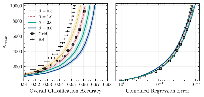
Figure 5: The same as Figure 2 but we fix $\tau=0.5$, the contribution between $\mathcal{C}$ and $\mathcal{R}$ terms, and vary the sharpening parameter $\beta$ as in Equation 2. Increasing $\beta$ results in a higher classification accuracy while not significantly affecting the regression performance. However, at $\beta=3$ we see the regression performance drop slightly. The right choice of $\beta$ will depend on the data set as well as the classification and regression algorithms implemented.

3.2 Synthetic Data Test Summary

Figure 2 shows aggregate performance metrics comparing AL to random sampling and regularly spaced grids at various densities. Since the psy-cris algorithm contains inherent variability from PTMCMC and query point proposals, we show the average of $15$ psy-cris runs where the solid lines are the mean and shaded areas show $68$-th percentile contours. To simulate unique psy-cris runs starting from the same starting grid density, we vary the center of the starting grid randomly by $\pm 1/2$ the bin width in each dimension. This procedure is also used to determine the variance for regular grid configurations at different densities.

For overall classification accuracy (left panel of Figure 2) we find that psy-cris performs significantly better than random sampling (RS) and regularly spaced grids (Grid) when $\tau=1$. As $\tau$ approaches $1$, we find that each subsequent psy-cris configuration achieves higher classification accuracies than the last (on the order of $\sim 0.5\%$) or reaches a target accuracy with significantly smaller number of training points (e.g., for a $\mathrm{CA}{}=96\%$, a factor of two reduction in $N_{\mathrm{train}}$ between Grid and the $\tau=0.75$ model).

For combined regression error (right panel), we see the opposite trend: $\tau$ approaching $0$ gives optimal regression performance. However, the best performing psy-cris configurations do not significantly outperform Grid or RS in regression, and most models converge after $\tau=0.75$. This large scale behavior when changing $\tau$ reflects our design principles when constructing the target distribution in Equation 2.

When considering classification and regression simultaneously with $\tau=0.5$, psy-cris outperforms Grid and RS in classification, and performs similarly to Grid and RS in regression. Conversely, considering only classification ($\tau=1$) or regression ($\tau=0$) alone during AL may lead to significant losses in performance for the neglected category.

We may also consider performance on a class-by-class basis, allowing a more granular perspective on AL performance across the domain. In Figure 3 we show the per-class classification accuracy defined in Equation 9. We find the trends between models at different $\tau$ remain similar to those in overall classification, but some classes achieve larger (Class 5, $\tau=0.5$) or smaller (Class 1, $\tau=0.5$) gains from AL, which is not apparent from Figure 2. Class 5 presents a challenging classification problem because it contains an extended narrow region for $z>0$ (Appendix A), which explains the significant gains from AL compared to other classes. Class 2 is a small class in parameter space that does not necessarily exist in the initial training sets for AL, so it must be discovered by psy-cris in some cases. The process of discovering new classes is stochastic, which explains why Class 2 sees the lowest performance compared to all classes at a given $N_{\mathrm{train}}$. Class 2 is an extreme example of the ML challenges faced when the training set is highly imbalanced. In application of AL, one must carefully evaluate the problem in question to characterize the expected classes and their scale in the domain such that they are represented in the initial training set (Ertekin et al., 2007; Attenberg & Ertekin, 2013).

In Figure 4 we show the per-class regression performance defined as the $90$-th percentile of the distribution of absolute errors. We find that most classes exhibit trends similar to those seen in the overall regression performance. For example, Class 1, Class 3 and Class 6 show the best performing psy-cris runs have $\tau\leq 0.5$. A clear exception is in Class 5, which achieves the highest performance, exceeding Grid and RS, when the contribution factor $\tau>0.5$ weighs classification more heavily in the target distribution. Although this trend may appear to go against our design principles for psy-cris, we expect classification to impact regression performance in challenging cases because our regression algorithms are trained on data separated by class. This difficulty in classification is confirmed by the per-class classification performance in Figure 3 where we see Class 5 benefits the most from AL compared to all other classes. However, considering only classification ($\tau=1$) is not sufficient for reaching the highest regression performance for Class 5 with $\tau=0.85$. In summary, psy-cris performs similarly to regularly spaced grids and random sampling even in the worst cases (e.g., Class 3 and Class 6) and can significantly outperform in others (e.g., Class 5).

We interpret the fact that Grid and RS perform similarly in regression performance to mean that our data can be fit easily with uniformly distributed training data. This is sensible given the regression function (Equation A2) is highly symmetric and smooth, which is not typical for real data.

We also ran models varying the sharpening parameter $\beta$ while fixing $\tau=0.5$, and present aggregate performance results in Figure 5. We find that $\beta$ has a stronger effect on the classification performance than regression performance, and that a larger $\beta$ leads to higher classification accuracy. Although it is difficult to see from Figure 5, there appears to be a difference of $\sim 1000$ points in $N_{\mathrm{train}}$ for a constant regression performance from $\beta=2$ to $\beta=3$. This suggests that $\beta=2$ is close to the optimal value for this data set, and is likely to be a good starting place for problems with similar complexity.

4 Building A MESA Grid

4.1 MESA test setup

The primary goal for our AL algorithm is to construct an optimal set of detailed binary evolution simulations for use in population synthesis codes, such as the MESA simulations being used in POSYDON. An optimal training set provides a target classification and regression accuracy at the lowest computational cost (lowest number of simulations) possible. In this test we demonstrate psy-cris working with POSYDON infrastructure to propose and label MESA simulations (as in Figure 1). We use a python implementation of Message Passing Interface (MPI), combining the software used to run MESA in POSYDON with psy-cris. Implementing distributed computing is critical as it acts as the oracle in the AL loop, automatically running new MESA simulations and post-processing their output.

We model binary systems with a helium (He) main-sequence star and BH companion using MESA’s binary module. We use POSYDON default MESA controls and input parameters, which are described in detail in the POSYDON instrument paper (Fragos et al., 2022) with an additional change. We set the maximum radiative opacity to $0.5~{}\mathrm{cm}^{2}\,\mathrm{g}^{-1}$ for all MESA simulations to alleviate numerical convergence issues as described in Fragos et al. (2022, section 6.1). Our parameter space is the same as the grid of helium-rich stars with companions from Fragos et al. (2022), which covers the initial masses $M_{1}$ of $[0.5M_{\odot},80M_{\odot}]$, $M_{2}$ of $[1M_{\odot},35.88M_{\odot}]$, and the initial orbital period $P_{\mathrm{orb}}$ of $[0.02~{}\mathrm{day},1117.2~{}\mathrm{day}]$.

Part of the POSYDON infrastructure includes parsing MESA outputs to categorize simulations into one of five classes, used to organize data for interpolation (Fragos et al., 2022). The classes are based upon a binary’s characteristic evolution: initial_MT (Roche-lobe overflow at zero-age main-sequence), stable_MT (dynamically stable Roche-lobe overflow mass transfer), unstable_MT (dynamically unstable Roche-lobe overflow mass transfer), no_MT (no Roche-lobe overflow mass transfer), and not_converged (numerical error or exceeded maximum computation time of two days). Numerical convergence issues arise in MESA due to limitations in modeling and often occur in specific regions in parameter space. In the AL phase, we use all five interpolation classes (including the not_converged systems) and only consider regression for the final orbital period for the stable_MT and unstable_MT classes. The not_converged class was included to keep psy-cris from continuously proposing simulations in these problematic regions since any failed run would not add information to the training set, wasting computing resources. We also log-normalize the inputs and outputs from $[-1,1]$ before entering psy-cris and transform the proposal points back into linear space before evolving the system with MESA.

Our parameter space for this test is 3D but can be easily extended into a higher dimensional problem, including covering multiple metallicities to give one example. We compute a high density regular grid with dimensions $41\times 21\times 49$ in $\log_{10}\left(M_{1}/M_{\odot}\right)$, $\log_{10}\left(M_{2}/M_{\odot}\right)$, $\log_{10}\left(P_{\mathrm{orb}}/\mathrm{day}\right)$ respectively totaling $42{,}113$ successful MESA simulations . We choose these dimensions for the regular grid by inspection based on previous tests in the same parameter space. We start psy-cris from a subset of the full density grid by taking every other point in $M_{1}$ and $M_{2}$ and every fourth point in $P_{\mathrm{orb}}$, retaining end points such that the range in each axis matches the full grid. This procedure creates the starting, low density grid with $3{,}003$ MESA simulations. To create the medium-density grid (which we use to compare performance in §4.2) we again use a subset of the full density regular grid, taking every other point in $P_{\mathrm{orb}}$, creating a grid with $21{,}525$ MESA simulations.

During the beginning of AL, the parent MPI process runs one psy-cris iteration which is used to propose the initial parameters for all child processes waiting to run MESA. Once any child process finishes running MESA, the parent process runs psy-cris again with the updated data set and proposes a new point in parameter space to run with MESA (Figure 1). This process is effectively a serial proposal scheme after the initial startup phase, although it depends on the rate at which MESA simulations finish. In our test, psy-cris terminates when a maximum number of proposed points is reached. We stop this test when we could see trends in our performance metrics since this demonstration is computationally expensive. In practice psy-cris is meant to be used for grid sampling until a threshold accuracy in classification, regression, or a combination of the two is achieved. We use a fiducial configuration of psy-cris with parameters taken from the synthetic data tests with $\tau=0.5$ and $\beta=2$.

Unlike with the synthetic data set, the exact outcomes of all MESA simulations in our simulation domain are not known exactly. In order to calculate our standard performance metrics, we create a set by running $10,000$ random uniformly distributed MESA simulations in $\log_{10}(M_{1}/M_{\odot})$, $\log_{10}(M_{2}/M_{\odot})$, and $\log_{10}(P_{\mathrm{orb}}/\mathrm{day})$ .

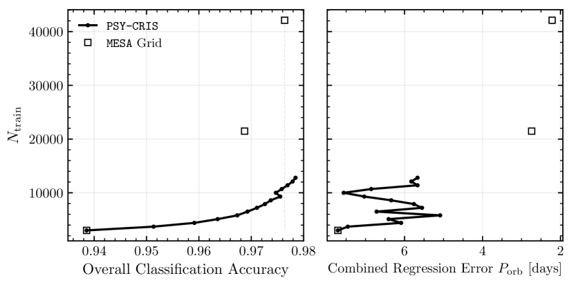
Figure 6: The number of training points needed to achieve a given overall classification accuracy (8) (left panel) and combined regression error (right panel) in our CO–helium-main-sequence MESA test. We use a fiducial configuration of psy-cris with parameters taken from inspecting the synthetic data tests ($\tau=0.5,\beta=2$). The data set consists of 5 classes, two of which we consider regression for the final orbital period ($P_{\mathrm{orb}}$). psy-cris achieves a comparable classification accuracy to the highest density regular grid while using a factor of $\sim 4$ fewer MESA simulations. In regression, psy-cris appears to be approaching lower errors comparable to the medium and full density regular grid, but this trend is not strong. The per-class performance in classification and regression can be found in Figure 7 and Figure 8 respectively.

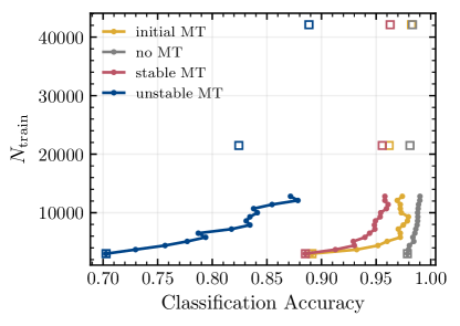
Figure 7: The number of training points necessary to achieve a given per-class classification accuracy (Equation 9) for the MESA test, using psy-cris (solid lines) compared to regularly spaced grids (squares). We use a fifth class (not_converged) when running psy-cris but omit it from performance calculations because it is nonphysical. The stable and unstable mass transfer classes have the lowest performance in the data set. These classes also fall closer to regions in parameter space where many failed runs occur. In all classes we see improvements in classification performance but the most significant gains occur in the unstable mass transfer class.

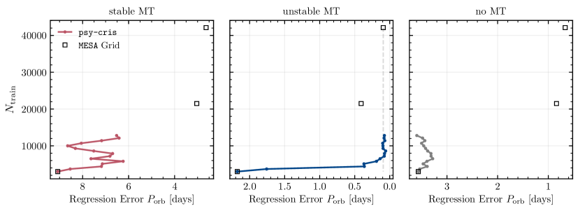
Figure 8: The number of training points necessary to achieve a given regression error per class, defined as the $90$-th percentile of the distribution of absolute differences. The squares in each panel show regression performance for regularly spaced MESA simulations at different densities while psy-cris performance is a solid line. Although the simulations were queried by psy-cris serially, we only show performance calculated every $700$ MESA simulations. The unstable_MT class sees the largest improvements from AL, achieving comparable accuracy to the full density regular grid with a factor of $5.8$ fewer simulations. We do not include regression for the no_MT class during AL, explaining the lack of improvement in regression performance. The stable_MT, unstable_MT, and no_MT classes make up $35\%$ ($22\%$), $9\%$ ($3\%$), and $30\%$ ($60\%$) .

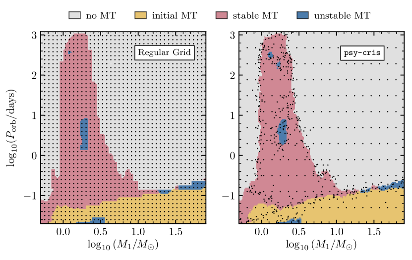
Figure 9: The predicted classification in a slice ($M_{2}\approx 17M_{\odot}$) of our MESA test using a linear classifier trained on the full density regular grid (left panel) and our psy-cris AL data set (right panel). Black dots show the locations of training data within $\pm 1/2$ a logarithmic bin width (defined from the full density regular grid) totalling $2{,}004$ points for the regular grid and $750$ points for psy-cris. The starting grid for psy-cris is a subset of the full density regular grid and contains $3{,}003$ points. psy-cris reproduces the overall structure of the classification space seen in the full density regular grid and resolves finer structure near the class boundaries, while requiring less than half the points. There is a small region of initial_MT simulations labeled as unstable_MT at $\log(P_{\mathrm{orb}}/\mathrm{day})\sim-1.6$ and $\log(M_{1}/M_{\odot})\sim 0.5$ due to an error in the post-processed output.

4.2 MESA test summary

In our MESA test we demonstrate how a fiducial, un-optimized configuration of psy-cris performs in the intended application of creating an AL grid of MESA simulations for use in POSYDON. The process of optimization is highly customized and, hence, not in the scope for this method-demonstration paper.

In Figure 6 we show the overall classification and regression performance between psy-cris and a regular grid for our BH–helium-main-sequence binary simulations. With psy-cris we achieve overall classification accuracy comparable to the densest regular grid with $\sim 4$ times fewer MESA simulations. We also show the combined regression error for the final orbital period $P_{\mathrm{orb}}$ only, because this is the only quantity we use when considering regression during AL. We see that psy-cris reaches errors of $\sim 5~{}\mathrm{day}$ compared to $\sim 2.4~{}\mathrm{day}$ for the medium-density regular grid. While we see that the regression accuracy is decreasing, we do not have enough data to identify a strong trend that can be extrapolated to high $N_{\mathrm{train}}$. We assess that the variability seen in combined (and per-class) regression error is caused by our RBF interpolation, which sets the length scale as the average distance between training data. We do not to optimize for nor fix the length scale since this is only a demonstration of psy-cris. Overall, the performance is consistent with expectations, but to gain a more complete picture, we consider per-class performance for both classification and regression.

In Figure 7 we show the per-class classification accuracy for our MESA test. The stable- and unstable-mass-transfer classes have the lowest accuracies while the no-mass-transfer class starts at nearly $98\%$ accuracy. This is due to the relative size of classes in the parameter space, where small classes generally have lower performance. The unstable-mass-transfer class has the lowest accuracy and sees the largest gains from AL, similar to the challenging case of Class 5 in the synthetic data set. We find that all classes achieve better or comparable per-class classification accuracy with psy-cris at a lower computational cost than the medium density grid. The reduction in number of points required for psy-cris to achieve a comparable per-class accuracy to the medium density regular grid (reduction factor) are given in Table 1. The reduction factor does not translate linearly into CPU-hours saved because not all MESA simulations have the same computational cost.

Table 1: The factor by which we reduce the required number of training points to achieve the same per-class classification accuracy ($\mathrm{PCA}$) and the same F1-score in the MESA test with psy-cris compared to the medium-density regular grid in Figure 7. This is simply $N_{\mathrm{Grid}}/N_{\mathrm{AL}}$ at a fixed $\mathrm{PCA}$ (or F1-score). We calculate F1-score as a secondary metric to compare with our $\mathrm{PCA}$, with both metrics showing similar reduction factors. All psy-cris curves except for unstable_MT for $\mathrm{PCA}$, and initial_MT for F1-score, achieve comparable accuracy to the highest density regular grid by the end of AL to within $<0.5\%$.

	Reduction Factor
Class	$\mathrm{PCA}$	F1-score
initial_MT	4.2	4.2
no_MT	4.9	3.7
stable_MT	2.1	3.3
unstable_MT	2.5	4.2

In Figure 8 we show the absolute error in final orbital period in days for the stable-, unstable-, and no-mass-transfer classes. During AL, we ignore regression for systems undergoing mass transferring at Zero Age Main Sequence (initial_MT) because we expect these systems to result in stellar mergers early in their evolution, in which case their final orbital period is undefined. We also ignore regression for systems that do not have Roche-lobe overflow mass transfer (no_MT) as we assume these systems have comparatively simple evolution, which we are less interested in resolving in this demonstration psy-cris.

The unstable-mass-transfer class sees the greatest improvements in regression accuracy, achieving comparable performance to the full density regular grid with $5.8$ times fewer MESA simulations. This large increase in performance is driven by the fact that the unstable-mass-transfer class is least represented in the data (see Table 2), and AL necessarily populates underrepresented classes (Ertekin et al., 2007). Just as in the synthetic data test, we see that each class has different characteristic performances in regression on the final orbital period; the stable-mass-transfer class has errors on the order of days compared to tenths of days for the unstable-mass-transfer class. The no-mass-transfer class does not achieve any significant improvements in regression, having a nearly constant performance throughout the duration of the AL phase. The stable-mass-transfer class sees some improvements but we do not have enough data to identify strong trends to extrapolate to higher $N_{\mathrm{train}}$.

Finally, Figure 9 shows a slice of our parameter space visualizing the predicted classification after training on the full density regular grid and psy-cris. The starting grid for psy-cris is a subset of the full density regular grid and contains $3{,}003$ points. With AL we resolve classification boundaries and even discover a new region of unstable mass transfer systems at $\log_{10}(P_{\mathrm{orb}}/\mathrm{day})\sim 2.5$, all while requiring $\lesssim 50\%$ the total number of training points of the regular grid. This classification performance has been achieved without optimizing psy-cris for this data set.

Table 2: The percentage of systems in each class in the random test set, the full density regular grid, and the AL data set (AL points combined with the starting sparse grid).

	Data Set Type
Class	Random	Grid	AL
no_MT	60.0	60.3	30.4
stable_MT	20.7	20.6	35.3
initial_MT	10.8	11.1	11.4
not_converged	5.5	4.5	14.0
unstable_MT	3.0	3.5	8.9

5 Discussion

We performed two tests of our AL algorithm psy-cris, on a synthetic data set as well as a real-world application of creating a grid of MESA simulations.

In the synthetic data test, we find that psy-cris can outperform standard methods of sampling in classification and regression by changing the primary free parameters in our algorithm. We also find that only focusing on classification or regression during AL may significantly hinder performance in the neglected category. We then use a fiducial configuration of psy-cris taken from the synthetic data test to construct a dynamic grid of MESA simulations. In this demonstration, we find psy-cris, while not optimized for this data set, is able to achieve comparable overall classification accuracy to the full density regular grid with a factor of $\sim 4$ fewer simulations. We also see significant improvements in per-class regression performance for the unstable-mass-transfer class, achieving comparable performance to the full density regular grid with a factor of $\sim 5.8$ fewer simulations.

The psy-cris algorithm shows promising results for use with MESA grids and is currently being optimized for the POSYDON project. For use in other problems, there are several considerations one should take into account. We use linear interpolation and RBF interpolation from scipy (Jones et al., 2001) to perform classification and regression, respectively. We also use the same interpolation schemes when evaluating all performance metrics for classification and regression. There is a free parameter in the RBF interpolation, the length scale, which by default is set by the average distance between training data. We do not attempt to optimize the length scale in the MESA test which is a naive way to perform regression, and we suspect that this causes poor regression performance in general. In all of our tests we use the same interpolation and classification scheme across all classes, but in practice a more fine-tuned approach is expected to achieve higher accuracies. A more targeted AL regression heuristic may also contribute better performance than shown here.

Concerning AL performance metrics themselves, there are also caveats one should consider. Although we present common performance metrics in this study, there are multiple ways to characterize performance where each metric may highlight specific features while hiding others. For example, our per-class classification definition trivially approaches unity for overconfident classifiers. Imbalanced data sets also present challenges since minority systems may be neglected without affecting cumulative performance metrics significantly (Attenberg & Ertekin, 2013). Therefore, it is important that we explore other performance metrics for AL in POSYDON as we further optimize psy-cris.

It is impossible to guarantee that our AL algorithm, like any AL algorithm, will always outperform standard sampling (e.g., Dasgupta, 2005; Settles & Craven, 2008; Yang & Loog, 2018). Our algorithm works for our use case, and it is worth consideration in computationally-challenging problems involving high-dimensional data showing complicated structure and behavior.

However, we have shown psy-cris already achieves promising performance in three dimensions, matching the MESA grids being used in POSYDON v1. In our demonstration, we are already seeing up to factors of $4$ reduction in the number of simulations to achieve a comparable accuracy with AL to high density rectilinear grids.

6 Conclusions

Our aim is to efficiently construct data sets of binary evolution simulations with reliable interpolation accuracy to be used in the population synthesis codes such as POSYDON. Regular grids of binary evolution simulations can require prohibitively large computational resources to construct due to the cost per simulation combined with the parameter space we must cover to adequately characterizes binary stellar evolution. We propose AL as a solution for constructing high performance training sets of binary evolution simulations, at a reduced cost compared to standard methods. We demonstrate our new AL algorithm psy-cris tested on a synthetic data set and a realistic data set of binary evolution simulations with MESA.

In our initial synthetic data set test, we find that psy-cris can be optimized to outperform standard methods of sampling by varying the free parameters in our model. We find that focusing just on classification or regression alone may lead to significant losses in performance in the neglected category. Therefore it is essential to consider both to obtain well-adapted results. When considering per-class performance, we see major gains from AL in both classification and regression for classes which present challenging classification problems, characterized by extended and narrow shapes in parameter space (Class 5). We also see low performance occurs for minority classes in imbalanced data sets, as well as a class’s presence (or absence) in the initial training set (Class 2). psy-cris does indirectly address data imbalances by weighting each class equally (Table 2) but a more active approach may achieve better results. Different classes will have different characteristic performances based off their size and shape in parameter space, and may also benefit the most from AL in challenging cases.

We also demonstrate psy-cris working with POSYDON infrastructure to evolve binary systems consisting of a CO and helium-main-sequence star with MESA. We use an unoptimized configuration of psy-cris, determined from the synthetic data set tests, and find that psy-cris outperforms the highest density regular grid in overall classification using a quarter the total number of training points. In regression we see psy-cris is reducing the regression error but not yet to the level of the medium density regular grid.

Creating the oracle in our AL loop was critically important for running simulations with MESA. Not only does the oracle label simulations automatically, but it ensures that we encounter fewer numerical difficulties that commonly arise in MESA. In our MESA test, $14\%$ of our AL data set consists of failed simulations, which do not terminate normally due to numerical convergence issues (Table 2). Minimizing numerical convergence issues in our binary simulations with MESA will only further improve the AL results in POSYDON.

Since each POSYDON data set will exhibit unique classification and regression challenges, psy-cris may benefit from further optimization specific to each binary evolution grid. For instance, one could consider different AL metrics such as the classification entropy (e.g., Gal et al., 2017; Cai et al., 2017; Yang & Loog, 2018). Currently, psy-cris has been designed to consider initial–final quantities alone, but our MESA simulations have time series evolution in between these end points. Therefore, in the future we are interested in seeing how psy-cris will respond to the complexity of their time series evolution as a metric for simulation proposals. Furthermore, we could factor in the varying computing cost of different simulations to pick the most informative points in parameter space per unit CPU time (Tomanek & Hahn, 2010; Kumar & Gupta, 2020).

Although we have designed it to optimize our generation of binary evolution grids as part of the POSYDON code, psy-cris is a general algorithm that can be applied to data sets with classification and regression outputs. To be applied directly in another similar problem, one must construct the oracle (which will label and run new simulations) to completely automate the AL loop. The psy-cris AL approach will work best for optimizing large grids of simulations where the number of simulated points is too large to optimize manually, and brute-force oversampling is too computationally expensive. Examples are numerical relativity simulations for building gravitational-wave approximants (Varma et al., 2019; Healy & Lousto, 2022), or large grids of kilonova models (Ristic et al., 2022). The psy-cris code is open source, and exists as a module in POSYDON which will be available in the next release of POSYDON.

Appendix A Constructing the Synthetic Data Set

In Section 3 we test our AL algorithm psy-cris in a 3D synthetic data set by comparing classification and regression performance of training sets built with psy-cris to regularly spaced grids and random sampling. We chose a synthetic data set for its cheap computational cost for labeling queries and its deterministic output. The fiducial range of the synthetic data set is $(-1,1)$ for all dimensions. The data set contains six unique classes and one regression function, continuous across all classes.

To construct the classification space, we use analytic functions and arbitrary constants (split values) to define binary classification boundaries. With the first function, two classes are created, and each subsequent function adds one more unique class to the parameter space. The five functions that define our classification space are given by

$${\psi}_{1}(x,y,z) =\displaystyle\left(\frac{x+1}{1.2}\right)^{2}+\left(\frac{y-1}{2}\right)^{2}+\left(\frac{z}{0.8}\right)^{2}-1,$$ (A1a)

$${\psi}_{2}(x,y,z) =(1-x)^{2}+3(y-x^{2})^{2}+|z|(x-z)^{2},$$ (A1b)

$${\psi}_{3}(x,y,z) =\sin(x-0.25)+yz,$$ (A1c)

$${\psi}_{4}(x,y,z) =|x^{3}-y^{3}|\exp[-z],$$ (A1d)

$${\psi}_{5}(x,y,z) =\left(\frac{x-0.5}{0.6}\right)^{2}+\left(\frac{y-0.5}{0.2}\right)^{2}+\left(\frac{z-0.85}{0.3}\right)^{2}-0.2^{2},$$ (A1e)

where $x$, $y$, and $z$ are inputs in Cartesian coordinates. We combine each function and their associated split values into inequalities such that any input will be mapped to True or False for each function. We provide a pseudo-code function for the classification of an arbitrary point in our domain,

    def classification(x,y,z):
        if psi_5(x,y,z) < 0.3:
            return "Class 2"
        elif psi_4(x,y,z) > 1.8 and z < 0:
            return "Class 4"
        elif psi_1(x,y,z) > 1 and psi_2(x,y,z) > 2.5:
            return "Class 1"
        elif psi_2(x,y,z) > 2.5:
            return "Class 6"
        elif psi_3(x,y,z) > -0.5:
            return "Class 3"
        else:
            return "Class 5"

where methods psi_1 through psi_5 correspond to the functions in Equation A1. Finally, we have the regression function $\psi_{6}$ which is a 3D sinusoid, spherically symmetric about the origin. We chose to use the same function for all classes even though psy-cris treats each class’ regression output separately.

$$\psi_{6}(x,y,z)=\sin\left(8\pi\sqrt{x^{2}+y^{2}+z^{2}}/3\right).$$ (A2)

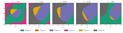
Figure 10: The true classification space for the synthetic data set, constructed with the analytic functions provided in Equation A1. The regression output from Equation A2 is defined in the same range, and together they make up the synthetic data set.

References

- Andrews et al. (2018) Andrews, J. J., Zezas, A., & Fragos, T. 2018, ApJS, 237, 1, doi: 10.3847/1538-4365/aaca30
- Attenberg & Ertekin (2013) Attenberg, J., & Ertekin, S. 2013, Class Imbalance and Active Learning (John Wiley & Sons, Ltd), 101–149, doi: 10.1002/9781118646106.ch6
- Barrett et al. (2018) Barrett, J. W., Gaebel, S. M., Neijssel, C. J., et al. 2018, MNRAS, 477, 4685, doi: 10.1093/mnras/sty908
- Belczynski et al. (2002) Belczynski, K., Kalogera, V., & Bulik, T. 2002, ApJ, 572, 407, doi: 10.1086/340304
- Belczynski et al. (2008) Belczynski, K., Kalogera, V., Rasio, F. A., et al. 2008, ApJS, 174, 223, doi: 10.1086/521026
- Bollig et al. (2021) Bollig, R., Yadav, N., Kresse, D., et al. 2021, ApJ, 915, 28, doi: 10.3847/1538-4357/abf82e
- Breivik et al. (2020) Breivik, K., Coughlin, S., Zevin, M., et al. 2020, ApJ, 898, 71, doi: 10.3847/1538-4357/ab9d85
- Broekgaarden et al. (2019) Broekgaarden, F. S., Justham, S., de Mink, S. E., et al. 2019, MNRAS, 490, 5228, doi: 10.1093/mnras/stz2558
- Cai et al. (2017) Cai, W., Zhang, M., & Zhang, Y. 2017, IEEE Transactions on Neural Networks and Learning Systems, 28, 1668, doi: 10.1109/TNNLS.2016.2542184
- Caron et al. (2019) Caron, S., Heskes, T., Otten, S., & Stienen, B. 2019, European Physical Journal C, 79, 944, doi: 10.1140/epjc/s10052-019-7437-5
- Choi et al. (2016) Choi, J., Dotter, A., Conroy, C., et al. 2016, ApJ, 823, 102, doi: 10.3847/0004-637X/823/2/102
- Daningburg & O’Shaughnessy (2022) Daningburg, K., & O’Shaughnessy, R. 2022, arXiv e-prints, arXiv:2205.07987. https://arxiv.org/abs/2205.07987
- Dasgupta (2005) Dasgupta, S. 2005, in Advances in Neural Information Processing Systems, ed. L. Saul, Y. Weiss, & L. Bottou, Vol. 17 (MIT Press)
- de Mink et al. (2007) de Mink, S. E., Pols, O. R., & Hilditch, R. W. 2007, A&A, 467, 1181, doi: 10.1051/0004-6361:20067007
- Demir et al. (2011) Demir, B., Persello, C., & Bruzzone, L. 2011, IEEE Transactions on Geoscience and Remote Sensing, 49, 1014, doi: 10.1109/TGRS.2010.2072929
- Doctor et al. (2017) Doctor, Z., Farr, B., Holz, D. E., & Pürrer, M. 2017, Phys. Rev. D, 96, 123011, doi: 10.1103/PhysRevD.96.123011
- Earl & Deem (2005) Earl, D. J., & Deem, M. W. 2005, Physical Chemistry Chemical Physics (Incorporating Faraday Transactions), 7, 3910, doi: 10.1039/B509983H
- Eldridge et al. (2017) Eldridge, J. J., Stanway, E. R., Xiao, L., et al. 2017, PASA, 34, e058, doi: 10.1017/pasa.2017.51
- Ertekin et al. (2007) Ertekin, S., Huang, J., Bottou, L., & Giles, L. 2007, in Proceedings of the Sixteenth ACM Conference on Conference on Information and Knowledge Management, CIKM ’07 (New York, NY, USA: Association for Computing Machinery), 127–136, doi: 10.1145/1321440.1321461
- Farmer et al. (2015) Farmer, R., Fields, C. E., & Timmes, F. X. 2015, ApJ, 807, 184, doi: 10.1088/0004-637X/807/2/184
- Fragos et al. (2015) Fragos, T., Linden, T., Kalogera, V., & Sklias, P. 2015, ApJ, 802, L5, doi: 10.1088/2041-8205/802/1/L5
- Fragos et al. (2022) Fragos, T., Andrews, J. J., Bavera, S. S., et al. 2022, arXiv e-prints, arXiv:2202.05892. https://arxiv.org/abs/2202.05892
- Gal et al. (2017) Gal, Y., Islam, R., & Ghahramani, Z. 2017, arXiv e-prints, arXiv:1703.02910. https://arxiv.org/abs/1703.02910
- Gallegos-Garcia et al. (2021) Gallegos-Garcia, M., Berry, C. P. L., Marchant, P., & Kalogera, V. 2021, ApJ, 922, 110, doi: 10.3847/1538-4357/ac2610
- García et al. (2021) García, F., Simaz Bunzel, A., Chaty, S., Porter, E., & Chassande-Mottin, E. 2021, A&A, 649, A114, doi: 10.1051/0004-6361/202038357
- Giacobbo et al. (2018) Giacobbo, N., Mapelli, M., & Spera, M. 2018, MNRAS, 474, 2959, doi: 10.1093/mnras/stx2933
- Han et al. (2020) Han, Z.-W., Ge, H.-W., Chen, X.-F., & Chen, H.-L. 2020, Research in Astronomy and Astrophysics, 20, 161, doi: 10.1088/1674-4527/20/10/161
- Hastings (1970) Hastings, W. K. 1970, Biometrika, 57, 97, doi: 10.1093/biomet/57.1.97
- Healy & Lousto (2022) Healy, J., & Lousto, C. O. 2022, arXiv e-prints, arXiv:2202.00018. https://arxiv.org/abs/2202.00018
- Hoi et al. (2006) Hoi, S. C. H., Jin, R., Zhu, J., & Lyu, M. R. 2006, in Proceedings of the 23rd International Conference on Machine Learning, ICML ’06 (New York, NY, USA: Association for Computing Machinery), 417–424, doi: 10.1145/1143844.1143897
- Hunter (2007) Hunter, J. D. 2007, Computing in Science Engineering, 9, 90, doi: 10.1109/MCSE.2007.55
- Hurley et al. (2000) Hurley, J. R., Pols, O. R., & Tout, C. A. 2000, MNRAS, 315, 543, doi: 10.1046/j.1365-8711.2000.03426.x
- Hurley et al. (2002) Hurley, J. R., Tout, C. A., & Pols, O. R. 2002, MNRAS, 329, 897, doi: 10.1046/j.1365-8711.2002.05038.x
- Ishida et al. (2019) Ishida, E. E. O., Beck, R., González-Gaitán, S., et al. 2019, MNRAS, 483, 2, doi: 10.1093/mnras/sty3015
- Izzard et al. (2006) Izzard, R. G., Dray, L. M., Karakas, A. I., Lugaro, M., & Tout, C. A. 2006, A&A, 460, 565, doi: 10.1051/0004-6361:20066129
- Izzard et al. (2009) Izzard, R. G., Glebbeek, E., Stancliffe, R. J., & Pols, O. R. 2009, A&A, 508, 1359, doi: 10.1051/0004-6361/200912827
- Izzard et al. (2004) Izzard, R. G., Tout, C. A., Karakas, A. I., & Pols, O. R. 2004, MNRAS, 350, 407, doi: 10.1111/j.1365-2966.2004.07446.x
- Jones et al. (2001) Jones, E., Oliphant, T., Peterson, P., et al. 2001, SciPy: Open source scientific tools for Python. http://www.scipy.org/
- Joshi et al. (2009) Joshi, A. J., Porikli, F., & Papanikolopoulos, N. 2009, in 2009 IEEE Conference on Computer Vision and Pattern Recognition, 2372–2379, doi: 10.1109/CVPR.2009.5206627
- Kennamer et al. (2020) Kennamer, N., Ishida, E. E. O., Gonzalez-Gaitan, S., et al. 2020, arXiv e-prints, arXiv:2010.05941. https://arxiv.org/abs/2010.05941
- King et al. (2004) King, R. D., Whelan, K. E., Jones, F. M., et al. 2004, Nature, 427, 247, doi: 10.1038/nature02236
- Kruckow et al. (2018) Kruckow, M. U., Tauris, T. M., Langer, N., Kramer, M., & Izzard, R. G. 2018, MNRAS, 481, 1908, doi: 10.1093/mnras/sty2190
- Kumar & Gupta (2020) Kumar, P., & Gupta, A. 2020, Journal of Computer Science and Technology, 35, 913, doi: 10.1007/s11390-020-9487-4
- Lewis & Gale (1994) Lewis, D. D., & Gale, W. A. 1994, arXiv e-prints, cmp. https://arxiv.org/abs/cmp-lg/9407020
- Lipunov et al. (1996) Lipunov, V. M., Postnov, K. A., & Prokhorov, M. E. 1996, The scenario machine: Binary star population synthesis
- Lipunov et al. (2009) Lipunov, V. M., Postnov, K. A., Prokhorov, M. E., & Bogomazov, A. I. 2009, Astronomy Reports, 53, 915, doi: 10.1134/S1063772909100047
- Marchant et al. (2021) Marchant, P., Pappas, K. M. W., Gallegos-Garcia, M., et al. 2021, A&A, 650, A107, doi: 10.1051/0004-6361/202039992
- McKinney et al. (2010) McKinney, W., et al. 2010, in Proceedings of the 9th Python in Science Conference, Vol. 445, Austin, TX, 51–56
- Mehrjou et al. (2018) Mehrjou, A., Khodabandeh, M., & Mori, G. 2018, arXiv e-prints, arXiv:1805.08916. https://arxiv.org/abs/1805.08916
- Metropolis et al. (1953) Metropolis, N., Rosenbluth, A. W., Rosenbluth, M. N., Teller, A. H., & Teller, E. 1953, J. Chem. Phys., 21, 1087, doi: 10.1063/1.1699114
- Misra et al. (2020) Misra, D., Fragos, T., Tauris, T. M., Zapartas, E., & Aguilera-Dena, D. R. 2020, A&A, 642, A174, doi: 10.1051/0004-6361/202038070
- Müller et al. (2017) Müller, B., Melson, T., Heger, A., & Janka, H.-T. 2017, MNRAS, 472, 491, doi: 10.1093/mnras/stx1962
- Nelson & Eggleton (2001) Nelson, C. A., & Eggleton, P. P. 2001, ApJ, 552, 664, doi: 10.1086/320560
- Nelson et al. (2018) Nelson, D., Pillepich, A., Springel, V., et al. 2018, MNRAS, 475, 624, doi: 10.1093/mnras/stx3040
- Paxton et al. (2011) Paxton, B., Bildsten, L., Dotter, A., et al. 2011, ApJS, 192, 3, doi: 10.1088/0067-0049/192/1/3
- Paxton et al. (2013) Paxton, B., Cantiello, M., Arras, P., et al. 2013, ApJS, 208, 4, doi: 10.1088/0067-0049/208/1/4
- Paxton et al. (2015) Paxton, B., Marchant, P., Schwab, J., et al. 2015, ApJS, 220, 15, doi: 10.1088/0067-0049/220/1/15
- Paxton et al. (2018) Paxton, B., Schwab, J., Bauer, E. B., et al. 2018, ApJS, 234, 34, doi: 10.3847/1538-4365/aaa5a8
- Paxton et al. (2019) Paxton, B., Smolec, R., Schwab, J., et al. 2019, ApJS, 243, 10, doi: 10.3847/1538-4365/ab2241
- Pedregosa et al. (2011) Pedregosa, F., Varoquaux, G., Gramfort, A., et al. 2011, Journal of Machine Learning Research, 12, 2825
- Portegies Zwart (2020) Portegies Zwart, S. 2020, Nature Astronomy, 4, 819, doi: 10.1038/s41550-020-1208-y
- Portegies Zwart & Verbunt (1996) Portegies Zwart, S. F., & Verbunt, F. 1996, A&A, 309, 179
- Rasmussen & Williams (2006) Rasmussen, C. E., & Williams, C. K. I. 2006, Gaussian Processes for Machine Learning
- Richards et al. (2012) Richards, J. W., Starr, D. L., Brink, H., et al. 2012, ApJ, 744, 192, doi: 10.1088/0004-637X/744/2/192
- Riley et al. (2022) Riley, J., Agrawal, P., Barrett, J., et al. 2022, The Journal of Open Source Software, 7, 3838, doi: 10.21105/joss.03838
- Ristic et al. (2022) Ristic, M., Champion, E., O’Shaughnessy, R., et al. 2022, Physical Review Research, 4, 013046, doi: 10.1103/PhysRevResearch.4.013046
- Román-Garza et al. (2021) Román-Garza, J., Bavera, S. S., Fragos, T., et al. 2021, ApJ, 912, L23, doi: 10.3847/2041-8213/abf42c
- Schohn & Cohn (2000) Schohn, G., & Cohn, D. 2000, in Proceedings of the Seventeenth International Conference on Machine Learning, ICML ’00 (San Francisco, CA, USA: Morgan Kaufmann Publishers Inc.), 839–846
- Sener & Savarese (2017) Sener, O., & Savarese, S. 2017, arXiv e-prints, arXiv:1708.00489. https://arxiv.org/abs/1708.00489
- Settles (2009) Settles, B. 2009, Active Learning Literature Survey, Computer Sciences Technical Report 1648, University of Wisconsin–Madison
- Settles & Craven (2008) Settles, B., & Craven, M. 2008, in Proceedings of the Conference on Empirical Methods in Natural Language Processing, EMNLP ’08 (USA: Association for Computational Linguistics), 1070–1079
- Solorio et al. (2005) Solorio, T., Fuentes, O., Terlevich, R., & Terlevich, E. 2005, MNRAS, 363, 543, doi: 10.1111/j.1365-2966.2005.09456.x
- Spera et al. (2015) Spera, M., Mapelli, M., & Bressan, A. 2015, MNRAS, 451, 4086, doi: 10.1093/mnras/stv1161
- Spera et al. (2019) Spera, M., Mapelli, M., Giacobbo, N., et al. 2019, MNRAS, 485, 889, doi: 10.1093/mnras/stz359
- Springel (2010) Springel, V. 2010, MNRAS, 401, 791, doi: 10.1111/j.1365-2966.2009.15715.x
- Stevenson et al. (2017) Stevenson, S., Vigna-Gómez, A., Mandel, I., et al. 2017, Nature Communications, 8, 14906, doi: 10.1038/ncomms14906
- Swendsen & Wang (1986) Swendsen, R. H., & Wang, J.-S. 1986, Phys. Rev. Lett., 57, 2607, doi: 10.1103/PhysRevLett.57.2607
- Tomanek & Hahn (2010) Tomanek, K., & Hahn, U. 2010, in Proceedings of the 23rd International Conference on Computational Linguistics: Posters, COLING ’10 (USA: Association for Computational Linguistics), 1247–1255
- Toonen et al. (2012) Toonen, S., Nelemans, G., & Portegies Zwart, S. 2012, A&A, 546, A70, doi: 10.1051/0004-6361/201218966
- van der Walt et al. (2011) van der Walt, S., Colbert, S. C., & Varoquaux, G. 2011, Computing in Science Engineering, 13, 22, doi: 10.1109/MCSE.2011.37
- Varma et al. (2019) Varma, V., Field, S. E., Scheel, M. A., et al. 2019, Phys. Rev. Research., 1, 033015, doi: 10.1103/PhysRevResearch.1.033015
- Vartanyan et al. (2019) Vartanyan, D., Burrows, A., Radice, D., Skinner, M. A., & Dolence, J. 2019, MNRAS, 482, 351, doi: 10.1093/mnras/sty2585
- Wang et al. (2021) Wang, Y., Liu, X., Zhu, W., Tang, L., & Lin, W. 2021, ApJ, 906, 129, doi: 10.3847/1538-4357/abcc66
- Wang et al. (2017) Wang, Z., Du, B., Zhang, L., Zhang, L., & Jia, X. 2017, IEEE Transactions on Geoscience and Remote Sensing, 55, 3071, doi: 10.1109/TGRS.2017.2650938
- Wellstein & Langer (1999) Wellstein, S., & Langer, N. 1999, A&A, 350, 148. https://arxiv.org/abs/astro-ph/9904256
- Yang & Loog (2018) Yang, Y., & Loog, M. 2018, Pattern Recognition, 83, 401, doi: https://doi.org/10.1016/j.patcog.2018.06.004