First-principles Landau-like potential for BiFeO₃ and related materials

Abstract

In this work we introduce the simplest, lowest-order Landau-like potential for BiFeO₃ and La-doped BiFeO₃ as an expansion around the paraelectric cubic phase in powers of polarization, FeO₆ octahedral rotations and strains. We present an analytical approach for computing the model parameters from density functional theory. We illustrate our approach by computing the potentials for BiFeO₃ and La_0.25Bi_0.75FeO₃ and show that, overall, we are able to capture the first-principles results accurately. The computed models allow us to identify and explain the main interactions controlling the relative stability of the competing low-energy phases of these compounds.

I Introduction

Magnetoelectric multiferroics, materials that simultaneously show magnetic and electric orders, are of significant interest, since the coexistence and coupling of these orders hold great potential for development of multifunctional devices Spaldin and Fiebig (2005); Eerenstein et al. (2006). BiFeO₃ is among the most exciting and extensively studied representatives of this family because it displays both orders at room temperature Catalan and Scott (2009).

Ferroelectricity appears in BiFeO₃ at $T_{C}\sim 1100$ K Moreau et al. (1971); Smith et al. (1968). Below $T_{C}$, it has a rhombohedrally distorted perovskite structure (space group $R3c$, #161) Michel et al. (1969); Kubel and Schmid (1990), which differs from the perfect cubic phase by the presence of two distortions: (i) polar displacements of Bi³⁺ and Fe³⁺ cations with respect to O^2- anions (Bi³⁺ dominates due to its stereochemically active $6s$ lone pairs Seshadri and Hill (2001)) giving rise to a spontaneous polarization $\mathbf{P}$ of up to 100 $\mu$C/cm² along a pseudocubic $\langle 111\rangle$ direction Lebeugle et al. (2007); Wang et al. (2003); and (ii) antiphase rotations $\mathbf{R}$ of the FeO₆ octahedra about the same pseudocubic $\langle 111\rangle$ direction as the polarization ($a^{-}a^{-}a^{-}$ in Glazer’s notation Glazer (1972)) Ederer and Spaldin (2005); Diéguez et al. (2011). (In the following, all directions are in the pseudocubic setting.)

Below $T_{N}\sim 640$ K, BiFeO₃ also shows G-type antiferromagnetic (G-AFM) order with the nearest-neighboring Fe spins antialigned Bhide and Multani (1965); Moreau et al. (1971). The canting of the Fe spins driven by Dzyaloshinskii-Moriya (DM) interaction Dzyaloshinsky (1958); Moriya (1960) can give rise to a weak magnetization in this material. The DM interaction relies on the symmetry breaking caused by the FeO₆ octahedral tilts of BiFeO₃ Ederer and Spaldin (2005); indeed, the phase of the octahedral rotations defines the sign of the DM vector and, in turn, that of the weak magnetization. In bulk BiFeO₃ an incommensurate cycloidal spiral is superimposed on the G-AFM order, yielding a zero net magnetization Sosnowska et al. (1982). This cycloid, however, can be suppressed by doping in bulk systems Sosnowska et al. (2002) and by epitaxial constraints in BiFeO₃ films Bai et al. (2005); Béa et al. (2007); Sando et al. (2013); Heron et al. (2014). Therefore, ferroelectricity can coexist with weak ferromagnetism in BiFeO₃ at ambient conditions.

Additionally, a 180^∘ deterministic switching of the DM vector and weak magnetization by an electric field has been reported from a combined experimental and theoretical study of BiFeO₃ films grown on DyScO₃ substrates Heron et al. (2014). It is proposed that the magnetoelectric switching is the result of a peculiar polarization reversal that is found to occur in two steps, a 109^∘ rotation followed by a 71^∘ rotation (or vice versa); further, the FeO₆ octahedral tilts are believed to reverse together with the polarization, resulting in the observed reversal of the weak magnetic moment. Note that octahedral tilts will typically not follow polarization in a single-step 180^∘ reversal and, therefore, a two-step switching path is crucial for controlling the weak magnetization in BiFeO₃ by an electric field. These observations make BiFeO₃ a promising candidate for applications in magnetoelectric memory elements. However, to be technologically relevant, switching characteristics have to be optimized such that coercive voltages are below 100 mV and switching times fall in the range of 10-1000 ps Manipatruni et al. (2018); Prasad et al. (2020). Hence, the current challenge is to optimize the ferroelectric switching in BiFeO₃ while retaining the two-step path and magnetoelectric control.

One of the efficient strategies for optimizing polarization switching in BiFeO₃ is doping by La. Indeed, since polarization in this compound largely originates from the $6s$ lone pairs of the Bi³⁺ cations, their substitution by isovalent, lone-pair-free cations leads to a reduction of the polar distortion Catalan and Scott (2009); Chu et al. (2008); González-Vázquez et al. (2012). For example, it has been experimentally demonstrated that 15-20% La-doped BiFeO₃ films show a polarization which is up to 60% smaller than that of pure BiFeO₃ films Prasad et al. (2020); Zhang et al. (2019). Further, first-principles calculations have predicted that subsitution of Bi by La cations reduces the energy barrier between polar states by up to 50% for 25% doping. This, in turn, leads to a reduction of coercive voltages (down to 0.8 V for a 100 nm film), enabling low-power switching Prasad et al. (2020). Additionally, a significant reduction of switching times has been demonstrated for La_0.15Bi_0.75FeO₃ films compared to pure BiFeO₃ in a wide range of applied electric fields Parsonnet et al. (2020). Nevertheless, further improvement requires understanding the origin of the two-step polarization switching in BiFeO₃ and related materials, as well as search for other strategies for manipulating the switching energy landscape. For that purpose, dynamical simulations of polarization switching based on phenomenological models of the free energy can be very helpful.

Landau free-energy potentials Landau (1937a, b); Devonshire (1949, 1951), together with the Landau-Khalatnikov time-evolution equation Umantsev (2012), offer a practical scheme to investigate switching in ferroelectrics. In this approach, one expands the energy of the compound around the reference paraelectric phase in powers of the relevant order parameters, keeping only terms compatible with the crystal symmetry K. M. Rabe (2007). It is important to note that the reliability of such simulations depends on the choice of the free energy expansion’s coefficients, which can be obtained either by fitting to experimental data or from first-principles calculations K. M. Rabe (2007). In compounds as complex as BiFeO₃, which feature multiple primary order parameters, deriving a suitable Landau potential from experimental information is all but impossible; hence, there is a clear need for the development of first-principles approaches.

In this work we introduce the simplest, lowest-order Landau-like potential able to reproduce the energies and structures of the low-energy polymorphs of BiFeO₃ and related materials. We present an analytical approach to compute the model parameters from density functional theory (DFT) and apply it to BiFeO₃ and La_0.25Bi_0.75FeO₃. We demonstrate the overall accuracy of the obtained potentials, and discuss an effective way to treat intermediate compositions. Finally, we discuss the physics captured by the model, namely, the interaction between polarization and FeO₆ octahedral tilts, how it affects the energetics of different BiFeO₃ polymorphs, as well as the effects of La doping.

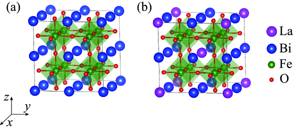
Figure 1: Sketch of the 40-atom supercell used in our simulations of (a) BiFeO₃ and (b) La_0.25Bi_0.75FeO₃.

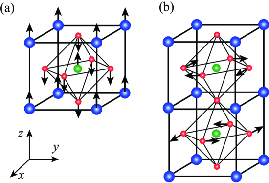
Figure 2: Ionic displacement patterns corresponding to (a) a polar distortion mode along the [001] pseudocubic direction and (b) FeO₆ octahedral rotations about the same axis. Arrows indicate the directions of the ionic displacements and do not reflect their relative amplitudes. Blue, green and red circles indicate Bi, Fe and O ions, respectively.

II Computational details

All calculations are performed using the DFT Hohenberg and Kohn (1964); Kohn and Sham (1965) implementation in the Vienna Ab initio Simulation package (VASP) Kresse and Furthmüller (1996). For the exchange-correlation potential, we use the generalized gradient approximation optimized for solids Perdew et al. (2008), with a Hubbard $U$ correction (within Dudarev’s scheme Dudarev et al. (1998) and $U=4$ eV) for a better treatment of iron’s 3$d$ electrons. We treat the interaction between core and valence electrons by the projector-augmented plane wave method Blöchl (1994); Kresse and Furthmüller (1996), solving explicitly for 15 electrons of Bi ($5d^{10}6s^{2}6p^{3}$), 9 of La ($5p^{6}6s^{2}5d^{1}$), 14 of Fe ($3p^{6}3d^{7}4s^{1}$), and 6 of O ($2s^{2}2p^{4}$). We use a plane-wave basis set with a cutoff energy of 500 eV. We use a $3\times 3\times 3$ $\Gamma$-centered Monkhorst-Pack $k$-point grid for reciprocal space integrals in the Brillouin zone corresponding to a 40-atom cell that is a 2$\times$2$\times$2 multiple of the 5-atom perovskite unit (see Fig. 1(a)). We ensure that these choices provide a good level of convergence for the quantities of interest. All simulations are performed with the G-type antiferromagnetic order of Fe magnetic moments imposed. In the lattice optimizations, the structures are considered to be relaxed when the forces acting on the atoms are below 0.01 eV/Å. We calculate elastic constants by finite differences using the strain-stress relationship Le Page and Saxe (2002).

III Formalism

III.1 Landau-like potential

In this section we introduce the potential for BiFeO₃ and La-doped BiFeO₃ as an expansion around the reference paraelectric cubic phase in powers of the following order parameters: (i) the three-dimensional electric polarization $\mathbf{P}=(P_{x},P_{y},P_{z})$; (ii) the antiphase rotations of FeO₆ octahedra $\mathbf{R}=(R_{x},R_{y},R_{z})$; (iii) the strain $\bm{\eta}=(\eta_{xx},\eta_{yy},\eta_{zz},\eta_{yz},\eta_{xz},\eta_{xy})$, where $\eta_{xx}=\epsilon_{xx}$, $\eta_{yy}=\epsilon_{yy}$, $\eta_{zz}=\epsilon_{zz}$, $\eta_{yz}=2\epsilon_{yz}$, $\eta_{xz}=2\epsilon_{xz}$ and $\eta_{xy}=2\epsilon_{xy}$, and $\epsilon_{ij}$ are the components of the homogeneous strain tensor. The resulting expression for the potential (per perovskite unit cell) is written as follows:

$$F(P,R,\eta)= F_{0}+F(P)+F(R)+F(\eta)+$$ (1)

$$F(P,R)+F(P,\eta)+F(R,\eta).$$

Here, $F_{0}$ is the free energy of the reference cubic phase. $F(P)$, $F(R)$ and $F(\eta)$ are the energy contributions solely due to polarization, FeO₆ octahedral rotations and strain, respectively, which we write as follows:

$$F(P)= A_{P}(P_{x}^{2}+P_{y}^{2}+P_{z}^{2})+B_{P}(P_{x}^{2}+P_{y}^{2}+P_{z}^{2})^{2}+$$ (2)

$$C_{P}(P_{x}^{2}P_{y}^{2}+P_{y}^{2}P_{z}^{2}+P_{z}^{2}P_{x}^{2});$$

$$F(R)= A_{R}(R_{x}^{2}+R_{y}^{2}+R_{z}^{2})+B_{R}(R_{x}^{2}+R_{y}^{2}+R_{z}^{2})^{2}+$$ (3)

$$C_{R}(R_{x}^{2}R_{y}^{2}+R_{y}^{2}R_{z}^{2}+R_{z}^{2}R_{x}^{2});$$

$$F(\eta)= \frac{1}{2}C_{11}(\eta_{xx}^{2}+\eta_{yy}^{2}+\eta_{zz}^{2})+C_{12}(\eta_{xx}\eta_{yy}+$$ (4)

$$\eta_{yy}\eta_{zz}+\eta_{zz}\eta_{xx})+\frac{1}{2}C_{44}(\eta_{yz}^{2}+\eta_{xz}^{2}+\eta_{xy}^{2}).$$

We truncate the expansion in $\mathbf{P}$ and $\mathbf{R}$ at the fourth order, which is the minimum required to model structural instabilities. In turn, we only consider harmonic terms for the strains.

Then, $F(P,R)$, $F(P,\eta)$ and $F(R,\eta)$ are the coupling terms, which we write as:

$$F( P,R)=B_{PR}(P_{x}^{2}+P_{y}^{2}+P_{z}^{2})(R_{x}^{2}+R_{y}^{2}+R_{z}^{2})+$$ (5)

$$C_{PR}(P_{x}^{2}R_{x}^{2}+P_{y}^{2}R_{y}^{2}+P_{z}^{2}R_{z}^{2})+$$

$$C^{\prime}_{PR}(P_{x}P_{y}R_{x}R_{y}+P_{y}P_{z}R_{y}R_{z}+P_{z}P_{x}R_{z}R_{x});$$

$$F(P,\eta)=\gamma_{P111}(\eta_{xx}P_{x}^{2}+\eta_{yy}P_{y}^{2}+\eta_{zz}P_{z}^{2})+$$ (6)

$$\gamma_{P122}(\eta_{xx}(P_{y}^{2}+P_{z}^{2})+\eta_{yy}(P_{z}^{2}+P_{x}^{2})+\eta_{zz}(P_{x}^{2}+P_{y}^{2}))+$$

$$\gamma_{P423}(\eta_{yz}P_{y}P_{z}+\eta_{xz}P_{z}P_{x}+\eta_{xy}P_{x}P_{y});$$

$$F(R,\eta)=\gamma_{R111}(\eta_{xx}R_{x}^{2}+\eta_{yy}R_{y}^{2}+\eta_{zz}R_{z}^{2})+$$ (7)

$$\gamma_{R122}(\eta_{xx}(R_{y}^{2}+R_{z}^{2})+\eta_{yy}(R_{z}^{2}+R_{x}^{2})+\eta_{zz}(R_{x}^{2}+R_{y}^{2}))+$$

$$\gamma_{R423}(\eta_{yz}R_{y}R_{z}+\eta_{xz}R_{z}R_{x}+\eta_{xy}R_{x}R_{y}).$$

Here we restrict ourselves to the lowest-order symmetry-allowed couplings between the considered order parameters. Note that, in these equations, $A$, $B$, $C$, $C^{\prime}$ and $\gamma$ are the material-dependent expansion coefficients that we compute using DFT as detailed in Sec. III.2. The coefficients $C_{11}$, $C_{12}$, and $C_{44}$ in Eq. (4), as well as $\gamma$ parameters in Eqs. (5)-(7) are given in Voigt notation for compactness.

III.2 Computing the potential parameters

We now describe the approach to compute the expansion coefficients of the Landau-like potential introduced in Sec. III.1. We mainly focus on an analytical approach, but also discuss briefly a numerical scheme for comparison.

Table 1: Polymorphs (labeled by $s$) included in the training set for computing the potential’s coefficients and the notations for their polarizations $\mathbf{P}_{s}$, FeO₆ octahedral rotations $\mathbf{R}_{s}$ and components of the strain tensor $\bm{\eta}_{s}$.

Polymorph		$\mathbf{P}$	$\mathbf{R}$	$\bm{\eta}$
1c	P[001]c	(0,0,$P_{1c}$)	(0,0,0)	(0,0,0,0,0,0)
2c	P[111]c	($P_{2c}$,$P_{2c}$,$P_{2c}$)	(0,0,0)	(0,0,0,0,0,0)
3c	R[001]c	(0,0,0)	(0,0,$R_{3c}$)	(0,0,0,0,0,0)
4c	R[111]c	(0,0,0)	($R_{4c}$,$R_{4c}$,$R_{4c}$)	(0,0,0,0,0,0)
5c	P[001]+R[001]c	(0,0,$P_{5c}$)	(0,0,$R_{5c}$)	(0,0,0,0,0,0)
6c	P[111]+R[111]c	($P_{6c}$,$P_{6c}$,$P_{6c}$)	($R_{6c}$,$R_{6c}$,$R_{6c}$)	(0,0,0,0,0,0)
7c	P[11$\bar{1}$]+R[111]c	($P_{7c,\perp}$,$P_{7c,\perp}$,$P_{7c,\parallel}$)	($R_{7c,\perp}$,$R_{7c,\perp}$,$R_{7c,\parallel}$)	(0,0,0,0,0,0)
1	P[001]	(0,0,$P_{1}$)	(0,0,0)	($\eta_{1,\perp}$,$\eta_{1,\perp}$,$\eta_{1,\parallel}$,0,0,0)
2	P[111]	($P_{2}$,$P_{2}$,$P_{2}$)	(0,0,0)	($\eta_{2}$,$\eta_{2}$,$\eta_{2}$,$s_{2}$,$s_{2}$,$s_{2}$)
3	R[001]	(0,0,0)	($R_{3}$,0,0)	($\eta_{3,\parallel}$,$\eta_{3,\perp}$,$\eta_{3,\perp}$,0,0,0)
4	R[111]	(0,0,0)	($R_{4}$,$R_{4}$,$R_{4}$)	($\eta_{4}$,$\eta_{4}$,$\eta_{4}$,$s_{4}$,$s_{4}$,$s_{4}$)
5	P[001]+R[001]	(0,0,$P_{5}$)	(0,0,$R_{5}$)	($\eta_{5,\perp}$,$\eta_{5,\perp}$,$\eta_{5,\parallel}$,0,0,0)
6	P[111]+R[111]	($P_{6}$,$P_{6}$,$P_{6}$)	($R_{6}$,$R_{6}$,$R_{6}$)	($\eta_{6}$,$\eta_{6}$,$\eta_{6}$,$s_{6}$,$s_{6}$,$s_{6}$)

III.2.1 Training set

We first identify the states or polymorphs that we want our models to describe. We consider the ground state as well as the low-energy polymorphs of the material, including the states that might be relevant for polarization switching. We thus define a training set of first-principles results corresponding to the energies and structures of such polymorphs.

Before we continue, let us introduce a convenient notation for the polymorphs we consider: we write “P(R)[…]c” or “P[…]+R[…]c”, where the first letter, P or R, indicates whether the structure presents a polar distortion or FeO₆ octahedral tilts, respectively (if both distortions appear, we indicate it by P+R); then, [001] or [111] shows the axis along/about which the corresponding distortion is oriented; finally, "c" indicates that the cubic cell is kept fixed. Thus, for example, the polymorph P[001]c is characterized by a polar distortion along the [001] direction and its cell is fixed to that of cubic reference structure. For simplicity, we also introduce short notations for all the polymorphs of interest, such as “1c” for the state P[001]c. We summarize all the notations for the polymorphs and the corresponding order parameters in Table 1.

BiFeO₃

The starting point for constructing the training set is the already-mentioned 40-atom supercell compatible with the G-type antiferromagnetic order and the antiphase rotations of the FeO₆ octahedra. First, we run a DFT simulation to optimize the volume of the cubic phase of BiFeO₃ using this supercell. Next, we use the optimized structure to construct six polymorphs (1c to 6c in Table 1) by imposing the polar distortion and/or antiphase octahedral rotation along/about either the [001] or [111] directions while keeping the volume and shape of the supercell fixed (the corresponding ionic displacement patterns are illustrated in Fig. 2). We use DFT to optimize the ionic positions in these polymorphs and calculate the energies $E_{s}$ of the resulting structures, where the index $s$ labels polymorphs in the training set. Additionally, we also consider the state we call P[11$\bar{1}$]+R[111]c (7c); here, we impose a polar distortion and octahedral tilts with amplitudes typical of BiFeO₃, but oblique to each other. This structure does not correspond to a special point of the energy landscape; therefore, we do not perform a structural optimization and only compute its energy, which is needed to obtain the coefficient $C_{PR}^{\prime}$, as we will show in Sec. III.2.2.

Next, we consider the first six polymorphs mentioned above (structures 1 to 6 in Table 1), but now allowing for changes in the shape and volume of the supercell (note we omit the “c” in the notation).

In all cases we extract the displacements $\mathbf{u}_{Bi,s}$ ($u_{Bi,s}$ are in Angstrom) of the Bi cations with respect to the corresponding O anion cages. We average the values of these displacements over all Bi ions to obtain $\mathbf{\bar{u}}_{Bi,s}$. Since the Bi off-centering largely determines the electric polarization in BiFeO₃, we estimate $\mathbf{P}_{s}$ for the considered polymorphs as $\mathbf{P}_{s}=K_{0}\bar{\mathbf{u}}_{Bi,s}$, where $K_{0}=P_{0}/\bar{u}_{Bi,6}$, $P_{0}$=0.58 C/m² and $\bar{\mathbf{u}}_{Bi,6}$ is the average Bi off-centering in the ground state P[111]+R[111]. This choice of $P_{0}$ ensures that the spontaneous polarization of the P[111]+R[111] polymorph is $\mathbf{P_{6}}=P_{0}(1,1,1)$ which gives the magnitude of $\mathbf{P_{6}}$ around its experimentally determined value of 1 C/m².

Similarly, we compute the rotation angles of the FeO₆ octahedra $\mathbf{R}_{s}$ about the pseudocubic axes, from which we obtain the amplitude of the antiphase tilt pattern, $\bar{\mathbf{R}}_{s}$. Finally, in the cases where the shape and volume of the cell are allowed to relax, we extract also the components of the strain tensor $\bm{\eta}_{s}$. The obtained results constitute our training set, which is presented in Table S1 of the Supplementary Material.

La-doped BiFeO₃

Experimentally, La dopants distribute quasi-randomly in the BiFeO₃ lattice, so that the macroscopic symmetry (cubic for the paraelectric phase, rhombohedral for the ground state) is only recovered when a sufficiently large sample volume is considered. Unfortunatately, reproducing such a situation in a DFT calculation has a prohibitive computational cost; thus, here we assume that a particular highly-ordered La arrangement, where the dopants are as separated as possible from one another and which respects the cubic symmetry of the reference lattice, is a good approximation to the average experimental configuration. (For a 25 % La doping, the symmetric arrangement we use is shown in Fig. 1(b).) This approach allows us to derive Landau potentials for doped materials, with the experimentally relevant symmetry properties, from relatively inexpesive DFT calculations. Admittedly, a careful (computationally costly) validation of its accuracy remains for future work.

Having chosen a suitable, symmetric dopant arrangement, we optimize the cubic cell of the reference paraelectric structure using DFT. Next, we use this structure to construct the sets of polymorphs 1c to 7c and 1 to 6, in analogy to the case of pure BiFeO₃. For the case of a 25 % La composition, the obtained values of $\mathbf{P}_{s}$, $\mathbf{R}_{s}$, $\bm{\eta}_{s}$ and $E_{s}$ of their optimized structures are summarized in Table S2 of the Supplementary Material.

Note that we encountered difficulties in constructing the training set for La_1-xBi_xFeO₃ compositions with an intermediate content of La ($0<x<0.25$). For example, for La_0.125Bi_0.875FeO₃, one can easily construct a paraelectric reference by subsituting a single Bi atom in the supercell of Fig. 1(a). However, we observed that the P[001]+R[001]c and P[001]+R[001] polymorphs relax to the lower symmetry phases displaying additional (and large) in-phase rotations of the FeO₆ octahedra. These extra distortions are secondary modes activated by the symmetry breaking associated to the combination of polar and antiphase orders together with the considered arrangement of La dopants. These distortions are not expected to occur experimentally, as the La dopants are largely disordered in real samples, and such in-phase tilts may occur locally at most. Moreover, they cannot be treated within our simple potentials (an explicit consideration of in-phase tilts would be required) and complicate the definition of the training set. Hence, here we do not compute models for such intermediate compositions. Nevertheless, as we show in Sec. IV.3, suitable potentials can be obtained by interpolation between those obtained for neighboring (well-behaved) compositions.

III.2.2 Analytical approach

Table 2: Conditions used to derive the analytical expressions for the potential’s coefficients. $E_{s}|\phi_{s,eq}$ denotes the energy of the polymorph $s$ corresponding to the equilibrium value of order parameter $\phi_{s}$. $\lambda=1$ m⁴deg²/C² is an ad hoc coefficient used to balance the units for the terms in $f_{5c}$ and $f_{6c}$ (see text).

	Conditions
$A_{P}$	$\frac{\partial E_{1c}}{\partial P_{1c}}=0$; $\frac{\partial E_{2c}}{\partial P_{2c}}=0$; $E_{1c}|_{P_{1c,eq}}$; $E_{2c}|_{P_{2c,eq}}$
$B_{P}$
$C_{P}$
$A_{R}$	$\frac{\partial E_{3c}}{\partial R_{3c}}=0$; $\frac{\partial E_{4c}}{\partial R_{4c}}=0$; $E_{3c}|_{R_{3c,eq}}$; $E_{4c}|_{R_{4c,eq}}$
$B_{R}$
$C_{R}$
$B_{PR}$	$\frac{\partial E_{5c}}{\partial P_{5c}}+\lambda\frac{\partial E_{5c}}{\partial R_{5c}}=0$; $\frac{\partial E_{6c}}{\partial P_{6c}}+\lambda\frac{\partial E_{6c}}{\partial R_{6c}}=0$; $E_{7c}$
$C_{PR}$
$C^{\prime}_{PR}$
$\gamma_{P111}$	$\frac{\partial E_{6}}{\partial\eta_{6}}=0$
$\gamma_{P122}$	$\frac{\partial E_{1}}{\partial\eta_{1,\perp}}=0$; $\frac{\partial E_{2}}{\partial\eta_{2}}=0$
$\gamma_{P423}$	$\frac{\partial E_{6}}{\partial s_{6}}=0$
$\gamma_{R111}$	$\frac{\partial E_{3}}{\partial\eta_{3,\perp}}=0$
$\gamma_{R122}$	$\frac{\partial E_{3}}{\partial\eta_{3,\perp}}=0$; $\frac{\partial E_{4}}{\partial\eta_{4}}=0$
$\gamma_{R423}$	$\frac{\partial E_{4}}{\partial s_{4}}=0$

The approach introduced in this section allows full control of the information used to compute the parameters of the potential. To achieve that, we derive an analytical expression for each of the potential coefficients, in terms of $E_{s}$, $\mathbf{P}_{s}$, $\mathbf{R}_{s}$ and $\bm{\eta}_{s}$ of the polymorphs in the training set (see Sec. III.2.1). To obtain such formulas, we use Eqs. (1) - (7) and impose the zero-derivative condition $\partial F/\partial\phi_{i,s}=0$, where $\phi_{i,s}$ is the $i$th component of order parameter $\phi$ evaluated for polymorph $s$. Let us illustrate our procedure by presenting in detail the case of the parameters $A_{P}$, $B_{P}$ and $C_{P}$ of Eq. 2.

We consider two polar-only polymorphs with fixed cubic cell, P[001]c (1c) and P[111]c (2c), and use the notation for their polarization components introduced in Table 1, $\mathbf{P}_{1c}=(0,0,P_{1c})$ and $\mathbf{P}_{2c}=(P_{2c},P_{2c},P_{2c})$. Then, from Eq. (2) we can write the polymorph energies

$$E_{1c}=A_{P}P_{1c}^{2}+B_{P}P_{1c}^{4}$$ (8)

and

$$E_{2c}=3A_{P}P_{2c}^{2}+3(3B_{P}+C_{P})P_{2c}^{4}.$$ (9)

By taking the derivatives of these energies with respect to $P_{1c}$ and $P_{2c}$, and setting them equal to zero, we obtain the following equations for the equilibrium values of $P_{1c}$ and $P_{2c}$:

$$P_{1c}^{2}=-\frac{A_{P}}{2B_{P}}$$ (10)

and

$$P_{2c}^{2}=-\frac{A_{P}}{2(3B_{P}+C_{P})}.$$ (11)

Then, by using these expressions in Eqs. (8) and (9), we obtain, respectively, $E_{1c}$ and $E_{2c}$ as functions of the parameters of the potential, such as

$$E_{1c}=-\frac{A_{P}^{2}}{4B_{P}}$$ (12)

and

$$E_{2c}=-\frac{3A_{P}^{2}}{4(3B_{P}+C_{P})}.$$ (13)

From Eq. (11) one can see that $3B_{P}+C_{P}=-A_{P}/2P_{2c}^{2}$. By using this in Eq. (13), one can straightforwardly obtain the analytical expression for $A_{P}$:

$$A_{P}=\frac{2E_{2c}}{3P_{2c}^{2}}.$$ (14)

From Eq. (12), in turn, one can obtain:

$$B_{P}=-\frac{A_{P}^{2}}{4E_{1c}}.$$ (15)

Finally, by combining Eqs. (13), (14) and (15), we get:

$$C_{P}=\frac{3A_{P}^{2}}{4}\left(\frac{1}{E_{1c}}-\frac{1}{E_{2c}}\right).$$ (16)

Since $E_{1c}$, $E_{2c}$, $P_{1c}$ and $P_{2c}$ are known from our first-principles calculations described above, the coefficients $A_{P}$, $B_{P}$ and $C_{P}$ can be directly computed using Eqs. (14), (15) and (16), respectively.

Similarly, we can derive the analytical expressions for the remaining coefficients of our potential. The specific conditions and properties used in the derivation are summarized in Table 2, and the resulting expressions are:

$$A_{R}=\frac{2E_{4c}}{3R^{2}_{4c}};$$ (17)

$$B_{R}=\frac{-A_{R}^{2}}{4E_{3c}};$$ (18)

$$C_{R}=\frac{3A_{R}^{2}}{4}\left(\frac{1}{E_{3c}}-\frac{1}{E_{4c}}\right);$$ (19)

$$B_{PR}=\frac{f_{7c}-f_{5c}(C_{7c}-C^{\prime}_{7c})-\frac{1}{3}C^{\prime}_{7c}f_{6c}}{B_{7c}-C_{7c}-2C^{\prime}_{7c}},$$ (20)

where

$$B_{7c}=(2P_{7c,\perp}^{2}+P_{7c,\parallel}^{2})(2R_{7c,\perp}^{2}+R_{7c,\parallel}^{2}),$$ (21)

$$C_{7c}=2P_{7c,\perp}^{2}R_{7c,\perp}^{2}+P_{7c,\parallel}^{2}R_{7c,\parallel}^{2},$$ (22)

$$C^{\prime}_{7c}= P_{7c,\perp}^{2}R_{7c,\perp}^{2}+$$ (23)

$$2P_{7c,\perp}P_{7c,\parallel}R_{7c,\perp}R_{7c,\parallel},$$

$$f_{5c}=-\frac{A_{P}+\lambda A_{R}+2B_{P}P_{5c}^{2}+2\lambda B_{R}R_{5c}^{2}}{\lambda P_{5c}^{2}+R_{5c}^{2}}$$ (24)

and

$$f_{6c}= -\frac{1}{\lambda P_{6c}^{2}+R_{6c}^{2}}(3A_{P}+3\lambda A_{R}+$$ (25)

$$6(3B_{P}+C_{P})P_{6c}^{2}+6\lambda(3B_{R}+C_{R})R_{6c}^{2}),$$

where $\lambda=1$ m⁴deg²/C² is an ad hoc coefficient that allows us to combine two zero-derivative conditions (for polarization and tilts, respectively) into only one. Further, we have

$$f_{7c}= E_{7c}-(A_{P}(2P_{7c,\perp}^{2}+P_{7c,\parallel}^{2})+$$ (26)

$$B_{P}(2P_{7c,\perp}^{2}+P_{7c,\parallel}^{2})^{2}+$$

$$C_{P}(P_{7c,\perp}^{4}+2P_{7c,\perp}^{2}P_{7c,\parallel}^{2})+$$

$$A_{R}(2R_{7c,\perp}^{2}+R_{7c,\parallel}^{2})+$$

$$B_{R}(2R_{7c,\perp}^{2}+R_{7c,\parallel}^{2})^{2}+$$

$$C_{R}(R_{7c,\perp}^{4}+2R_{7c,\perp}^{2}R_{7c,\parallel}^{2}));$$

$$C_{PR}=f_{5c}-B_{PR};$$ (27)

$$C^{\prime}_{PR}=\frac{1}{C^{\prime}_{7c}}\left(f_{7c}-B_{7c}B_{PR}-C_{7c}C_{PR}\right);$$ (28)

$$\gamma_{P122}=\frac{(C_{12}-C_{11})\eta_{1,\perp}}{P_{1}^{2}}-\frac{C_{12}\eta_{2}}{P_{2}^{2}};$$ (29)

$$\gamma_{P111}= -2\gamma_{P122}-$$ (30)

$$\left(\eta_{6}+\frac{(\gamma_{R111}+2\gamma_{R122})R_{6}^{2}}{C_{11}+2C_{12}}\right)\frac{C_{11}+2C_{12}}{P_{6}^{2}};$$

$$\gamma_{P423}=-\left(s_{6}+\frac{\gamma_{R423}R_{6}^{2}}{C_{44}}\right)\frac{C_{44}}{P_{6}^{2}};$$ (31)

$$\gamma_{R111}=\frac{2(C_{11}-C_{12})\eta_{3,\perp}}{R_{3}^{2}}-\frac{C_{11}\eta_{4}}{R_{4}^{2}};$$ (32)

$$\gamma_{R122}=\frac{(C_{12}-C_{11})\eta_{3,\perp}}{R_{3}^{2}}-\frac{C_{12}\eta_{4}}{R_{4}^{2}};$$ (33)

and

$$\gamma_{R423}=-\frac{C_{44}s_{4}}{R_{4}^{2}}.$$ (34)

Note, that it is possible to choose other conditions, different from those in Table 2, to derive the expressions for the model parameters. For example, $\gamma_{P111}$ might be obtained from the energies and structures of polar-only polyrmorphs, in analogy to what we do for $\gamma_{R111}$ usign tilt-only polymorphs. However, we find that this choice yields shear strains with incorrect sign for the P[111]+R[111] ground state of BiFeO₃. By contrast, the condition we use to compute $\gamma_{P111}$ (i.e., $\partial E_{6}/\partial\eta_{6}=0$) includes the information about the ground state and corrects this problem. These difficulties reflect the simplicity of our low-order polynomial model, which can account (exactly) for only a small number of properties.

Finally, the elastic constants $C_{11}$, $C_{12}$ and $C_{44}$ are calculated directly from DFT.

III.2.3 Numerical approach

The numerical approach that we introduce in this section allows to compute the potential coefficients using the information from all considered structural polymorphs. We focus here on the case of pure BiFeO₃, noting that exactly the same procedure can be applied to La_0.25Bi_0.75FeO₃.

We work with the BiFeO₃ polymorphs from the training set introduced in Sec. III.2.1, namely, 1c to 7c and 1 to 6 of Table 1. Based on the energies ($E_{s}$) and structural parameters ($\mathbf{P}_{s}$, $\mathbf{R}_{s}$, and $\bm{\eta}_{s}$) obtained from DFT, we construct an overdetermined system of linear equations, with the potential parameters as unknowns, using the expressions for the energy and zero derivatives corresponding to all polymorphs. (For the 7c state, the zero-derivative condition does not apply. Also, we use the elastic constants $C_{11}$, $C_{12}$ and $C_{44}$ directly obtained from DFT.)

We find that the potential obtained using this approach provides less accurate predictions for the properties of the low-energy polymorphs of BiFeO₃ as compared to the analytical approach introduced in Sec. III.2.2 (see details in Sec. SII of the Supplementary material). More specifically, the numerically-determined potential does a better job at reproducing some features (e.g., the polarization of the P[001] state) that we disregard in our analytical approach. In turn, it is less accurate when it comes to capture some critical properties (e.g., the ground state energy). We conclude that, while this fitting approach might work well for more complete, higher-order potentials (for example, such as the one introduced in Ref. Marton et al., 2017), it seems less suitable for computing the parameters of our low-order model. Therefore, in the following, we are going to discuss only the results obtained using the analytical approach.

IV Results

IV.1 BiFeO₃

In this section, we analyze how accurately the potential introduced in Sec. III.1 predicts the properties of BiFeO₃ polymorphs. We begin by computing the coefficients of the potential following the analytical approach described in Sec. III.2.2. The resulting values are presented in Table 3. Next, we use the computed potential to calculate the equilibrium properties ($\mathbf{P}_{s}$, $\mathbf{R}_{s}$, $\bm{\eta}_{s}$, and $E_{s}$) of the polymorphs 1c to 6c and 1 to 6. Since in these polymorphs the form of $\mathbf{P_{s}}$ is either $(0,0,P_{s})$ or $(P_{s},P_{s},P_{s})$ (the same holds for $\mathbf{R}_{s}$), in the following we will discuss single components of $\mathbf{P}_{s}$ and $\mathbf{R}_{s}$ ($P_{s}$ and $R_{s}$, respectively). We plot the values of $P_{s}$, $R_{s}$ and $E_{s}$ predicted using our potential versus their DFT counterparts as shown in Fig. 3 (all these values, as well as the components of $\bm{\eta}_{s}$ are also presented in Table S1 of the Supplementary Material). We note that, if the model prediction and DFT value match exactly, the corresponding point lays on the black dashed line.

Table 3: Coefficients of our Landau-like potentials calculated for BiFeO₃ (BFO) and La_0.25Fe_0.75FeO₃ (LBFO) using the analytical approach introduced in Sec. III.2.2. We give energies per 5-atom perovskite unit cell.

	BFO	LBFO	Units
$A_{P}$	$-1.747$	$-1.674$	$\times 10^{-19}$, J m4 C-2
$B_{P}$	$1.070$	$1.286$	$\times 10^{-19}$, J m8 C-4
$C_{P}$	$-7.486$	$-6.212$	$\times 10^{-20}$, J m8 C-4
$A_{R}$	$-8.555$	$-7.560$	$\times 10^{-22}$, J deg-2
$B_{R}$	$2.169$	$1.962$	$\times 10^{-24}$, J deg-4
$C_{R}$	$-1.240$	$-0.848$	$\times 10^{-24}$, J deg-4
$C_{11}$	$1.833$	$1.754$	$\times 10^{-17}$, J
$C_{12}$	$7.301$	$11.280$	$\times 10^{-18}$, J
$C_{44}$	$4.600$	$4.262$	$\times 10^{-18}$, J
$B_{PR}$	$1.121$	$1.183$	$\times 10^{-21}$, J m4 C-2 deg-2
$C_{PR}$	$-3.437$	$-3.319$	$\times 10^{-22}$, J m4 C-2 deg-2
$C^{\prime}_{PR}$	$-2.245$	$-2.219$	$\times 10^{-21}$, J m4 C-2 deg-2
$\gamma_{P111}$	$-9.444$	$-7.866$	$\times 10^{-19}$, J m4 C-2
$\gamma_{P122}$	$-1.557$	$-4.898$	$\times 10^{-19}$, J m4 C-2
$\gamma_{P423}$	$-3.232$	$-3.359$	$\times 10^{-19}$, J m4 C-2
$\gamma_{R111}$	$-1.178$	$0.482$	$\times 10^{-21}$, J deg-2
$\gamma_{R122}$	$1.158$	$-10.026$	$\times 10^{-22}$, J deg-2
$\gamma_{R423}$	$1.155$	$1.022$	$\times 10^{-21}$, J deg-2

First, we discuss the BiFeO₃ polymorphs with the fixed cubic cell (no strain relaxation). From Figs. 3(a) and 3(b) one can see that, for these polymorphs, our model predicts $P_{s}$ and $R_{s}$ in nearly perfect agreement with DFT. As shown in Fig. 3(c), it also reproduces accurately their energies and, therefore, their relative stability. Indeed, among the structures having only polar distortion (P[001]c and P[111]c), the one with $\mathbf{P}\parallel[111]$ is lower in energy according to both model and DFT. The same holds for the structures having only FeO₆ octahedral rotations (R[111]c is lower in energy than R[001]c). Overall, the lowest energy structure is P[111]+R[111]c, in which both distortions coexist and oriented along/about [111]. Here, one should keep in mind that DFT information about these polymorphs is explicitly used to compute the model parameters (see Table 2), hence the agreement is not surprising. Nevertheless, the potential does provide accurate predictions for quantities that are not considered in its derivation (e.g., $P$ of P[001]c, $R$ of R[001]c, and $E_{s}$ of P[001]+R[001]c and P[111]+R[111]c).

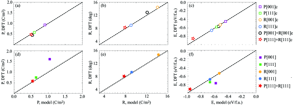
Figure 3: Structural properties and energies of BiFeO₃ polymorphs predicted using the Landau-like potential and plotted versus their corresponding DFT values. The top row shows the results obtained for the polymorphs with fixed cubic supercell (no strain), while the bottom row shows the properties of the polymorphs with fully relaxed cells. Panels (a) and (d) show the electric polarization $P$, (b) and (e) the FeO₆ octahedral rotations $R$, (c) and (f) the energies $E$. The polymorph P[001]+R[001] is not shown in panels (d) - (f), since its fully relaxed structure has very small FeO₆ octahedral rotations ($R=0.066^{o}$) and our model predicts it to be zero, therefore reducing to the state P[001].

Next, we consider the BiFeO₃ polymorphs with allowed strain relaxation (Figs. 3(d)-(f)). In this case, our potential also provides accurate predictions for all considered quantities for the most of the considered polymorphs; in particular, it yields the correct ground state of BiFeO₃ (P[111]+R[111]). There is only one polyrmorph for which the model is less accurate, namely, P[001]. In this case, the DFT optimized structure has a large distortion along the $z$ axis (the $c/a$ ratio is approximately 1.27), accompanied by a large $P_{z}$; this is usually called supertetragonal phase Béa et al. (2009); Zeches et al. (2009). This behavior is not well captured by our potential, as it underestimates the polarization and strains components compared to the DFT values ($P_{z}=1.039$ versus 1.624 C/m²; $\eta_{xx}=-0.012$ versus $-0.044$; $\eta_{zz}=0.065$ versus 0.216). This issue is also reflected in the energy predicted for this phase. From the DFT results one can see that, among the polymorphs with only polar distortion, the strain relaxation stabilizes the supertetragonal phase over the rhombohedral one (P[001] is lower than P[111] by 0.023 eV/f.u). Our model does predict the energy lowering of P[001] state due to the strain relaxation (the negative $\gamma_{P111}$ coupling results in large $P_{z}$ and $\eta_{zz}$). However, since it underestimates $P_{z}$ and $\eta_{zz}$, this energy reduction is not enough to stabilize P[001] over P[111]. Note that these deficiencies were to be expected, as we decided to use a minimal amount of DFT information on the supertetragonal phase when deriving the parameters of our model (see Table 2), because this state is not relevant for our ultimate purpose of studying polarization switching in the rhombohedral phase of BiFeO₃. Moreover, we checked that, if we try to capture the supertetragonal $c/a$, this makes it difficult to obtain a correct prediction for the ground state, as the P[001] state tends to become dominant.

IV.2 La_0.25Bi_0.75FeO₃

Now we discuss the case of La_0.25Bi_0.75FeO₃. We first compute the parameters of the potential using the analytical expressions in Sec. III.2.2. The resulting values are presented in Table 3. Next, we compare the model predictions and DFT values for our considered polymorphs in Fig. 4 (these results are also summarized in Table S2 of the Supplementary Material, together with the corresponding strains).

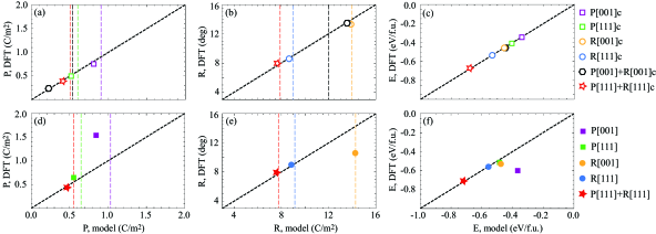
Figure 4: Structural properties and energies of La_0.25Bi_0.75FeO₃ polymorphs predicted using the Landau-like potential and plotted versus their corresponding DFT values. The top row shows the results obtained for the polymorphs with fixed cubic supercell (no strain), while the bottom row shows the properties of the polymorphs with fully relaxed cells. Panels (a) and (d) show the electric polarization $P$, (b) and (e) the FeO₆ octahedral rotations $R$, (c) and (f) the energies $E$. The polymorph P[001]+R[001] is not shown in panels (d) - (f), since its fully relaxed structure has very small FeO₆ octahedral rotations ($R=0.006^{o}$) and our model predicts it to be zero, therefore reducing to the state P[001]. The vertical dashed lines in panels (a), (b), (d) and (e) indicate the corresponding quantities for pure BiFeO₃.

Let us first consider the polymorphs with fixed cubic cell (Fig. 4(a)-(c)). Our potential provides very accurate predictions for polarizations and tilts, similarly to the case of pure BiFeO₃. The energy and relative stability of these polymorphs is also well captured by the model. Indeed, for polar-only structures both the model and DFT predict the rhombohedral P[111]c state to be lower in energy than the tetragonal P[001]c phase. The same holds for the polymorphs having only FeO₆ rotations: R[111]c is lower in energy than R[001]c. Note that the energy difference between the structures with tetragonal and rhombohedral phases are reduced compared to the case of pure BiFeO₃. The lowest-energy phase is P[111]+R[111]c, where polarization and tilts coexist.

For the polymorphs in which shape and volume of the cell are allowed to relax, we observe the following. First, the model predicts accurate values of the polarization in all cases except for P[001]. Indeed, for the supertetragonal state, the predicted $P_{s}$ and $\eta_{zz}$ are underestimated relative to the DFT values. This issue is also reflected in the energy of the polymorph: our potential predicts P[001] to be the highest-energy state, while DFT shows that this phase is the second-lowest in energy, right above the P[111]+R[111] ground state. Additionally, we find that the tilts are accurately predicted by our model for all polymorphs except R[001]; in that case, the tilt amplitude and the strains are exaggerated compared to the DFT values. Note that, as it was the case for pure BiFeO₃, these deficiencies are the result of the limited amount of DFT information on states P[001] and R[001] that was used to derive the parameters of our model.

IV.3 Intermediate compositions

In this section we demonstrate how our potentials can be used to study La_1-xBi_xFeO₃ with intermediate La content, $0<x<0.25$. We focus on the case of La_0.125Bi_0.875FeO₃ and check whether the properties of the polymorphs from the training set can be predicted by linear interpolation between BiFeO₃ and La_0.25Bi_0.75FeO₃.

We consider two types of interpolation. First, we construct a model for $x=0.125$ with coefficients obtained from interpolation of the corresponding values for the $x=0$ and $x=0.25$ cases. Using this model, we can easily predict the properties ($P_{s}$, $R_{s}$ and $E_{s}$) of all the polymorhps in the training set. Second, we derive the very same properties by direct interpolation of the values obtained at $x=0$ and $x=0.25$. In Fig. 5 we compare the quantities thus obtained, and also include the corresponding DFT values for the polymorphs for which the information is available (see figure caption). We find that both interpolation approaches yield very similar preditions. Further, the agreement with DFT is good except for the supertetragonal P[001] phase, where our predictions suffer from the issues discussed above. Hence, we conclude that our models give us a way to treat compounds with intermediate compositions.

V Discussion

Let us now discuss the physical insights that our models provide.

V.1 P-R coupling

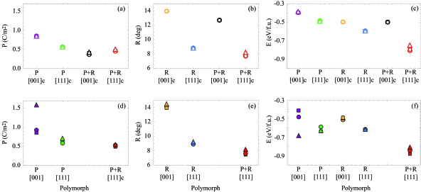
Figure 5: Structural properties and energies of La_0.125Bi_0.875FeO₃ polymorphs. Squares show the model predictions for $P$, $R$ and $E$ obtained using the interpolated potential’s coefficients, circles - the values obtained by direct interpolation of the corresponding results between pure BiFeO₃ and La_0.25Bi_0.75FeO₃, triangles - DFT values. The top row shows the results for fixed cubic cell (no strain), the bottom row - the results after a full strain relaxation. Panels (a) and (d) show the electric polarization $P$, (b) and (e) the FeO₆ octahedral rotations $R$, (c) and (f) the energies $E$. A missing DFT data point in the plot means that the structure of the corresponding polymorph developed non-negligible additional distortions during the DFT optimization, as described in Sec. III.2.1.

As it is well known from both experiments and computations, and correctly captured by our models, the ground state of BiFeO₃ has rhombohedral symmetry with $\mathbf{P}\parallel[111]$ and $\mathbf{R}\parallel[111]$. It is interesting to note, though, that the DFT energy of the polar-only BiFeO₃ polymorph P[001] is lower than that of P[111]. By contrast, among the polymorphs having only FeO₆ octahedral tilts, R[111] is the lowest-energy structure. These observations yield one important conclusion: that the rhombohedral symmetry of the BiFeO₃’s ground state critically depends on the presence of the octahedral tilts, as in their absence the material would be tetragonal.

In order to understand how the rhombohedral ground state of BiFeO₃ comes about, we consider the $F(P,R)$ part of our potential (Eq. 5) describing the coupling between polarization and octahedral rotations. The second term in Eq. (5), with $C_{PR}<0$ (see Table 3), favors states where $\mathbf{P}$ and $\mathbf{R}$ are along/about any $\langle 111\rangle$ direction, as for example, $\mathbf{P}\parallel[111]$ and $\mathbf{R}\parallel[\bar{1}1\bar{1}]$. In turn, the third term, with $C^{\prime}_{PR}<0$, favors phases where the FeO₆ tilts are about the axis defined by the polarization. Overall, these couplings lead $\mathbf{P}$ and $\mathbf{R}$ to appear together and aligned along/about the same $\langle 111\rangle$ direction. Thus, these are the interactions driving the stabilization of the ground state phase of BiFeO₃, rhombohedral and with co-existing polarization and tilts.

Does this mean, however, that $\mathbf{P}$ and $\mathbf{R}$ cooperate in BiFeO₃? We address this question by considering the energy diagram presented in Fig. 6. Here we show the energies of the P[111]c, R[111]c, and P[111]+R[111]c polymorphs as given by our model ($E_{2c}$, $E_{4c}$ and $E_{6c}$, respectively, see Table 4). We also show the energy of a virtual state in which $\mathbf{P}\parallel[111]$ coexists with $\mathbf{R}\parallel[111]$ but where these order parameters are not coupled. The energy of this virtual state is simply given by $E_{2c}+E_{4c}$, taking the cubic phase as the zero of energy. Clearly, the P[111]+R[111]c polymorph is higher in energy than the non-interacting virtual state and their energy difference arises from the coupling between $\mathbf{P}$ and $\mathbf{R}$ in P[111]+R[111]c structure. To understand this, we again consider the term $F(P,R)$ (Eq. 5) with the corresponding coefficients $B_{PR}$, $C_{PR}$ and $C^{\prime}_{PR}$ presented in Table 3 for BiFeO₃. For the polymorph P[111]+R[111]c, we have $P_{x}=P_{y}=P_{z}=P_{6c}$ and $R_{x}=R_{y}=R_{z}=R_{6c}$; therefore, $F_{6c}(P,R)=3(3B_{PR}+C_{PR}+C^{\prime}_{PR})P_{6c}^{2}R_{6c}^{2}$ for this state. In this expression, $3B_{PR}>0$ dominates over $C_{PR}+C^{\prime}_{PR}<0$ and leads to a ground state energy that is higher than that of the virtual non-interacting state.

Thus, we find that, overall, the $\mathbf{P}$ and $\mathbf{R}$ order parameters compete in BiFeO₃ ($B_{PR}>0$ dominates). Nevertheless, the polar and tilt instabilities are so strong that this repulsive interaction is not enough to prevent them from occurring simultaneously. Further, the $\mathbf{P}$-$\mathbf{R}$ competition is minimized when the order parameters are oriented along/about the same $\langle 111\rangle$ axis ($C_{PR},C^{\prime}_{PR}<0$), which yields the rhombohedral ground state phase of BiFeO₃.

V.2 Effects of La doping

Let us first consider how La doping affects the electric polarization. From Figs. 4(a) and 4(d) one can see that, for all considered polar polymorphs in the training set, a 25% La doping leads to reduction of $P$. Indeed, for the polymorphs with fixed cubic cell (Fig. 4(a)) we obtain a reduction of $P$ by $11-19\%$ for P[001]c, P[111]c and P[111]+R[111]c, and an even larger reduction for P[001]+R[001]c ($\approx 59\%$). When we allow the cell to relax (Fig. 4(d)), the obtained $P$ reduction is in the range of $5-20\%$.

Next, let us turn to the effect of La doping on the FeO₆ octahedral tilts. As one can see from Figs. 4(b) and 4(e), the presence of 25% La has a relatively small effect (reduction) in the amplitude of tilts. More precisely, we find that the R[001]c, R[111]c and P[111]+R[111]c polymorphs with fixed cubic cell present $1-4\%$ smaller $R$ compared to pure BiFeO₃. The exception is the P[001]+R[001]c state, where La doping leads to an increase in $R$ by 12%. Finally, when we allow the cell to relax, we find a $0.06-4\%$ reduction of $R$ in all considered polymorphs.

Table 4: Energies $E_{s}$ of BiFeO₃ polymorphs calculated using DFT and predicted by the Landau-like potential introduced in this work (the coefficents of the potential are obtained using the analytical approach described in Sec. III.2.2). Energy values are relative to the energy of the reference cubic phase and given in eV per 5-atom unit cell.

Polymorph		$E_{s}$ (DFT)	$E_{s}$ (Model)
1c	P[001]c	-0.445	-0.445
2c	P[111]c	-0.580	-0.580
3c	R[001]c	-0.527	-0.527
4c	R[111]c	-0.651	-0.650
5c	P[001]+R[001]c	-0.556	-0.546
6c	P[111]+R[111]c	-0.853	-0.919
1	P[001]	-0.764	-0.589
2	P[111]	-0.741	-0.677
3	R[001]	-0.536	-0.540
4	R[111]	-0.679	-0.671
5	P[001]+R[001]	-0.764	-0.593
6	P[111]+R[111]	-0.909	-0.967

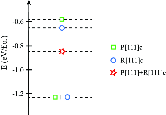
Figure 6: Model energies of several BiFeO₃ polymorphs. The lowest energy configuration corresponds to the virtual state in which $\mathbf{P}\parallel[111]$ and $\mathbf{R}\parallel[111]$ coexist but are not coupled (see text).

Our models allow us to rationalize the most important results described above. Let us start by noting that the $\mathbf{P}$-$\mathbf{R}$ couplings ($B_{PR}$, $C_{PR}$ and $C_{PR}^{\prime}$ in $F(P,R)$) are not significantly affected by the doping. Hence, they do not play a significant role to explain the La-induced effects.

Indeed, the effects of La doping on the polarization are essentially captured by the changes in the $F(P)$ term of the potential (Eq. 2). As shown in Table 3, we find that $A_{P}$ (quadratic coupling) is reduced in magnitude upon doping, indicating a weaker ferroelectric instability of the cubic phase. Additionally, both $B_{P}$ and $C_{P}$ increase and the relevant combination, $3B_{P}+C_{P}>0$, becomes larger; hence, the quartic couplings have a stronger effect on the energy landscape compared to pure BiFeO₃. All these changes cooperate to yield shallower ferroelectric energy wells associated to $F(P)$ for La-doped BiFeO₃, with smaller equlibrium polarization and lower energy barrier between states of opposite $\mathbf{P}$. Note that this is consistent with previous studies on the effect of La-doping on the switching characteristics of BiFeO₃ Prasad et al. (2020); Parsonnet et al. (2020).

As regards the tilt energy given by $F(R)$, Table 3 shows that the presence of La weakens the cubic-phase instability ($A_{R}$ becomes less negative); by contrast, the quartic term ($3B_{R}+C_{R}>0$) gets reduced upon doping, thus favoring larger tilts. These changes oppose each other, and result in the generally observed moderate reduction in the amplitude of the FeO₆ rotations.

Finally, as shown in Fig. 4, the P[001]+R[001]c case is peculiar, as it presents the largest reduction in $P$ (about 59 %) and is the only one displaying an increase of $R$ (about 12 %). We can rationalize this result by noting that, for this state, the quartic part of the energy in $F(P)$ (resp. $F(R)$) is controlled by the $B_{P}$ (resp. $B_{R}$) coupling alone. Upon doping $B_{P}$ grows ($B_{R}$ decreases), which favors smaller polarizations (larger tilts). Further, because of the strong competition between polarization and tilts in tetragonal states ($B_{PR}>0$; $C_{PR}$ and $C^{\prime}_{PR}$ do not contribute), the changes get particularly large in the case of P[001]+R[001]c. Note also a subtle difference between P[001]+R[001]c and P[111]+R[111]c. In the latter case, the relevant quartic parameter for the tilts is $3B_{R}+C_{R}$, and the La-induced decrease in $B_{R}$ is partly compensated by the increase in $C_{R}$; as a result, the tilts do not grow at all (recall $A_{R}<0$ grows upon doping) and the decrease of the polarization is relatively small.

Note that all these observations are consistent with what we know about the atomistic origin of the polar and tilt instabilities in BiFeO₃. The former rely on the presence of stereochemically active $6s$ lone pairs in the Bi³⁺ cations; hence, their partial substitution by lone-pair-free La cations naturally leads to smaller polarizations. The latter are mainly controlled by the ionic radius of the Bi³⁺ cation; since La³⁺ is similar in size, the doping leaves $R$ largely unaffected.

VI Conclusions

In summary, we have introduced the simplest, lowest-order Landau-like potential for BiFeO₃ and related compounds, as well as methods that allow to compute the potential parameters from Density Functional Theory (DFT). More precisely, we have derived analytical expressions for all the model coefficients as functions of the energies and structural features (polarization, FeO₆ octahedral tilts and strains) of a small set of relevant polymorphs. We have applied the proposed approach to BiFeO₃ and La_0.25Bi_0.75FeO₃, showing its overall accuracy in reproducing the DFT data. We have also showed that our models can be used – by interpolation – to predict the properties of compounds with intermediate dopant concentrations. We note that the introduced potential, as well as the analytical scheme to obtain its coefficients from DFT, can be readily applied to study the properties of other perovskite oxides characterized by the same order parameters (polarization, antiphase oxygen-octahedral tilts, strains). This includes ferroelectrics where the tilts are not important (e.g., BaTiO₃ or PbTiO₃), antiferrodistortive non-polar perovskites (e.g., LaAlO₃), or compounds where both distortions play a relevant role (e.g., SrTiO₃), as well as their corresponding solid solutions. In principle, an extension of our scheme to compounds where other order parameters are relevant (e.g., in-phase tilts in orthorhombic perovskites like CaTiO₃ Chen et al. (2018)) should be straightforward.

VII Acknowledgements

We thank John M. Mangeri for the fruitful discussions. Work funded by the the Semiconductor Research Corporation and Intel via contract no. 2018-IN-2865. We also acknowledge the support of the Luxembourg National Research Fund through Grant FNR/C18/MS/12705883/REFOX/Gonzalez.

References

- Spaldin and Fiebig (2005) N. A. Spaldin and M. Fiebig, Science 309, 391 (2005).
- Eerenstein et al. (2006) W. Eerenstein, N. D. Mathur, and J. F. Scott, Nature 442, 759 (2006), ISSN 1476-4687.
- Catalan and Scott (2009) G. Catalan and J. F. Scott, Advanced Materials 21, 2463 (2009).
- Moreau et al. (1971) J. Moreau, C. Michel, R. Gerson, and W. James, Journal of Physics and Chemistry of Solids 32, 1315 (1971), ISSN 0022-3697.
- Smith et al. (1968) R. T. Smith, G. D. Achenbach, R. Gerson, and W. J. James, Journal of Applied Physics 39, 70 (1968).
- Michel et al. (1969) C. Michel, J.-M. Moreau, G. D. Achenbach, R. Gerson, and W. James, Solid State Communications 7, 701 (1969), ISSN 0038-1098.
- Kubel and Schmid (1990) F. Kubel and H. Schmid, Acta Crystallographica Section B 46, 698 (1990).
- Seshadri and Hill (2001) R. Seshadri and N. A. Hill, Chemistry of Materials 13, 2892 (2001), ISSN 0897-4756.
- Lebeugle et al. (2007) D. Lebeugle, D. Colson, A. Forget, and M. Viret, Applied Physics Letters 91, 022907 (2007).
- Wang et al. (2003) J. Wang, J. B. Neaton, H. Zheng, V. Nagarajan, S. B. Ogale, B. Liu, D. Viehland, V. Vaithyanathan, D. G. Schlom, U. V. Waghmare, et al., Science 299, 1719 (2003), ISSN 0036-8075.
- Glazer (1972) A. M. Glazer, Acta Crystallographica Section B 28, 3384 (1972).
- Ederer and Spaldin (2005) C. Ederer and N. A. Spaldin, Phys. Rev. Lett. 95, 257601 (2005).
- Diéguez et al. (2011) O. Diéguez, O. E. González-Vázquez, J. C. Wojdeł, and J. Íñiguez, Phys. Rev. B 83, 094105 (2011).
- Bhide and Multani (1965) V. Bhide and M. Multani, Solid State Communications 3, 271 (1965), ISSN 0038-1098.
- Dzyaloshinsky (1958) I. Dzyaloshinsky, Journal of Physics and Chemistry of Solids 4, 241 (1958), ISSN 0022-3697.
- Moriya (1960) T. Moriya, Phys. Rev. 120, 91 (1960).
- Sosnowska et al. (1982) I. Sosnowska, T. P. Neumaier, and E. Steichele, Journal of Physics C: Solid State Physics 15, 4835 (1982).
- Sosnowska et al. (2002) I. Sosnowska, W. Schäfer, W. Kockelmann, K. H. Andersen, and I. O. Troyanchuk, Applied Physics A 74, s1040 (2002), ISSN 1432-0630.
- Bai et al. (2005) F. Bai, J. Wang, M. Wuttig, J. Li, N. Wang, A. P. Pyatakov, A. K. Zvezdin, L. E. Cross, and D. Viehland, Applied Physics Letters 86, 032511 (2005).
- Béa et al. (2007) H. Béa, M. Bibes, S. Petit, J. Kreisel, and A. Barthélémy, Philosophical Magazine Letters 87, 165 (2007).
- Sando et al. (2013) D. Sando, A. Agbelele, D. Rahmedov, J. Liu, P. Rovillain, C. Toulouse, I. C. Infante, A. P. Pyatakov, S. Fusil, E. Jacquet, et al., Nature Materials 12, 641 (2013), ISSN 1476-4660.
- Heron et al. (2014) J. T. Heron, J. L. Bosse, Q. He, Y. Gao, M. Trassin, L. Ye, J. D. Clarkson, C. Wang, J. Liu, S. Salahuddin, et al., Nature 516, 370 (2014), ISSN 1476-4687.
- Manipatruni et al. (2018) S. Manipatruni, D. E. Nikonov, and I. A. Young, Nature Physics 14, 338 (2018), ISSN 1745-2481.
- Prasad et al. (2020) B. Prasad, Y.-L. Huang, R. V. Chopdekar, Z. Chen, J. Steffes, S. Das, Q. Li, M. Yang, C.-C. Lin, T. Gosavi, et al., Advanced Materials 32, 2001943 (2020).
- Chu et al. (2008) Y. H. Chu, Q. Zhan, C.-H. Yang, M. P. Cruz, L. W. Martin, T. Zhao, P. Yu, R. Ramesh, P. T. Joseph, I. N. Lin, et al., Applied Physics Letters 92, 102909 (2008).
- González-Vázquez et al. (2012) O. E. González-Vázquez, J. C. Wojdeł, O. Diéguez, and J. Íñiguez, Phys. Rev. B 85, 064119 (2012).
- Zhang et al. (2019) L. Zhang, Y.-L. Huang, G. Velarde, A. Ghosh, S. Pandya, D. Garcia, R. Ramesh, and L. W. Martin, APL Materials 7, 111111 (2019).
- Parsonnet et al. (2020) E. Parsonnet, Y.-L. Huang, T. Gosavi, A. Qualls, D. Nikonov, C.-C. Lin, I. Young, J. Bokor, L. W. Martin, and R. Ramesh, Phys. Rev. Lett. 125, 067601 (2020).
- Landau (1937a) L. D. Landau, Journal of Experimantal and Theoretical Physics 7, 19 (1937a).
- Landau (1937b) L. D. Landau, Journal of Experimantal and Theoretical Physics 7, 627 (1937b).
- Devonshire (1949) A. Devonshire, The London, Edinburgh, and Dublin Philosophical Magazine and Journal of Science 40, 1040 (1949).
- Devonshire (1951) A. Devonshire, The London, Edinburgh, and Dublin Philosophical Magazine and Journal of Science 42, 1065 (1951).
- Umantsev (2012) A. Umantsev, Field Theoretic Method in Phase Transformations (Springer New York, Dordrecht, Heidelberg, London, 2012).
- K. M. Rabe (2007) J.-M. T. K. M. Rabe, C. H. Ahn, Physics of Ferroelectrics. A Modern Perspective (Springer, Berlin, Heidelberg, 2007).
- Hohenberg and Kohn (1964) P. Hohenberg and W. Kohn, Phys. Rev. 136, B864 (1964).
- Kohn and Sham (1965) W. Kohn and L. J. Sham, Phys. Rev. 140, A1133 (1965).
- Kresse and Furthmüller (1996) G. Kresse and J. Furthmüller, Phys. Rev. B 54, 11169 (1996).
- Perdew et al. (2008) J. P. Perdew, A. Ruzsinszky, G. I. Csonka, O. A. Vydrov, G. E. Scuseria, L. A. Constantin, X. Zhou, and K. Burke, Phys. Rev. Lett. 100, 136406 (2008).
- Dudarev et al. (1998) S. L. Dudarev, G. A. Botton, S. Y. Savrasov, C. J. Humphreys, and A. P. Sutton, Phys. Rev. B 57, 1505 (1998).
- Blöchl (1994) P. E. Blöchl, Phys. Rev. B 50, 17953 (1994).
- Le Page and Saxe (2002) Y. Le Page and P. Saxe, Phys. Rev. B 65, 104104 (2002).
- Marton et al. (2017) P. Marton, A. Klíč, M. Paściak, and J. Hlinka, Phys. Rev. B 96, 174110 (2017).
- Béa et al. (2009) H. Béa, B. Dupé, S. Fusil, R. Mattana, E. Jacquet, B. Warot-Fonrose, F. Wilhelm, A. Rogalev, S. Petit, V. Cros, et al., Phys. Rev. Lett. 102, 217603 (2009).
- Zeches et al. (2009) R. J. Zeches, M. D. Rossell, J. X. Zhang, A. J. Hatt, Q. He, C.-H. Yang, A. Kumar, C. H. Wang, A. Melville, C. Adamo, et al., Science 326, 977 (2009).
- Chen et al. (2018) P. Chen, M. N. Grisolia, H. J. Zhao, O. E. González-Vázquez, L. Bellaiche, M. Bibes, B.-G. Liu, and J. Íñiguez, Phys. Rev. B 97, 024113 (2018).