Kinematics and Metallicity of Red Giant Branch Stars in the Northeast Shelf of M31

Abstract

We obtained Keck/DEIMOS spectra of 556 individual red giant branch stars in 4 spectroscopic fields spanning $13-31$ projected kpc along the Northeast (NE) shelf of M31. We present the first detection of a complete wedge pattern in the space of projected M31-centric radial distance versus line-of-sight velocity for this feature, which includes the returning stream component of the shelf. This wedge pattern agrees with expectations of a tidal shell formed in a radial merger and provides strong evidence in favor of predictions of Giant Stellar Stream (GSS) formation models in which the NE shelf originates from the second orbital wrap of the tidal debris. The observed concentric wedge patterns of the NE, West (W), and Southeast (SE) shelves corroborates this interpretation independently of the models. We do not detect a kinematical signature in the NE shelf region corresponding to an intact progenitor core, favoring GSS formation models in which the progenitor is completely disrupted. The shelf’s photometric metallicity ([Fe/H]_phot) distribution implies that it is dominated by tidal material, as opposed to the phase-mixed stellar halo or the disk. The metallicity distribution ([Fe/H]_phot = $-0.42$ $\pm$ $0.01$) also matches the GSS, and consequently the W and SE shelves, further supporting a direct physical association between the tidal features.

1 Introduction

In the hierarchical assembly paradigm, galaxy mergers play an essential role in driving the formation and growth of galaxies (e.g., White & Rees 1978). The tidal relics of these merger events encode a wealth of information concerning the accretion history of the host galaxy (e.g., Bullock & Johnston 2005; Johnston et al. 2008), particularly in the form of stellar streams and shells (Hernquist & Quinn, 1988; Johnston et al., 2001; Hendel & Johnston, 2015). The dynamics of streams and shells can also serve as powerful probes of the host galaxy gravitational potential (Merrifield & Kuijken, 1998; Ebrová et al., 2012; Sanderson & Helmi, 2013; Law & Majewski, 2010; Fardal et al., 2013).

The Milky Way (MW) provides ample evidence for ongoing tidal disruption in the form of the Sagittarius stream (Ibata et al., 2001), a plethora of smaller streams (Helmi 2020 and references therein), and potentially shell-like overdensities (Belokurov et al., 2007; Jurić et al., 2008) that may originate from a radial merger (Simion et al., 2018, 2019; Donlon et al., 2019, 2020; Naidu et al., 2021). Deep, wide-field imaging surveys of massive galaxies beyond the Local Group have revealed rich collections of large-scale tidal features (including shells) surrounding both spirals and ellipticals (e.g., Tal et al. 2009; Martínez-Delgado et al. 2010, 2021b; Atkinson et al. 2013; Kado-Fong et al. 2018). However, since these low surface brightness features are intrinsically difficult to detect for large samples of external galaxies, many studies have focused on the resolved stellar populations of features in individual nearby galaxies (e.g., Mouhcine et al. 2010; Ibata et al. 2014; Okamoto et al. 2015; Crnojević et al. 2016; Martínez-Delgado et al. 2021a). Studies of kinematical tracers probing tidal debris are even more challenging and have thus been limited to a handful of external galaxies (e.g., Romanowsky et al. 2012; Foster et al. 2014).

Owing to its proximity ($d_{\rm M31}$ = 773 kpc; Conn et al. 2016), the Andromeda galaxy (M31) presents a rare opportunity for detailed photometric and spectroscopic studies of resolved stars in tidal structures. M31 possesses a metal-rich giant stellar stream (GSS; Ibata et al. 2001) in the southern portion of its stellar halo and a diffuse shelf-like overdensity in the northeast (NE) with red colors similar to the GSS (Ferguson et al., 2002). Fardal et al. (2007) detected a second shelf in the west (W) using the Ferguson et al. imaging and Gilbert et al. (2007) identified a third faint shelf in the southeast (SE) via spectroscopy. The chemical similarity of red giant branch (RGB) stars in the W and SE shelves to the GSS (Gilbert et al., 2007; Fardal et al., 2012) as well as the striking consistency between various stellar populations in the NE, W, and SE shelves and the GSS (Brown et al., 2006, 2008; Ferguson et al., 2005; Richardson et al., 2008; Tanaka et al., 2010; Bernard et al., 2015) support the hypothesis that these structures form a related system of tidal debris. The luminosity functions of planetary nebulae (PNe) in M31 additionally support a common origin for the NE shelf and GSS, while constraints for the W shelf are limited but suggest it is distinct from the disk (Bhattacharya et al., 2019, 2021). However, kinematical and chemical information in the NE shelf is necessary to finally confirm the putative association between the shelves and the GSS.

Orbital models for the formation of the GSS in a minor merger ($M_{\star}\sim(1-5)\times 10^{9}M_{\odot}$) predict that the shelves correspond to tidal debris from the distinct progenitor of the GSS (Fardal et al., 2006, 2007, 2008, 2013; Mori & Rich, 2008; Sadoun et al., 2014; Miki et al., 2016; Kirihara et al., 2014, 2017). In these models, the NE shelf is composed of material from the second pericentric passage of the disrupting progenitor as well as the forward continuation of the GSS. The models place the central material of the progenitor in the NE shelf region and allow for the presence of an intact GSS progenitor core based on its initial central density (e.g., Fardal et al. 2013; Kirihara et al. 2017), although no such structure has yet been detected (cf. Dorman et al. 2012; Davidge 2012). Major merger models ($M_{\star}\sim 10^{10}M_{\odot}$) can similarly form tidal structures resembling the GSS and shelves (Hammer et al., 2018; D’Souza & Bell, 2018), but have not yet been shown to reproduce the shelves at the level of detail provided by minor merger models.

Despite not explicitly fitting for the detailed properties of the shelves, the Fardal et al. minor merger models have predicted the existence of the SE shelf (Fardal et al., 2007; Gilbert et al., 2007) and show excellent agreement with the kinematics of RGB stars in the W shelf (Fardal et al., 2012). These successes appear to be natural consequences of the constraints placed on the merger scenario using spatial and kinematical observations of the GSS (McConnachie et al., 2003; Ibata et al., 2004; Gilbert et al., 2009) and stellar surface density maps of M31 (Ibata et al., 2001; Ferguson et al., 2002; Irwin et al., 2005), where the orbital trajectory of the progenitor is only loosely required to pass through the location of the NE shelf. Moreover, Fardal et al. (2013) demonstrated that the predicted kinematical signature for the NE shelf partially overlaps with a small sample of PNe that form an apparent stream near the shelf (Merrett et al., 2003, 2006).

Detailed kinematics for a large sample of RGB stars in the NE shelf could conclusively establish that it is indeed a tidal shell, place stringent constraints on GSS merger scenarios, identify whether an intact GSS progenitor core exists, and probe M31’s gravitational potential at the location of the shelf. Furthermore, the NE shelf metallicity distribution could be used to infer the properties of the progenitor as the shelf region is predicted to contain its metal-rich central debris (Mori & Rich, 2008; Fardal et al., 2008; Miki et al., 2016; Kirihara et al., 2017). The observed metallicity gradient(s) in the GSS (Ibata et al., 2007; Gilbert et al., 2009; Conn et al., 2016; Cohen et al., 2018; Escala et al., 2021) could be combined with the metallicity distributions of the NE, W, and SE shelves to connect chemical variations on the sky to the intrinsic properties of the progenitor (Fardal et al., 2008; Miki et al., 2016; Kirihara et al., 2017; Milošević et al., 2022). This metallicity mapping may be crucial for distinguishing between major and minor merger scenarios for the formation of the GSS and shelves (see the discussions of Gilbert et al. 2019 and Escala et al. 2021).

In this work, we present the first analysis of the metallicity and kinematics of RGB stars in the NE shelf of M31. This contribution is part of the Spectroscopic and Photometric Landscape of Andromeda’s Stellar Halo survey (SPLASH; Guhathakurta et al. 2005; Gilbert et al. 2006), which has produced tens of thousands of Keck/DEIMOS spectra along lines-of-sight to M31’s halo, disk, and dwarf galaxies (e.g., Kalirai et al. 2010; Dorman et al. 2012, 2015; Gilbert et al. 2012, 2014; Tollerud et al. 2012). In Section 2, we introduce spectroscopic and photometric data for the NE shelf. We investigate the kinematics, metallicity, and projected phase space distribution of the NE shelf in Section 3. We perform detailed comparisons of the shelf’s observed properties to N-body models in Section 4 and the GSS and W and SE shelves as observed by SPLASH in Section 5. Lastly, we discuss results for the NE shelf in the context of the literature in Section 6 before summarizing in Section 7.

2 Data

2.1 Observations and Data Reduction

Table 1: Keck/DEIMOS Multi-Object Slitmask Observations in M31’s NE Shelf

Slitmask	Rproj
	R.A.	Decl.	Mask P.A.
	Obs. Date		(∘ E of N)
	texp
	Airmass	No.
	No.	Targetsa
	No.
	M31c
NE1	19.6	00:50:04.96	+41:39:53.3	30	2011 Nov 23	50.0	1.10	190	138	123
NE2	25.7	00:51:52.11	+42:02:22.3	30	2011 Nov 23	55.0	1.26	186	117	79
NE3	14.5	00:48:17.03	+41:26:33.6	30	2011 Nov 24	51.7	1.27	214	154	135
NE4	29.2	00:52:52.20	+42:15:44.8	30	2011 Nov 24	60.0	1.08	182	124	91
NE6	21.8	00:50:27.03	+41:56:32.8	40	2011 Nov 24	51.7	1.23	200	149	128

• Number of targets on the slitmask with successfully extracted one-dimensional spectra.

• Number of targets with successful radial velocity measurements (Section 2.1).

• Number of targets classified as M31 RGB stars (Section 3.1).

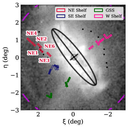
Figure 1: Location of the spectroscopic fields targeting the NE Shelf (red open boxes; Table 2.1, Section 2.1) in M31-centric coordinates overlaid on a star count map from the PAndAS survey (McConnachie et al., 2018). The approximate size and orientation of each DEIMOS field is represented by a 16’ $\times$ 4’ rectangle. We also show spectroscopic fields from the Elemental Abundances in M31 survey (filled boxes; Gilbert et al. 2019; Escala et al. 2020a, b) and fields previously observed as part of the SPLASH survey (open boxes; Kalirai et al. 2006; Gilbert et al. 2007, 2009; Fardal et al. 2012) spanning the SE Shelf (blue), W shelf (pink), and GSS (green). The black points are the edges of the NE and W shelves defined by Fardal et al. (2007) via applying an edge filter to the Irwin et al. (2005) star count map.

We observed five slitmasks targeting M31’s NE shelf with the DEIMOS instrument on Keck II as part of the SPLASH survey. We utilized the 1200 $\ell$/mm grating, which has a spectral dispersion of 0.33 Å pixel^-1, with the OG550 order blocking filter and a central wavelength of 7800 Å for our science configuration. The spectroscopic fields were observed in Fall 2011 with $\sim$1 hr exposures. Table 2.1 summarizes the observations. Figure 1 shows the locations of the NE shelf fields on the sky in M31-centric coordinates, overlaid on a star count map of RGB candidates from the Pan-Andromeda Archaeological Survey (PAndAS; McConnachie et al. 2018). The naming convention for the NE shelf fields indicates the order in which the masks were designed, rather than their radial distance from M31. We included reference DEIMOS fields from the Elemental Abudances in M31 survey (Gilbert et al., 2019; Escala et al., 2020a, b) and fields previously observed as part of the SPLASH survey (Kalirai et al., 2006; Gilbert et al., 2007, 2009; Fardal et al., 2012) targeting the SE shelf, W shelf, and GSS. Figure 1 also indicates the edges of the NE and W shelves defined by Fardal et al. (2007) via applying the Sobel operator to the Irwin et al. (2005) star map.

We extracted and reduced one-dimensional spectra from the two-dimensional images using a modified version of the spec2d software (Cooper et al., 2012; Newman et al., 2013) for stellar sources (Simon & Geha, 2007). The one-dimensional spectra were then cross-correlated against empirical templates of hot stars to shift them into the rest frame and measure radial velocities. We corrected the velocity measurements for slit miscentering using the A-band (Sohn et al., 2007) and transformed them into the heliocentric frame. As described by Howley et al. (2013), the total velocity uncertainty is determined by scaling the cross-correlation based error with a value determined from duplicate measurements of RGB stars at the distance of M31, and then adding in quadrature with a systematic velocity error of 2.2 km s^-1 computed by Simon & Geha (2007).

Using the visual inspection software zspec (D. Madgwick, DEEP2 survey), each spectrum was assigned a quality code ($Q$) for its radial velocity measurement. We restrict our analysis to objects with successful radial velocity measurements that match two or more strong spectral features ($Q=4$) or a combination of one strong spectral feature and additional marginal features ($Q=3$; Guhathakurta et al. 2006). The median total velocity uncertainty for stars with successful velocity measurements is 5.3 km s^-1. We excluded some targets with successful velocity measurements from the subsequent analysis because of missing spectral data at red wavelengths, which is necessary to evaluate membership (Section 3.1).

2.2 Photometry

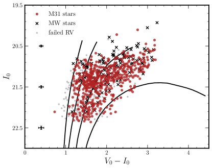
Figure 2: Extinction-corrected $(V_{0},I_{0})$ CMD (Section 2.2) for all stars in the NE shelf fields (Table 2.1), including stars without successful radial velocity measurements (gray points), MW foreground stars (black crosses; Section 3.1), and M31 RGB stars (red circles). The median photometric uncertainties as a function of magnitude are shown as black errorbars on the left. For reference, we show PARSEC isochrones (black lines; Marigo et al. 2017), assuming 12 Gyr ages and [$\alpha$/Fe] = 0, with [Fe/H] = $-2.0$, $-1.0$, $-0.5$, and $0$ (from left to right).

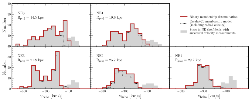
Figure 3: Heliocentric radial velocity distributions for stars with successful velocity measurements (grey filled histograms; Section 2.1) in spectroscopic fields targeting the NE shelf (Table 2.1), including both M31 RGB stars and MW foreground dwarf stars. From top to bottom and left to right, the fields probe larger M31-centric projected radii, approaching the “tip” of the tidal shell pattern (Section 3.4). The black dashed lines show the velocity distribution of stars classified as likely M31 members by the probabilistic model of Escala et al. (2020b), which includes radial velocity as a membership diagnostic. This model mistakenly classifies NE shelf stars in field NE3 with MW-like velocities ($v_{\rm helio}$ $\gtrsim-150$ km s^-1; Section 3.1) as likely MW contaminants. Thus, we assigned stars with $v_{\rm helio}$ $>-100$ ($-150$) km s^-1 for the inner (outer) fields or spectral signatures of strong Na I $\lambda$8190 absorption as MW contaminants (red open histograms; Section 3.1).

We sourced photometry from MegaCam images obtained in the $g^{\prime},i^{\prime}$ bands using the 3.6 m Canada-France-Hawaii Telescope (CFHT). The images were reduced with the CFHT MegaPipe pipeline (Gwyn, 2008) and the $g^{\prime}$, $i^{\prime}$ magnitudes were transformed to Johnson-Cousins $V,I$ using observations of Landolt photometric standard stars (Kalirai et al., 2006). When designing slitmasks, we identified RGB candidates based on only the $I$-band magnitude to avoid introducing bias into the target selection. This still yields low MW contamination (Section 3.1) in the NE shelf region owing to the high density of M31 stars relative to the foreground below the tip of the RGB at $I_{0}\sim 20.5$ magnitudes.

Figure 2 shows the de-reddened $V_{0},I_{0}$ CMD for all stars with successful radial velocity measurements (Section 2.1) in the NE shelf fields (Table 2.1). We corrected the photometry for the effects of dust extinction by assuming field-specific interstellar reddening values from the maps of Schlegel et al. (1998) and applying the corrections defined by Schlafly & Finkbeiner (2011). We also show PARSEC isochrones (Marigo et al., 2017) for reference, assuming an age of 12 Gyr, [$\alpha$/Fe] = 0, and $m-M$ = 24.47 for consistency with previous studies in the SPLASH collaboration. Based on this grid of theoretical isochrones, we determined [Fe/H]_phot via interpolation given the color and magnitude of each star (Escala et al., 2020a).

3 Properties of the Northeast Shelf

3.1 Membership

In prior studies of M31’s stellar halo, we employed likelihood-based methods (Gilbert et al., 2006; Escala et al., 2020b) to separate M31 RGB stars from the MW foreground using diagnostic measurements such as radial velocity ($v_{\rm helio}$), Na I $\lambda$8190 doublet equivalent width (EW_Na), photometric metallicity ([Fe/H]_phot), and calcium-triplet based metallicity ([Fe/H]_CaT). In particular, the technique of Escala et al. (2020b) relies on Bayesian inference to assign each target star a probability of M31 membership based on the observed properties of over a thousand M31 and MW stars securely identified in SPLASH (Gilbert et al., 2006, 2012). As a consequence, these methods were calibrated to the properties of the stellar halo in M31’s southeast quadrant, where known M31 substructure is not present at MW-like heliocentric velocities ($v_{\rm helio}$ $\gtrsim-150$ km s^-1; Gilbert et al. 2018). However, these approaches to membership determination overestimate the degree of MW contamination for the NE shelf fields when using radial velocity as a diagnostic.

For context, Figure 3 shows the heliocentric radial velocity distributions for stars in the NE shelf fields with successful velocity measurements, including both M31 RGB stars and intervening MW dwarf stars. In the innermost field NE3, the Escala et al. model assigns a low probability of M31 membership to a prominent kinematical feature at $v_{\rm helio}$ $\sim$ $-120$ km s^-1 (Figure 3) when including radial velocity as a diagnostic. However, this feature likely corresponds to the NE shelf based on its position and velocity (Section 3.4). When selecting stars in NE3 that have velocities consistent with this feature ($-190$ km s^-1 $<$ $v_{\rm helio}$ $<-100$ km s^-1), we found that their EW_Na and [Fe/H]_CaT measurements and CMD positions are consistent with those of stars in the NE shelf fields with M31-like velocities ($v_{\rm helio}$ $\lesssim$ $-$200 km s^-1; Figure 4). Thus, the likelihood-based M31 membership models are not uniformly applicable to the NE shelf fields when using radial velocity criteria due to the distinct kinematical structure of the NE shelf.

We adopted a binary membership determination in which we classified stars with clear spectral signatures of strong Na I $\lambda$8190 absorption or $v_{\rm helio}$ $>-100$ km s^-1 ($v_{\rm helio}$ $>-150$ km s^-1) for R_proj $<$ 20 kpc (R_proj $>$ 20 kpc) as belonging to the MW foreground. We relied on visual inspection of the Na I doublet as opposed to EW_Na measurements owing to the low S/N of the spectra. We do not detect stars with strong Na I absorption at M31-like velocities (Figure 4) given that MW contaminants in this velocity range are likely blue main sequence turn-off stars in the MW’s stellar halo.

The change in velocity cut with projected radius is a consequence of the shifting of the shelf velocity distribution relative to the constant MW foreground (Figure 3). The velocity cut includes the majority of stars in the NE3 velocity peak while excluding the majority of stars at MW-like velocities in this field. We characterized the MW velocity distribution over the NE shelf region as probed by our selection function by utilizing an expectation-maximization algorithm to fit a 3-component Gaussian mixture (Pedregosa et al. 2011) to the combined velocity distribution of the three outermost fields. We found $\mu_{v,{\rm MW}}=$ $-$62.6 km s^-1, $\sigma_{v,{\rm MW}}=$ 39.6 km s^-1, indicating that a velocity cut at $-$100 km s^-1 removes 82.8% of stars at MW-like velocities when assuming a normal distribution. In the outermost fields, the velocity cut should largely eliminate MW contamination, where Gilbert et al. (2007) found that MW dwarf stars along the line-of-sight to M31 are primarily limited to $v_{\rm helio}$ $>-150$ km s^-1.

Figure 4 shows [Fe/H]_phot, [Fe/H]_CaT, and EW_Na versus $v_{\rm helio}$ for stars classified as belonging to M31 and the MW in the NE shelf fields. The [Fe/H]_phot derivation (Section 2.2) assumes that stars are at the distance of M31 and the [Fe/H]_CaT calibration is appropriate only for RGB stars, therefore both are inaccurate for MW stars. We emphasize that we did not use selections on [Fe/H]_phot, [Fe/H]_CaT, or EW_Na measurements to determine membership. Instead, Figure 4 illustrates that a binary membership classification based solely on $v_{\rm helio}$ and apparent Na I absorption captures statistical differences between the observed properties of M31 and MW stellar populations, despite favoring completeness over lower contamination. For example, the median [Fe/H]_CaT and EW_Na of M31 (MW) stars is $-0.54$ ($-1.74$) and 1.7 (3.1) Å based on measurements with uncertainties $\delta$[Fe/H]_CaT $<$ 0.8 and $\delta$EW_Na $<$ 2 Å, respectively, which are consistent with known properties of M31 (MW) stars along the line-of-sight to M31 (Gilbert et al., 2006; Escala et al., 2020b). Table 2.1 provides the number of M31 RGB stars identified in each field.

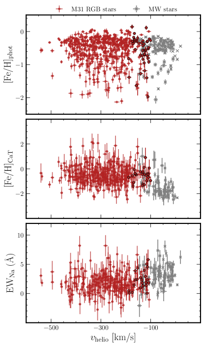
Figure 4: Photometric metallicity ([Fe/H]_phot; top), spectroscopic calcium-triplet based metallicity ([Fe/H]_CaT; middle), and the summed equivalent width of the Na I $\lambda$8190 doublet (EW_Na; bottom) versus heliocentric velocity for stars in the NE shelf fields (Table 2.1) classified as M31 RGB stars (red circles) and MW stars (gray crosses; Section 3.1). Stars in the NE3 velocity peak (Figure 3) are outlined in black. We show [Fe/H]_CaT (EW_Na) measurements with uncertainties $\delta$[Fe/H]_CaT $<$ 0.8 dex ($\delta$EW_Na $<$ 2 Å), where the large uncertainties are due to the low spectral S/N. Neither [Fe/H]_phot nor [Fe/H]_CaT are physically meaningful for MW stars but are useful as population diagnostics.

3.2 Empirical Modeling of the Velocity Distributions

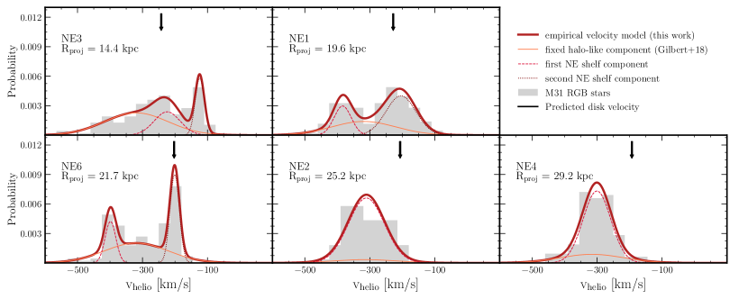
Figure 5: Heliocentric radial velocity distributions for M31 RGB stars (gray histograms; Section 3.1) in the NE shelf fields. We show the empirical velocity model derived for each field from the 50^th percentile values of the marginalized posterior probability distributions (thick red lines; Section 3.2, Table 3.2.2). We constructed the velocity models from a kinematically hot halo-like component with fixed mean and standard deviation (thin solid orange lines; Gilbert et al. 2018) and kinematically cold component(s) corresponding predominantly to NE shelf substructure (thin dotted and dashed red lines). We also show the median velocity of the disk predicted for each field assuming its presence (black arrows; Section 3.2.3).

The observed velocity distributions (Figure 3) clearly demonstrate that kinematical substructure is present across the spectroscopic fields. Such substructure is presumably associated with the tidal debris that constitutes the NE shelf. Thus, we performed empirically motivated modeling of the velocity distribution to identify probable substructure components directly from the data. This is in contrast to the N-body modeling used to predict the velocity structure of the NE shelf in Section 4.

3.2.1 Number of Kinematical Components

We confirmed that each field contains kinematical substructure by testing whether the velocity distributions for M31 RGB stars (Section 3.1) are consistent with a pure stellar halo component. We assumed that the stellar halo in the NE shelf region can be described by the kinematically unbiased parameterization found by Gilbert et al. (2018) for M31’s southeast quadrant via modeling the line-of-sight velocity distribution of over 5000 stars in radial bins spanning 9–175 projected kpc. We transformed the mean halo velocities in a given radial bin from the Galactocentric to heliocentric frame based on the median R.A. and Decl. of all stars in each NE shelf field. We performed an Anderson-Darling test with 10³ Monte Carlo trials to compare the observed velocity distribution of each field to the accompanying Gaussian stellar halo model. In each iteration, we randomly drew samples from the model according to the number of M31 members in each field (Table 2.1) and calculated the test statistic for a perturbation of the line-of-sight velocities assuming Gaussian measurement errors. We found that the velocity distribution for each field—including NE2 and NE4 despite the apparent lack of multiple velocity peaks—is highly inconsistent with a single kinematically hot stellar halo component.

To determine the number of kinematical components in each field, we used an expectation-maximization (EM) algorithm to fit Gaussian mixtures (Pedregosa et al., 2011) to the observed velocity distribution of M31 RGB stars. For each $N$-component model, we computed the Bayesian information criterion (BIC) for $10^{3}$ perturbations of the velocities according to their errors. We found that $N$-components = (2, 1, 3, 1, 2) minimizes the BIC for fields (NE1, NE2, NE3, NE4, NE6). However, the EM algorithm has no knowledge of the structural properties of the substructure-dominated NE shelf region and likely disregards the dynamically hot stellar halo that must be present at some level in each field. We therefore incremented the number of components by one to account for a kinematically hot halo-like component in each field except NE3.

As demonstrated by Figure 5, NE3 has a more complex velocity distribution, which makes the separation of substructure from a background halo-like component less straightforward. We evaluated whether NE3 contains 3 or 4 kinematical components when including a halo-like component (i.e., whether the field has 2 or 3 kinematically cold components) by modeling its velocity distribution using the procedure detailed in Section 3.2.2. We calculated a distribution of BICs using the models described by every 100^th sampled parameter combination from the converged portion of the flattened Markov chain assuming 3 and 4 components. Based on this, we concluded that a 3 component model composed of 2 substructure components and a halo-like component provides a better representation of the data for this field.

3.2.2 Sampling the Posterior Probability Distributions

Table 2: Empirical Velocity Distribution Model Parameters for NE Shelf Fields

Field	Rproj
	$\mu_{\rm halo}$
	$\sigma_{\rm halo}$
	$\mu_{\rm KCC1}$
	$\sigma_{\rm KCC1}$
	$f_{\rm KCC1}$
	$\mu_{\rm KCC2}$
	$\sigma_{\rm KCC2}$
	$f_{\rm KCC2}$
	(km/s)
NE3	14.4	$-$319.4	98.1	$-$224.3${}^{+20.3}_{-18.0}$	40.0${}^{+14.1}_{-15.4}$	0.24${}^{+0.11}_{-0.1}$	$-$123.7${}^{+3.9}_{-6.1}$	14.0${}^{+4.9}_{-2.9}$	0.20${}^{+0.05}_{-0.04}$
NE1	19.6	$-$319.0	98.1	$-$383.7${}^{+11.2}_{-10.2}$	26.4${}^{+9.7}_{-9.0}$	0.20${}^{+0.11}_{-0.09}$	$-$204.2${}^{+11.9}_{-10.5}$	45.9${}^{+7.7}_{-7.7}$	0.46${}^{+0.11}_{-0.12}$
NE6	21.7	$-$319.1	98.1	$-$398.6${}^{+7.1}_{-6.3}$	16.6${}^{+4.7}_{-3.8}$	0.18${}^{+0.05}_{-0.05}$	$-$200.9${}^{+3.0}_{-3.1}$	14.5${}^{+2.4}_{-2.1}$	0.33${}^{+0.05}_{-0.05}$
NE2	25.2	$-$316.2	98.0	$-$310.5${}^{+7.3}_{-7.4}$	55.4${}^{+5.2}_{-5.1}$	0.92${}^{+0.06}_{-0.14}$	…	…	…
NE4	29.2	$-$316.0	98.0	$-$300.6${}^{+6.2}_{-6.3}$	42.8${}^{+7.3}_{-6.3}$	0.79${}^{+0.12}_{-0.13}$	…	…	…

• Note. — The parameters describing the model components are mean velocity ($\mu$), velocity dispersion ($\sigma$), and normalized fractional contribution ($f$). We constructed each model from halo-like (Gilbert et al., 2018) and kinematically cold component(s) (KCCs) corresponding predominantly to NE shelf substructure (Section 3.2). The parameter values are the 50^th percentiles of the marginalized posterior probability distributions, where the errors are calculated from the 16^th and 84^th percentiles.

We modeled the observed velocity distribution in each field as a Gaussian mixture composed of kinematically cold components(s) that correspond to the NE shelf (see Section 3.2.3 for a discussion on the disk) and a kinematically hot halo-like component with fixed mean and dispersion but variable fractional contribution. We refer to the kinematically hot component as “halo-like” to emphasize that it may be composed of both a classical stellar halo (i.e., in-situ and phase-mixed accreted stars) and high-velocity-dispersion tidal debris constituting part of the shell. The log likelihood of this model is given by,

$$\ln\mathcal{L}=\sum_{i=1}^{N}\ln\left(\sum_{k=1}^{K}f_{k}\mathcal{N}(v_{i}|\mu_{k},\tau_{k}^{-1})\right),$$ (1)

where $i$ is the index representing a RGB star, $v_{i}$ is its heliocentric radial velocity, and $N$ is the number of RGB stars. $K$ is the total number of components (including the kinematically hot component), $k$ is the index for a given component, and $\mu_{k}$, $\tau_{k}=\sigma_{k}^{-2}$, and $f_{k}$ are the mean, inverse variance, and fractional contribution of each component. Note that the fractional contribution of the halo-like component is not a free parameter and is instead constrained by the kinematically cold component(s) (KCCs).

We sampled from the posterior distribution of the velocity model (Eq. 1) for each field using an affine-invariant Markov chain Monte Carlo (MCMC) ensemble sampler (emcee; Foreman-Mackey et al. 2013) with 10² walkers and $10^{4}$ steps. We limited the range of our model parameters to samples drawn from $-$600 km s^-1 $<\mu_{k}<$ $-$100 km s^-1, 5 km s^-1 $<$ $\sigma_{k}$ $<$ 150 km s^-1, and $0<f_{k}<1$, and required that $\mu_{k}<\mu_{k+1}$ and $\sum f_{k}\leq 1$ for KCCs. We implemented uniform priors on $\mu_{k}$ over the allowed range for maximal flexibility given the previously unstudied nature of the NE shelf velocity distribution for RGB stars. We assumed Gamma priors on $\tau_{k}$ with $\alpha$ = 2.25 and $\beta$ = 506.25 to penalize small values of $\sigma_{k}$ while enabling a lower probability extended tail toward high values of $\sigma_{k}$. We constructed the marginalized posterior distributions from the latter 50% of the samples, where Table 3.2.2 summarizes the model parameters calculated from the 16^th, 50^th, and 84^th percentiles of the posterior distributions.

Figure 5 shows the heliocentric velocity distributions for RGB stars in each field compared to its adopted velocity model. We also indicate the separate kinematically hot and cold components constituting the model in the figure. As previously discussed, the interior field NE3 has the most complicated velocity distribution, which is composed of a cold feature at $v_{\rm helio}$ $\sim$ $-120$ km s^-1 that is likely the upper envelope of the NE shelf (Section 3.4 and 4), a significant halo-like component, and a third component of unclear origin (c.f. Section 3.2.3). The fields at intermediate projected radii, NE1 and NE6, consist of two NE shelf components corresponding to the envelopes of the tidal shell (Section 3.4 and 4). The outermost fields, NE2 and NE4, are dominated by NE shelf substructure, where relatively insignificant halo-like components are favored by the model.

Based on the model for each field, we assigned each star a probability of belonging to substructure ($p_{\rm sub}$) given its heliocentric velocity. This probability is computed from the likelihood ratio between the KCC model(s) and halo-like component model. We emphasize that stars with lower values of $p_{\rm sub}$ may in fact belong to NE shelf substructure; $p_{\rm sub}$ should be interpreted as a measure of confidence that a star is associated with tidal debris based on velocity information alone.

3.2.3 Potential Contamination from M31’s Disk

We assessed whether a significant contribution from M31’s disk is expected in the NE shelf velocity distribution owing to its complex kinematical structure (Figure 5) and the proximity of the fields to the disk (Figure 1). Using a simple model for the perfectly circular rotation of an inclined disk (Guhathakurta et al., 1988) with inclination angle $i=77^{\circ}$ and position angle P.A. = 38^∘, we calculated the predicted line-of-sight velocities for a disk feature over the R.A., Decl. range (corresponding to R_disk = 28–42 kpc) spanned by our fields. Based on a rotation curve derived from HI kinematics out to R_disk = 38 kpc and corrected for the inclination of the disk (Chemin et al., 2009), the expected disk rotation velocity in the NE shelf fields is $\sim$250 km s^-1.

When using the simple model, this translates to line-of-sight velocities of $v_{\rm disk,med}$ = $-242.2$, $-227.9$, $-202.7$, $-206.6$, and $-193.0$ km s^-1 in fields NE3, NE1, NE6, NE2, and NE4, respectively. We note that the line-of-sight velocity dispersion of the disk is $\sim$50-60 km s^-1 as found by Dorman et al. (2012) using a similar velocity modeling methodology (Section 3.2) over a comparable radial range to the NE shelf fields. Moreover, the rotation velocity of RGB stars lags the HI disk by 63 km s^-1 (Quirk et al., 2019), such that adjusting for this asymmetric drift would decrease $v_{\rm disk,med}$ by $\sim$15–30 km s^-1.

In contrast to fields NE2 and NE4, fields NE1, NE3, and NE6 show evidence of kinematically cold components near $v_{\rm disk,med}$ (Figure 5; Table 3.2.2). However, the majority of stars in the KCC at disk-like velocities in NE6 likely belong to the NE shelf given that its position in projected phase space corresponds to upper envelope of the shell pattern (Section 3.4 and 4). The KCC in NE3 at $v_{\rm helio}$ $\sim$ $-$220 km s^-1 could feasibly originate from the disk, whereas the KCC at $v_{\rm helio}$ $\sim$ $-200$ km s^-1 in NE1 may be contaminated by the disk. We further explore these features in comparison to predictions of N-body models in Section 4.

3.3 Photometric Metallicity Distribution

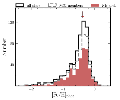
Figure 6: Photometric metallicity ([Fe/H]_phot) distribution functions (MDFs) for all stars in the NE shelf fields (including MW contaminants; black solid open histogram), stars classified as M31 members (grey dashed open histogram; Section 3.1), and stars that probably belong to the NE shelf ($p_{\rm sub}>0.5$; Section 3.2.2). We assumed 12 Gyr PARSEC isochrones (Marigo et al., 2017) to determine [Fe/H]_phot (Section 2.2). The median [Fe/H]_phot for each sample is shown as arrows, where [Fe/H]_phot,med = $-0.41$ is robust with respect to sample selection, indicating that the NE shelf is the dominant feature in the data (Section 3.3).

Table 3: Photometric Metallicity Distribution Properties for Kinematically Cold Components in the NE Shelf Fields

Comp.	$\mu_{\rm KCC}$
	[Fe/H]med	$\langle$[Fe/H]$\rangle$	$\sigma_{\rm[Fe/H]}$
Halo	…	$-0.43^{+0.01}_{-0.02}$	$-0.56$ $\pm$ 0.02	0.39 $\pm$ 0.02
NE3
KCC1	$-224.3$	$-0.51^{+0.06}_{-0.04}$	$-0.61$ $\pm$ 0.04	0.42 $\pm$ 0.03
KCC2	$-123.7$	$-0.57^{+0.01}_{-0.02}$	$-0.65$ $\pm$ 0.04	0.42${}^{+0.04}_{-0.03}$
NE1
KCC1	$-383.7$	$-0.39^{+0.00}_{-0.08}$	$-0.53^{+0.03}_{-0.04}$	0.37 $\pm$ 0.04
KCC2	$-204.2$	$-0.40^{+0.03}_{-0.02}$	$-0.49$ $\pm$ 0.03	0.37 $\pm$ 0.04
NE6
KCC1	$-398.6$	$-0.41^{+0.0}_{-0.02}$	$-0.50$ $\pm$ 0.02	0.27 $\pm$ 0.02
KCC2	$-200.9$	$-0.40^{+0.03}_{-0.02}$	$-0.49$ $\pm$ 0.03	0.34 $\pm$ 0.02
NE2
KCC1	$-310.5$	$-$0.45${}^{+0.03}_{-0.04}$	$-0.52$ $\pm$ 0.04	0.35 $\pm$ 0.05
NE4
KCC1	$-300.6$	$-0.35^{+0.02}_{-0.05}$	$-0.52$ $\pm$ 0.05	0.44 $\pm$ 0.05

• Note. — The columns are kinematical component, mean velocity (Table 3.2.2), median [Fe/H]_phot, mean [Fe/H]_phot, and standard deviation on [Fe/H]_phot. We calculated each quantity via bootstrap resampling weighted by the probability that a star belongs to a given kinematical component (Section 3.2.2). The quantities for the halo-like population across all fields are calculated analogously using $p_{\rm halo}=1-p_{\rm sub}$.

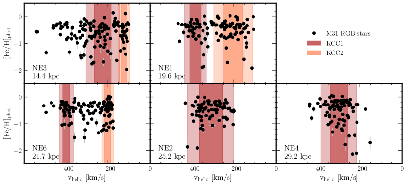
Figure 7: Heliocentric velocity ($v_{\rm helio}$) versus photometric metallicity ([Fe/H]_phot) for M31 RGB stars (black points) in the NE shelf fields, where projected M31-centric radius (R_proj) increases from left to right and top to bottom. We show the 1$\sigma$ (2$\sigma$) radial velocity range of KCC1 (red) and KCC2 (orange) (Table 3.2.2; Figure 5) as dark (light) shaded regions. The [Fe/H]_phot distributions across the various NE shelf substructure components are similar. Stars assigned to the stellar halo component also have similar [Fe/H]_phot to the NE shelf.

We investigated the photometric metallicity distribution functions (MDFs) of RGB stars along the line-of-sight to the NE shelf to probe its chemical composition. We used photometric metallicities instead of spectroscopic calcium-triplet based metallicities (e.g., Figure 4) because they are more robust at the low S/N characteristic of spectra in M31: [Fe/H]_CaT measurements are subject to larger random uncertainties than [Fe/H]_phot measurements and are unavailable for a non-negligible number of stars. Moreover, we are concerned with relative metallicity differences between NE shelf stars and other stellar populations, as opposed to absolute metallicities. We determined [Fe/H]_phot assuming 12 Gyr PARSEC isochrones (Marigo et al., 2017) following Section 2.2.

In Figure 6, we show the photometric MDFs for all stars in the NE shelf fields (including MW contaminants), stars classified as M31 members (Section 3.1), and stars that probably belong to the NE shelf ($p_{\rm sub}>0.5$; Section 3.2.2). The unweighted median (mean) [Fe/H]_phot for each sample is $-0.43$ ($-0.54$), $-0.42$ ($-0.54$), and $-0.41$ ($-0.53$), respectively. If we instead assume 10 Gyr or 8 Gyr isochrones, which approximately correspond to the mean stellar age of M31’s phase-mixed stellar halo (Brown et al., 2006, 2007, 2008) and the GSS (Brown et al., 2006; Tanaka et al., 2010), we obtain a median (mean) [Fe/H]_phot for the NE shelf that is $0.03$ ($0.04$) dex or $0.08$ ($0.09$) dex more metal-rich. The relative invariance of the median (mean) [Fe/H]_phot value with respect to the sample selection indicates that NE shelf tidal debris is the dominant feature in the data. That is, the majority of stars with successful velocity measurements are indeed M31 RGB stars (Section 3.1), although the value of [Fe/H]_phot is not physically meaningful for MW foreground stars, and the majority of RGB stars indeed belong to the NE shelf and not the phase-mixed stellar halo.

In addition, the general shape of the MDF remains relatively constant between each sample, where the MDF is skewed toward the peak at [Fe/H]_phot $\sim-0.4$, followed by a sharp decline for [Fe/H]_phot $\gtrsim-0.2$ and an extended low-metallicity tail. The fact that the metal-poor ([Fe/H]_phot $\lesssim-1.3$) population declines when selecting only for NE shelf stars ($p_{\rm sub}>0.5$; Figure 6) suggests that the majority of these stars belong to M31’s stellar halo rather than the shelf. Adopting stricter threshold for NE shelf membership ($p_{\rm sub}>0.75$) does not significantly alter the location or shape of the MDF, so we retain the more inclusive criterion to maximize the sample size of NE shelf stars.

The most pronounced change in the MDFs in Figure 6 is that a distinct peak at [Fe/H]_phot $\sim$ $-0.7$ emerges in the NE shelf sample. This feature is robust because the bin sizes (0.1 dex) for each MDF are twice the median photometric uncertainty ($0.05$ dex). This peak may originate from our choice to designate stars that probably belong to kinematical substructure ($p_{\rm sub}>0.5$) as NE shelf stars, when in reality some of these stars could belong to other dynamically cold structures such as M31’s disk (Section 3.2.3, 4.1). Interestingly, this peak metallicity roughly corresponds to the median [Fe/H]_phot of M31’s disk edge in the Pan-chromatic Hubble Andromeda Treasury (PHAT; Dalcanton et al. 2012; Williams et al. 2014) when assuming 13 Gyr isochrones (Gregersen et al., 2015).

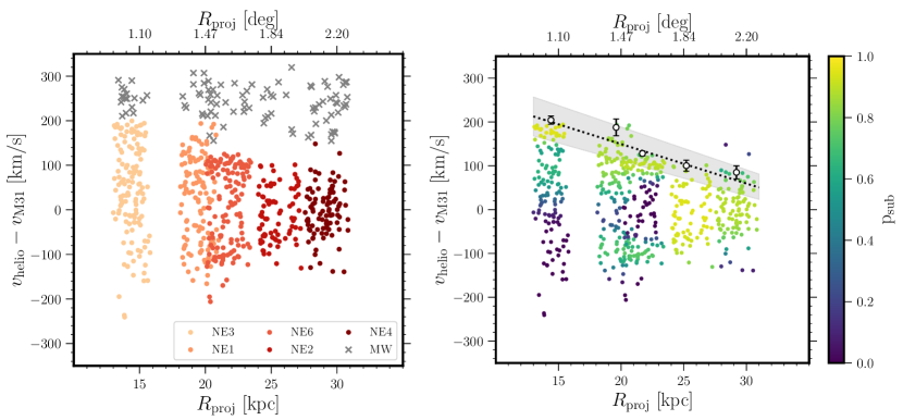
Figure 8: Heliocentric velocity relative to M31’s systemic velocity ($v_{\rm M31}$ = $-300$ km s^-1) versus projected M31-centric radius in the NE shelf fields for (left) stars with successful radial velocity measurements, including both M31 RGB stars (colored points) and MW foreground stars (grey crosses; Section 3.1), and (right) solely M31 RGB stars color-coded by their kinematically-based probability of belonging to substructure (Section 3.2.2). Velocity errors associated with individual data points are not shown for the sake of clarity (median 5.3 km s^-1). The “wedge” pattern visible in this space for M31 RGB stars is characteristic of a tidal shell formed in a radial merger (Section 3.4.1). The right panel also shows the observed upper envelope of the wedge (white open circles; Eq. 4) and its best-fit model (black dotted line, with 1$\sigma$ confidence interval as gray shaded region; Merrifield & Kuijken 1998) used to place constraints on M31’s gravitational potential (Section 3.4.2).

We further explored the [Fe/H]_phot distribution of the NE shelf by considering the relationship to radial velocity and projected M31-centric radius. Figure 7 shows $v_{\rm helio}$ versus [Fe/H]_phot for each NE shelf field ordered as a function of R_proj, where we highlighted the 2$\sigma$ radial velocity range associated with each detected kinematical substructure component (Table 3.2.2; Figure 5). We calculated the average metallicity and metallicity dispersion for each KCC weighted by the the kinematically-based probability of belonging to the given KCC (Table 3.3). We note that the metallicity difference between kinematical components is likely larger than indicated by Table 3.3 because of the probabilistic nature of the component assignment. We found that the median [Fe/H]_phot in NE3 is $\sim$0.15 dex more metal-poor than the relatively uniform metallicity of the other fields, possibly due to its more dominant halo-like population and/or larger disk contribution. The halo-like population across all fields is similar in metallicity to the combined NE shelf population. This raises the possibility that this kinematically hot component may correspond to tidal debris with a high velocity dispersion, or similarly that the stellar halo in this region is heavily polluted by NE shelf substructure. We compare the metallicity distribution of the NE shelf to M31’s phase-mixed stellar halo in Section 5.2.

Moreover, Figure 7 demonstrates that the aforementioned stars with [Fe/H]_phot $\sim$ $-0.7$ dex are visible in the secondary KCC of NE1 and possibly the primary KCC of NE3. These stars therefore have metallicities and velocities (Section 3.2.3) broadly consistent with M31’s disk, implying that a low level of disk contamination may be present in the data. However, the [Fe/H]_phot distribution for stars that probably belong to KCCs (i.e., either the NE shelf or the disk) still appears to be dominated by the NE shelf, where removing stars with $-0.65<$ [Fe/H]_phot $<-0.85$ increases the median (mean) [Fe/H]_phot by merely 0.04 (0.04) dex. The clump of stars at [Fe/H]_phot $\lesssim$ $-1.0$ in the secondary KCC of NE6 could also be associated with the disk, where removing this grouping increases the median (mean) [Fe/H]_phot by an additional 0.02 (0.04) dex.

3.4 Projected Phase Space Distribution

Prior studies (e.g., Fardal et al. 2007, 2013; Sadoun et al. 2014; Miki et al. 2016; Kirihara et al. 2017) have proposed that the NE shelf may have formed from a radial merger – a merger with low angular momentum that consequently produces shell-like tidal structures (Hernquist & Quinn, 1988; Merrifield & Kuijken, 1998; Sanderson & Helmi, 2013). These tidal structures create a “caustic surface” when viewed in radial ($r,v_{r}$) phase space, where this surface contains material with similar orbital energy that originates from the progenitor disrupted by the radial merger. Owing to the near-symmetry of this type of event, the resulting signature in projected ($R,v_{\rm los}$) phase space near the spatial edge of the shell depends only on the enclosed mass of the host galaxy and the shell radius (Merrifield & Kuijken, 1998; Ebrová et al., 2012; Sanderson & Helmi, 2013). In this section, we provide an overview of the observed features of the projected phase space distribution for the NE shelf (Section 3.4.1) before using the observed distribution to assess the ability of analytical models to constrain M31’s gravitational potential at the shelf location (Section 3.4.2).

3.4.1 Observed Features of the NE Shelf

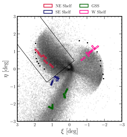
Figure 9: Histogram of the spatial distribution of satellite debris in from the F07 GSS formation model in M31-centric coordinates (Section 4). We show the spectroscopic field locations (colored rectangles) and photometric NE and W shelf edges (black points) from Figure 1. The black outlined box is the broad selection region used to initially define the simulated NE shelf.

Figure 8 shows the line-of-sight velocity ($v_{\rm helio}$) of stars in the NE shelf fields, shifted according to M31’s systemic velocity ($v_{\rm M31}=-300$ km s^-1), versus projected M31-centric radius (R_proj). In this space, M31 RGB stars clearly show a “wedge” pattern characteristic of a shell formed in a radial merger: the $v_{\rm helio}$ range decreases with increasing R_proj as stars in the shell approach apocenter, where $v_{\rm helio}$ $-$ $v_{\rm M31}\sim 0$ km s^-1. Given that the velocity dispersion of the NE shelf in the outermost field (NE4; R_proj $\sim$ 29 kpc) is relatively large ($\sigma_{v}\sim 43$ km s^-1 ; Table 3.2.2), the data may not capture the full radial extent of the shell feature (see Figure 10).

The magnitude difference between red clump stars in the NE shelf and GSS indicates that it is located in front of the latter feature given their similar CMD morphologies (Ferguson et al., 2005; Richardson et al., 2008) and consequently that the NE shelf is located in front of M31 when combined with line-of-sight distance measurements (McConnachie et al., 2003). Thus, the upper envelope ($v_{\rm helio}$$-$ $v_{\rm M31}>0$ km s^-1) of the caustic corresponds to tidally stripped stars moving toward M31, whereas the lower envelope corresponds to stars moving away from M31. In the field with the innermost robust detection of both envelopes of the wedge (NE1; Figure 5), the positive (negative) envelope has $v_{\rm helio}$ $-$ $v_{\rm M31}$ $\sim+95.8^{+11.9}_{-10.5}$ ($-83.7^{+11.2}_{-10.2}$) km s^-1 (Table 3.2.2), indicating that the wedge shape is roughly symmetric. That is, the inbound stars are moving at approximately the same speed as the outbound stars.

In addition, the right panel of Figure 8 highlights M31 RGB stars that probably belong to kinematical substructure (Section 3.2.2) dominated by the NE shelf (Section 3.3). The upper envelope appears to have a higher density of stars than the lower envelope (see also Figure 5), where the lower envelope only becomes statistically distinguishable from the background kinematically hot population at R_proj $\sim$ 19 kpc in NE1. However, the clustering of stars close to the expected velocity of the lower envelope in NE3 ($v_{\rm helio}$ $\lesssim$ $-400$ km s^-1; Figure 5) that have [Fe/H]_phot consistent with the NE shelf (Figure 7) implies that the lower envelope may be present at low levels in the data.

3.4.2 Constraints on the Gravitational Potential of M31

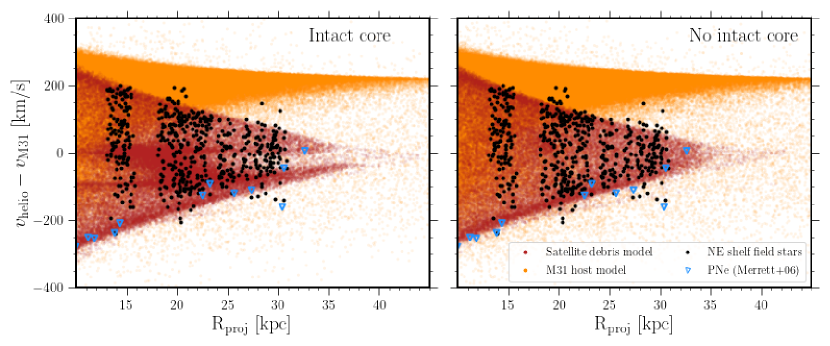
Figure 10: Similar to Figure 8, except comparing the predictions of N-body models (Fardal et al., 2007, 2012) in the NE shelf region for the formation of the GSS to observations of RGB stars (black points; this work) and PNe (blue open triangles; Merrett et al. 2003, 2006). The models contain a combined bulge, disk, and halo component for the host (orange points) and a satellite component corresponding to GSS-related tidal debris (red points). We show models for a merger remnant with (left panel) and without (right panel) an intact core. The NE shelf region is defined using $X_{\rm M31}>$ 0.2^∘ and $-1.5^{\circ}<Y_{\rm M31}<0.5^{\circ}$, where $X_{\rm M31}$ and $Y_{\rm M31}$ are defined along the NE major axis (P.A. = 38^∘ E of N) and NW minor axis, respectively. The observed projected phase space distribution of the NE shelf broadly agrees with that of a tidal shell formed from a radial merger with the GSS progenitor, where the model with a completely disrupted progenitor provides a better match (Section 4.2).

As first shown by Merrifield & Kuijken (1998), hereafter MK98, the observed line-of-sight velocities of stars in a tidal shell could in principle constrain the radial component of the gravitational potential ($g_{s}$) of the host galaxy at the shell radius ($r_{s}$). Thus, we utilized our measurements of M31-centric line-of-sight velocity ($v_{\rm los}$) for RGB stars in the NE shelf region as a test of such analytical models. The absolute maximum velocity of the wedge as a function of projected galactocentric radius $R$ is given by the following expression,

$$v_{\rm los}^{\rm MK}=\sqrt{\frac{g_{s}}{r_{s}}}(r_{s}-R).$$ (2)

MK98 derived Eq. 2 assuming that a tidal shell is composed of stars on monoenergetic orbits in a plane tangential to the line of sight, where stars in the shell have low angular momentum such that the three-dimensional shell velocity ($v_{s}$) is zero. We adopted Eq. 2 to describe the shape of the NE shelf wedge pattern instead of the formulation by Sanderson & Helmi (2013), hereafter SH13,

$$v_{\rm los}^{\rm SH}=\frac{\sqrt{r_{s}^{2}+2Rr_{s}-3R^{2}}(\sqrt{g(r_{s})(r_{s}-R)}+v_{s})}{r_{s}+R},$$ (3)

which lifts the monoenergetic and low angular momentum assumptions, because the simpler MK model exhibits better convergence when applied to the data. The reason for this is likely that the tip of the wedge pattern, which places the strongest constraints on $v_{s}$, is not included in the NE shelf data (Section 3.4.1), in conjunction with the fact that $v_{s}$ is instrinsically difficult to constrain with typical values of $\lesssim$ 30 km s^-1 (SH13).

In order to estimate $g_{s}$, we therefore fit Eq. 2 to the upper envelope of the NE shelf wedge pattern. We used the upper, as opposed to the lower, envelope owing to projection effects (SH13) that result in a minor asymmetry in which the positive edge has a greater maximum apparent speed for the innermost field (Figure 8), besides which the detection of the lower envelope in this field is uncertain (Section 3.4.1). We used the kinematical parameters from Table 3.2.2 to define the upper envelope using the following equation for each NE shelf field

$$v_{\rm los}=\mu_{v,{\rm KCC2}}+2\sigma_{v,{\rm KCC2}}-v_{\rm M31},$$ (4)

where we calculated $\delta v_{\rm los}$ using standard error propagation by assuming symmetric average uncertainties on $\mu_{v,{\rm KCC2}}$ and $\sigma_{v,{\rm KCC2}}$. We assessed the possibility of disk contamination in KCC2 of NE1 by conservatively removing all stars with [Fe/H]_phot in the range expected for the majority of disk stars (Section 3.3) and found that the upper envelope location was unchanged.

Thus, we used the non-linear least squares Python algorithm curve_fit (Virtanen et al., 2020) to obtain $g_{s}=$ 3.04 $\pm$ 0.80 km s^-1 Myr^-1 and $r_{s}=$ 36.6 $\pm$ 2.7 kpc from the observed shape of the NE shelf wedge. The right panel of Figure 8 shows the data points corresponding to the upper edge of the feature and its best-fit model. Assuming a spherical potential, we can transform these constraints into an upper limit on M31’s enclosed mass ($M_{\rm enc}$) at the shell radius,

$$M_{\rm enc}(r<r_{s})=\frac{g_{s}r_{s}^{2}}{G},$$ (5)

where we found that $M_{\rm enc}$($r<$ 36.6 kpc) = (9.26 $\pm$ 2.78) $\times$ 10¹¹ $M_{\odot}$ based on the NE shelf data.

We note that these parameter estimates should be treated with caution given the assumptions involved in the derivation of Eq. 2. SH13 used the Fardal et al. (2007) GSS merger simulations to compare the value of $g_{s}$ derived from the projected phase space distributions of predicted caustics to the true values in the simulation. They found that the MK model overestimated the value of $g_{s}$ by a factor of $\sim$2-3, whereas the more sophisticated SH13 model produced more accurate estimates. Thus, the empirically derived value of $g_{s}$ should be interpreted as an upper limit. We compare this value to literature measurements of M31’s enclosed mass in Section 6.1.

4 N-body Models for the Formation of the Northeast shelf

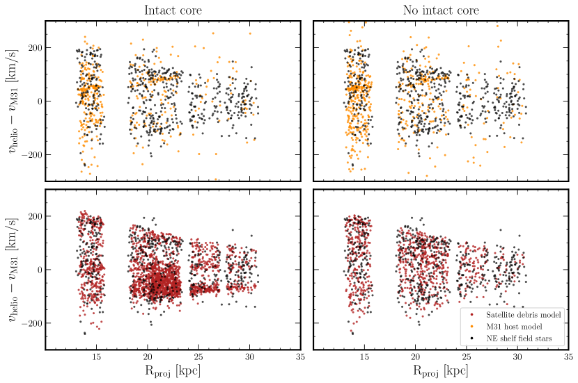
Figure 11: Similar to Figure 10, except we restricted the selection region for the NE Shelf in the N-body models to the location of the spectroscopic fields (Figure 1). Top panels (bottom panels) show the comparison to the M31 host (satellite debris) models with (left panels) and without (right panels) an intact core. The NE shelf region in the simulations is dominated by tidal debris, as opposed to the disk or phase-mixed stellar halo, at the data location, although the models predict a non-negligible disk contribution from $v_{\rm helio}-v_{\rm M31}\sim+(50-150)$ km s^-1 at R_proj $\lesssim$ 23 kpc (Section 4.1).

We compared observations of RGB stars in the NE shelf to predictions of N-body models for the GSS merger event to test scenarios for the shelf’s formation. We utilized re-simulations of models from Fardal et al. (2007), hereafter F07, and Fardal et al. (2012), hereafter F12, which were constructed using a static bulge–disc–halo model for M31’s gravitational potential (Geehan et al., 2006) and a spherical Plummer model for a satellite progenitor consisting of only a stellar component (Fardal et al., 2006). A particle realization for the M31 host component was incorporated following the conclusion of the dynamical evolution of the N-body satellite model. In the F07 (F12) model, complete (partial) disruption of a satellite with stellar mass $M_{s}=2.2\times 10^{9}\ M_{\odot}$ ($3.1\times 10^{9}\ M_{\odot}$) occurs 0.84 Gyr (0.97 Gyr) ago within a M31 host with stellar mass $M_{h}=1.1\times 10^{11}\ M_{\odot}$ and virial mass $M_{200}=1.7\times 10^{12}\ M_{\odot}$ for each simulation.

For the F07 and F12 models, respectively, the orbit of the progenitor was fitted to reproduce the observed properties of the GSS, not those of the NE, W, or SE shelves. Despite this, the models have shown good agreement with kinematics of RGB stars in the SE and W shelves (Gilbert et al., 2007; Fardal et al., 2012) and promising overlap with PNe kinematics for a small sample in the NE shelf region (Merrett et al., 2003, 2006; Fardal et al., 2007, 2013). Figure 9 shows the satellite debris distribution on the sky for the F07 model, where the distribution for the F12 model is similar.

4.1 Predicted Projected Phase Space Distributions

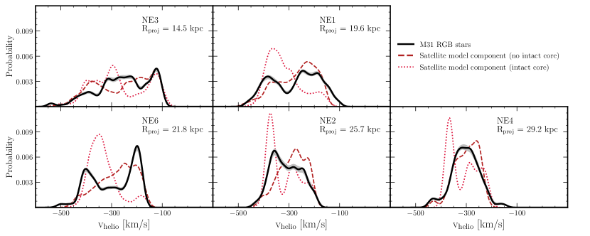
Figure 12: Line-of-sight velocity distributions predicted for the NE shelf at the field locations (Figure 11) by N-body models for the formation of the GSS (Fardal et al., 2007, 2012) compared to observations of M31 RGB stars in the NE shelf (cf. Figure 5). We represent the velocity distributions using Gaussian kernel density estimation with $\sigma$ = 15 km s^-1. We show the predicted velocity distributions for the satellite debris components of the models with (red dotted lines) and without (red dashed lines) an intact core over the radial range spanned by each spectroscopic field. We also show the 1$\sigma$ confidence intervals (grey shaded regions) from the velocity measurement uncertainty on the observed distributions (solid black lines). Neither model is able to reproduce the velocity distributions in detail, although the model without an intact core is a better match (Section 4.2).

To assess whether this agreement extends to the kinematics of RGB stars in the NE shelf over a larger spatial extent, we compared the predicted projected phase space distributions to the observations in Figure 10. We also show the PNe observations from Merrett et al. (2003, 2006) identified as a possible continuation of the GSS. We initially selected the NE shelf region in the simulations using the criteria $X_{\rm M31}>$ 0.2^∘ and $-1.5^{\circ}<Y_{\rm M31}<0.5^{\circ}$ (Figure 9), where $X_{\rm M31}$ and $Y_{\rm M31}$ are defined along the NE major axis (P.A. = 38^∘ E of N) and NW minor axis in the tangent plane. We first chose to inspect the NE shelf over a larger spatial area than spanned by the spectroscopic fields for better statistical representations of the models. Additionally, we separated the N-body model particles into M31 host and GSS-related satellite debris components in Figure 10.

For models with (F12) and without (F07) an intact satellite progenitor core, the projected phase space distribution of the tidal debris clearly provides a qualitative match to the NE shelf data. This not only supports the empirically motivated conclusion that the NE shelf is indeed a tidal shell (Section 3.4.1), but also provides compelling evidence in favor of a GSS-related origin. For the first time, we present a complete detection of the characteristic wedge pattern in the sense that it includes the returning stream component (i.e., the positive-velocity upper envelope) of the NE shelf. However, Figure 10 supports the notion that the NE shelf observations do not resolve the tip of the wedge pattern (Section 3.4.1) predicted to reside at R_proj $\gtrsim$ 35 kpc, where the tip is required to provide constraints on the 3D shell velocity (Section 3.4.2). Figure 10 also corroborates the fact that the predicted negative-velocity caustic at R${}_{\rm proj}\sim$ 15 kpc does not appear to be detected in the data (Section 3.2). In general, the modeled upper envelopes of the wedge pattern appear to provide better fits to the data than the lower envelopes.

In order to explore predictions more equivalent to the observations, we restricted the NE shelf selection region in the models to an area similar to the spatial coverage of the spectroscopic fields in Figure 11. We found that the modeled disk contribution is substantially lower at the location of the NE shelf fields (in contrast to the broad selection region used in Figure 10). In the model with (without) an intact core, the host component constitutes 16.3% (41.1%) of the total particles, indicating that the expected satellite debris density is higher for the intact core model (Section 4.2). The M31 host model predicts a non-negligible disk component at $v_{\rm helio}-\ v_{\rm M31}\sim+30$, $+55$, and $+70$ km s^-1 that overlaps with the primary, secondary, and secondary KCCs in NE3, NE1, and NE6, respectively, all of which are suspected of being contaminated by the disk (Section 3.2.3, Section 3.3). The contamination from the host decreases with projected radius, where the specific fractional contributions depend on the satellite model assumptions. Furthermore, the relative fraction of host versus satellite debris material is highly dependent on model assumptions regarding M31’s mass and structural components.

4.2 Remnant Core or Complete Disruption of the Satellite Progenitor?

We evaluated whether the model with (F12) or without (F07) an intact satellite progenitor core provides a better fit to the observations. Figures 10 and 11 show that the primary difference between the projected phase space distributions of models with and without an intact core is a relative enhancement of structure (cf. Fardal et al. 2013) at $v_{\rm helio}-\ v_{\rm M31}\lesssim 0$ km s^-1 and an associated dearth of material approaching the tip of the wedge pattern. From an initial inspection, the model without an intact core appears to provide a better match to the data, given the lack of obvious clumping in the interior of the observed wedge pattern (excepting perhaps the third component of unclear origin in NE3; Section 3.2).

We further demonstrate the incompatibility of the intact core model in Figure 12, where we show the predicted versus observed line-of-sight velocity distributions for the NE shelf. The observed distribution is constructed from all RGB stars in the NE shelf fields, given evidence that the population is dominated by tidal debris (Section 3.3). The model distributions are constructed using only the satellite debris component at the data location (used in Figure 11). In each case, we represent the velocity distributions using Gaussian kernel density estimation with $\sigma$ = 15 km s^-1. We calculated the uncertainty in the observed distribution via 10³ perturbations by the (Gaussian) velocity uncertainties and re-evaluations of the kernel-smoothed probability density functions. The predicted line-of-sight velocity distributions constructed when including the host component are qualitatively consistent with those based solely on the satellite component for the F12 model. The main change for the F07 model is the addition of a peak at $v_{\rm helio}$ $\sim$ $-270$ km s^-1 in NE3 caused by the disk.

Although Figure 12 shows that the models can roughly mimic the behavior of the observed line-of-sight velocity as a function of radius, particularly in terms of the width of the distributions, neither model provides an ideal match to the data. For example, the prominence and location of the negative-velocity edges of the modeled distributions, which correspond to the lower envelopes of the wedge patterns, do not approximate the data well. This disagreement is more pronounced for the F12 model than the F07 model. The F12 model also predicts more structure near M31’s systemic velocity for R_proj $\lesssim$ 22 kpc than is observed in the distributions.

We quantified the degree of similarity between modeled and observed velocity distributions as a function of radius using an Anderson-Darling test. We performed 10³ trials in which we computed the test statistic between the perturbed observed velocity distributions and a random sampling of equal size from the models at the data location. The null hypothesis that the F12 model with an intact core is drawn from the same underlying distribution as the data can be rejected below the $\sim$5% level in NE1, NE6, and NE4, but not below the $\sim$15% level for the other fields. The F07 model can be rejected at the $\sim$5% level for NE2 but is consistent above the 10% for all other fields. Including the host component does not alter these conclusions for either model.

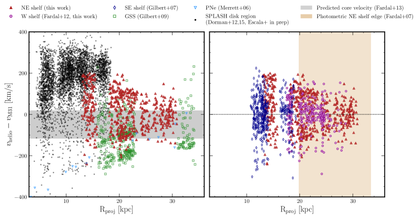
Figure 13: Heliocentric velocity relative to M31’s systemic velocity versus projected M31-centric radius for M31 RGB stars (Section 5.1) along the line-of-sight to the GSS (green open squares; Gilbert et al. 2009), the NE (red filled triangles; this work), W (outlined magenta circles; F12), and SE (blue open diamonds) shelves, and the region of M31’s northeastern disk surveyed by SPLASH (black points; Dorman et al. 2012, 2015). We also show PNe that are possibly GSS-related (blue open inverted triangles; Merrett et al. 2003, 2006). Each RGB sample contains stars belonging to the phase-mixed stellar halo in addition to substructure (i.e., the disk and/or tidal debris). (Left panel) The NE shelf compared to the GSS and the disk region. The secondary kinematical component along the GSS known as the KCC (Kalirai et al., 2006; Gilbert et al., 2009) is located at $v_{\rm helio}-v_{\rm M31}>-150$ km s^-1 and R${}_{\rm proj}<25$ kpc, overlapping with the lower envelope of the NE shelf. We do not find clear evidence for a continuation of the NE shelf in the disk region or an intact progenitor core based on its predicted velocity range (Section 4.2; Fardal et al. 2013). (Right panel) The shell patterns for the NE, W, and SE shelves, which are predicted to correspond to successive orbital wraps of GSS-related tidal debris. We show the projected radial range of the NE shelf edge inferred from imaging by F07 for reference.

In summary, the best available observational evidence favors a scenario in which the satellite progenitor that produced the NE shelf has completely disrupted, or at least is not present in the NE shelf region probed in this work, although comparison with a larger suite of N-body models is necessary for confirmation. If the intact core of the progenitor does exist, it could instead be embedded in the disk at $v_{\rm helio}-v_{\rm M31}\sim-49\pm 67$ km s^-1 compared to typical disk velocities of $v_{\rm helio}-v_{\rm M31}\sim+80\pm 40$ km s^-1 at predicted core positions (Fardal et al., 2013).In the SPLASH survey of M31’s disk, Dorman et al. (2012) tentatively detected NE shelf tidal debris as a forward continuation of the GSS at $v_{\rm helio}$ $<-500$ km s^-1, but did not find evidence of a velocity signature resembling that of an intact core. We further explore the possibility that the progenitor core is present in the SPLASH disk data in Section 5.1. We also discuss literature models for the NE shelf’s formation in the context of our observations in Section 6.2.

5 Comparison to the Disk, West and Southeast Shelves, and the Giant Stellar Stream

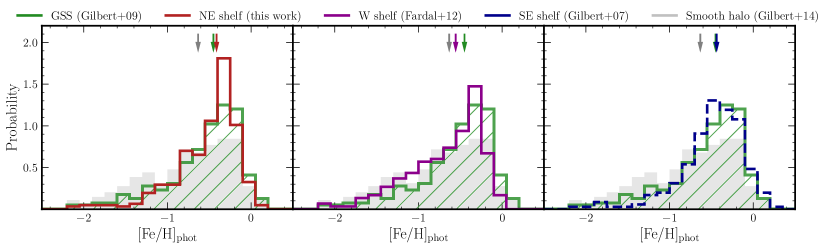
Figure 14: Photometric MDFs for the NE shelf (red histogram, left panel), W shelf (magenta histogram, middle panel), and SE shelf (blue histogram, right panel) compared to the GSS (green hatched histograms) and the smooth halo (gray filled histograms). Each stream/shelf sample consists of stars classified as M31 members (Section 3.1, 5.1) that probably belong to a given tidal feature ($p_{\rm sub}>0.5$; Section 3.2.2, 5.2). The smooth halo sample is made from M31 members in SPLASH halo fields spanning 12–33 kpc (Gilbert et al., 2012) with $p_{\rm sub}<0.2$. We determined [Fe/H]_phot for the smooth halo, GSS, W shelf, and SE shelf homogeneously with the NE shelf (Section 2.2). The median [Fe/H]_phot for each sample is shown as arrows (Table 4). The NE shelf has the same metallicity as the GSS and the SE shelf and is distinct from the smooth halo. The median [Fe/H]_phot of the W shelf MDF is lower due to contamination by metal-poor halo stars, but shares a similar MDF peak.

5.1 Projected Phase Space Distributions

We compared the projected phase space distribution of the NE shelf to the W and SE shelves and the GSS to explore the relationship between the likely associated tidal features. Figure 13 shows M31-centric heliocentric velocity versus projected M31-centric radius for the NE shelf (this work), the GSS (Gilbert et al. 2009, hereafter G09), and the W (F12) and SE (Gilbert et al. 2007, hereafter G07) shelves, in addition to the stream PNe from Merrett et al. (2003, 2006). We also compared the NE shelf to M31’s disk as surveyed by SPLASH (Dorman et al., 2012, 2015) given that the intact core of the GSS progenitor may be embedded in the disk (Section 4.2).

For each feature, we show only stars that are more likely to belong to M31 than the MW foreground. For the GSS and SE shelves, M31 membership was evaluated using the likelihood-based method of Gilbert et al. (2006) as part of the SPLASH survey of M31’s halo. In contrast to F12, we utilized the Bayesian technique by Escala et al. (2020b) to identify M31 stars (Section 3.1) in the W shelf, where this approach produces similar results to the original Gilbert et al. method. We excluded the innermost W shelf field (Figure 1) from our analysis owing to contamination by NGC 205 (F12). For stars in the SPLASH disk region, membership was determined from CMD position and the absorption strength of the Na I $\lambda$8190 doublet (I. Escala et al., in preparation). We note that we do not distinguish between RGB stars belonging to substructure (i.e., the disk and/or tidal debris) and the phase-mixed halo in Figure 13.

The right panel of Figure 13 suggests that the NE, W, and SE shelves form a sequence of tidal shells at successively lower energy. This fits with the prediction that they correspond to GSS progenitor tidal debris approaching its second, third, and fourth pericentric passage, respectively (e.g., F07, Fardal et al. 2013). The NE shelf is the outermost shell, extending to R${}_{\rm proj}\gtrsim 31$ kpc and spanning $\lesssim$ 400 km s^-1, whereas the W and SE shelves are contained within R${}_{\rm proj}\sim 25$ kpc and $\sim 18$ kpc respectively and $|v_{\rm helio}-v_{\rm M31}|\sim 100$ km s^-1. For reference, we show the projected radial range of the NE shelf edge inferred from imaging by F07, where the geometrical orientation of the shell relative to the line-of-sight causes this apparent variation in R_proj. Regardless of whether GSS formation models can match detailed observations in the shelves (Section 4), their concentric wedge patterns provide compelling evidence for a shared origin in the tidal disruption of a single satellite galaxy.

The left panel of Figure 13 shows the NE shelf compared to the GSS and the disk region. The GSS fields include a secondary kinematical component known as the KCC that is likely physically associated with the GSS based on their tight correlation in R_proj versus $v_{\rm helio}$ space (Figure 13) and chemical similarities (Kalirai et al., 2006; Gilbert et al., 2009, 2019). Additionally, the potential forward continuation of the GSS speculated to be the NE shelf by Dorman et al. (2012) (Section 4.2) is visible in the disk data at $v_{\rm helio}-v_{\rm M31}<-200$ km s^-1 and R_proj $\lesssim$ 15 kpc. However, this group of stars does not seem to be consistent with an inward extension of the lower envelope of the NE shelf wedge pattern as probed by our data. The lower envelope of the NE shelf instead overlaps in phase space with the KCC.

In a minor merger scenario for the formation of the GSS, the KCC could originate from an extension of the shelves (G09). The W shelf is the most promising candidate because its extent is not well-constrained owing to obscuration by M31’s southwestern disk. Moreover, GSS formation models predict negligible contributions from the NE and SE shelves along the GSS (F07, F12). For the KCC to originate from a symmetric extension of the NE shelf, it would minimally require that the positive velocity caustic of the shell was depopulated at the KCC location. Additional GSS formation models will be necessary to evaluate this possible origin for the KCC.

Figure 13 also shows the predicted velocity range of an intact GSS progenitor core, $v_{\rm helio}-v_{\rm M31}=-49\pm 67$ km s^-1 (Fardal et al., 2013) compared to the expanded SPLASH disk dataset (i.e., including spectroscopic fields published by Dorman et al. 2015). As in the case of the NE shelf (Section 4.2), we do not find evidence for the presence of an intact core in the SPLASH data based on current theoretical predictions. The apparent clumps of stars at R_proj $\sim$ 5–8 kpc within the predicted velocity range are probably associated with the disk, which approaches more halo-like velocities in this radial range (Dorman et al., 2012). Such clumps in velocity space also do not correspond to any spatial concentrations that would resemble a core. Moreover, the most likely locations for the core position are nearer to the NE shelf, not within the inner 5–8 kpc of the disk, although this radial range is not excluded by the models (Fardal et al., 2013). We note that Davidge (2012) identified an overdensity at R_proj $\sim 3.5$ kpc that is a plausible candidate for the GSS core, but this is outside the innermost extent of the SPLASH survey region.

5.2 Photometric Metallicity Distributions

Table 4: Photometric Metallicity Distribution Properties for the Smooth Halo, GSS and NE, W, and SE Shelves

Feature	[Fe/H]phot,med	$\langle$[Fe/H]phot$\rangle$	$\sigma_{\rm[Fe/H]_{phot}}$
Smooth Halo	$-0.63^{+0.03}_{-0.05}$	$-0.75\pm 0.03$	$0.53\pm 0.02$
GSS	$-$0.43${}^{+0.02}_{-0.03}$	$-$0.56 $\pm$ 0.02	0.45 $\pm$ 0.02
NE shelf	$-$0.42 $\pm$ 0.01	$-$0.53 $\pm$ 0.02	0.39 $\pm$ 0.02
W shelf	$-$0.55 $\pm$ 0.04	$-$0.67${}^{+0.02}_{-0.03}$	0.43 $\pm$ 0.02
SE shelf	$-$0.44${}^{+0.02}_{-0.01}$	$-$0.50 $\pm$ 0.02	0.39 $\pm$ 0.02

• Note. — Similar to Table 3.3, except comparing the NE shelf to likely associated tidal features and the smooth halo. We measured [Fe/H]_phot homogeneously for each feature following Section 2.2. References for the original data: Halo (Gilbert et al., 2014), GSS (Gilbert et al., 2009), W shelf (Fardal et al., 2012), SE shelf (Gilbert et al., 2007).

We assessed whether the [Fe/H]_phot distributions of M31’s giant stream and shell system support the prediction that each feature originates from the disruption of a single progenitor. Figure 14 shows MDFs for the NE, W, and SE shelves compared to the GSS and the phase-mixed (“smooth”) component of the stellar halo. We assembled the smooth halo sample from M31 members in SPLASH halo fields spanning 12–33 kpc (Gilbert et al., 2012, 2014). We measured [Fe/H]_phot homogeneously for each sample following Section 2.2. In order to separate tidal debris from smooth halo stars, we calculated substructure probabilities ($p_{\rm sub}$; e.g., Section 3.2.2) for all RGB stars (Section 5.1) along the line-of-sight to each sample. For the GSS, SE shelf, and smooth halo, we employed G18’s velocity distribution models to determine $p_{\rm sub}$, whereas we performed our own modeling of the velocity distribution for the W shelf (Appendix A).

We defined the tidal debris MDFs using stars that are more likely to belong to substructure than to the kinematically hot halo-like population ($p_{\rm sub}>0.5$). We adopted this more inclusive threshold for substructure membership (as opposed to $p_{\rm sub}>0.75$) to maximize the sample size for the SE shelf, where its velocity signature at the base of its wedge pattern ($v_{\rm helio}$ $\sim$ $-300$ km s^-1, $\sigma_{v}\sim 55$ km s^-1; G07, G18) makes it difficult to disentangle from the halo. The SE and W shelf MDFs are the most likely to suffer from halo contamination, where the maximum values of $p_{\rm sub}$ are $\sim$82% and $\sim$89%, respectively, whereas the GSS and NE shelf achieve maximum values of $\sim$95%. We used $p_{\rm sub}<0.2$ to conservatively define the smooth halo MDF.

Figure 14 demonstrates that the peak metallicities ([Fe/H]_phot $\sim$ $-0.40$; Table 4) and shapes of the MDFs are similar between the shelves and the GSS, whereas they are distinct from the smooth halo MDF ([Fe/H]_phot $\sim$ $-0.6$). The median (mean) [Fe/H]_phot of the W shelf is more metal-poor than the GSS and the other shelves, but this discrepancy likely results from increased contamination by comparatively metal-poor halo stars at [Fe/H]_phot $\lesssim$ $-0.7$. Based on an iterative analysis in which substructure probabilities were calculated using both chemical and kinematical information, F12 amplified differences between the tidal debris and phase-mixed halo populations in the W shelf region to show that the [Fe/H]_phot $\gtrsim$ $-0.7$ metallicity range is dominated by the W shelf. Previous analyses of the [Fe/H]_phot distributions of the W and SE shelves (F12, G07) found agreement with the GSS, supporting a common origin scenario for these tidal features. Escala et al. (2021) also found agreement between spectral-synthesis based measurements of [Fe/H] and [$\alpha$/Fe] in the SE shelf and GSS as part of the Elemental Abundances in M31 survey.

Figure 14 further shows that the metallicity distribution of the NE shelf broadly agrees with the GSS, and by extension the W and SE shelves. We tested the hypothesis that the NE shelf and GSS MDFs share a common origin using a $p_{\rm sub}$-weighted Anderson-Darling test with 10³ bootstrap resamplings, finding that it could not be rejected below a 5% significance level. This conclusion is not affected by the selection criterion for NE shelf and GSS stars (i.e., by halo contamination) given that these regions are heavily polluted by tidal debris (Section 3.3; G09). Thus, the chemical similarity between the NE shelf and the GSS/other shelves provides evidence in favor of a direct physical association between the tidal features, especially given the independent corroboration by the projected phase space distributions (Section 5.1).

6 Discussion

6.1 The Enclosed Mass of M31

We compared the estimate of M31’s enclosed mass from NE shell kinematics (Section 3.4.2), $M_{\rm enc}=$ (9.26 $\pm$ 2.78) $\times 10^{11}M_{\rm\odot}$ at a shell radius $r_{\rm s}$ = 36.6 $\pm$ 2.7 kpc, to recent literature measurements of M31’s virial mass (see e.g., Evans & Wilkinson 2000 and Klypin et al. 2002 for earlier measurements) from various kinematic tracers. From M31’s satellite galaxies, Watkins et al. 2010, Tollerud et al. (2012), and Patel et al. (2017) measured consistent virial masses in the 1$\sigma$ range of $M_{\rm 200}=$ (1.0—1.8) $\times 10^{12}M_{\rm\odot}$. An analysis using globular cluster kinematics by Veljanoski et al. (2013) found agreement with values of $M_{\rm 200}=(1.0-1.7)\times 10^{12}M_{\rm\odot}$. Additionally, applying the timing argument to measure the masses of the MW and M31 simultaneously yields $M_{\rm 200,M31}=(1.5\pm 0.4)\times 10^{12}M_{\rm\odot}$ when combined with previous observational estimates of M31’s virial mass (van der Marel & Guhathakurta, 2008; van der Marel et al., 2012). The Bayesian sampling approach of Fardal et al. (2013) to infer M31’s virial mass from GSS merger models is also in accord with other measurements, where they found $\log_{\rm 10}(M_{\rm 200}/M_{\rm\odot})=$ 12.23 $\pm$ 0.10.

Owing to the general agreement between measurements of M31’s virial mass and the fact that Fardal et al. (2013) similarly used tidal debris to obtain their measurement, we focused on comparisons to their analysis to place our mass estimate in context. We converted Fardal et al.’s value into an estimate of the enclosed halo mass at the NE shell radius according to their assumed Navarro-Frenk-White (NFW) profile, finding $M_{\rm enc,halo}(r=r_{s})=$ (3.48 $\pm$ 0.49) $\times 10^{11}M_{\rm\odot}$. To obtain the total enclosed mass including baryons, we incorporated the mass of the bulge associated with the NFW profile ($M_{\rm b}=3.40\times 10^{10}M_{\rm\odot}$) and the mass of the disk at the NE shell radius projected onto the disk plane. Given the total mass of the disk in the simulations ($M_{\rm d,tot}=7.34\times 10^{10}M_{\rm\odot}$), its scale length ($R_{\rm d}=5.40$ kpc), and assuming $R_{s}$ = 40 kpc (the maximum value of R_disk in the field at the tip of the wedge pattern, NE4), $M_{\rm d}(r=r_{s})=$ 7.29 $\times 10^{10}M_{\odot}$. The enclosed mass at the NE shell radius deduced from Fardal et al. 2013 is therefore $M_{\rm enc}(r=r_{s})=$ (4.55 $\pm$ 0.49) $\times 10^{11}M_{\rm\odot}$.

This calculation validates the interpretation of the MK-based approximation (Eq. 2) of the enclosed mass as a likely overestimate (Section 3.4.2; F07, SH13) by a factor of 2.04 $\pm$ 2.82. Future work could simultaneously leverage measurements from the NE, W, and SE shelves—either in combination with N-body models or more sophisticated numerical implementations of the shell equations—to improve constraints on M31’s enclosed mass from shell kinematics.

6.2 Implications for GSS Merger Scenarios

We discuss the implications of the projected phase space and metallicity distributions of the NE shelf for aspects of GSS merger scenarios not considered in Sections 4 and 5. As previously established, the NE shelf metallicity distribution can place unique constraints on GSS formation models that track metallicity because the metal-rich central debris of the progenitor most likely pollutes this region (Fardal et al., 2008; Miki et al., 2016; Kirihara et al., 2017). For example, Miki et al. (2016) predicted that an observed negative metallicity gradient in the GSS (Ibata et al., 2007; Gilbert et al., 2009; Conn et al., 2016; Cohen et al., 2018; Escala et al., 2021) should result in higher metallicity for the NE shelf than other GSS-related tidal structures, whereas the W shelf and GSS metallicity should be comparable (as found by F12). In contrast, the NE shelf metallicity distribution appears to be consistent with that of the W shelf and GSS (Section 5.2) rather than being more metal-rich. However, more detailed explorations of the NE shelf MDF (Section 3.3) may reveal subtle variations on the sky that could be mapped to model predictions.

Regarding the projected phase space distribution of the NE shelf, Fardal et al. (2013) found that N-body models with high values of satellite progenitor mass and central density corresponded to the presence of a large intact core in the NE shelf region. The lack of an apparent core in the NE shelf (Section 4.2) or the neighboring disk (Section 5.1) therefore supports a lower central density and mass for the progenitor such that it completely disrupts in the case of a minor merger. In a major merger, the progenitor core has been suggested to be fully disrupted (Hammer et al., 2018) or intact in the form of M32 (D’Souza & Bell, 2018), although this latter possibility is in direct contradiction to the positions and velocities of central orbits consistent with the shelves in the Fardal et al. models.

Both minor and major merger models have found that observational constraints from the GSS (and the disk for major mergers) allow for more variation in the NE shelf location than other shelves (Fardal et al., 2013; Hammer et al., 2018). In the Hammer et al. simulations, the NE shelf often appears smaller on the sky than observed, highlighting the need for major merger models to explore whether they can reproduce M31’s shell system in detail. In any given scenario, the impact of significant internal rotation in the progenitor on the distribution of tidal debris in the shelves similarly warrants further examination (e.g., Fardal et al. 2008; Kirihara et al. 2017; D’Souza & Bell 2018), where in this work we have only performed comparisons to models with spheroidal progenitors (Section 4). Thus, the combination of new observational constraints for the NE shelf presented in this work and existing constraints from prior studies of the W and SE shelves (G07, F12) have great potential for refining future GSS merger models.

7 Summary

We have measured radial velocities and photometric metallicities from Keck/DEIMOS spectra of 556 RGB stars spanning 13—31 projected kpc along the line-of-sight to M31’s NE shelf. We have performed the first detailed kinematical and chemical characterization of RGB stars in the NE shelf and have presented the first complete detection of a “wedge” pattern in projected phase space (i.e., that includes the returning stream component of the shelf; Section 3.4.1). This study presents conclusive evidence that (1) the NE shelf is indeed a tidal shell as inferred from prior studies and (2) the NE shelf forms a multiple shell system together with the W and SE shelves (Section 5.1). We have also found that:

1. The photometric MDF of RGB stars along the line-of-sight to the NE shelf (median [Fe/H]_phot = $-0.42$ $\pm$ 0.01) is likely dominated by tidal debris as opposed to M31’s disk or phase-mixed component of M31’s stellar halo, although there is evidence for a low level of disk contamination (Section 3.3).

2. The MDF of the NE shelf is consistent with the GSS and W and SE shelves, supporting a direct physical association between the tidal features (Section 5.2).

3. The projected phase space distribution of the NE shelf exhibits broad agreement with GSS formation models in which the NE shelf is the second orbital wrap of the progenitor (F07, F12; Section 4.1), thereby providing support for this origin in a minor merger scenario.

4. There is currently no evidence for a kinematical signature in the NE shelf region (Section 4.2) or in the neighboring disk (Section 5.1) corresponding to an intact GSS progenitor core, thereby favoring formation models in which the progenitor is completely disrupted (Section 6.2).

5. Regardless of the degree to which the model predictions and observations of the NE shelf agree (Section 4), the simplicity of a common origin scenario for explaining the concentric wedge patterns of the NE, W, and SE shelves independently provides proof in its favor (Section 5.1).

6. The projected phase space distribution of the NE shelf in combination with analytical models for tidal shell formation constrains M31’s enclosed mass to an upper limit of (9.26 $\pm$ 2.78) $\times$ $10^{11}M_{\odot}$ at a shell radius of 36.6 $\pm$ 2.7 kpc (Section 3.4.2), which is likely an overestimate by approximately a factor of two in agreement with expectations from simulations (Section 6.1).

Appendix A Empirical Modeling of the W Shelf Velocity Distribution

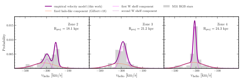
Figure 15: Same as Figure 5, except for the W shelf. We excluded the innermost spectroscopic field targeting the W shelf (Figure 1) from the analysis in Section 5 owing to contamination from NGC 205 (F12). We separated the W shelf fields into radial zones similar to those utilized by F12 for the velocity distribution modeling (Section 3.2).

Table 5: Empirical Velocity Distribution Model Parameters for the W Shelf

Field	Rproj
	$\mu_{\rm halo}$
	$\sigma_{\rm halo}$
	$\mu_{\rm KCC1}$
	$\sigma_{\rm KCC1}$
	$f_{\rm KCC1}$
	$\mu_{\rm KCC2}$
	$\sigma_{\rm KCC2}$
	$f_{\rm KCC2}$
	(km/s)
Zone 2	18.1	$-$324.8	98.1	$-$295.5${}^{+26.8}_{-16.9}$	24.4${}^{+14.0}_{-9.4}$	0.20${}^{+0.13}_{-0.10}$	$-$213.6${}^{+4.9}_{-5.4}$	16.3${}^{+5.1}_{-3.8}$	0.33${}^{+0.09}_{-0.09}$
Zone 3	21.2	$-$325.3	98.1	$-$282.9${}^{+4.9}_{-4.7}$	30.0${}^{+4.5}_{-4.0}$	0.58${}^{+0.08}_{-0.08}$	…	…	…
Zone 4	24.3	$-$323.3	98.0	$-$312.2${}^{+2.4}_{-2.4}$	13.3${}^{+2.7}_{-2.1}$	0.48${}^{+0.07}_{-0.07}$	…	…	…

• Note. — Same as Table 3.2.2, except for the W shelf.

In Section 5.2, we compared the photometric MDFs of the NE shelf to those of the GSS, SE shelf, and W shelf. This comparison requires the identification of RGB stars that probably belong to substructure in order to select a relatively clean sample of stars associated with the various tidal debris features. Although the observed velocity distributions of the GSS and SE shelf have been previously modeled empirically (Gilbert et al., 2018) similar to the NE shelf (Section 3.2), this is not the case for the W shelf. In order to calculate a MDF for the W shelf, F12 instead used their N-body model for the GSS merger to evaluate the likelihood that a RGB star belonged to GSS tidal debris versus their M31 host model constructed from a disk and halo component (Section 4). Thus, we empirically modeled the velocity distribution of the W shelf using a Gaussian mixture following Section 3.2.

We separated the W shelf fields into radial zones analogous to those used by F12, where we discarded the innermost field (F12’s Zone 1) from the analysis owing to contamination from NGC 205. We incorporated the outermost field (F12’s Zone 5) into our Zone 4 given that this field primarily contains phase-mixed halo stars and therefore does not affect the mean and dispersion of the W shelf component over this radial range. The net effect of constructing the Zone 4 model additionally using stars in Zone 5 is to decrease $f_{\rm KCC}$ and slightly decrease $p_{\rm sub}$ for stars in both zones. This effect is negligible in practice owing to the $p_{\rm sub}$ threshold adopted in Section 5.2.

We assumed N_comp = (2, 1, 1) substructure components for Zones (2, 3, 4) in addition to a kinematically hot halo-like component adopted from Gilbert et al. (2018) for each zone (Section 3.2.1). We note that the contribution of M31’s disk to the velocity distribution of the W shelf fields is expected to be negligible (F12). Table A presents the empirical velocity distribution model parameters for each radial zone and Figure 15 shows the observed velocity distributions of each radial zone compared to its model. Given these models, we computed the probability that each RGB star in the W shelf fields belongs to substructure (Section 3.2.2) for use in determining the MDF of the W shelf.

References

- Astropy Collaboration et al. (2018) Astropy Collaboration, Price-Whelan, A. M., Sipőcz, B. M., et al. 2018, AJ, 156, 123. doi:10.3847/1538-3881/aabc4f
- Astropy Collaboration et al. (2013) Astropy Collaboration, Robitaille, T. P., Tollerud, E. J., et al. 2013, A&A, 558, A33. doi:10.1051/0004-6361/201322068
- Atkinson et al. (2013) Atkinson, A. M., Abraham, R. G., & Ferguson, A. M. N. 2013, ApJ, 765, 28. doi:10.1088/0004-637X/765/1/28
- Bernard et al. (2015) Bernard, E. J., Ferguson, A. M. N., Richardson, J. C., et al. 2015, MNRAS, 446, 2789. doi:10.1093/mnras/stu2309
- Bhattacharya et al. (2019) Bhattacharya, S., Arnaboldi, M., Hartke, J., et al. 2019, A&A, 624, A132. doi:10.1051/0004-6361/201834579
- Bhattacharya et al. (2021) Bhattacharya, S., Arnaboldi, M., Gerhard, O., et al. 2021, A&A, 647, A130. doi:10.1051/0004-6361/202038366
- Belokurov et al. (2007) Belokurov, V., Evans, N. W., Bell, E. F., et al. 2007, ApJ, 657, L89. doi:10.1086/513144
- Bullock & Johnston (2005) Bullock, J. S. & Johnston, K. V. 2005, ApJ, 635, 931. doi:10.1086/497422
- Brown et al. (2006) Brown, T. M., Smith, E., Ferguson, H. C., et al. 2006, ApJ, 652, 323. doi:10.1086/508015
- Brown et al. (2007) Brown, T. M., Smith, E., Ferguson, H. C., et al. 2007, ApJ, 658, L95. doi:10.1086/515395
- Brown et al. (2008) Brown, T. M., Beaton, R., Chiba, M., et al. 2008, ApJ, 685, L121. doi:10.1086/592686
- Chemin et al. (2009) Chemin, L., Carignan, C., & Foster, T. 2009, ApJ, 705, 1395. doi:10.1088/0004-637X/705/2/1395
- Cohen et al. (2018) Cohen, R. E., Kalirai, J. S., Gilbert, K. M., et al. 2018, AJ, 156, 230. doi:10.3847/1538-3881/aae52d
- Conn et al. (2016) Conn, A. R., McMonigal, B., Bate, N. F., et al. 2016, MNRAS, 458, 3282
- Cooper et al. (2012) Cooper, M. C., Griffith, R. L., Newman, J. A., et al. 2012, MNRAS, 419, 3018
- Crnojević et al. (2016) Crnojević, D., Sand, D. J., Spekkens, K., et al. 2016, ApJ, 823, 19. doi:10.3847/0004-637X/823/1/19
- D’Souza & Bell (2018) D’Souza, R. & Bell, E. F. 2018, Nature Astronomy, 2, 737. doi:10.1038/s41550-018-0533-x
- Dalcanton et al. (2012) Dalcanton, J. J., Williams, B. F., Lang, D., et al. 2012, ApJS, 200, 18. doi:10.1088/0067-0049/200/2/18
- Davidge (2012) Davidge, T. J. 2012, ApJ, 749, L7. doi:10.1088/2041-8205/749/1/L7
- Donlon et al. (2019) Donlon, T., Newberg, H. J., Weiss, J., et al. 2019, ApJ, 886, 76. doi:10.3847/1538-4357/ab4f72
- Donlon et al. (2020) Donlon, T., Newberg, H. J., Sanderson, R., et al. 2020, ApJ, 902, 119. doi:10.3847/1538-4357/abb5f6
- Dorman et al. (2012) Dorman, C. E., Guhathakurta, P., Fardal, M. A., et al. 2012, ApJ, 752, 147. doi:10.1088/0004-637X/752/2/147
- Dorman et al. (2015) Dorman, C. E., Guhathakurta, P., Seth, A. C., et al. 2015, ApJ, 803, 24. doi:10.1088/0004-637X/803/1/24
- Ebrová et al. (2012) Ebrová, I., Jílková, L., Jungwiert, B., et al. 2012, A&A, 545, A33. doi:10.1051/0004-6361/201219940
- Escala et al. (2020a) Escala, I., Gilbert, K. M., Kirby, E. N., et al. 2020, ApJ, 889, 177. doi:10.3847/1538-4357/ab6659
- Escala et al. (2020b) Escala, I., Kirby, E. N., Gilbert, K. M., et al. 2020, ApJ, 902, 51. doi:10.3847/1538-4357/abb474
- Escala et al. (2021) Escala, I., Gilbert, K. M., Wojno, J., et al. 2021, AJ, 162, 45. doi:10.3847/1538-3881/abfec4
- Evans & Wilkinson (2000) Evans, N. W. & Wilkinson, M. I. 2000, MNRAS, 316, 929. doi:10.1046/j.1365-8711.2000.03645.x
- Fardal et al. (2006) Fardal, M. A., Babul, A., Geehan, J. J., et al. 2006, MNRAS, 366, 1012. doi:10.1111/j.1365-2966.2005.09864.x
- Fardal et al. (2007) Fardal, M. A., Guhathakurta, P., Babul, A., et al. 2007, MNRAS, 380, 15. doi:10.1111/j.1365-2966.2007.11929.x
- Fardal et al. (2008) Fardal, M. A., Babul, A., Guhathakurta, P., et al. 2008, ApJ, 682, L33. doi:10.1086/590386
- Fardal et al. (2012) Fardal, M. A., Guhathakurta, P., Gilbert, K. M., et al. 2012, MNRAS, 423, 3134. doi:10.1111/j.1365-2966.2012.21094.x
- Fardal et al. (2013) Fardal, M. A., Weinberg, M. D., Babul, A., et al. 2013, MNRAS, 434, 2779. doi:10.1093/mnras/stt1121
- Ferguson et al. (2002) Ferguson, A. M. N., Irwin, M. J., Ibata, R. A., et al. 2002, AJ, 124, 1452. doi:10.1086/342019
- Ferguson et al. (2005) Ferguson, A. M. N., Johnson, R. A., Faria, D. C., et al. 2005, ApJ, 622, L109. doi:10.1086/429371
- Font et al. (2006) Font, A. S., Johnston, K. V., Guhathakurta, P., et al. 2006, AJ, 131, 1436. doi:10.1086/499564
- Foreman-Mackey et al. (2013) Foreman-Mackey, D., Hogg, D. W., Lang, D., et al. 2013, PASP, 125, 306. doi:10.1086/670067
- Foster et al. (2014) Foster, C., Lux, H., Romanowsky, A. J., et al. 2014, MNRAS, 442, 3544. doi:10.1093/mnras/stu1074
- Geehan et al. (2006) Geehan, J. J., Fardal, M. A., Babul, A., et al. 2006, MNRAS, 366, 996. doi:10.1111/j.1365-2966.2005.09863.x
- Gilbert et al. (2006) Gilbert, K. M., Guhathakurta, P., Kalirai, J. S., et al. 2006, ApJ, 652, 1188. doi:10.1086/508643
- Gilbert et al. (2007) Gilbert, K. M., Fardal, M., Kalirai, J. S., et al. 2007, ApJ, 668, 245. doi:10.1086/521094
- Gilbert et al. (2009) Gilbert, K. M., Guhathakurta, P., Kollipara, P., et al. 2009, ApJ, 705, 1275. doi:10.1088/0004-637X/705/2/1275
- Gilbert et al. (2012) Gilbert, K. M., Guhathakurta, P., Beaton, R. L., et al. 2012, ApJ, 760, 76. doi:10.1088/0004-637X/760/1/76
- Gilbert et al. (2014) Gilbert, K. M., Kalirai, J. S., Guhathakurta, P., et al. 2014, ApJ, 796, 76. doi:10.1088/0004-637X/796/2/76
- Gilbert et al. (2018) Gilbert, K. M., Tollerud, E., Beaton, R. L., et al. 2018, ApJ, 852, 128. doi:10.3847/1538-4357/aa9f26
- Gilbert et al. (2019) Gilbert, K. M., Kirby, E. N., Escala, I., et al. 2019, ApJ, 883, 128. doi:10.3847/1538-4357/ab3807
- Gregersen et al. (2015) Gregersen, D., Seth, A. C., Williams, B. F., et al. 2015, AJ, 150, 189. doi:10.1088/0004-6256/150/6/189
- Guhathakurta et al. (1988) Guhathakurta, P., van Gorkom, J. H., Kotanyi, C. G., et al. 1988, AJ, 96, 851. doi:10.1086/114851
- Guhathakurta et al. (2005) Guhathakurta, P., Ostheimer, J. C., Gilbert, K. M., et al. 2005, astro-ph/0502366
- Guhathakurta et al. (2006) Guhathakurta, P., Rich, R. M., Reitzel, D. B., et al. 2006, AJ, 131, 2497. doi:10.1086/499562
- Gwyn (2008) Gwyn, S. D. J. 2008, PASP, 120, 212. doi:10.1086/526794
- Hammer et al. (2018) Hammer, F., Yang, Y. B., Wang, J. L., et al. 2018, MNRAS, 475, 2754. doi:10.1093/mnras/stx3343
- Helmi (2020) Helmi, A. 2020, ARA&A, 58, 205. doi:10.1146/annurev-astro-032620-021917
- Hendel & Johnston (2015) Hendel, D. & Johnston, K. V. 2015, MNRAS, 454, 2472. doi:10.1093/mnras/stv2035
- Hernquist & Quinn (1988) Hernquist, L. & Quinn, P. J. 1988, ApJ, 331, 682. doi:10.1086/166592
- Howley et al. (2013) Howley, K. M., Guhathakurta, P., van der Marel, R., et al. 2013, ApJ, 765, 65. doi:10.1088/0004-637X/765/1/65
- Ibata et al. (2001) Ibata, R., Irwin, M., Lewis, G., et al. 2001, Nature, 412, 49
- Ibata et al. (2001) Ibata, R., Irwin, M., Lewis, G. F., et al. 2001, ApJ, 547, L133. doi:10.1086/318894
- Ibata et al. (2004) Ibata, R., Chapman, S., Ferguson, A. M. N., et al. 2004, MNRAS, 351, 117. doi:10.1111/j.1365-2966.2004.07759.x
- Ibata et al. (2007) Ibata, R., Martin, N. F., Irwin, M., et al. 2007, ApJ, 671, 1591. doi:10.1086/522574
- Ibata et al. (2014) Ibata, R. A., Lewis, G. F., McConnachie, A. W., et al. 2014, ApJ, 780, 128. doi:10.1088/0004-637X/780/2/128
- Irwin et al. (2005) Irwin, M. J., Ferguson, A. M. N., Ibata, R. A., et al. 2005, ApJ, 628, L105. doi:10.1086/432718
- Johnston et al. (2001) Johnston, K. V., Sackett, P. D., & Bullock, J. S. 2001, ApJ, 557, 137. doi:10.1086/321644
- Johnston et al. (2008) Johnston, K. V., Bullock, J. S., Sharma, S., et al. 2008, ApJ, 689, 936. doi:10.1086/592228
- Jurić et al. (2008) Jurić, M., Ivezić, Ž., Brooks, A., et al. 2008, ApJ, 673, 864. doi:10.1086/523619
- Kado-Fong et al. (2018) Kado-Fong, E., Greene, J. E., Hendel, D., et al. 2018, ApJ, 866, 103. doi:10.3847/1538-4357/aae0f0
- Kalirai et al. (2006) Kalirai, J. S., Guhathakurta, P., Gilbert, K. M., et al. 2006, ApJ, 641, 268. doi:10.1086/498700
- Kalirai et al. (2010) Kalirai, J. S., Beaton, R. L., Geha, M. C., et al. 2010, ApJ, 711, 671. doi:10.1088/0004-637X/711/2/671
- Kirihara et al. (2014) Kirihara, T., Miki, Y., & Mori, M. 2014, PASJ, 66, L10. doi:10.1093/pasj/psu124
- Kirihara et al. (2017) Kirihara, T., Miki, Y., Mori, M., et al. 2017, MNRAS, 464, 3509. doi:10.1093/mnras/stw2563
- Klypin et al. (2002) Klypin, A., Zhao, H., & Somerville, R. S. 2002, ApJ, 573, 597. doi:10.1086/340656
- Law & Majewski (2010) Law, D. R. & Majewski, S. R. 2010, ApJ, 714, 229. doi:10.1088/0004-637X/714/1/229
- Marigo et al. (2017) Marigo, P., Girardi, L., Bressan, A., et al. 2017, ApJ, 835, 77
- Martínez-Delgado et al. (2010) Martínez-Delgado, D., Gabany, R. J., Crawford, K., et al. 2010, AJ, 140, 962. doi:10.1088/0004-6256/140/4/962
- Martínez-Delgado et al. (2021b) Martinez-Delgado, D., Cooper, A. P., Roman, J., et al. 2021, arXiv:2104.06071
- Martínez-Delgado et al. (2021a) Martínez-Delgado, D., Román, J., Erkal, D., et al. 2021, MNRAS, 506, 5030. doi:10.1093/mnras/stab1874
- McConnachie et al. (2003) McConnachie, A. W., Irwin, M. J., Ibata, R. A., et al. 2003, MNRAS, 343, 1335. doi:10.1046/j.1365-8711.2003.06785.x
- McConnachie et al. (2018) McConnachie, A. W., Ibata, R., Martin, N., et al. 2018, ApJ, 868, 55. doi:10.3847/1538-4357/aae8e7
- Merrett et al. (2003) Merrett, H. R., Kuijken, K., Merrifield, M. R., et al. 2003, MNRAS, 346, L62. doi:10.1111/j.1365-2966.2003.07367.x
- Merrett et al. (2006) Merrett, H. R., Merrifield, M. R., Douglas, N. G., et al. 2006, MNRAS, 369, 120. doi:10.1111/j.1365-2966.2006.10268.x
- Merrifield & Kuijken (1998) Merrifield, M. R. & Kuijken, K. 1998, MNRAS, 297, 1292. doi:10.1046/j.1365-8711.1998.01625.x
- Miki et al. (2016) Miki, Y., Mori, M., & Rich, R. M. 2016, ApJ, 827, 82. doi:10.3847/0004-637X/827/1/82
- Milošević et al. (2022) Milošević, S., Mićić, M., & Lewis, G. F. 2022, arXiv:2201.11035
- Mori & Rich (2008) Mori, M. & Rich, R. M. 2008, ApJ, 674, L77. doi:10.1086/529140
- Mouhcine et al. (2010) Mouhcine, M., Ibata, R., & Rejkuba, M. 2010, ApJ, 714, L12. doi:10.1088/2041-8205/714/1/L12
- Naidu et al. (2021) Naidu, R. P., Conroy, C., Bonaca, A., et al. 2021, ApJ, 923, 92. doi:10.3847/1538-4357/ac2d2d
- Newman et al. (2013) Newman, J. A., Cooper, M. C., Davis, M., et al. 2013, ApJS, 208, 5
- Okamoto et al. (2015) Okamoto, S., Arimoto, N., Ferguson, A. M. N., et al. 2015, ApJ, 809, L1. doi:10.1088/2041-8205/809/1/L1
- Patel et al. (2017) Patel, E., Besla, G., & Mandel, K. 2017, MNRAS, 468, 3428. doi:10.1093/mnras/stx698
- Pedregosa et al. (2011) Pedgregosa, F., Varoquaux, G., Gramfort, A., et al. 2011, JMLR, 12, 2825. http://jmlr.org/papers/v12/pedregosa11a.html
- Quirk et al. (2019) Quirk, A., Guhathakurta, P., Chemin, L., et al. 2019, ApJ, 871, 11. doi:10.3847/1538-4357/aaf1ba
- Richardson et al. (2008) Richardson, J. C., Ferguson, A. M. N., Johnson, R. A., et al. 2008, AJ, 135, 1998. doi:10.1088/0004-6256/135/6/1998
- Romanowsky et al. (2012) Romanowsky, A. J., Strader, J., Brodie, J. P., et al. 2012, ApJ, 748, 29. doi:10.1088/0004-637X/748/1/29
- Sadoun et al. (2014) Sadoun, R., Mohayaee, R., & Colin, J. 2014, MNRAS, 442, 160. doi:10.1093/mnras/stu850
- Sanderson & Helmi (2013) Sanderson, R. E. & Helmi, A. 2013, MNRAS, 435, 378. doi:10.1093/mnras/stt1307
- Simion et al. (2018) Simion, I. T., Belokurov, V., Koposov, S. E., et al. 2018, MNRAS, 476, 3913. doi:10.1093/mnras/sty499
- Simion et al. (2019) Simion, I. T., Belokurov, V., & Koposov, S. E. 2019, MNRAS, 482, 921. doi:10.1093/mnras/sty2744
- Simon & Geha (2007) Simon, J. D., & Geha, M. 2007, ApJ, 670, 313
- Schlegel et al. (1998) Schlegel, D. J., Finkbeiner, D. P., & Davis, M. 1998, ApJ, 500, 525
- Schlafly & Finkbeiner (2011) Schlafly, E. F., & Finkbeiner, D. P. 2011, ApJ, 737, 103
- Sohn et al. (2007) Sohn, S. T., Majewski, S. R., Muñoz, R. R., et al. 2007, ApJ, 663, 960. doi:10.1086/518302
- Tal et al. (2009) Tal, T., van Dokkum, P. G., Nelan, J., et al. 2009, AJ, 138, 1417. doi:10.1088/0004-6256/138/5/1417
- Tanaka et al. (2010) Tanaka, M., Chiba, M., Komiyama, Y., et al. 2010, ApJ, 708, 1168. doi:10.1088/0004-637X/708/2/1168
- Tollerud et al. (2012) Tollerud, E. J., Beaton, R. L., Geha, M. C., et al. 2012, ApJ, 752, 45. doi:10.1088/0004-637X/752/1/45
- van der Marel & Guhathakurta (2008) van der Marel, R. P. & Guhathakurta, P. 2008, ApJ, 678, 187. doi:10.1086/533430
- van der Marel et al. (2012) van der Marel, R. P., Fardal, M., Besla, G., et al. 2012, ApJ, 753, 8. doi:10.1088/0004-637X/753/1/8
- Veljanoski et al. (2013) Veljanoski, J., Ferguson, A. M. N., Mackey, A. D., et al. 2013, ApJ, 768, L33. doi:10.1088/2041-8205/768/2/L33
- Virtanen et al. (2020) Virtanen, P., Gommers, R., Oliphant, T. E., et al. 2020, Nature Methods, 17, 261. doi:10.1038/s41592-019-0686-2
- Watkins et al. (2010) Watkins, L. L., Evans, N. W., & An, J. H. 2010, MNRAS, 406, 264. doi:10.1111/j.1365-2966.2010.16708.x
- White & Rees (1978) White, S. D. M. & Rees, M. J. 1978, MNRAS, 183, 341. doi:10.1093/mnras/183.3.341
- Williams et al. (2014) Williams, B. F., Lang, D., Dalcanton, J. J., et al. 2014, ApJS, 215, 9. doi:10.1088/0067-0049/215/1/9