Can X-ray Observations Improve Optical-UV-based Accretion-Rate Estimates for Quasars?

Abstract

Current estimates of the normalized accretion rates of quasars ($L/L_{\rm Edd}$), rely on measuring the velocity widths of broad optical-UV emission lines (e.g., H$\beta$ and Mg ii $\lambda 2800$). However, such lines tend to be weak or inaccessible in the most distant quasars, leading to increasing uncertainty in $L/L_{\rm Edd}$ estimates at $z>6$. Utilizing a carefully selected sample of 53 radio-quiet quasars that have H$\beta$ and C iv $\lambda 1549$ spectroscopy as well as Chandra coverage, we searched for a robust accretion-rate indicator for quasars, particularly at the highest-accessible redshifts ($z\sim 6-7$). Our analysis explored relationships between the H$\beta$-based $L/L_{\rm Edd}$, the equivalent width (EW) of C iv, and the optical-to-X-ray spectral slope ($\alpha_{\rm ox}$). Our results show that EW(C iv) is the strongest indicator of the H$\beta$-based $L/L_{\rm Edd}$ parameter, consistent with previous studies, although significant scatter persists particularly for sources with weak C iv lines. We do not find evidence for the $\alpha_{\rm ox}$ parameter improving this relation, and we do not find a significant correlation between $\alpha_{\rm ox}$ and H$\beta$-based $L/L_{\rm Edd}$. This absence of an improved relationship may reveal a limitation in our sample. X-ray observations of additional luminous sources, found at $z\gtrsim 1$, may allow us to mitigate the biases inherent in our archival sample and test whether X-ray data could improve $L/L_{\rm Edd}$ estimates. Furthermore, deeper X-ray observations of our sources may provide accurate measurements of the hard-X-ray power-law photon index ($\Gamma$), which is considered an unbiased $L/L_{\rm Edd}$ indicator. Correlations between EW(C iv) and $\alpha_{\rm ox}$ with $\Gamma$-based $L/L_{\rm Edd}$ may yield a more robust prediction of a quasar normalized accretion rate.

The Astrophysical Journal, ???:??? (??pp), 2022 ??? ??

1 Introduction

Understanding the rapid growth of supermassive black holes and the assembly of their host galaxies requires reliable estimates of the black-hole mass and accretion rate, particularly in distant quasars. Currently, the most prominent method for doing so is by estimating the Eddington ratio, $L/L_{\rm Edd}$, where $L$ is the bolometric luminosity and $L_{\rm{Edd}}$ is the Eddington luminosity. This method relies on measuring the velocity widths of prominent optical-UV broad emission lines (e.g., H$\beta$ and Mg ii $\lambda 2800$) from single-epoch spectra, assuming that the broad emission line region is virialized (e.g., Laor 1998; Vestergaard & Peterson 2006; Shen & Liu 2012, Mejía-Restrepo et al. 2016, Grier et al. 2017, Du et al. 2018, Bahk et al. 2019, Dalla Bontà et al. 2020). However, these lines tend to be weak or inaccessible in the most distant, and typically highly luminous, quasars, leading to increasingly uncertain accretion rates at high redshift (e.g., Bañados et al. 2016, Onoue et al. 2019, Reed et al. 2019, Wang et al. 2021). Therefore, there is a need for an alternative $L/L_{\rm Edd}$ estimate that is reliable at $z\sim 6$ and beyond.

One such estimate can be obtained from the hard-X-ray power-law photon index ($\Gamma$; e.g., Shemmer et al. 2006, 2008; Risaliti et al. 2009; Brightman et al. 2013), typically measured above a rest-frame energy of $2$ kev. However, the different rest-frame energies covered at different redshifts makes it difficult to measure this parameter accurately and, due to the larger exposure times necessary, it is currently not economical or practical to measure this parameter for a statistically meaningful number of distant sources (e.g., Moretti et al. 2014; Page et al. 2014; Nanni et al. 2017). Therefore, the question remains whether a more practical X-ray parameter could provide an equivalent, or improved, $L/L_{\rm Edd}$ estimate.

Another indicator of $L/L_{\rm Edd}$ is the equivalent width (EW) of the prominent C iv $\lambda 1549$ emission line (e.g., Baskin & Laor 2004; Shemmer & Lieber 2015; Rivera et al. 2020). However, there is significant scatter around this relationship, particularly due to weak emission-line quasars (WLQs) that lie systematically below the best fit EW(C iv)-$L/L_{\rm Edd}$ relation (Shemmer & Lieber 2015).

The level of X-ray emission from quasars with respect to their optical-UV emission is another possible diagnostic of their accretion rates. Previous studies have shown a strong correlation between the optical-X-ray spectral slope, $\alpha_{\rm ox}$, and luminosity (e.g., Just et al. 2007, Lusso et al. 2010, Timlin et al. 2020). However, similarly strong or significant correlations between $\alpha_{\rm ox}$ and $L/L_{\rm Edd}$ have not yet been found, presumably because $\alpha_{\rm ox}$ depends also on the black hole mass (e.g., Shemmer et al. 2008, Grupe et al. 2010, Wu et al. 2012, Liu et al. 2021).

It is possible that some of the aforementioned studies have failed to find a significant correlation between $\alpha_{\rm ox}$ and $L/L_{\rm Edd}$ due to a difficulty addressing this in a comprehensive manner that incorporates all the principal observable quantities. In this work we present an archival sample of quasars that have coverage from the Chandra X-ray observatory (hereafter, Chandra; Weisskopf et al. 2000), and have high-quality data in the C iv and H$\beta$ spectral bands. Our goal is to identify a combination of basic observable properties that can serve as a reliable and practical indicator of $L/L_{\rm Edd}$ for quasars, particularly at “Cosmic Dawn” ($z\raisebox{-2.15277pt}{$\;\stackrel{{\scriptstyle>}}{{\sim}}\;$}6$). This approach allows us to jointly analyze all the principal diagnostics of the $L/L_{\rm Edd}$ parameter, in spite of the fact that our sample is not statistically complete (see Figure 1). We describe our sample selection, observations, and data reduction in Section 2; in Section 3 we present the results of our analyses. We summarize our findings in Section 4. Throughout this work we compute luminosity distances using the standard cosmological model ($H_{0}$ = 70 km ${\rm s}^{-1}\,\ {\rm Mpc}^{-1}$, $\Omega_{\Lambda}$ = 0.7, and $\Omega_{M}$ = 0.3; e.g., Spergel et al. 2007). Complete source names appear in the Tables, and abbreviated names appear in Figures and throughout the text.

2 Target Selection, Observations, and Data Reduction

We selected sources from the Sloan Digital Sky Survey (SDSS) quasar catalog from Data Release 16 (DR16Q) (Lyke et al. 2020), which was the largest, most uniform catalog of optically selected quasars at the time. We then narrowed the sample to sources that have high-quality optical spectra without broad absorption lines (BALs), and are radio quiet ($R<10$). This step removed $\sim 5\%$ of sources from the original catalog. Our sample is further limited to sources within the redshift ranges $0\lesssim z\lesssim 0.8$ and $1.5\lesssim z\lesssim 3.6$ (removing an additional $\sim 30\%$ of sources from the original catalog). The former assures that the H$\beta$ region is covered by SDSS spectra, and C iv is covered by high-quality, rest-frame UV spectra, from the Hubble Space Telescope (HST) except for two sources (SDSS J0057+1446 and SDSS J0159+0023) that were measured from International Ultraviolet Explorer (IUE) spectra; most of the sources in this low-luminosity sub-sample have been selected as bright UV sources that have a relatively narrow range in UV luminosity as described in detail in Rivera et al. (2022, under review).

The $1.5\lesssim z\lesssim 3.6$ range is split into three narrower intervals, $1.5\lesssim z\lesssim 1.7$, $2.0\lesssim z\lesssim 2.5$, and $3.1\lesssim z\lesssim 3.6$ (removing an additional $\sim 23\%$ of sources from the original catalog), which assures that the H$\beta$ line has near infrared (NIR) spectroscopic coverage in the $J$, $H$, and $K$ bands, respectively; the C iv line at these redshifts is covered by SDSS spectra. Figure 1 shows the luminosity vs. redshift distribution of our sample with respect to all SDSS DR16 quasars. It should be noted that, drawn from diverse archival samples for the non-SDSS data, our sources do not uniformly span the parameter space of interest; however, they can still be used to establish the analysis approach presented herein and identify regions of parameter space that require additional X-ray observations.

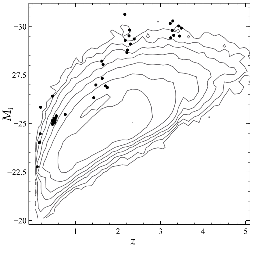
Figure 1: The absolute i-band magnitude vs. redshift for our sample (black dots) plotted against the SDSS DR16 quasar catalog sample (contours).

We cross-matched the optical-UV sample with the Chandra archive for high-quality X-ray imaging spectroscopy in the observed-frame $0.5-10$ keV energy range. To minimize spurious detections, we constrained our sample to objects with an optical-X-ray angular distance ($\Delta_{\rm{Opt-X}}$; i.e., the positional offset between the SDSS and Chandra coordinates) of $<1^{\prime\prime}$, and compiled a final sample of $53$ sources, about half of which are at $z\lesssim 0.8$. This seemingly small number is a consequence of starting off with about three quarters of a million SDSS quasars but only $<1$% of which are at low redshift and have high quality spectral coverage of the C iv region in ultraviolet spectra, and similarly, $<1$% of which are at high redshift and have high quality spectral coverage of the H$\beta$ region. All sources were targeted for Chandra observations, and all but one were observed with the Chandra Advanced CCD Imaging Spectrometer (ACIS; Garmire et al. 2003); SDSS J1119$+$2119 was observed with the Chandra High Resolution Camera (HRC; Murray et al. 1997). Most of the Chandra observations are considered “snapshots” (i.e., $\lesssim 300$ counts), and $\sim 15\%$ of the observations are considered as being “deep” (as can be seen by the sharp drop above $\sim 300$ counts in Figure 2).

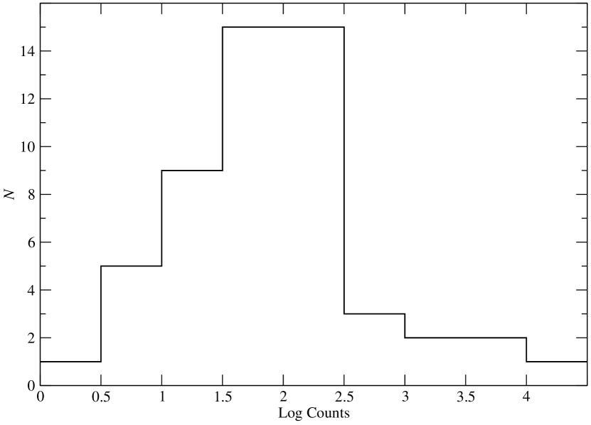
Figure 2: Histogram of the number of counts for each source in the observed-frame $0.5-8$ keV band.

The Chandra observation log appears in Table 1. Column (1) is the SDSS quasar name; Column (2) is the redshift from the SDSS DR16 quasar catalog; Column (3) gives the angular distance between the optical and X-ray positions; Column (4) shows the Galactic absorption column density in units of $10^{20}{\rm cm}^{-2}$, taken from Dickey $\&$ Lockman (1990) and obtained with the HEASARC $N_{\rm H}$ tool; Columns (5) - (8) give the Chandra Cycle, start date, observation ID, and exposure time, respectively.

Source counts were extracted using Chandra Interactive Analysis of Observations (ciao) v4.10 tools. The X-ray counts for all sources except SDSS J1119$+$2119 were obtained using wavdetect (Freeman et al. 2002) with wavelet transforms of scale sizes $1$, $1.4$, $2$, $2.8$, and $4$ pixels, a false-positive probability threshold of $10^{-3}$, and confirmed by visual inspection. Source counts for SDSS J1119$+$2119 were estimated using the ciao dmextract script in the HRC wide band (observed-frame $0.1-10$ keV); the Chandra pimms v4.10 tool was then used to estimate the counts in the energy bands as described below.

Table 1: Chandra Observation Log

		$\Delta_{\rm{Opt-X}}$	Galactic $N_{\rm H}$				Exp. Time
Quasar	$z$	(arcsec)	(1020 cm-2)	Cycle	Obs. Date	Obs. ID	(ks)
(1)	(2)	(3)	(4)	(5)	(6)	(7)	(8)
SDSS J002019.22$-$110609.2 (catalog )	0.49	0.1	2.89	18	2017 Jan 16	19535	3.50
SDSS J005709.94$+$144610.1 (catalog )	0.17	0.1	4.37	1	2000 Jul 28	865	4.66
SDSS J014812.83$+$000322.9 (catalog )	1.48	0.2	2.89	9	2008 Nov 9	9225	10.54
SDSS J015950.23$+$002340.9 (catalog )	0.16	0.8	2.59	4	2003 Aug 26	4104	9.73
SDSS J030341.04$-$002321.9 (catalog )	3.23	0.3	7.14	13	2011 Nov 27	13349	1.54
SDSS J032349.53$-$002949.8 (catalog )	1.63	0.2	6.71	6	2005 Oct 30	5654	8.31
SDSS J080117.79$+$521034.5 (catalog )	3.21	0.6	4.66	15	2014 Dec 11	17081	43.50
SDSS J082024.21$+$233450.4 (catalog )	0.47	0.2	4.02	18	2017 Feb 1	19536	2.95
SDSS J082658.85$+$061142.6 (catalog )	0.50	0.4	2.68	18	2016 Dec 29	19537	3.43
SDSS J083332.92$+$164411.0 (catalog )	0.46	0.3	3.60	18	2017 Oct 12	19538	2.95
SDSS J083510.36$+$035901.1 (catalog )	0.49	0.2	3.29	18	2017 Jun 12	19539	2.95
SDSS J084846.11$+$611234.6 (catalog )	2.26	0.1	4.43	13	2011 Dec 22	13353	1.54
SDSS J085116.14$+$424328.8 (catalog )	0.48	0.3	2.56	18	2017 Jan 15	19540	2.95
SDSS J090033.50$+$421547.0 (catalog )	3.29	0.1	1.99	7	2006 Feb 9	6810	3.91
SDSS J091451.42$+$421957.0 (catalog )	0.55	0.3	1.46	18	2017 Jan 11	19541	3.51
SDSS J093502.52$+$433110.6 (catalog )	0.46	0.2	1.40	18	2017 Jan 12	19542	2.89
SDSS J094202.04$+$042244.5 (catalog )	3.27	0.2	3.56	7	2006 Feb 8	6821	4.07
SDSS J094602.31$+$274407.0 (catalog )	2.44	0.1	1.77	11	2010 Jan 16	11489	4.98
SDSS J094646.94$+$392719.0 (catalog )	2.22	0.3	1.57	12	2011 Feb 27	12857	27.30
SDSS J095852.19$+$120245.0 (catalog )	3.30	0.1	3.22	13	2012 Apr 22	13354	1.56
SDSS J100054.96$+$262242.4 (catalog )	0.51	0.4	2.68	18	2017 Mar 4	19543	3.50
SDSS J102907.09$+$651024.6 (catalog )	2.18	0.2	1.20	9	2008 Jun 17	9228	10.64
SDSS J103320.65$+$274024.2 (catalog )	0.54	0.1	1.87	18	2017 Feb 1	19544	3.51
SDSS J111119.10$+$133603.8 (catalog )	3.48	0.2	1.57	16	2015 Jan 26	17082	43.06
SDSS J111138.66$+$575030.0 (catalog )	0.47	0.2	0.71	18	2017 Aug 31	19545	2.98
SDSS J111830.28$+$402554.0 (catalog )	0.15	$<0.1$	1.91	1	2000 Oct 3	868	19.70
SDSS J111908.67$+$211918.0 (catalog )	0.18	0.3	1.28	3	2002 Jun 29	3145	88.05
SDSS J111941.12$+$595108.7 (catalog )	0.49	0.2	0.73	18	2017 Aug 12	19546	3.54
SDSS J112224.15$+$031802.6 (catalog )	0.47	$<0.1$	4.16	18	2017 Jan 28	19547	2.95
SDSS J112614.93$+$310146.6 (catalog )	0.49	0.1	1.76	18	2017 Jan 23	19548	3.50
SDSS J113327.78$+$032719.1 (catalog )	0.52	0.7	2.74	18	2017 Jan 27	19549	3.43
SDSS J115954.33$+$201921.1 (catalog )	3.43	0.7	2.39	13	2012 Feb 28	13317	1.56
SDSS J123734.47$+$444731.7 (catalog )	0.46	0.1	1.50	18	2017 Mar 3	19551	2.95
SDSS J125415.55$+$480850.6 (catalog )	0.50	0.5	1.12	18	2017 Apr 5	19552	3.05
SDSS J131627.84$+$315825.7 (catalog )	0.46	0.4	1.11	18	2017 Jan 25	19553	3.43
SDSS J134701.54$+$215401.1 (catalog )	0.50	0.3	1.63	18	2017 Mar 22	19554	3.50
SDSS J135023.68$+$265243.1 (catalog )	1.62	0.3	1.23	16	2015 Apr 5	17225	58.76
SDSS J140331.29$+$462804.8 (catalog )	0.46	0.4	1.26	18	2017 Apr 20	19555	2.95
SDSS J140621.89$+$222346.5 (catalog )	0.10	0.3	2.14	1	2000 Jul 22	812	79.12
SDSS J141028.14$+$135950.2 (catalog )	2.21	0.1	1.42	10	2009 Nov 28	10741	4.03
SDSS J141141.96$+$140233.9 (catalog )	1.75	0.1	1.43	14	2012 Dec 16	15353	3.39
SDSS J141730.92$+$073320.7 (catalog )	1.70	0.4	2.12	14	2012 Dec 5	15349	2.48
SDSS J141949.39$+$060654.0 (catalog )	1.64	$<0.1$	2.20	9	2008 Mar 8	9226	9.92
SDSS J141951.84$+$470901.3 (catalog )	2.30	$<0.1$	1.52	3	2002 Jun 2	3076	7.66
SDSS J144741.76$-$020339.1 (catalog )	1.43	0.3	4.53	14	2013 Jan 13	15355	2.00
SDSS J145334.13$+$311401.4 (catalog )	0.46	0.7	1.47	18	2017 Jan 31	19556	2.98
SDSS J152156.48$+$520238.5 (catalog )	2.21	0.9	1.58	14	2013 Oct 22	15334	37.39
SDSS J152654.61$+$565512.3 (catalog )	0.48	0.5	1.42	18	2017 Feb 13	19557	3.50
SDSS J155837.77$+$081345.8 (catalog )	0.52	$<0.1$	3.68	18	2017 Jan 21	19558	3.43
SDSS J212329.46$-$005052.9 (catalog )	2.27	0.5	3.65	16	2015 Dec 22	17080	39.55
SDSS J230301.45$-$093930.7 (catalog )	3.46	0.3	3.32	13	2011 Dec 24	13358	1.54
SDSS J234145.51$-$004640.5 (catalog )	0.52	0.3	3.67	18	2017 Jun 22	19559	3.43
SDSS J235321.62$-$002840.6 (catalog )	0.76	0.1	3.45	7	2006 May 12	6876	2.85

Note. — Column (1) is the SDSS quasar name; Column (2) is the redshift from the SDSS DR16 quasar catalog; Column (3) gives the angular distance between the optical and X-ray positions; Column (4) shows the Galactic absorption column density in units of $10^{20}{\rm cm}^{-2}$, taken from Dickey $\&$ Lockman (1990) and obtained with the HEASARC $N_{\rm H}$ tool; Columns (5) - (8) give the Chandra Cycle, start date, observation ID, and exposure time, respectively.

Table 2 presents the basic X-ray measurements and UV-optical data used for our analyses. Column (1) is the SDSS quasar name; Columns (2) - (4) give the X-ray counts in the soft (observed-frame $0.5-2$ keV), hard (observed-frame $2-8$ keV), and full (observed-frame $0.5-8$ keV) bands, respectively; Column (5) gives the count rate in the soft band; Column (6) gives the Galactic absorption-corrected flux density at rest-frame $2$ keV, assuming a power-law model with $\Gamma=2.0$; Column (7) gives the optical flux density at rest-frame $2500$ Å; Column (8) is the $\alpha_{\rm ox}$ parameter; Column (9) gives the $\Delta$$\alpha_{\rm ox}$ parameter, which is the difference between the measured $\alpha_{\rm ox}$ from Column (8) and the predicted $\alpha_{\rm ox}$, based on the $\alpha_{\rm ox}$-$L_{\nu}(2500\,\text{\AA})$ relation in quasars (given as eq. [3] of Timlin et al. 2020); Column (10) gives the monochromatic luminosity at a rest-frame wavelength of $5100\,\text{\AA}$ [$\nu L_{\nu}(5100\,\text{\AA})$] computed from the flux densities in Column (7), assuming a UV-optical power-law slope of $\alpha_{\rm uv}=-0.5$ (e.g., Vanden Berk et al. 2001); Columns (11) and (12) are the archival measurements and respective references for the FWHM of the broad H$\beta$ line; Column (13) is the Eddington ratio, derived using eq. [2] of Shemmer et al. (2010),

$$L/L_{\rm Edd}=0.13f(L)\left[\frac{\nu L_{\nu}(5100\,\text{\AA})}{10^{44}{\rm~{}erg~{}s}^{-1}}\right]^{0.5}\left[\frac{{\rm FWHM(H}\beta{\rm)}}{10^{3}{\rm~{}km~{}s}^{-1}}\right]^{-2},$$ (1)

where $f(L)$ is the luminosity-dependent bolometric correction to $\nu L_{\nu}(5100\,\text{\AA})$, and was computed using eq. [21] of Marconi et al. (2004); Column (14) gives the rest-frame C iv equivalent width as described below.

The C iv emission line was fit with a local, linear continuum and two independent Gaussian profiles. The linear continuum was constructed using the rest-frame fitting windows $[1445,1465]\,\text{\AA}$ and $[1700,1705]\,\text{\AA}$. The Gaussians were constrained such that the line peak would lie within $5,000$ km s^-1 from the wavelength that corresponded to the maximum flux density of the emission line, the widths could range from $0$ km s^-1 to $15,000$ km s^-1, and the flux density was constrained to up to twice the maximum value of the emission line. Each fit was visually inspected to avoid narrow absorption lines within the C iv profile and noise spikes in the continuum fitting windows. We computed the EW(C iv) values for our sources and compared $21$ of them with the respective values that were available in Shen et al. (2011). The difference between our values and those from Shen et al. (2011), for non-WLQs, is non-systematic and ranges between $|0.8\%|$ and $|33.1\%|$ with a mean value of $|17.5\%|$. The values for the WLQs SDSS J0946$+$2744, SDSS J1411$+$1402, and SDSS J1521$+$5202 differ from those of Shen et al. (2011) by $|196.4\%|$, $|57.5\%|$, and $|204.1\%|$, respectively, which can be attributed to WLQs having extremely low EW(C iv) values with high uncertainties.

=0.25in

Table 2: Basic X-ray and UV-Optical Data

		Counts							$\log\nu L_{\nu}(5100\,\text{\AA})$	FWHM H$\beta$			EW(C iv)
Quasar	$0.5-2$ keV	$2-8$ keV	$0.5-8$ keV	Count Rate	$f_{2~{}\rm keV}$	$f_{2500\,\text{\AA}}$	$\alpha_{\rm ox}$	$\Delta\alpha_{\rm ox}$	(erg s-1)	(km s-1)	Ref.	$L/L_{\rm Edd}$	(Å)
(1)	(2)	(3)	(4)	(5)	(6)	(7)	(8)	(9)	(10)	(11)	(12)	(13)	(14)
SDSS J002019.22$-$110609.2 (catalog )	36.5${}^{+7.1}_{-6.0}$	21.9${}^{+5.8}_{-4.6}$	58.3${}^{+8.7}_{-7.6}$	10.4${}^{+2.0}_{-1.7}$	1.6$\pm{0.3}$	2.4	$-1.60$	$-0.17$	45.1	3105.8	1	0.31	32.1
SDSS J005709.94$+$144610.1 (catalog )	3793.5${}^{+62.6}_{-61.6}$	843.9${}^{+30.1}_{-29.0}$	4632.2${}^{+69.1}_{-68.1}$	814.1${}^{+13.4}_{13.2}$	45.9$\pm{0.7}$	23.5	$-1.42$	$+0.02$	45.1	10011.1	1	0.03	99.2
SDSS J014812.83$+$000322.9 (catalog )	93.8${}^{+10.7}_{-9.7}$	26.8${}^{+6.2}_{-5.1}$	120.4${}^{+12.0}_{-11.0}$	8.9${}^{+1.0}_{-0.9}$	1.3$\pm{0.1}$	1.4	$-1.55$	$+0.02$	45.8	6475.0	2	0.15	15.4
SDSS J015950.23$+$002340.9 (catalog )	3649.5${}^{+61.4}_{-60.4}$	667.3${}^{+26.8}_{-25.8}$	4316.9${}^{+66.7}_{-65.7}$	375.2${}^{+6.3}_{-6.2}$	21.3$\pm{0.4}$	24.6	$-1.56$	$-0.13$	45.1	2406.2	1	0.52	77.1
SDSS J030341.04$-$002321.9 (catalog )	5.0${}^{+3.4}_{-2.1}$	3.9${}^{+3.2}_{-1.9}$	9.0${}^{+4.1}_{-2.9}$	3.2${}^{+2.2}_{-1.4}$	1.0${}^{+0.7}_{-0.4}$	5.5	$-1.82$	$-0.01$	47.0	3010.0	3	2.51	41.0
SDSS J032349.53$-$002949.8 (catalog )	131.8${}^{+12.5}_{-11.5}$	32.7${}^{+6.8}_{-5.7}$	164.4${}^{+13.8}_{-12.8}$	15.9${}^{+1.5}_{-1.4}$	3.0$\pm{0.3}$	2.2	$-1.49$	$+0.14$	46.1	2990.6	2	0.96	48.1
SDSS J080117.79$+$521034.5 (catalog )	116.0${}^{+11.8}_{-10.8}$	49.5${}^{+8.1}_{-7.0}$	168.3${}^{+14.0}_{-13.0}$	2.7${}^{+0.3}_{-0.2}$	0.9$\pm{0.1}$	10.0	$-1.94$	$-0.08$	47.3	5448.7	4	1.07	13.8
SDSS J082024.21$+$233450.4 (catalog )	96.9${}^{+10.9}_{-9.8}$	26.4${}^{+6.2}_{-5.1}$	122.9${}^{+12.1}_{-11.1}$	32.8${}^{+3.7}_{-3.3}$	5.2${}^{+0.6}_{-0.5}$	3.7	$-1.48$	$-0.02$	45.2	2627.0	1	0.48	55.0
SDSS J082658.85$+$061142.6 (catalog )	52.4${}^{+8.3}_{-7.2}$	20.7${}^{+5.6}_{-4.5}$	73.0${}^{+9.6}_{-8.5}$	15.3${}^{+2.4}_{-2.1}$	2.4${}^{+0.4}_{-0.3}$	2.8	$-1.56$	$-0.11$	45.2	1941.0	1	0.88	25.5
SDSS J083332.92$+$164411.0 (catalog )	73.5${}^{+9.6}_{-8.6}$	37.6${}^{+7.2}_{-6.1}$	111.6${}^{+11.6}_{-10.5}$	24.9${}^{+3.3}_{-2.9}$	3.9$\pm{0.5}$	3.4	$-1.51$	$-0.06$	45.2	2954.7	1	0.38	14.6
SDSS J083510.36$+$035901.1 (catalog )	31.6${}^{+6.7}_{-5.6}$	18.7${}^{+5.4}_{-4.3}$	51.1${}^{+8.2}_{-7.1}$	10.7${}^{+2.3}_{-1.9}$	1.7${}^{+0.4}_{-0.3}$	2.8	$-1.62$	$-0.17$	45.2	3479.1	1	0.27	18.2
SDSS J084846.11$+$611234.6 (catalog )	30.3${}^{+6.6}_{-5.5}$	8.8${}^{+4.1}_{-2.9}$	40.0${}^{+7.4}_{-6.3}$	19.7${}^{+4.3}_{-3.6}$	$<4.3$	7.9	$<-1.64$	$<+0.15$	46.9	4280.3	4	1.11	22.0
SDSS J085116.14$+$424328.8 (catalog )	7.0${}^{+3.8}_{-2.6}$	7.0${}^{+3.8}_{-2.6}$	13.9${}^{+4.8}_{-3.7}$	2.4${}^{+1.3}_{-0.9}$	0.4${}^{+0.2}_{-0.1}$	3.3	$-1.90$	$-0.45$	45.2	4468.1	1	0.17	29.0
SDSS J090033.50$+$421547.0 (catalog )	81.1${}^{+10.0}_{-9.0}$	24.7${}^{+6.0}_{-4.9}$	107.5${}^{+11.4}_{-10.3}$	20.8${}^{+2.6}_{-2.3}$	5.2$\pm{0.6}$	9.4	$-1.63$	$+0.23$	47.2	3534.0	3	2.27	40.3
SDSS J091451.42$+$421957.0 (catalog )	20.7${}^{+5.6}_{-4.5}$	7.9${}^{+3.9}_{-2.7}$	28.5${}^{+6.4}_{-5.3}$	5.9${}^{+1.6}_{-1.3}$	0.9${}^{+0.3}_{-0.2}$	2.6	$-1.71$	$-0.25$	45.2	2945.6	1	0.38	65.1
SDSS J093502.52$+$433110.6 (catalog )	320.6${}^{+18.9}_{-17.9}$	159.5${}^{+13.7}_{-12.6}$	478.8${}^{+22.9}_{-21.9}$	110.9${}^{+6.5}_{-6.2}$	16.7${}^{+1.0}_{-0.9}$	13.1	$-1.50$	$+0.06$	45.8	8467.4	1	0.09	46.2
SDSS J094202.04$+$042244.5 (catalog )	32.7${}^{+6.8}_{-5.7}$	9.8${}^{+4.2}_{-3.1}$	43.5${}^{+7.7}_{-6.6}$	8.0${}^{+1.7}_{-1.4}$	2.1$\pm{0.4}$	6.1	$-1.71$	$+0.11$	47.1	4396.0	3	1.31	35.0
SDSS J094602.31$+$274407.0 (catalog )	4.0${}^{+3.2}_{-1.9}$	$<4.8$	5.0${}^{+3.4}_{-2.1}$	0.8${}^{+0.6}_{-0.4}$	0.2$\pm{0.1}$	7.1	$-2.16$	$-0.37$	46.9	4819.0	4	0.88	8.3
SDSS J094646.94$+$392719.0 (catalog )	13.9${}^{+4.8}_{-3.7}$	6.8${}^{+3.7}_{-2.5}$	20.6${}^{+5.6}_{-4.5}$	0.5${}^{+0.2}_{-0.1}$	0.1$\pm{0.0}$	3.1	$-2.11$	$-0.40$	46.5	4966.0	4	0.54	19.9
SDSS J095852.19$+$120245.0 (catalog )	15.8${}^{+5.1}_{-3.9}$	2.0${}^{+2.6}_{-1.3}$	20.8${}^{+5.6}_{-4.5}$	10.2${}^{+3.3}_{-2.5}$	2.9${}^{+0.9}_{-0.7}$	4.4	$-1.61$	$+0.19$	46.9	4505.7	4	1.01	30.8
SDSS J100054.96$+$262242.4 (catalog )	33.2${}^{+6.8}_{-5.7}$	13.7${}^{+4.8}_{-3.6}$	47.7${}^{+8.0}_{-6.9}$	9.5${}^{+2.0}_{-1.6}$	1.5$\pm{0.3}$	2.8	$-1.64$	$-0.19$	45.2	1798.7	1	1.02	13.6
SDSS J102907.09$+$651024.6 (catalog )	114.1${}^{+11.7}_{-10.7}$	24.6${}^{+6.0}_{-4.9}$	139.4${}^{+12.8}_{-11.8}$	10.7${}^{+1.1}_{-1.0}$	1.9$\pm{0.2}$	5.4	$-1.71$	$+0.04$	46.7	4770.0	4	0.72	26.2
SDSS J103320.65$+$274024.2 (catalog )	34.4${}^{+6.9}_{-5.8}$	24.8${}^{+6.1}_{-4.9}$	59.2${}^{+8.7}_{-7.7}$	9.8${}^{+2.0}_{-1.7}$	1.6$\pm{0.3}$	2.6	$-1.62$	$-0.17$	45.2	5077.0	1	0.13	49.6
SDSS J111119.10$+$133603.8 (catalog )	134.5${}^{+12.6}_{-11.6}$	45.2${}^{+7.8}_{-6.7}$	179.5${}^{+14.4}_{-13.4}$	3.1$\pm{0.3}$	1.1$\pm{0.1}$	7.0	$-1.84$	$0.00$	47.2	6919.0	4	0.59	18.9
SDSS J111138.66$+$575030.0 (catalog )	36.4${}^{+7.1}_{-6.0}$	9.9${}^{+4.3}_{-3.1}$	46.4${}^{+7.9}_{-6.8}$	12.2${}^{+2.4}_{-2.0}$	1.8${}^{+0.4}_{-0.3}$	3.4	$-1.64$	$-0.19$	45.2	1676.4	1	1.18	37.6
SDSS J111830.28$+$402554.0 (catalog )	1814.5${}^{+43.6}_{-42.6}$	543.9${}^{+24.3}_{-23.3}$	2355.5${}^{+49.5}_{-48.5}$	92.1$\pm{2.2}$	7.8$\pm{0.2}$	18.6	$-1.68$	$-0.28$	44.9	4057.0	1	0.15	47.2
SDSS J111908.67$+$211918.0 (catalog )	11630$\pm{150}$	987$\pm{13}$	12620$\pm{170}$	130$\pm{2}$	159.5$\pm{2.1}$	72.4	$-1.40$	$+0.12$	45.7	2920.0	5	0.62	65.8
SDSS J111941.12$+$595108.7 (catalog )	16.5${}^{+5.2}_{-4.0}$	8.0${}^{+4.0}_{-2.8}$	26.4${}^{+6.2}_{-5.1}$	4.7${}^{+1.5}_{-1.1}$	0.7$\pm{0.2}$	2.7	$-1.76$	$-0.32$	45.1	1501.6	1	1.33	22.4
SDSS J112224.15$+$031802.6 (catalog )	12.6${}^{+4.7}_{-3.5}$	13.8${}^{+4.8}_{-3.7}$	26.4${}^{+6.2}_{-5.1}$	4.3${}^{+1.6}_{-1.2}$	0.7${}^{+0.3}_{-0.2}$	3.4	$-1.80$	$-0.35$	45.2	3214.1	1	0.32	22.4
SDSS J112614.93$+$310146.6 (catalog )	87.8${}^{+10.4}_{-9.4}$	31.5${}^{+6.7}_{-5.6}$	119.3${}^{+12.0}_{-10.9}$	25.1${}^{+3.0}_{-2.7}$	3.9${}^{+0.5}_{-0.4}$	2.3	$-1.44$	$-0.01$	45.1	4005.0	1	0.19	65.1
SDSS J113327.78$+$032719.1 (catalog )	87.5${}^{+10.4}_{-9.3}$	28.4${}^{+6.4}_{-5.3}$	119.2${}^{+12.0}_{-10.9}$	25.5${}^{+3.0}_{-2.7}$	4.1${}^{+0.5}_{-0.4}$	2.9	$-1.48$	$-0.02$	45.2	4062.9	1	0.20	137.3
SDSS J115954.33$+$201921.1 (catalog )	$<6.4$	$<4.8$	3.0${}^{+2.9}_{-1.6}$	$<4.1$	$<1.2$	7.6	$<-1.85$	$<0.00$	47.2	6599.0	3	0.65	24.8
SDSS J123734.47$+$444731.7 (catalog )	72.3${}^{+9.5}_{-8.5}$	28.9${}^{+6.4}_{-5.3}$	101.1${}^{+11.1}_{-10.0}$	24.5${}^{+3.2}_{-2.9}$	3.7${}^{+0.5}_{-0.4}$	3.9	$-1.54$	$-0.08$	45.2	4257.5	1	0.18	23.1
SDSS J125415.55$+$480850.6 (catalog )	103.7${}^{+11.2}_{-10.2}$	49.6${}^{+8.1}_{-7.0}$	154.0${}^{+13.4}_{-12.4}$	34.0${}^{+3.7}_{-3.3}$	5.2${}^{+0.6}_{-0.5}$	3.5	$-1.47$	$0.00$	45.3	3597.7	1	0.28	55.7
SDSS J131627.84$+$315825.7 (catalog )	$<3.0$	4.0${}^{+3.2}_{-1.9}$	4.0${}^{+3.2}_{-1.9}$	$<0.9$	$<0.1$	2.6	$<-2.03$	$<-0.60$	45.1	2589.4	1	0.45	44.4
SDSS J134701.54$+$215401.1 (catalog )	69.7${}^{+9.4}_{-8.3}$	19.6${}^{+5.5}_{-4.4}$	89.2${}^{+10.5}_{-9.4}$	19.9${}^{+2.7}_{-2.4}$	3.1$\pm{0.4}$	2.2	$-1.48$	$-0.05$	45.1	2201.1	1	0.62	51.8
SDSS J135023.68$+$265243.1 (catalog )	264.5${}^{+17.3}_{-16.3}$	133.4${}^{+12.6}_{-11.5}$	396.7${}^{+20.9}_{-19.9}$	4.5$\pm{0.3}$	1.5$\pm{0.1}$	4.3	$-1.71$	$-0.02$	46.4	3813.0	6	0.81	30.8
SDSS J140331.29$+$462804.8 (catalog )	8.0${}^{+4.0}_{-2.8}$	8.9${}^{+4.1}_{-2.9}$	17.8${}^{+5.3}_{-4.2}$	2.7${}^{+1.3}_{-0.9}$	0.4${}^{+0.2}_{-0.1}$	3.0	$-1.87$	$-0.43$	45.1	2459.4	1	0.49	73.9
SDSS J140621.89$+$222346.5 (catalog )	1290.0${}^{+36.9}_{-35.9}$	325.2${}^{+19.1}_{-18.0}$	1620.8${}^{+41.3}_{-40.3}$	16.3$\pm{0.5}$	11.6$\pm{0.4}$	10.8	$-1.52$	$-0.25$	44.3	1524.9	1	0.58	34.1
SDSS J141028.14$+$135950.2 (catalog )	49.2${}^{+8.1}_{-7.0}$	14.8${}^{+4.9}_{-3.8}$	63.8${}^{+9.0}_{-8.0}$	12.2${}^{+2.0}_{-1.7}$	2.2${}^{+0.4}_{-0.3}$	4.9	$-1.67$	$+0.08$	46.7	5565.0	4	0.53	31.4
SDSS J141141.96$+$140233.9 (catalog )	46.6${}^{+7.9}_{-6.8}$	11.8${}^{+4.5}_{-3.4}$	58.3${}^{+8.7}_{-7.6}$	13.7${}^{+2.3}_{-2.0}$	2.3${}^{+0.4}_{-0.3}$	1.1	$-1.42$	$+0.16$	45.9	3966.0	7	0.44	4.3
SDSS J141730.92$+$073320.7 (catalog )	20.8${}^{+5.6}_{-4.5}$	4.9${}^{+3.4}_{-2.1}$	25.6${}^{+6.1}_{-5.0}$	8.4${}^{+2.3}_{-1.8}$	1.4${}^{+0.4}_{-0.3}$	1.6	$-1.56$	$+0.05$	46.0	2784.0	7	0.99	1.4
SDSS J141949.39$+$060654.0 (catalog )	93.1${}^{+10.7}_{-9.6}$	11.9${}^{+4.6}_{-3.4}$	105.9${}^{+11.3}_{-10.3}$	9.4${}^{+1.1}_{-1.0}$	1.4$\pm{0.2}$	3.0	$-1.66$	$0.00$	46.2	5252.0	6	0.35	21.4
SDSS J141951.84$+$470901.3 (catalog )	125.1${}^{+12.2}_{-11.2}$	28.7${}^{+6.4}_{-5.3}$	154.4${}^{+13.5}_{-12.4}$	16.3${}^{+1.6}_{-1.5}$	2.3$\pm{0.2}$	6.2	$-1.70$	$+0.07$	46.8	4816.0	4	0.79	23.2
SDSS J144741.76$-$020339.1 (catalog )	4.9${}^{+3.4}_{-2.1}$	$<4.8$	5.9${}^{+3.6}_{-2.4}$	2.4${}^{+1.7}_{-1.1}$	0.4${}^{+0.3}_{-0.2}$	1.7	$-1.78$	$-0.20$	45.9	1923.0	7	1.87	7.7
SDSS J145334.13$+$311401.4 (catalog )	6.0${}^{+4.0}_{-2.4}$	17.7${}^{+5.3}_{-4.2}$	23.7${}^{+5.9}_{-4.8}$	2.0${}^{+1.2}_{-0.8}$	0.3${}^{+0.2}_{-0.1}$	3.9	$-1.96$	$-0.50$	45.3	4936.1	1	0.15	51.1
SDSS J152156.48$+$520238.5 (catalog )	41.7${}^{+7.5}_{-6.4}$	43.0${}^{+7.6}_{-6.5}$	84.7${}^{+10.2}_{-9.2}$	1.1$\pm{0.2}$	0.2$\pm{0.04}$	19.9	$-2.29$	$-0.43$	47.3	5750.0	8	0.96	9.0
SDSS J152654.61$+$565512.3 (catalog )	44.6${}^{+7.7}_{-6.6}$	22.5${}^{+5.8}_{-4.7}$	67.0${}^{+9.2}_{-8.2}$	12.7${}^{+2.2}_{-1.9}$	1.9$\pm{0.3}$	2.7	$-1.59$	$-0.15$	45.1	2690.7	1	0.41	50.1
SDSS J155837.77$+$081345.8 (catalog )	30.6${}^{+6.6}_{-5.5}$	23.6${}^{+5.9}_{-4.8}$	54.2${}^{+8.4}_{-7.3}$	8.9${}^{+1.9}_{-1.6}$	1.5$\pm{0.3}$	2.7	$-1.64$	$-0.19$	45.2	2429.7	1	0.56	40.5
SDSS J212329.46$-$005052.9 (catalog )	548.0${}^{+24.4}_{-23.4}$	195.4${}^{+15.0}_{-14.0}$	741.6${}^{+28.2}_{-27.2}$	13.9$\pm{0.6}$	3.9$\pm{0.2}$	14.5	$-1.75$	$+0.09$	47.2	4500.0	9	1.40	18.5
SDSS J230301.45$-$093930.7 (catalog )	4.8${}^{+3.4}_{-2.1}$	$<3.0$	5.7${}^{+3.5}_{-2.3}$	3.1${}^{+2.2}_{-1.4}$	0.9${}^{+0.6}_{-0.4}$	4.4	$-1.80$	$0.00$	47.0	5887.0	3	0.66	18.7
SDSS J234145.51$-$004640.5 (catalog )	29.6${}^{+6.5}_{-5.4}$	28.4${}^{+6.4}_{-5.3}$	58.9${}^{+8.7}_{-7.7}$	8.6${}^{+1.9}_{-1.6}$	1.4$\pm{0.3}$	2.7	$-1.65$	$-0.20$	45.2	6152.5	1	0.09	62.0
SDSS J235321.62$-$002840.6 (catalog )	81.9${}^{+10.1}_{-9.0}$	26.6${}^{+6.2}_{-5.1}$	108.3${}^{+11.4}_{-10.4}$	28.7${}^{+3.5}_{-3.2}$	3.1${}^{+0.4}_{-0.3}$	1.8	$-1.44$	$+0.04$	45.4	3808.4	1	0.28	99.1

Note. — Column (1) is the SDSS quasar name; Columns (2) - (4) give the X-ray counts in the soft (observed-frame $0.5-2$ keV), hard (observed-frame $2-8$ keV), and full (observed-frame $0.5-8$ keV) bands, respectively; Column (5) gives the count rate in the soft band in units of $10^{-3}$ counts s^-1; Column (6) gives the Galactic absorption-corrected flux density at rest-frame $2$ keV in units of $10^{-31}$ erg cm^-2 s^-1 Hz^-1, assuming a power-law model with $\Gamma=2.0$; Column (7) gives the optical flux density at rest-frame $2500$ Å with units of $10^{-27}$ erg cm^-2 s^-1 Hz^-1, obtained from Shen et al. (2011) and corrected for Galactic extinction unless otherwise noted; Column (8) is the $\alpha_{\rm ox}$ parameter; Column (9) gives the $\Delta$$\alpha_{\rm ox}$ parameter, which is the difference between the measured $\alpha_{\rm ox}$ from Column (8) and the predicted $\alpha_{\rm ox}$, based on the $\alpha_{\rm ox}$-$L_{\nu}(2500\,\text{\AA})$ relation in quasars (given as eq. [3] of Timlin et al. 2020); Column (10) gives the monochromatic luminosity at a rest-frame wavelength of $5100\,\text{\AA}$ [$\nu L_{\nu}(5100\,\text{\AA})$] computed from the flux densities in Column (7), assuming a UV-optical power-law slope of $\alpha_{\rm uv}=-0.5$ (e.g., Vanden Berk et al. 2001); Columns (11) and (12) are the archival measurements and respective references for the FWHM of the broad H$\beta$ line; Column (13) is the Eddington ratio, derived using eq. [2] of Shemmer et al. (2010); Column (14) gives the rest-frame C iv equivalent width as described in the text.

References. — Rest-frame optical data obtained from: (1) Shen et al. (2011); (2) Mejia-Restrepo et al. (2016); (3) Zuo et al. (2015); (4) Matthews et al. (2021); (5) Boroson & Green (1992); (6) Shen & Liu (2012); (7) Plotkin et al. (2015); (8) Wu et al. (2011); (9) Dix et al. (2020).

3 Results and Discussion

Our goal is to test whether X-ray data can strengthen current optical-UV indicators of $L/L_{\rm Edd}$ such as those provided by the C iv spectroscopic parameter space. The following provides a step-by-step description of the analyses performed to test this hypothesis.

Figure 3 shows a significant anti-correlation between EW(C iv) and H$\beta$-based $L/L_{\rm Edd}$ for our sources, with a Spearman-rank correlation coefficient ($r_{s}$) of $-0.42$ and a chance probability ($p$) of $1.8\times 10^{-3}$, confirming the results of Shemmer & Lieber (2015). We find that two of our sources deviate significantly ($\gtrsim 4\sigma$) from this correlation; these are SDSS J1411$+$1402 and SDSS J1417$+$0733, which are WLQs with EW(C iv) values of $4.3\,\text{\AA}$ and $1.4\,\text{\AA}$, respectively. However, the exclusion of these sources does not significantly impact the correlation ($r_{s}=-0.43$, $p=1.7\times 10^{-3}$). To test whether X-ray information can minimize the scatter in this correlation, symbol sizes in Figure 3 (a) depend on the objects’ $\alpha_{\rm ox}$ values, and symbol sizes in Figure 3 (b) depend on $\Delta\alpha_{\rm ox}$. We do not find any trends stemming from this sorting by $\alpha_{\rm ox}$ or $\Delta\alpha_{\rm ox}$. We also ran partial correlations distinguishing between X-ray strong (weak) sources if these are above (below) the median $\alpha_{\rm ox}$ for our sample which is $-1.64$; these correlation coefficients and chance probabilities are shown in Table 3. We find a stronger anti-correlation for the X-ray weak sources ($r_{s}=-0.55$, $p=4.0\times 10^{-3}$) than the X-ray strong sources ($r_{s}=-0.26$, $p=0.18$), which can be seen in Figure 3 (c).

To investigate whether our sample is biased with respect to the $\alpha_{\rm ox}$ diagnostic, in Figure 4 we show $\alpha_{\rm ox}$ and $\Delta\alpha_{\rm ox}$ vs $L_{2500\,\text{\AA}}$ (left), H$\beta$-based $L/L_{\rm Edd}$  (center), and EW(C iv) (right). In spite of the fact that no significant evolution in the X-ray properties of quasars has been observed across cosmic time (e.g., Shemmer et al. 2005; Nanni et al. 2017; Vito et al. 2019), we also ran partial correlations after sorting our sample by luminosity, creating “Low $L$” and “High $L$” subsets with Low $L$ corresponding to the low redshift ($z<0.8$) sources and defined as $\log L_{2500\,\text{\AA}}<30.7$ erg s^-1 Hz^-1. Spearman-rank correlation coefficients and chance probabilities for the full sample and each sub-sample are also presented in Table 3.

Table 3: $\alpha_{\rm ox}$($\Delta\alpha_{\rm ox}$) Spearman-rank Partial Correlations

vs.	Control	$r_{s}$	$p$
(1)	(2)	(3)	(4)
Full Sample (53 sources)
$L_{2500\,\text{\AA}}$		$-0.40$ ($+0.50$)	0.003 ($\mathbf{1.3\times 10^{-4}}$)
$L_{2500\,\text{\AA}}$	$L/L_{\rm Edd}$	$-0.27$ ($+0.47$)	0.05 ($\mathbf{5.1\times 10^{-4}}$)
$L_{2500\,\text{\AA}}$	EW(C iv)	$-0.28$ ($+0.54$)	0.04 ($<0.0001$)
$L/L_{\rm Edd}$		$-0.34$ ($+0.22$)	0.01 ($>0.05$)
$L/L_{\rm Edd}$	$L_{2500\,\text{\AA}}$	$-0.18$ ($-0.05$)	$>0.05$ ($>0.05$)
$L/L_{\rm Edd}$	EW(C iv)	$-0.23$ ($+0.22$)	$>0.05$ ($>0.05$)
EW(C iv)		$+0.36$ ($-0.05$)	0.008 ($>0.05$)
EW(C iv)	$L_{2500\,\text{\AA}}$	$+0.23$ ($+0.22$)	$>0.05$ ($>0.05$)
EW(C iv)	$L/L_{\rm Edd}$	$+0.26$ ($+0.04$)	$>0.05$ ($>0.05$)
Low $L$ (29 sources)
$L_{2500\,\text{\AA}}$		$+0.12$ ($+0.25$)	$>0.05$ ($>0.05$)
$L_{2500\,\text{\AA}}$	$L/L_{\rm Edd}$	$+0.12$ ($+0.24$)	$>0.05$ ($>0.05$)
$L_{2500\,\text{\AA}}$	EW(C iv)	$+0.06$ ($+0.21$)	$>0.05$ ($>0.05$)
$L/L_{\rm Edd}$		$-0.02$ ($-0.06$)	$>0.05$ ($>0.05$)
$L/L_{\rm Edd}$	$L_{2500\,\text{\AA}}$	$+0.004$ ($-0.01$)	$>0.05$ ($>0.05$)
$L/L_{\rm Edd}$	EW(C iv)	$+0.10$ ($+0.06$)	$>0.05$ ($>0.05$)
EW(C iv)		$+0.40$ ($+0.41$)	0.03 (0.03)
EW(C iv)	$L_{2500\,\text{\AA}}$	$+0.39$ ($+0.39$)	0.04 (0.04)
EW(C iv)	$L/L_{\rm Edd}$	$+0.41$ ($+0.41$)	0.03 (0.03)
High $L$ (24 sources)
$L_{2500\,\text{\AA}}$		$-0.62$ ($-0.09$)	0.001 ($>0.05$)
$L_{2500\,\text{\AA}}$	$L/L_{\rm Edd}$	$-0.61$ ($-0.17$)	0.002 ($>0.05$)
$L_{2500\,\text{\AA}}$	EW(C iv)	$-0.66$ ($-0.13$)	$\mathbf{5.9\times 10^{-4}}$ ($>0.05$)
$L/L_{\rm Edd}$		$-0.20$ ($+0.12$)	$>0.05$ ($>0.05$)
$L/L_{\rm Edd}$	$L_{2500\,\text{\AA}}$	$+0.16$ ($+0.18$)	$>0.05$ ($>0.05$)
$L/L_{\rm Edd}$	EW(C iv)	$-0.22$ ($+0.09$)	$>0.05$ ($>0.05$)
EW(C iv)		$+0.27$ ($+0.39$)	$>0.05$ ($>0.05$)
EW(C iv)	$L_{2500\,\text{\AA}}$	$+0.39$ ($+0.40$)	$>0.05$ ($>0.05$)
EW(C iv)	$L/L_{\rm Edd}$	$+0.29$ ($+0.39$)	$>0.05$ ($>0.05$)
X-ray Weak (26 sources)
$L_{2500\,\text{\AA}}$		$-0.27$ ($+0.54$)	$>0.05$ (0.005)
$L_{2500\,\text{\AA}}$	$L/L_{\rm Edd}$	$-0.27$ ($+0.42$)	$>0.05$ (0.04)
$L_{2500\,\text{\AA}}$	EW(C iv)	$-0.20$ ($+0.54$)	$>0.05$ (0.006)
$L/L_{\rm Edd}$		$-0.08$ ($+0.39$)	$>0.05$ (0.05)
$L/L_{\rm Edd}$	$L_{2500\,\text{\AA}}$	$+0.08$ ($+0.15$)	$>0.05$ ($>0.05$)
$L/L_{\rm Edd}$	EW(C iv)	$+0.05$ ($+0.38$)	$>0.05$ ($>0.05$)
EW(C iv)		$+0.21$ ($-0.15$)	$>0.05$ ($>0.05$)
EW(C iv)	$L_{2500\,\text{\AA}}$	$+0.10$ ($+0.15$)	$>0.05$ ($>0.05$)
EW(C iv)	$L/L_{\rm Edd}$	$+0.20$ ($+0.09$)	$>0.05$ ($>0.05$)
X-ray Strong (27 sources)
$L_{2500\,\text{\AA}}$		$-0.07$ ($+0.79$)	$>0.05$ $\mathbf{(<0.0001)}$
$L_{2500\,\text{\AA}}$	$L/L_{\rm Edd}$	$+0.05$ ($+0.78$)	$>0.05$ $\mathbf{(<0.0001)}$
$L_{2500\,\text{\AA}}$	EW(C iv)	$+0.07$ ($+0.81$)	$>0.05$ $\mathbf{(<0.0001)}$
$L/L_{\rm Edd}$		$-0.39$ ($+0.17$)	0.04 ($>0.05$)
$L/L_{\rm Edd}$	$L_{2500\,\text{\AA}}$	$-0.39$ ($-0.09$)	0.05 ($>0.05$)
$L/L_{\rm Edd}$	EW(C iv)	$-0.32$ ($+0.17$)	$>0.05$ ($>0.05$)
EW(C iv)		$+0.45$ ($-0.02$)	0.02 ($>0.05$)
EW(C iv)	$L_{2500\,\text{\AA}}$	$+0.45$ ($+0.33$)	0.02 ($>0.05$)
EW(C iv)	$L/L_{\rm Edd}$	$+0.39$ ($+0.03$)	0.05 ($>0.05$)

Note. — Column (1) is the parameter that was correlated with $\alpha_{\rm ox}$ ($\Delta\alpha_{\rm ox}$); Column (2) is the controlled parameter - If entry is empty, we only calculated the correlation between $\alpha_{\rm ox}$ ($\Delta\alpha_{\rm ox}$) and the parameter in the first column; otherwise, we calculated the partial correlation between $\alpha_{\rm ox}$ ($\Delta\alpha_{\rm ox}$) and the parameter in the first column while controlling for the parameter in the second column; Columns (3) and (4) are the Spearman-rank correlation coefficient and chance probability, respectively. Significant correlations are shown in bold and defined as $p<0.05$. Low $L$ (High $L$) corresponds to objects with $\log L_{2500\,\text{\AA}}$ below (above) $30.7$ erg s^-1 Hz^-1. X-ray weak (strong) corresponds to objects with an $\alpha_{\rm ox}$ value below (above) the median value of $-1.64$.

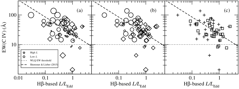
Figure 3: The EW(C iv) vs. $L/L_{\rm Edd}$ anti-correlation. For panels (a) and (b), circles represent the Low $L$ sources ($\log L_{2500\,\text{\AA}}<30.7$ erg s^-1 Hz^-1) and diamonds represent the High $L$ sources. Larger symbol sizes correspond to sources with larger (i.e., less negative) $\alpha_{\rm ox}$ values in (a). In (b), symbol sizes denote the $\sigma$ values of $\Delta\alpha_{\rm ox}$, with the largest symbols corresponding to $\Delta\alpha_{\rm ox}$ values within 1$\sigma$ ($\pm{0.131}$; e.g., Just et al. 2007). In (c), squares (pluses) represent objects with an $\alpha_{\rm ox}$ value below (above) the median value of $-1.64$. The dotted lines show the $10\,\text{\AA}$ EW threshold for defining WLQs (Diamond-Stanic et al. 2009), and the dashed lines show the regression lines corresponding to Equation [2] of Shemmer & Lieber (2015). It appears that the additional X-ray information does not contribute any new trends to the data.

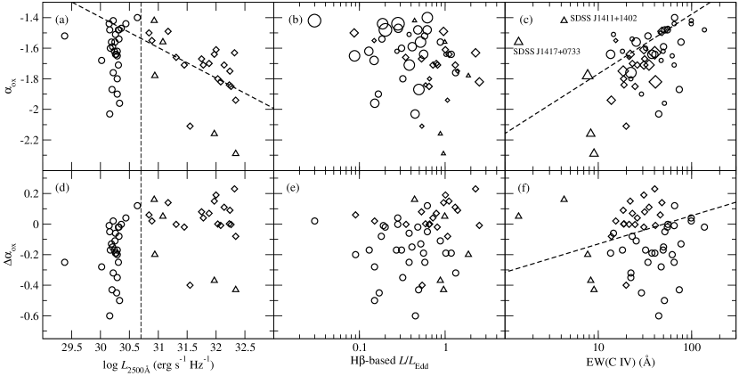
Figure 4: Optical-to-X-ray spectral slope ($\alpha_{\rm ox}$) (top) and $\Delta\alpha_{\rm ox}$ (bottom) vs $L_{2500\,\text{\AA}}$ (left), H$\beta$-based $L/L_{\rm Edd}$ (center), and EW(C iv) (right). Circles represent the Low $L$ sources, diamonds represent the High $L$ sources, and triangles represent WLQs (all of which are included in the High $L$ sub-sample); the threshold between low and high luminosity is shown by the vertical dashed line in panels (a) and (d). The bold dashed lines in panels (a), (c), and (f) show the best fit relations found in Timlin et al. (2020). Symbol sizes in panels (b) and (c) denote the EW(C iv) and $L/L_{\rm Edd}$ values, respectively, with larger symbols corresponding to larger values. Our High $L$ sources appear to follow the $\alpha_{\rm ox}$-$L_{2500\,\text{\AA}}$ relation of Timlin et al. (2020), however our Low $L$ sources seem to spoil the relation, presumably given the selection bias inherent in the majority of these sources as explained in the text.

We find a significant anti-correlation between $\alpha_{\rm ox}$ and $L_{2500\,\text{\AA}}$ consistent with previous studies (e.g., Timlin et al. 2020), which becomes stronger with the exclusion of our $29$ Low $L$ objects (see Table 3). This deviation may be due to the $\alpha_{\rm ox}$-$L_{2500\,\text{\AA}}$ relation breaking down at some low $L_{2500\,\text{\AA}}$ value, which could also lead to the very low $\Delta\alpha_{\rm ox}$ values in some of our low luminosity objects (see Figure 4). The additional exclusion of the X-ray weak, high-luminosity source SDSS J0946$+$3927 as well as WLQs SDSS J0946$+$2744 and SDSS J1521$+$5202, gives an even stronger correlation with $r_{s}=-0.68$ and $p=6.3\times 10^{-4}$ (see Figure 4).

One notable finding in Table 3 is the apparent strong $\Delta\alpha_{\rm ox}$-$L_{2500\,\text{\AA}}$ correlation for the full sample as well as the X-ray strong sources. The corresponding significantly smaller correlation coefficients found in the High $L$/ Low $L$ and X-ray weak sub-samples, as well as visual inspection of Figure 4, suggest that such a strong correlation is not to be expected. Direct comparison with other samples (e.g., Steffen et al. 2006; Just et al. 2007) confirms that our results for the High $L$/Low $L$ and X-ray weak sources are consistent with the trends found in previous studies. Therefore, the strong $\Delta\alpha_{\rm ox}$-$L_{2500\,\text{\AA}}$ correlation may be due to a small sample bias as well as the significant scatter (or the breakdown of the $\alpha_{\rm ox}$-$L_{2500\,\text{\AA}}$ correlation) at low luminosity (see Figure 4 (a) and (d)), which is related to a bias in favor of low-luminosity sources and the way they were selected as discussed further below.

The increased scatter at low luminosity may also have a contribution from larger amplitudes of X-ray variability which, together with the fact that the X-ray and optical-UV measurements are non-contemporaneous, would produce uncertainties on the order of $\Delta\alpha_{\rm ox}$$\gtrsim 0.1$ (e.g., Vagnetti et al. 2010, 2013). To investigate the potential effects of variability further, we examined the Chandra observations of the eight sources that have $>300$ counts in the full band (i.e., non-“snapshots”; see Section 2, Figure 2, and Table 2). We split each of these observations into two sub-exposures with equal exposure times and compared the count rates between the two sub-exposures; the rest-frame time difference between each pair of sub-exposures is in the range $\sim 1-10$ hr. We found that in all cases the count rates in both sub-exposures were consistent with each other, within the errors, indicating the absence of short-term variability.

For the full sample and High $L$ sub-sample, we find that the correlations between $\alpha_{\rm ox}$ and $L/L_{\rm Edd}$ are weaker than the respective $\alpha_{\rm ox}$-$L_{2500\,\text{\AA}}$ correlations (see Table 3). These weaker correlations may be due to the inherent dependence of $L/L_{\rm Edd}$ on $L_{2500\,\text{\AA}}$ and black-hole mass and the additional uncertainties associated with estimating $L/L_{\rm Edd}$ (see, e.g., Shemmer et al. 2008). To see if the EW(C iv) parameter contributes to this anti-correlation, Figure 4 (b) shows larger symbols that correspond to larger values of EW(C iv); however no trend with EW(C iv) has been found.

We find that the correlation between $\alpha_{\rm ox}$ and EW(C iv) for the full sample is stronger than the corresponding $\alpha_{\rm ox}$-$L/L_{\rm Edd}$ correlation, yet not as strong as the $\alpha_{\rm ox}$-$L_{2500\,\text{\AA}}$ correlation (see Table 3). As can be seen in Figure 4, there are two sources that are significant outliers; these are the WLQs SDSS J1411$+$1402 and SDSS J1417$+$0733. Comparison with Luo et al. (2015) shows the same $\alpha_{\rm ox}$ values as those calculated in this work, and exclusion of these sources significantly improves the correlation to $r_{s}=0.41$ and $p=4.3\times 10^{-3}$. The $\alpha_{\rm ox}$-EW(C iv) correlation also seems to hold in almost any subsample (see Table 3), notwithstanding effects due to changing sample size, which supports the results of Timlin et al. (2021) that $\alpha_{\rm ox}$ is expected to be correlated with EW(C iv) as an indicator of the shape of the spectral energy distribution. To see if the $L/L_{\rm Edd}$ parameter contributes to this correlation, Figure 4 (c) shows larger symbols that correspond to larger values of $L/L_{\rm Edd}$; however no trend with $L/L_{\rm Edd}$ has been found.

Overall, Table 3 shows a significant difference between the Low $L$ and High $L$ sub-samples with respect to the $\alpha_{\rm ox}$ ($\Delta\alpha_{\rm ox}$) vs. $L_{2500\,\text{\AA}}$ and $L/L_{\rm Edd}$ correlations. The Low $L$ sources do not exhibit significant correlations between $L_{2500\,\text{\AA}}$ or $L/L_{\rm Edd}$ and $\alpha_{\rm ox}$ and, therefore, spoil the correlations for the entire sample. This difference may be a consequence of the fact that most of these sources were originally selected to have a small range in $L_{2500\,\text{\AA}}$, but a large range in the accretion-rate diagnostics FWHM(H$\beta$) and R(Fe ii) (see Rivera et al. 2022, under review), which likely contribute to the large range in $\alpha_{\rm ox}$.

The X-ray weak sub-sample exhibits the same trends as the High $L$ sub-sample, namely that the $\alpha_{\rm ox}$-$L_{2500\,\text{\AA}}$ correlations are the strongest, and the $\alpha_{\rm ox}$-$L/L_{\rm Edd}$ correlations are the weakest; while the X-ray strong sub-sample shares one trend with the Low $L$ sub-sample, in which the $\alpha_{\rm ox}$-EW(C iv) correlations are the strongest.

To quantify the potential contribution of the $\alpha_{\rm ox}$ parameter to the Eddington ratio estimate, a multiple regression analysis was performed using the $L/L_{\rm Edd}$ values from Table 2 as the dependent variable, and the $\alpha_{\rm ox}$, $L_{2500\,\text{\AA}}$, and EW(C iv) values from Table 2 as the independent variables. These regressions include combinations of the above parameters with linear, interaction, and quadratic terms; each with and without an intercept. The results of these regressions suggest that $\alpha_{\rm ox}$ does not contribute significantly to creating a diagnostic to $L/L_{\rm Edd}$ for our entire sample. The linear model with the best fit has the form:

$$\begin{gathered}\small L/L_{\rm Edd}=\alpha+\beta\,\text{$\alpha_{\rm ox}$}+\gamma\,\text{{\rm log}~{}$L_{2500\,\text{\AA}}$}+\delta\,\text{EW(C~{}{\sc iv})}\end{gathered}$$ (2)

where

$$\begin{gathered}\alpha=-9.0\pm{2.6}\\ \beta=0.1\pm{0.4}\\ \gamma=0.3\pm{0.1}\\ \delta=-2.8\times 10^{-3}\pm{2.8\times 10^{-3}}.\end{gathered}$$

We note that $\beta$ and $\delta$ are consistent with zero, suggesting that only $L_{2500\,\text{\AA}}$ contributes to $L/L_{\rm Edd}$, which may be a result of our small sample size; we therefore cannot identify a linear combination of these observables that gives us a meaningful $L/L_{\rm Edd}$ indicator. A similar analysis using only the X-ray weak sources yields similar results, with still no significant contribution from $\alpha_{\rm ox}$ to the $L/L_{\rm Edd}$ parameter.

4 Summary

We present correlations between $\alpha_{\rm ox}$, $\Delta\alpha_{\rm ox}$, $L_{2500\,\text{\AA}}$, H$\beta$-based $L/L_{\rm Edd}$, and EW(C iv) in the search for a robust $L/L_{\rm Edd}$ estimate. Our analysis, based on a sample of $53$ radio-quiet quasars without broad absorption lines, yields consistent results with previous studies when it comes to the EW(C iv)-$L/L_{\rm Edd}$ and $\alpha_{\rm ox}$-EW(C iv) relations. We also find a strong anti-correlation between $\alpha_{\rm ox}$ and $L_{2500\,\text{\AA}}$ for sources with lower $\alpha_{\rm ox}$ values (and high luminosity) that is not present for the sources with higher $\alpha_{\rm ox}$ values (and low luminosity), which is most likely due to a selection bias among our low luminosity sources. However, our results for the full sample do not show that $\alpha_{\rm ox}$ significantly improves the strong EW(C iv)-$L/L_{\rm Edd}$ anti-correlation.

A larger sample size of preferentially high-luminosity, high-redshift sources (whereby UV data can be obtained from optical spectra, e.g., from SDSS) is needed for testing the correlations presented in this work in an unbiased way and drawing firmer conclusions. Since luminous sources that have high-quality archival X-ray, C iv, and H$\beta$ measurements are rare, we plan to obtain X-ray snapshot observations of sources from the largest, uniform compilation of high-redshift quasars with H$\beta$ measurements (Matthews et al. 2021), thus more than doubling the current inventory. In future investigations, we plan to measure the C iv blueshift (using the [O iii]-based systemic redshift) and compute the C iv “distance” as proposed by Rivera et al. (2020), to replace the use of the C iv EW and blueshift separately. Furthermore, we plan to apply corrections to H$\beta$-based Eddington ratios based on R(Fe ii) measurements (e.g., Du & Wang 2019), and include $\Gamma$-based Eddington ratio estimates for high-redshift quasars having deep X-ray observations (i.e., Shemmer et al. 2008) which could potentially come from future X-ray missions, e.g., Athena (Nandra et al. 2013).

Our pilot investigation, based on an archival sample includes all three basic $L/L_{\rm Edd}$ ingredients, and, as the first of its kind, will pave the way for larger, more systematic investigations of these parameters to identify the most reliable Eddington ratio indicator for quasars.

References

- Bahk et al. (2019) Bahk, H., Woo, J.-H., & Park, D. 2019, ApJ, 875, 50
- Bañados et al. (2016) Bañados, E., Venemans, B. P., Decarli, R., et al. 2016, ApJS, 227, 11
- Baskin & Laor (2004) Baskin, A. & Laor, A. 2004, MNRAS, 350, L31
- Boroson & Green (1992) Boroson, T. A., & Green, R. F. 1992, ApJS, 80, 109
- Brightman et al. (2013) Brightman, M., Silverman, J. D., Mainieri, V., et al. 2013, MNRAS, 433, 2485
- Cardelli et al. (1989) Cardelli, J. A., Clayton, G. C., & Mathis, J. S. 1989, ApJ, 345, 245
- Dalla Bontà et al. (2020) Dalla Bontà, E., Peterson, B. M., Bentz, M. C., et al. 2020, ApJ, 903, 112
- Diamond-Stanic et al. (2009) Diamond-Stanic, A. M., Fan, X., Brandt, W. N., et al. 2009, ApJ, 699, 782
- Dickey & Lockman (1990) Dickey, J. M., & Lockman, F. J. 1990, ARA&A, 28, 215
- Dix et al. (2020) Dix, C., Shemmer, O., Brotherton, M. S., et al. 2020, ApJ, 893, 14
- Du et al. (2018) Du, P., Zhang, Z.-X., Wang, K., et al. 2018, ApJ, 856, 6
- Du & Wang (2019) Du, P. & Wang, J.-M. 2019, ApJ, 886, 42
- Freeman et al. (2002) Freeman, P. E., Kashyap, V., Rosner, R., et al. 2002, ApJS, 138, 185
- Garmire et al. (2003) Garmire, G. P., Bautz, M. W., Ford, P. G., et al. 2003, Proc. SPIE, 28
- Gehrels (1986) Gehrels, N. 1986, ApJ, 303, 336
- Grier et al. (2017) Grier, C. J., Trump, J. R., Shen, Y., et al. 2017, ApJ, 851, 21
- Grupe et al. (2010) Grupe, D., Komossa, S., Leighly, K. M., et al. 2010, ApJS, 187, 64
- Just et al. (2007) Just, D. W., Brandt, W. N., Shemmer, O., et al. 2007, ApJ, 665, 1004
- Kellermann et al. (1989) Kellermann, K. I., Sramek, R., Schmidt, M., Shaffer, D. B., & Green, R. 1989, AJ, 98, 1195
- Kraft et al. (1991) Kraft, R. P., Burrows, D. N., & Nousek, J. A. 1991, ApJ, 374, 344
- Laor (1998) Laor, A. 1998, ApJ, 505, L83
- Liu et al. (2021) Liu, H., Luo, B., Brandt, W. N., et al. 2021, ApJ, 910, 103
- Luo et al. (2015) Luo, B., Brandt, W. N., Hall, P. B., et al. 2015, ApJ, 805, 122
- Lusso et al. (2010) Lusso, E., Comastri, A., Vignali, C., et al. 2010, A&A, 512, A34
- Lyke et al. (2020) Lyke, B. W., Higley, A. N., McLane, J. N., et al. 2020, ApJS, 250, 8
- Marconi et al. (2004) Marconi, A., Risaliti, G., Gilli, R., et al. 2004, MNRAS, 351, 169
- Matthews et al. (2021) Matthews, B. M., Shemmer, O., Dix, C., et al. 2021, ApJS, 252, 15
- Mejía-Restrepo et al. (2016) Mejía-Restrepo, J. E., Trakhtenbrot, B., Lira, P., et al. 2016, MNRAS, 460, 187
- Moretti et al. (2014) Moretti, A., Ballo, L., Braito, V., et al. 2014, A&A, 563, A46
- Murray et al. (1997) Murray, S. S., Chappell, J. H., Kenter, A. T., et al. 1997, Proc. SPIE, 3114, 11
- Nandra et al. (2013) Nandra, K., Barret, D., Barcons, X., et al. 2013, arXiv:1306.2307
- Nanni et al. (2017) Nanni, R., Vignali, C., Gilli, R., et al. 2017, A&A, 603, A128
- Onoue et al. (2019) Onoue, M., Kashikawa, N., Matsuoka, Y., et al. 2019, ApJ, 880, 77
- Page et al. (2014) Page, M. J., Simpson, C., Mortlock, D. J., et al. 2014, MNRAS, 440, L91
- Plotkin et al. (2015) Plotkin, R. M., Shemmer, O., Trakhtenbrot, B., et al. 2015, ApJ, 805, 123
- Reed et al. (2019) Reed, S. L., Banerji, M., Becker, G. D., et al. 2019, MNRAS, 487, 1874
- Risaliti et al. (2009) Risaliti, G., Young, M., & Elvis, M. 2009, ApJ, 700, L6
- Rivera et al. (2020) Rivera, A. B., Richards, G. T., Hewett, P. C., et al. 2020, ApJ, 899, 96
- Schlegel et al. (1998) Schlegel, D. J., Finkbeiner, D. P., & Davis, M. 1998, ApJ, 500, 525
- Shemmer & Lieber (2015) Shemmer, O. & Lieber, S. 2015, ApJ, 805, 124
- Shemmer et al. (2005) Shemmer, O., Brandt, W. N., Vignali, C., et al. 2005, ApJ, 630, 729
- Shemmer et al. (2006) Shemmer, O., Brandt, W. N., Netzer, H., et al. 2006, ApJ, 646, L29
- Shemmer et al. (2008) Shemmer, O., Brandt, W. N., Netzer, H., et al. 2008, ApJ, 682, 81
- Shemmer et al. (2010) Shemmer, O., Trakhtenbrot, B., Anderson, S. F., et al. 2010, ApJ, 722, L152
- Shen et al. (2011) Shen, Y., Richards, G. T., Strauss, M. A., et al. 2011, ApJS, 194, 45
- Shen & Liu (2012) Shen, Y., & Liu, X. 2012, ApJ, 753, 125
- Spergel et al. (2007) Spergel, D. N., Bean, R., Doré, O., et al. 2007, ApJS, 170, 377
- Steffen et al. (2006) Steffen, A. T., Strateva, I., Brandt, W. N., et al. 2006, AJ, 131, 2826
- Timlin et al. (2020) Timlin, J. D., Brandt, W. N., Ni, Q., et al. 2020, MNRAS, 492, 719
- Timlin et al. (2021) Timlin, J. D., Brandt, W. N., & Laor, A. 2021, MNRAS, 504, 5556
- Vagnetti et al. (2010) Vagnetti, F., Turriziani, S., Trevese, D., et al. 2010, A&A, 519, A17
- Vagnetti et al. (2013) Vagnetti, F., Antonucci, M., & Trevese, D. 2013, A&A, 550, A71
- Vanden Berk et al. (2001) Vanden Berk, D. E., Richards, G. T., Bauer, A., et al. 2001, AJ, 122, 549
- Vestergaard & Peterson (2006) Vestergaard, M. & Peterson, B. M. 2006, ApJ, 641, 689
- Vito et al. (2019) Vito, F., Brandt, W. N., Bauer, F. E., et al. 2019, A&A, 630, A118
- Wang et al. (2021) Wang, F., Fan, X., Yang, J., et al. 2021, ApJ, 908, 53
- Weisskopf et al. (2000) Weisskopf, M. C., Tananbaum, H. D., Van Speybroeck, L. P., et al. 2000, Proc. SPIE, 4012, 2
- Wu et al. (2011) Wu, J., Brandt, W. N., Hall, P. B., et al. 2011, ApJ, 736, 28
- Wu et al. (2012) Wu, J., Vanden Berk, D., Grupe, D., et al. 2012, ApJS, 201, 10
- Zuo et al. (2015) Zuo, W., Wu, X.-B., Fan, X., et al. 2015, ApJ, 799, 189