1. Introduction

The Census TopDown Algorithm (TDA) outputs microdata that satisfy either pure or zero-concentrated differential privacy (DP). The TDA begins by estimating the differentially private data histogram at the coarsest (highest) geographic level, or geolevel in a hierarchy, which is the U.S. (or the Commonwealth of Puerto Rico). Next, TDA estimates differentially private data histograms at progressively finer (lower) geographic granularity, subject to the constraint that these histograms are consistent with the estimates of next-higher (parent) geolevels. The initial versions of TDA processed the geolevels in a hierarchy given by U.S., state, county, tract, block group, and block. Geounits are defined as the geographic entities in each of these geolevels. The definition of the set of geounits in this hierarchy is called the census geographic spine.

TDA originally used the conventional geographic spine based on the Census Bureau Geography Division definitions of state, county, census tract, block group, and census block. Block groups, as defined by the Census Bureau’s Geography Division, are the smallest geographic tabulation areas for the American Community Survey. Census tracts, as defined by the Geography Division, are statistical tabulation areas used by decennial censuses and the American Community Survey. For both of these definitions, the tabulation geographies are designed to produce statistics on meaningful areas that can be usefully compared over time. Note that the geographic spine is a construct that is used internally in the TDA, and, even when the geographic spine used within the TDA does not correspond to this conventional spine, the statistical tabulations based on the TDA output are provided for all geounits, including census tracts and block groups, by the Geography Division’s standard definitions.

In order to ensure computational feasibility and enhance the accuracy of statistical tabulations, we added functionality to TDA to create tract groups and optimized block groups in a manner consistent with the hierarchical structure of all geographic spines and the Geography Division’s definitions of counties, census tracts, and census blocks. Specifically, TDA used tract groups and optimized block groups to reduce the number of child geounits of parent geounits, called the fanout values, for geounits with particularly high fanout values.

The conventional spine, as defined by Geography Division, had two primary shortcomings when used within TDA. First, legally defined American Indian/Alaska Native/Native Hawaiian (AIAN) tribal areas are usually far from this spine, meaning that many on-spine geounits must be added to or subtracted from one another to compose these geographic areas. Being distant from the spine often results in query count estimates with greater mean squared error than equivalent geounits that are on-spine. Second, the conventional spine also places many other important legal, political or Census-designated entities far from the spine. These include minor civil divisions (MCDs) in regions that are both within strong-MCD states and outside of AIAN tribal areas, and incorporated places in regions that are either outside of the strong-MCD states or within AIAN areas. Collectively, we refer to these geographic entities as the Place/MCD entities (PMEs) in the remainder of the paper.

To ameliorate the off-spine distance of AIAN tribal areas, TDA placed the state-level aggregate of all AIAN tribal areas on the spine. Then, TDA redefined each geounit at the state geolevel and below by the intersection of this geounit’s original definition and either the on-spine AIAN areas or their complement. This geographic hierarchy is called the AIAN spine. It was audited by the Geography Division for correctness in defining the AIAN tribal areas and their complements according to the final 2020 Census tabulation geographies. The AIAN spine is shown in Figure 1.

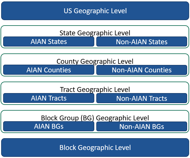
Figure 1. The AIAN spine, shown without the optional tract group geographic level between the tract and county geographic levels. This spine uses the standard census spine as a starting point and includes an AIAN branch. The optimized spine uses the AIAN spine as a starting point and redefines block groups as optimized block groups.

This document describes several optimization heuristics that perform updates on the AIAN spine to enhance specific features of the spine. We call the resulting geographic spine the optimized spine. First, the spine optimization methods redefine block groups and/or tract groups to bring a user specified set of off-spine entities (OSEs) closer to the spine and to ensure fan-out values are not too high. The definition of OSEs used in the 2020 Census production runs are described in Section 6. Second, the spine optimization algorithm reduces the variance of the final estimate by ensuring that fan-out values of the spine are also not too low, using a heuristic based on the variance matrix of the weighted least squares (WLS) estimator. For example, in cases in which a parent geounit has only one child geounit, this decision rule results in bypassing the parent geounit, i.e., reallocating all of the privacy-loss budget (PLB) from the parent to the child and then removing the parent geounit from the spine. Since the consistency-with-parent constraints in TDA require that the count estimates of the child are equal to those of the parent in cases in which a parent geounit has only one child geounit, bypassing the parent geounit in this way reduces the variance of the primitive DP answers used to derive the final histogram estimate.

The heuristics used in these optimization routines are based on existing results from the DP literature, which are provided in Section 2. Section 3 describes how geographic spines are represented here using matrices and summarizes the remainder of the paper. The method used in the first stage is described Section 4. Section 5 describes the method used in the second stage and provides a result on the privacy guarantees of the TDA when an optimized spine is used. Section 6 describes the settings related to the geographic spine that were used in the 2020 production settings runs. The next subsection outlines the notation used throughout this paper.

1.1. Notation

Throughout the paper we denote matrices using capitalized font, and vectors using lower case bold font. We denote the Kronecker product of real matrices $A,B$ by $A\otimes B,$ and elementwise division, when these matrices are conformable, by $A\oslash B$ respectively. We denote the elementwise absolute value of the real matrix $A$ by $\lvert A\rvert.$ A length $N$ column vector with each element equal to $c\in\mathbb{R}^{1}$ is denoted by $\boldsymbol{c}_{N},$ and, when there is little risk of confusion, we omit the subscript $N.$ Given two datasets (possibly with unequal numbers of rows) $x,x^{\prime},$ let $d_{\mathcal{H}}(x,x^{\prime})$ denote the minimum number of set addition and subtraction operations required to make these datasets equal.

We make use of several probability distributions, but two are worth pointing out explicitly, as their definitions are less standard. First, let the discrete Gaussian random variable be defined so that its probability mass function, $f:\mathbb{Z}\rightarrow\mathbb{R},$ is given by $f(x)\propto\exp(-(x-\mu)^{2}/(2\sigma^{2})),$ and denote the distribution of this random variable by $\textup{N}_{\mathbb{Z}}(\mu,\sigma^{2});$ see for example, [3]. Second, we also define the discrete Laplace random variable so that its probability mass function, $f:\mathbb{Z}\rightarrow\mathbb{R},$ is given by $f(x)\propto\exp(-\lvert x-\mu\rvert/b),$ and denote the distribution of this random variable by $\textup{Laplace}_{\mathbb{Z}}(\mu,\sigma^{2});$ see for example, [7]. We also conform with the usual notation for the (continuous) Gaussian distribution and denote the distributions of length $n$ column vectors with elements that are independently distributed as $\textup{N}_{\mathbb{Z}}(\boldsymbol{\mu}_{i},\boldsymbol{c}_{i})$, $\textup{Laplace}(\boldsymbol{\mu}_{i},\boldsymbol{c}_{i})$, and $\textup{Laplace}_{\mathbb{Z}}(\boldsymbol{\mu}_{i},\boldsymbol{c}_{i}),$ where $\boldsymbol{\mu}\in\mathbb{R}^{n}$ and $\boldsymbol{c}\in\mathbb{R}^{n}_{+},$ by $\textup{N}_{\mathbb{Z}}(\boldsymbol{\mu},\textup{diag}(\boldsymbol{c})),$ $\textup{Laplace}(\boldsymbol{\mu},\textup{diag}(\boldsymbol{c})),$ and $\textup{Laplace}_{\mathbb{Z}}(\boldsymbol{\mu},\textup{diag}(\boldsymbol{c}))$ respectively.

2. Differential Privacy

2.1. Privacy Definitions

The definitions of differential privacy is provided by [5, 6], and this definition is also restated below. Both definitions can be viewed as a bound on the difference between the distribution of a mechanism’s output when the input is a given database and the distribution of the output when the input is a neighboring database. The specific notion of difference used in these definitions, along with their required upper bounds, is generally self evident, but more care is required for the notion of a neighboring database because there are multiple definitions for this term that are commonly used. For example, two databases are said to be unbounded neighbors if one database can be derived by adding or removing a record from the other database; likewise, two databases are said to be bounded neighbors if one database can be derived from the other by adding one record and removing one record [10]. In other words, the set of bounded neighbors can be written as $\{x,x^{\prime}\in\mathcal{X}^{d}\mid d_{\mathcal{H}}(x,x^{\prime})=2\},$ where $\mathcal{X}^{d}$ is the set of databases with $d$ records, and the set of unbounded neighbors as $\{x,x^{\prime}\mid d_{\mathcal{H}}(x,x^{\prime})=1\}.$

The definition of neighbor has important implications because the upper bounds provided in the privacy guarantees below can be translated into an upper bound on the power of any statistical test with a given significance level of the null hypothesis that the input database is $x$ versus the alternative that it is a neighbor of $x$ [4, 13]. For example, using bounded neighbors does not provide a theoretical bound on the accuracy of inferences on the number of records in the input database. However, in the case of tests with a null hypothesis that the database is $x$ and an alternative hypothesis that it is a given bounded neighbor of $x,$ formal privacy definitions that use bounded neighbors provide stronger limitations on the accuracy of privacy attackers’ inferences. This can be shown for the privacy definitions below using the fact that a bounded neighbor of a given database is also an “unbounded neighbor of an unbounded neighbor” of the database.

The privacy guarantees provided by the TDA use a unique definition of neighbor that does not protect against certain inferences. Specifically, TDA does not protect each state’s total population or the locations of each group quarter type. In other words, TDA outputs a database with state total populations that are identical to those of the input database, and, since the frame of a U.S. decennial census excludes addresses that are unoccupied group quarters, at least one person must reside in each group quarter that appears in the census, The population residing in each group quarter type in a given geounit is constrained to be at least the number of group quarters of that type within the geounit. For more detail on these two categories of data-dependent constraints imposed by TDA, as well as those that are data-independent, see [1].

For this reason, in the context of the TDA, two databases are said to be neighbors if one database can be derived from the other by adding one record to a given state and then removing one record from that same state, such that both databases also satisfy the group quarters invariant constraints and the imputation and edit constraints of the input database of TDA. To emphasize this definition of neighbors in the presence of invariant constraints in our privacy definitions below, we define the set of pairs of neighboring databases as $\{x,x^{\prime}\in\mathcal{U}\mid d_{\mathcal{H}}(x,x^{\prime})=2\},$ where $\mathcal{U}$ is a given universal set of databases. For example, this notation is a generalization of the definition of bounded neighbors, which used $\mathcal{U}=\mathcal{X}^{\boldsymbol{d}}.$ In the results throughout this paper that use these privacy definitions, we denote the set of databases that satisfy these group quarter invariant constraints as well as the imputation and edit constraints of the confidential input data as $\mathcal{G}$ and the set of databases with $\boldsymbol{d}_{i}$ records in each state $i$ as $\mathcal{X}^{\boldsymbol{d}}.$ Using this notation, the definition of neighbors used by the TDA can be written as, $\{x,x^{\prime}\in\mathcal{X}^{\boldsymbol{d}}\cap\mathcal{G}\mid d_{\mathcal{H}}(x,x^{\prime})=2\}.$

Definition 1.

(Differential Privacy [6]) A randomized algorithm $\mathcal{M}:\mathcal{U}\rightarrow\mathcal{Y}$ satisfies $\epsilon$–differential privacy if, for all $(x,x^{\prime})\in\{x,x^{\prime}\in\mathcal{U}\mid d_{\mathcal{H}}(x,x^{\prime})=2\}$ and all $E\subset\mathcal{Y},$ we have $\textup{P}(\mathcal{M}(x)\in E)\leq\exp(\epsilon)\textup{P}(\mathcal{M}(x^{\prime})\in E).$

The definition of $\rho$–zero-Concentrated DP ($\rho$–zCDP) [2] is provided below; the DAS team uses this privacy framework for PLB accounting. Kifer et al. [9] provide more information on privacy semantic statements that can be made for DAS.

Definition 2.

(Zero-Concentrated Differential Privacy (zCDP) [2]) A randomized mechanism $\mathcal{M}:\mathcal{U}\rightarrow\mathcal{Y}$ is $\rho$–zero-concentrated differentially private ($\rho$–zCDP) if, for all $x,x^{\prime}\in\{x,x^{\prime}\in\mathcal{U}\mid d_{\mathcal{H}}(x,x^{\prime})=2\},$ all $\alpha\in(1,\infty)$, and all events $E\subset\mathcal{Y},$

$$D_{\alpha}(\mathcal{M}(x)||\mathcal{M}(x^{\prime}))\leq\rho\alpha,$$

where $D_{\alpha}(P||Q)=\log\left(\sum_{E\in\mathcal{Y}}P(E)^{\alpha}Q(E)^{(1-\alpha)}\right)/(\alpha-1)$ is the Rényi divergence of order $\alpha$ between the distributions $P$ and $Q$.

2.2. Privacy-Loss Accounting Results

A general pattern in our proofs that TDA is DP for various spine settings is to first establish that the DP primitive mechanism for each query $i$ is either $\epsilon_{i}$–DP or $\rho_{i}$–zCDP, and then use parallel and sequential composition to show that the combination of all of the DP primitive query answers used in the TDA are $\sum_{i}\epsilon_{i}$–DP or $\sum_{i}\rho_{i}$–zCDP. This section contains these intermediate results that are used in these proofs. The first two results are used in the next subsection to show that each DP primitive mechanism satisfies $\epsilon$–DP or $\rho$–zCDP.

Lemma 1.

(Theorem 3.2 [7]) Let $\Delta,\epsilon>0$. Let $q:\mathcal{U}\rightarrow\mathbb{Z}$ satisfy $|q(x)-q(x^{\prime})|\leq\Delta$ for all $x,x^{\prime}\in\{x,x^{\prime}\in\mathcal{U}\mid d_{\mathcal{H}}(x,x^{\prime})=2\}.$ Define a randomized algorithm by $\mathcal{M}(x)=q(x)+Y$ where either $Y\sim\textup{Laplace}_{\mathbb{Z}}(0,\Delta/\epsilon)$ or $Y\sim\textup{Laplace}(0,\Delta/\epsilon).$ Then $\mathcal{M}$ satisfies $\epsilon$–DP.

Lemma 2.

(Theorem 4 [3]) Let $\Delta,\epsilon>0$. Let $q:\mathcal{U}\rightarrow\mathbb{Z}$ satisfy $|q(x)-q(x^{\prime})|\leq\Delta$ for all $x,x^{\prime}\in\{x,x^{\prime}\in\mathcal{U}\mid d_{\mathcal{H}}(x,x^{\prime})=2\}.$ Define a randomized algorithm by $\mathcal{M}(x)=q(x)+Y$ where either $Y\sim\textup{N}_{\mathbb{Z}}(0,\Delta^{2}/(2\rho))$ or $Y\sim\textup{N}(0,\Delta^{2}/(2\rho)).$ Then $\mathcal{M}$ satisfies $\rho$–zCDP.

While providing a comprehensive compilation of the properties that are implied by a mechanism satisfying either $\epsilon$–DP or $\rho$–zCDP is beyond the scope of this paper, a few of these properties are worth explicitly pointing out. First, these privacy guarantees share the property that they are invariant to post-processing. In other words, if $\mathcal{M}:\mathcal{U}\rightarrow\mathcal{Y}$ satisfies either of these privacy guarantees, then so does the mechanism $f\circ\mathcal{M},$ where $f:\mathcal{Y}\rightarrow\mathcal{Z}.$ Second, if $\mathcal{M}_{1}(x)$ is $\epsilon_{1}$–DP (respectively, $\rho_{1}$–zCDP) and $\mathcal{M}_{2}(x)$ is $\epsilon_{2}$–DP ($\rho_{2}$–zCDP) then releasing the output of $\mathcal{M}_{1}(x)$ and $\mathcal{M}_{2}(x)$ simultaneously is itself $(\epsilon_{1}+\epsilon_{2})$–DP ($(\rho_{1}+\rho_{2})$–zCDP), which is called sequential composition. In some cases in which $\mathcal{M}_{1}(x)$ and $\mathcal{M}_{2}(x)$ only depend on disjoint subsets of the arbitrary dataset $x\in\mathcal{U},$ releasing the outputs of both of these mechanisms simultaneously is $(\max\;\{\epsilon_{1},\epsilon_{2}\})$–DP (respectively, $(\max\;\{\rho_{1},\rho_{2}\})$–zCDP), which is known as parallel composition. The following lemma uses sequential and parallel composition to provide privacy guarantees for a mechanism that is defined by multiple univariate mechanisms described in Lemmas 1 and 2.

Lemma 3.

(Theorem 14 [3], Proposition 1 [5], Theorem 3.2 [7]) Suppose $x,x^{\prime}\in\mathcal{X}^{d}$ differ on a single entry, and let a randomized algorithm $\mathcal{M}:\mathcal{X}^{d}\rightarrow\mathcal{Y}^{m}$ be defined by $\mathcal{M}(x)=q(x)+\boldsymbol{y}$ where $q:\mathcal{X}^{d}\rightarrow\mathcal{Y}^{m}$ and $\boldsymbol{y}$ is an $m$ dimensional column vector of independent random variables. Then we have the following.

1. Let $b_{1},\dots,b_{m}>0,$ $\epsilon>0,$ and $\sum_{j=1}^{m}\frac{\lvert q_{j}(x)-q_{j}(x^{\prime})\rvert}{b_{j}}\leq\epsilon.$ If, for all $j\in\{1,\dots,m\},$ either $\boldsymbol{y}_{j}\sim\textup{Laplace}_{\mathbb{Z}}(0,b_{j})$ or $\boldsymbol{y}_{j}\sim\textup{Laplace}(0,b_{j}),$ then $\mathcal{M}$ satisfies $\epsilon$–DP.

2. Let $\sigma_{1},\dots,\sigma_{m}>0,$ $\rho>0,$ and $\sum_{j=1}^{m}\frac{(q_{j}(x)-q_{j}(x^{\prime}))^{2}}{\sigma^{2}_{j}}\leq 2\rho.$ If, for all $j\in\{1,\dots,m\},$ either $\boldsymbol{y}_{j}\sim\textup{N}_{\mathbb{Z}}(0,\sigma^{2}_{j})$ or $\boldsymbol{y}_{j}\sim\textup{N}(0,\sigma^{2}_{j}),$ then $M$ satisfies $\rho$–zCDP.

2.3. Linear Queries and Marginal Query Groups

The notation for each query $q(\cdot)$ in the preceding subsections is more general than required to describe the TDA. Specifically, the TDA uses only linear queries. We define a linear query as a length $n$ vector, and a linear query answer as the inner product of a linear query and the histogram cell counts vector. Since we only consider linear queries from this point forward, we sometimes refer to a linear query simply as a query below. A query matrix refers to linear queries that are vertically stacked on top of one another.

All elements of the linear queries used within the TDA have elements that are either zero or one, and they are defined so that each linear query answer provides an individual count for a marginal of the full histogram. It is convenient to group the queries providing counts for the same marginal together, so we will define a query group as the linear queries that provide counts for the same marginal, vertically stacked on top of one another. For example, suppose the schema of the original database is CENRACE $\times$ HISPANIC $\times$ VOTINGAGE, where CENRACE, HISPANIC, and VOTINGAGE indicate one of 63 census race combination categories, one of two ethnicity categories, and one of two age categories, respectively. In this case, the CENRACE $\times$ VOTINGAGE query group is defined as the matrix

$$Q=I_{63}\otimes\boldsymbol{1}^{\top}_{2}\otimes I_{2},$$

and right multiplying $Q$ by the vector of histogram cell counts of a database provides the CENRACE $\times$ VOTINGAGE query group answers. More generally, the query matrix of a given query group is defined as a matrix that can be written as a series of Kronecker products of identity matrices and row vectors of ones. Note that this definition encompasses cases in which each of these Kronecker factors are all either row vectors of ones or are all identity matrices.

One of the inputs of the TDA are either the proportions of PLB, when pure DP primitive mechanisms are used, or proportions of $\rho,$ when zCDP primitive mechanisms are used, to allocate to each query for a given geolevel. The following lemma uses this notational convention, while only considering either a single geounit, to provide the $\epsilon$–DP and $\rho$–zCDP privacy guarantees of releasing the output of the primitive mechanisms of this geounit. This is used in the next section to provide the privacy guarantees of the TDA when either the conventional spine or the AIAN spine is used. Note that this lemma also makes use of a notational convention that we use throughout the rest of the paper; the histogram of detailed cell counts computed on the confidential dataset $x\in\mathcal{X}^{d}$ is denoted by $\boldsymbol{x}.$

Lemma 4.

If each $Q[i]\in\{Q[i]\}_{i=1}^{q}$ is a query group of dimension $m[i]\times n$ and the mechanism $\mathcal{M}(\boldsymbol{x}),$ outputs $\{Q[i]\boldsymbol{x}+\boldsymbol{y[i]}\}_{i=1}^{q},$ where $\boldsymbol{x}$ is a vector of the histogram counts for $x\in\mathcal{X}^{d},$ and $\boldsymbol{y[i]}$ is a length $m[i]$ column vector of independent random variables, then we have the following.

1. If, for each $i\in\{1,\dots,q\},$ either

   $\boldsymbol{y[i]}\sim\textup{Laplace}(0,\textup{diag}(\mathbf{2}_{m[i]}/(\epsilon\alpha[i])))$ or $\boldsymbol{y[i]}\sim\textup{Laplace}_{\mathbb{Z}}(0,\textup{diag}(\mathbf{2}_{m[i]}/(\epsilon\alpha[i]))),$

   where $\sum_{i}\alpha[i]=1,$ then $\mathcal{M}(\cdot)$ satisfies $\epsilon$–DP.

2. If, for each $i\in\{1,\dots,q\},$ either

   $\boldsymbol{y[i]}\sim\textup{N}(0,\textup{diag}(\mathbf{1}_{m[i]}/(\rho\alpha[i])))$ or $\boldsymbol{y[i]}\sim\textup{N}_{\mathbb{Z}}(0,\textup{diag}(\mathbf{1}_{m[i]}/(\rho\alpha[i]))),$

   where $\sum_{i}\alpha[i]=1,$ then $\mathcal{M}(\cdot)$ satisfies $\rho$–zCDP.

Proof.

Since, for each $i\in\{1,\dots,q\},$ only one element of each column of $Q[i]$ is nonzero, we use Lemma 3 to leverage parallel composition to prove both cases. This reduces the problem to carrying out sequential composition of the set of mechanisms, $\{\mathcal{M}[i](\boldsymbol{x})\}_{i}^{q},$ where $\mathcal{M}[i](\boldsymbol{x}):=Q[i]\boldsymbol{x}+\boldsymbol{y[i]}.$ In both cases, we use the fact that $\lvert Q[i]\boldsymbol{x}-Q[i]\boldsymbol{x}^{\prime}\rvert,$ where $\boldsymbol{x},\boldsymbol{x}^{\prime}$ are vectors of histogram cell counts of databases differing on a single entry, is a vector with at most two elements that are equal to one, with the remaining elements equal to zero.

In the first case, since $\sum_{j}\lvert Q[i]_{j,\cdot}\boldsymbol{x}-Q[i]_{j,\cdot}\boldsymbol{x}^{\prime}\rvert\leq 2,$ the first case in Lemma 3 implies $\mathcal{M}[i](\boldsymbol{x})$ is $\alpha[i]\epsilon$–DP. Thus, using sequential composition, releasing the output of $\{\mathcal{M}[i](\boldsymbol{x})\}_{i}$ is $\sum_{i}\alpha[i]\epsilon=\epsilon$–DP.

In the second case, since $\sum_{j}\lvert Q[i]_{j,\cdot}\boldsymbol{x}-Q[i]_{j,\cdot}\boldsymbol{x}^{\prime}\rvert^{2}\leq 2,$ the second case in Lemma 3 implies $\mathcal{M}[i](\boldsymbol{x})$ is $\alpha[i]\rho$–zCDP. Thus, using sequential composition, releasing the output of $\{\mathcal{M}[i](\boldsymbol{x})\}_{i}$ is $\sum_{i}\alpha[i]\rho=\rho$–zCDP. ∎

2.4. The Matrix Mechanism

This section describes a class of random mechanisms known as matrix mechanisms in the context of linear queries composed of query groups [11]. Using the notation introduced in Lemma 4, we assume that each of the errors of the $i^{\textup{th}}$ query group are random variables that are distributed as either $\boldsymbol{y[i]}_{j}\sim\textup{Laplace}(0,2/(\epsilon\alpha[i])),$ in the case of $\epsilon$–DP, or $\boldsymbol{y[i]}_{j}\sim\textup{N}(0,1/(\rho\alpha[i])),$ in the case of $\rho$–zCDP, for every $j\in\{1,\dots,m[i]\},$ where $\alpha[i]\in\mathbb{R}_{++}$ satisfies $\sum_{i}\alpha[i]=1.$ Also, let the workload matrix $W\in\mathbb{R}^{m\times n}$ be defined as $W:=\textup{stack}(\{Q[i]\}_{i=1}^{q}),$ the errors vector as $\boldsymbol{y}:=\textup{stack}(\{\boldsymbol{y[i]}\}_{i}^{q}),$ the PLB proportions vector as $\boldsymbol{\alpha}:=\textup{stack}(\{\boldsymbol{\alpha[i]}_{m[i]}\}_{i=1}^{q}),$ and the response variable as $\boldsymbol{z}:=W\boldsymbol{x}+\boldsymbol{y},$ which is also the vertically stacked output of the mechanism described in Lemma 4. We assume that $W$ has full column rank, which can be ensured by including the detailed cell query group in $W,$ i.e., the identity matrix.

For both of the distributions that we consider in this section, we define an alternative response variable that is observationally equivalent to $\boldsymbol{z},$ but with homoscedastic errors. For example, in the case of $\epsilon$–DP, we have $\boldsymbol{y}\sim\textup{Laplace}(0,\textup{diag}(\boldsymbol{2}\oslash(\epsilon\boldsymbol{\alpha}))),$ so we can define the rescaled errors as $\tilde{\boldsymbol{y}}:=\textup{diag}(\epsilon\boldsymbol{\alpha}/2)\boldsymbol{y},$ which are distributed as $\tilde{\boldsymbol{y}}\sim\textup{Laplace}(0,I),$ the rescaled workload as $\widetilde{W}:=\textup{diag}(\epsilon\boldsymbol{\alpha}/2)W,$ and the rescaled response variable as $\tilde{\boldsymbol{z}}:=\textup{diag}(\epsilon\boldsymbol{\alpha}/2)\boldsymbol{z}=\widetilde{W}\boldsymbol{x}+\tilde{\boldsymbol{y}}.$ In the case of $\rho$–DP, we have $\boldsymbol{y}\sim\textup{N}(0,\textup{diag}(\boldsymbol{1}\oslash(\rho\boldsymbol{\alpha}))),$ so we can define the rescaled errors as $\tilde{\boldsymbol{y}}:=\textup{diag}(\sqrt{\rho\boldsymbol{\alpha}})\boldsymbol{y},$ which are distributed as $\tilde{\boldsymbol{y}}\sim\textup{N}(0,I),$ the rescaled workload as $\widetilde{W}:=\textup{diag}(\sqrt{\rho\boldsymbol{\alpha}})W,$ and the rescaled response variable as $\tilde{\boldsymbol{z}}:=\textup{diag}(\sqrt{\rho\boldsymbol{\alpha}})\boldsymbol{z}=\widetilde{W}\boldsymbol{x}+\tilde{\boldsymbol{y}}.$

One simple example of a matrix mechanism is a mechanism that releases the weighted least squares estimates of $W\boldsymbol{x}.$ Specifically, this can be done by first estimating $\boldsymbol{x}$ as $\boldsymbol{\hat{x}}:=\operatorname*{arg\,min}_{\boldsymbol{x}}\lVert\widetilde{W}\boldsymbol{x}-\tilde{\boldsymbol{z}}\rVert^{2}_{2}=(\widetilde{W}^{\top}\widetilde{W})^{-1}\widetilde{W}^{\top}\tilde{\boldsymbol{z}},$ and then defining the output of the mechanism as $W\boldsymbol{\hat{x}}.$ Note that in either the case of $\epsilon$–DP or $\rho$–zCDP, the privacy guarantee of the final mechanism follows from the fact that a mechanism that released $\tilde{\boldsymbol{z}}$ would satisfy the same privacy guarantee, along with the invariance to post-processing property.

This simple mechanism can be generalized by making a distinction between the linear query answers provided as output and the linear queries used to estimate $\boldsymbol{\hat{x}}.$ Specifically, we define the strategy matrix $A\in\mathbb{R}^{p\times n}$ by $A:=\textup{stack}(\{R[i]\}_{i}^{r}),$ and the query group PLB proportions by $\{\gamma[i]\}_{i}^{r}.$ In the same manner as described above for $W,$ we define the rescaled strategy matrix as $\widetilde{A}:=\textup{diag}(\epsilon\boldsymbol{\gamma}/2)A,$ when deriving an $\epsilon$–DP mechanism, or $\widetilde{A}:=\textup{diag}(\sqrt{\rho\boldsymbol{\gamma}})A,$ when deriving a $\rho$–zCDP mechanism. Likewise, the rescaled error vector and response variable are defined as above so that $\tilde{\boldsymbol{z}}:=\widetilde{A}\boldsymbol{x}+\tilde{\boldsymbol{y}}.$ The final output of this matrix mechanism is then given by this alternative estimate of the linear queries in the workload $W,$ which are $W\boldsymbol{\hat{x}}=W(\widetilde{A}^{\top}\widetilde{A})^{-1}\widetilde{A}^{\top}\tilde{\boldsymbol{z}}.$

Note that the variance matrix of this output vector is given by,

$$\textup{Var}(W\boldsymbol{\hat{x}})=W(\widetilde{A}^{\top}\widetilde{A})^{-1}W^{\top}.$$

Prior research focused on using this variance matrix to find strategies that provide a low expected sum of squared errors, which is given by $\textup{Trace}(\textup{Var}(W\boldsymbol{\hat{x}}))=\textup{Trace}(W^{\top}W(\widetilde{A}^{\top}\widetilde{A})^{-1});$ see for example, [11, 12]. We use an alternative approach to motivate the heuristic used to bypass geounits in Section 5, after introducing how we represent the spine using matrices in the next section.

3. Representing Linear Queries on the Spine

In this section we describe how we represent the workload and the strategy matrices that include the linear queries for each geounit on the spine. To do so, we first consider the case in which the same query groups are used in all such geounits, and generalize this notation afterward to the case where the query matrix is dependent on the geolevel.

Let the workload of the linear queries for each geounit be denoted by $W\in\mathbb{R}^{m\times n},$ where $W=\textup{stack}(\{Q[i]\}_{i}^{q})$ and each $Q[i]$ is a query group matrix. We assign an integer to each block geounit for the purpose of ordering the blocks. Specifically, suppose that the blocks are ordered lexicographically so that blocks in the same state are adjacent to one another, within each state, blocks in the same county are adjacent, etc. For example, in the case of the conventional geographic spine, this can be achieved by sorting the blocks by their 15 digit census GEOID, as the format of the GEOID is [2 digit state FIPS code][3 digit county FIPS code][6 digit census tract code][4 digit census block code]. We refer to geounit $u\in\{1,\dots,U[l]\}$ in geolevel $l\in\{1,\dots,L\}$ as geounit $(l,u).$

Now let $b[l,u]$ denote the number of block level descendants of geounit $(l,u).$ For example, since all census blocks are descendants of the US geounit, there is a total of $b[1,1]$ blocks. Let $\boldsymbol{x}\in\mathbb{Z}^{nb[1,1]}_{+}$ be a vector of histogram cell counts over all blocks in the US, ordered in the manner described in the preceding paragraph, which we refer to as the confidential histogram cell counts below. Using this notation, we can express the query answers to the query matrix $W$ for the US geounit in terms of these block-level cell counts as $(\mathbf{1}^{\top}_{b[1,1]}\otimes W)\boldsymbol{x}.$ Likewise, the query answers for all block geounits is $(I_{b[1,1]}\otimes W)\boldsymbol{x}.$ More generally, this notation allows us to express the workload over all geolevels as sums of block-level cell counts. Specifically, a possible workload is

$$V:=B\otimes W\in\mathbb{R}^{M\times N}_{+},$$

where $M:=m\sum_{l}U[l],$ $N:=nb[1,1],$ and,

$$B:=\left[\begin{array}[]{c}B[1]\\ B[2]\\ \vdots\\ B[L-1]\\ B[L]\end{array}\right]=\left[\begin{array}[]{c}\boldsymbol{1}_{b[1,1]}^{\top}\\ \textup{block\_diag}(\{\boldsymbol{1}_{b[2,u]}^{\top}\}_{u=1}^{U[2]})\\ \vdots\\ \textup{block\_diag}(\{\boldsymbol{1}_{b[L-1,u]}^{\top}\}_{u=1}^{U[L-1]})\\ I_{b[1,1]}\end{array}\right].$$ (11)

As a summary of this notation, an example of $B\otimes W$ is shown in Figure 2.

While we use this definition for the workload over all geolevels when describing a heuristic used in the spine optimization routines below, it is not quite general enough to capture all possible workloads that a user may specify in the TDA. This is because the TDA also allows users to specify distinct strategy matrices in each geolevel, but the notation above assumes that the strategy matrix in each geolevel is $W.$ For this reason, we also use an alternative definition for the strategy matrix that is general enough to encompass all possible workloads used by TDA in our results that establish privacy guarantees. To do so, let $W[l]\in\{W[l]\}_{l=1}^{L}$ denote the workload in geolevel $l.$ Using this notation, the workload used within the TDA can be defined as,

$$V:=\left[\begin{array}[]{c}B[1]\otimes W[1]\\ B[2]\otimes W[2]\\ \vdots\\ B[L-1]\otimes W[L-1]\\ B[L]\otimes W[L]\end{array}\right].$$ (17)

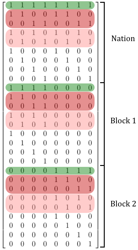
Figure 2. An example of $B\otimes W$ is given above. In this example, $B$ is given by $\textup{stack}(\mathbf{1}_{2}^{\top},I_{2}),$ which corresponds to the case in which there is one US geounit with two block geolevel child geounits. Each geounit contains a $2\times 2$ histogram, and the linear queries in $W$ are given by a total sum query ($\mathbf{1}_{2}^{\top}\otimes\mathbf{1}^{\top}_{2}$), the marginal query groups for each attribute ($I_{2}\otimes\mathbf{1}_{2}^{\top}$ and $\mathbf{1}_{2}^{\top}\otimes I_{2}$), and the detailed cell query group ($I_{2}\otimes I_{2}$). For each of the geounits, the total sum query is highlighted in green, the marginal query groups are highlighted in light and dark red, and the detailed cell query group is unhighlighted.

The following theorem uses the notation above to show that the TDA is either $\epsilon$–DP or $\rho$–zCDP, depending on whether a pure DP or zCDP framework and implementing mechanism is used, when either the conventional spine or the AIAN spine is used. The fact that geounits can be bypassed in the case of the optimized spine requires some modifications to this proof, which are described in Section 5. Note that, as in the proof below, the TDA takes the positive values in the set $\{\beta[l]\}_{l=1}^{L}$ as input, which define the PLB proportions for each geolevel.

For either the conventional spine or the AIAN spine, there is no distinction between the workload matrix and the strategy matrix, as the TDA does not alter the per-geounit workloads $\{W[l]\}_{l},$ or the matrix representation of the spine $B,$ in these cases prior to calling the implementing mechanisms.

Theorem 1.

Suppose the implementing mechanism $\mathcal{M}(\boldsymbol{x})$ outputs $\{(B[l]\otimes W[l])\boldsymbol{x}+\boldsymbol{y[l]}\}_{l=1}^{L},$ where each $W[l]$ is defined by vertically stacking the query group matrices $\{Q[i,l]\}_{i=1}^{q[l]}$ with $Q[i,l]$ of dimension $m[i,l]\times n,$ $\boldsymbol{x}$ is the confidential histogram cell counts, and $\boldsymbol{y[l]}$ is a vector of independent random variables.

Also, let $\{\beta[l]\}_{l=1}^{L}$ be defined so that $\beta[l]\in\mathbb{R}_{++}$ and $\sum_{l}\beta[l].$ Likewise, for each geolevel $l\in\{1,\dots,L\},$ let each $\alpha[i,l]\in\{\alpha[i,l]\}_{i=1}^{q[l]},$ be defined so that $\alpha[i,l]\in\mathbb{R}_{++}$ and $\sum_{i}\alpha[i,l]=1,$ and let $\boldsymbol{\alpha[l]}:=\textup{stack}(\{\boldsymbol{\alpha[i,l]}_{m[i,l]}\}_{i}).$ Then we have the following.

1. If either

   $\boldsymbol{y[l]}\sim\textup{Laplace}(\mathbf{0},\textup{diag}(\mathbf{2}\oslash(\epsilon\beta[l]\boldsymbol{\alpha[l]})))$ or $\boldsymbol{y[l]}\sim\textup{Laplace}_{\mathbb{Z}}(\mathbf{0},\textup{diag}(\mathbf{2}\oslash(\epsilon\beta[l]\boldsymbol{\alpha[l]}))),$

   then both $\mathcal{M}(\cdot)$ and the TDA are $\epsilon$–DP with respect to the neighbor definition $\{x,x^{\prime}\in\mathcal{X}^{\boldsymbol{d}}\cap\mathcal{G}\mid d_{\mathcal{H}}(x,x^{\prime})=2\}.$

2. If either

   $\boldsymbol{y[l]}\sim\textup{N}(\mathbf{0},\textup{diag}(\mathbf{1}\oslash(\rho\beta[l]\boldsymbol{\alpha[l]})))$ or $\boldsymbol{y[l]}\sim\textup{N}_{\mathbb{Z}}(\mathbf{0},\textup{diag}(\mathbf{1}\oslash(\rho\beta[l]\boldsymbol{\alpha[l]}))),$

   then both $\mathcal{M}(\cdot)$ and the TDA are $\rho$–zCDP with respect to the neighbor definition $\{x,x^{\prime}\in\mathcal{X}^{\boldsymbol{d}}\cap\mathcal{G}\mid d_{\mathcal{H}}(x,x^{\prime})=2\}.$

Proof.

Note that for each fixed $l,$ we have

$$B[l]\otimes W[l]=B[l]\otimes\textup{stack}(\{Q[i,l]\}_{i})=\textup{stack}(\{B[l]\otimes Q[i,l]\}_{i}).$$

Since each $B[l]\otimes Q[i,l]$ satisfies the definition of a query group matrix, Lemma 4 implies that releasing the output of $\mathcal{M}_{l},$ with output defined as $(B[l]\otimes W[l])\boldsymbol{x}+\boldsymbol{y[l]}$ is $(\beta[l]\epsilon)$–DP in the first case and $(\beta[l]\rho)$–zCDP in the second case. Thus, sequential composition implies that the DP primitive mechanism $\mathcal{M}(\cdot)$ is $\sum_{l}\beta[l]\epsilon=\epsilon$–DP in the first case and $\sum_{l}\beta[l]\rho=\rho$–zCDP in the second case. Since both $\rho$–zCDP and $\epsilon$–DP guarantees are invariant to post-processing, the TDA satisfies the same privacy guarantee as the primitive mechanisms. ∎

In order to describe the spine optimization routines, we will require a distinction between the workload and the strategy matrix. Specifically, in this approach, the workload maintains the same per-geounit queries $\{W\}_{i=1}^{q}$ and the same per-geounit proportions $\{\alpha[i,l]\}_{i,l}$ as the initial inputs. However, the strategy matrix will alter the matrix representation of the spine as well as the PLB proportions allocated to each geounit. We denote the matrix representation of this alternative spine as $A=\textup{stack}(\{A[l]\}_{l}^{L}),$ which we require to satisfy the following properties. First, we constrain our attention to spines that include all blocks, so $A$ must have the same number of columns as $B,$ which is $b(1,1),$ and we require the lowest geolevel to be defined as these blocks, so $A[L]:=I_{b(1,1)}.$ Second, the spine must include a US geounit, so we have $A[1]=\mathbf{1}^{\top}_{b(1,1)}.$ Third, the spine must include the same number of geolevels and be hierarchical, so, for geolevel $l\in\{1,\dots,L-1\},$ we require each row of $A[l]$ to be equal to the sum of a subset of the rows of $A[l+1].$ Since bypassing geounits results in geounits within the same geolevel having different PLB proportions, we also use $\gamma[l,u]$ to denote the geolevel PLB proportion for each geounit $(l,u),$ and $\boldsymbol{\gamma}$ to denote a vector composed of these values, using the same lexicographic ordering of the geounits described above. We will continue to use $\{\beta[l]\}_{l}^{L}$ to denote the per-geolevel PLB proportions of the initial spine, and use $\boldsymbol{\beta}$ to denote the vector $\textup{stack}(\{\boldsymbol{\beta[l]}_{U[l]}\}_{l}^{L}).$

Using the terminology from Section 2.4, we introduce the rescaling vector $r\in\mathbb{R}^{m\sum_{l}U[l]}_{+}$ and the strategy matrix $\widetilde{S}$, for later use in Section 5, as,

$$\widetilde{S}:=\textup{diag}(r)(A\otimes W)=(\textup{diag}(\boldsymbol{\gamma})\otimes\textup{diag}(\boldsymbol{\alpha}\epsilon))(A\otimes W)=(\textup{diag}(\boldsymbol{\gamma})A)\otimes(\textup{diag}(\boldsymbol{\alpha}\epsilon)W),$$

in the case in which pure $\epsilon$–DP is implemented with the Laplace mechanism and,

$$\widetilde{S}:=\textup{diag}(r)(A\otimes W)=(\textup{diag}(\sqrt{\boldsymbol{\gamma}})\otimes\textup{diag}(\sqrt{\boldsymbol{\alpha}\rho}))(A\otimes W)=(\textup{diag}(\sqrt{\boldsymbol{\gamma}})A)\otimes(\textup{diag}(\sqrt{\boldsymbol{\alpha}\rho})W),$$

in the case in which $\rho$–zCDP is implemented with the Gaussian mechanism. Also, let the stacked DP primitive mechanism answers be defined as $\tilde{\boldsymbol{z}}:=\widetilde{S}\boldsymbol{x}+\tilde{\boldsymbol{y}},$ where $\tilde{\boldsymbol{y}}=\textup{diag}(r)\boldsymbol{y},$ $\boldsymbol{y}=\textup{stack}(\{\boldsymbol{y[l]}\}_{l=1}^{L}\}),$ and $\{\boldsymbol{y[l]}\}_{l=1}^{L}$ is defined as in the previous theorem. Then the WLS estimate for this strategy matrix can be expressed as,

$$\boldsymbol{\hat{x}}=(\widetilde{S}^{\top}\widetilde{S})^{-1}\widetilde{S}\tilde{\boldsymbol{z}},$$ (18)

and the variance matrix of the ouput of the matrix mechanism is given by,

$$\textup{Var}(V\boldsymbol{\hat{x}})=V(\widetilde{S}^{\top}\widetilde{S})^{-1}V^{\top}.$$ (19)

3.1. Summary

There are two stages of the spine optimization routines, and each is described in the next two sections. The first stage takes the AIAN spine as input and then applies a method that is described in Section 4. This section introduces the OSE distance (OSED), which, for each OSE, is defined as the minimum number of on-spine geounits that must be added or subtracted from one another in order to derive the OSE. We believe that defining geounits to minimize a function (such as the maximum or the mean) of the OSED values is a non-convex optimization problem, so Section 4 also provides a computationally efficient heuristic that reduces the OSED by redefining block groups and, when they are included on the spine, tract groups.

The output of the first stage is then updated again using a method that is described in Section 5. Specifically, this section provides a result that describes when bypassing a geounit on the spine results in every expected squared error of the matrix mechanism either decreasing or remaining unchanged. Afterward, an algorithm is provided that uses this result to motivate a decision rule for when to bypass a geounit. The use of this decision rule within the TDA should also be regarded as a heuristic for two reasons. First, the output of the TDA is not defined using weighted least squares, so this decision rule is not based on the actual variance matrix of the output of the TDA. Second, the TDA uses the random noise drawn from either of the discrete distributions, $\textup{Laplace}_{\mathbb{Z}}(0,b)$ or $\textup{N}_{\mathbb{Z}}(0,\sigma^{2}),$ rather than their continuous counterparts, $\textup{Laplace}(0,b)$ and $\textup{N}(0,\sigma^{2}),$ which are the distributions that motivate this decision rule. The TDA uses the discrete distributions $\textup{Laplace}_{\mathbb{Z}}(0,b)$ and $\textup{N}_{\mathbb{Z}}(0,\sigma^{2})$ rather than $\textup{Laplace}(0,b)$ and $\textup{N}(0,\sigma^{2})$ in part because they provide lower variance, and this same fact implies that using these distributions instead would alter the decision rule. However, this difference is primarily relevant when the PLB allocated to a particular query of a geolevel is very large. For example, even when $\sigma^{2}=1,$ using $\textup{N}_{\mathbb{Z}}(0,\sigma^{2}),$ rather than $\textup{N}(0,\sigma^{2}),$ provides a decrease in the variance of less than $3\cdot 10^{-7},$ and when $\sigma^{2}=2,$ this decrease in variance is less than $3\cdot 10^{-15}.$ For this reason, in most practical cases, this second departure from the TDA is unlikely to be as important as the first.

As described in Section 2.4, the norm in the literature on the matrix mechanism is to minimize the expected sum of squared error [11, 12]. In our independent experiments, this alternative decision rule resulted in many more geounits being bypassed, which resulted in a low expected sum of squared error objective function, but with high values for some individual expected squared errors. This problem persisted even after accounting for the disproportionate number of terms in this sum from the block-level geounits by assigning each geolevel a PLB proportion that was proportional to the inverse of the number of geounits in the geolevel. In contrast, the approach that we use in TDA is more conservative, in the sense that the input spine is only changed when doing so would either decrease or not changed the expected squared error of each query of the WLS estimate. This objective function aligns more closely with our goal when setting geolevel PLB proportions, which is to ensure that the final query estimates for each geolevel satisfies a certain accuracy criterion, which is similar to the approach taken by [14].

4. Bringing Off-Spine Entities Closer to the Spine

This section describes how to redefine block groups and tract groups to bring OSEs closer to the spine. This is done by using a heuristic based on an objective function called the off-spine entity distance (OSED), which returns the minimum number of geounits that must be added or subtracted from one another to derive an OSE. This heuristic generally results in a reduction in the variance of estimates for these geographic regions, particularly when sufficient PLB proportion is allocated to the geolevels that are being redefined.

Before defining a systematic algorithm that outputs the OSEDs for each OSE, we define some additional notation. Let the set of OSEs be denoted by $\mathcal{K},$ an arbitrary encoding of the geographic spine by $g,$ and the set of geounits that are children of geounit $u$ of geolevel $l$ by $J[l,u].$ Also, let $\{C_{k}(u)\}_{k\in\mathcal{K}},$ where $C_{k}:\mathbb{N}_{+}\rightarrow\{0,1\}$ denote a set of functions such that $C_{k}(u)=1$ when the OSE $k\in\mathcal{K}$ contains the block geounit $u$ and zero otherwise.

We begin by choosing $k\in\mathcal{K}$ and finding the OSEDs for both $k$ and its complement, which we denote by $k^{\prime},$ under the (temporary) assumption that the only geolevel is the block geolevel. In this case, each block would contribute $c[k,L,u]:=C_{k}(u)$ to the OSED of OSE $k.$ Likewise, each block would contribute $c[k^{\prime},L,u]:=1-C_{k}(u)$ to the OSED of the complement of $k.$

If the block-group geolevel is added at this point, we could compose the intersection of a single block group and $k$ in one of two ways. First, we could add all the blocks to one another that are both inside of entity $k$ and inside of the block group. This would result in the block-group $u$ contributing $\sum_{v\in J(L-1,u)}c[k,l,v]$ to the OSED of $k.$ On the other hand, we could also take all the geographic extent that the block group occupies and then subtract off the geographic region of the blocks in the complement of $k.$ This would result in this block group contributing $1+\sum_{v\in J(L-1,u)}c[k^{\prime},l,v]$ to the OSED of $k.$ Note that an additional one is added in this case because of the additional step of subtracting the complement of $k$ in the block group from the block group itself. Since OSED is defined as the minimum number of geounits that must be added or subtracted to one another to define an entity, we choose the option that results in a smaller value. Since similar derivations can be carried out for the complement of $k,$ by symmetry, we have,

$$c[k,L-1,u] :=\min\left\{\sum_{v\in J(L-1,u)}c[k,l,v],\;1+\sum_{v\in J(L-1,u)}c[k^{\prime},l,v]\right\}$$ (20)

$$c[k^{\prime},L-1,u] :=\min\left\{\sum_{v\in J(L-1,u)}c[k^{\prime},l,v],\;1+\sum_{v\in J(L-1,u)}c[k,l,v]\right\}.$$ (21)

Note that (20) and (21) provide a closed form solution for $\{(c[k,L-1,u],c[k^{\prime},L-1,u])\}_{u}$ in terms of $\{(c[k,L,u],c[k^{\prime},L,u])\}_{u}.$ Similar logic can be repeated to derive to derive the following recursive system of equations.

$$c[k,l-1,u] :=\min\left\{\sum_{v\in J(l-1,u)}c[k,l,v],\;1+\sum_{v\in J(l-1,u)}c[k^{\prime},l,v]\right\}$$ (22)

$$c[k^{\prime},l-1,u] :=\min\left\{\sum_{v\in J(l-1,u)}c[k^{\prime},l,v],\;1+\sum_{v\in J(l-1,u)}c[k,l,v]\right\}$$ (23)

Since all entities are assumed to be contained within the US, the final OSED for entity $k$ can be found by applying these recursions to the root geounit and defining this OSED as $c[k,1,1].$ Afterward, our final objective function is defined by a reduce operation, such as a function that returns the mean or maximum OSED. This computation is summarized in Algorithm 1.

for $k\in\mathcal{K}$ do

       for $u\in\textup{Geounits\_in\_Geolevel}(L,g)$ do

             $c[k,L,u]\leftarrow C_{k}(u)$

             $c[k^{\prime},L,u]\leftarrow 1-C_{k}(u)$

            

      for $l\in\{L-1,L-2,\dots,1\}$ do

             for $u\in\textup{Geounits\_in\_Geolevel}(l,g)$ do

                   $x\leftarrow\sum_{v\in\textup{Children}(u,l,g)}c[k,l+1,v]$

                   $y\leftarrow\sum_{v\in\textup{Children}(u,l,g)}c[k^{\prime},l+1,v]$

                   $c[k,l,u]\leftarrow\min\;\{x,y+1\}$

                   $c[k^{\prime},l,u]\leftarrow\min\;\{y,x+1\}$

            

      

$\mathbf{return}$ $h(\{c[k,1,1]\}_{k\in\mathcal{K}})$

Algorithm 1 OSEDs_Reduced$(g,\mathcal{K},\{C_{k}(\cdot)\}_{k},h(\cdot),L)$

In the most general setting, in which the OSEs are not necessarily disjoint, formulating an algorithm that redefines block groups and tract groups in order to minimize the OSEDs with a polynomial time complexity appears to be a difficult problem because of the similarity of this optimization problem to a covering problem. For this reason, Algorithm 2 describes a greedy approach to approximate the optimal redefinitions of tract groups in a computationally tractable manner. In contrast, block groups are redefined as optimized block groups by combining blocks within a given tract geounit, and within the same intersection of the OSEs. As described in the code below, each optimized block group is composed of up to $\sqrt{n}+\textup{fanout\_cutoff}$ blocks, where $n$ is the blocks in the optimized block group’s parent tract and fanout_cutoff is a user choice parameter. This choice is motivated by the fact that the smallest maximum fanout value among a given tract and its child geounits is $\left\lceil{\sqrt{n}}\right\rceil,$ where $\left\lceil{\cdot}\right\rceil$ denotes the ceiling function. For example, for a tract with 100 block geounit descendants, redefining its children by 10 optimized block group child geounits, each with 10 block child geounits, would result in the lowest possible maximum fanout of 10 among these 11 geounits, so the optimized block groups within this tract would contain no more than $10+\textrm{fanout\_cutoff}$ blocks in this case. Note that a similar approach is used to define the maximum number of tracts within a tract group in Algorithm 2.

Algorithm 2 uses $\boldsymbol{x}\preceq_{\textup{lexicographic}}\boldsymbol{y},$ where $\boldsymbol{x},\boldsymbol{y}\in\mathbb{R}^{n},$ to denote the lexicographic less than or equal to partial ordering, which is defined as $\bot$ when $\boldsymbol{x}\neq\boldsymbol{y}$ and the first index $i$ for which $\boldsymbol{x}_{i}$ and $\boldsymbol{y}_{i}$ differ satisfies $\boldsymbol{x}_{i}>\boldsymbol{y}_{i},$ and $\top$ otherwise.

Note that Algorithm 2 does not alter the PLB proportions of the input spine, which is the AIAN spine. The next section describes the Algorithm used to update these proportions, along with the spine that is output from Algorithm 2, in the second spine optimization stage.

// Within each tract, redefine block groups by combining groups of $\sqrt{n}+\textup{fanout\_cutoff}$ blocks in the intersections of the same OSEs, where $n$ is the number of blocks in the tract.

// Initialize tract groups so that they each have one child Tract.

current_OSEDs $\leftarrow\textup{OSEDs\_Reduced}(g,\mathcal{K},\{C_{k}(\cdot)\}_{k},\textup{Sort\_Descending}(\cdot))$

for $i\in\{1,\dots\}$ do

       $g\_\textup{changed}\leftarrow\bot$

       for $\textup{county}\in\textup{Counties}(g)$ do

             $n\leftarrow$ Number_of_tracts_in_county$($county$)$

             for $u,v\in\textup{Children}(\textup{county})$ do

                   if $\textup{Card}(\textup{Children}(u)\cup\textup{Children}(v))>\sqrt{n}+\textup{fanout\_cutoff}$ then

                         continue

                        

                  $g^{\prime}\leftarrow$ Combine_Siblings$(u,v,g)$

                   test_OSEDs $\leftarrow\textup{OSEDs\_Reduced}(g^{\prime},\mathcal{K},\{C_{k}(\cdot)\}_{k},\textup{Sort\_Descending}(\cdot))$

                   if test_OSEDs $\preceq_{\textup{lexicographic}}$ current_OSEDs then

                         $g\leftarrow g^{\prime}$

                         current_OSEDs $\leftarrow$ test_OSEDs

                         $g\_\textup{changed}\leftarrow\top$

                        

                  

            

      if $\textbf{not }g\_\textup{changed}$ then

             break

            

      

$\mathbf{return}$ $g$

Algorithm 2 Redefine_Block_Groups_and_Tract_Groups$(g,\mathcal{K},\{C_{k}(\cdot)\}_{k})$

5. A Pareto Frontier of Geounit Definitions

This section uses a matrix mechanism to provide a decision rule for when it is best to bypass a geounit. To do so, we constrain our attention to DP implementing mechanisms that use noise drawn from the continuous distributions $\textup{N}(\cdot)$ and $\textup{Laplace}(\cdot).$ We also suppose that the matrix $B$ is the matrix representation of the spine that is used as input of this method. In the case of the TDA, this spine is formed using the output of Algorithm 2.

It is also worth explicitly stating how we define the operation of bypassing a parent geounit. We define the operation of bypassing a parent geounit with $c$ children, each with equal PLB proportions, by, 1) creating $c$ geounits in the geolevel of the parent, each with a geolevel proportion given by the sum of proportion allocated to the parent and one of the children, 2) defining the single child of each of these $c$ new geounits by one of the children, 3) removing the old parent geounit, 4) redefining the geolevel proportion of each child to be zero. Thus, even though we call this operation “bypassing a parent,” this operation actually moves the geolevel PLB proportion to a higher geolevel. This ensures that this operation does not change the total number of geolevels, and since the TDA fixes the final estimates in a top-down manner, so that the consistency with parent constraints are satisfied, this also ensures that the entire share of the geolevel PLB allocations are used in cases in which a parent geounit has only one child geounit. Although this definition describes the operation used within the TDA, the decision rules developed in this section only depend on properties of $\widetilde{S}^{\top}\widetilde{S},$ and using this definition of the bypass operation impacts this matrix in the same way as simply reallocating the geolevel PLB proportion of the parent geounit to the children. For this reason, we motivate the decision rules described in this section on this simpler definition of the bypass operation.

Using the notation from 3, recall that the expected squared errors of the output of the matrix mechanism with the strategy matrix $\widetilde{S}$ are given by the diagonal of $\textup{Var}(V\boldsymbol{\hat{x}}),$ as defined in (19). The next result describes a case in which each of these expected squared errors can be decreased, or remain unchanged, by bypassing a parent. In cases in which the initial PLB proportion of a parent and its children are equal, this result implies that accuracy can be improved by bypassing the parent geounit when it has less than or equal to three child geounits. The decision rule used for the case in which $\rho$–zCDP is implemented using Gaussian mechanisms is discussed after the proof.

Theorem 2.

Suppose that $\epsilon$–DP is implemented using Laplace mechanisms and that the per-geolevel query strategies and query PLB proportions are the same in each geolevel. Also suppose that the geolevel PLB allocated to each of the $c$ children of geounit $(l,1)$ are equal (ie: $\gamma[l+1,u]=\gamma[l+1,v]$ for all $u,v\in\{1,\dots,c\}$). If $\gamma[l+1,1]\geq(c-1)\gamma[l,1]/2,$ then, for any $W$ and $\{\alpha[i]\}_{i},$ reallocating the PLB assigned to geounit $(l,1)$ to its children will either decrease or leave unchanged each of the diagonal elements of $\textup{Var}(V\boldsymbol{\hat{x}}).$

Proof.

Let $\{\gamma_{0}[l,u]\}_{l,u}$ and $\{\gamma_{1}[l,u]\}_{l,u}$ denote the geounit PLB proportions before and after reallocation, respectively. Likewise, let $\boldsymbol{\hat{x}}_{0}$ and $\boldsymbol{\hat{x}}_{1}$ denote the WLS estimate before and after reallocation, respectively. Also, for the symmetric matrices $C,D\in\mathbb{R}^{n\times n}$ we will use $C\leq D$ to denote the condition that $C-D$ is negative semidefinite and $C\leq 0$ to denote the condition that $C$ is negative semidefinite. The variance matrix of the WLS estimate before (respectively, after) bypassing geounit $(l,1)$ is proportional to,

$$\textup{Var}(\boldsymbol{\hat{x}}_{i})= ((\textup{diag}(\boldsymbol{\gamma}_{i})A\otimes W)^{\top}(\textup{diag}(\boldsymbol{\gamma}_{i})A\otimes W))^{-1}$$

$$= ((A^{\top}\textup{diag}(\boldsymbol{\gamma}_{i})\otimes W^{\top})(\textup{diag}(\boldsymbol{\gamma}_{i})A\otimes W))^{-1}$$

$$= ((A^{\top}\textup{diag}(\boldsymbol{\gamma}_{i}^{2})A)\otimes(W^{\top}W))^{-1}$$

$$= (A^{\top}\textup{diag}(\boldsymbol{\gamma}_{i}^{2})A)^{-1}\otimes(W^{\top}W)^{-1},$$

where $i=0$ (respectively, $i=1$). We prove the sufficient condition that $\textup{Var}(\boldsymbol{\hat{x}}_{1})\leq\textup{Var}(\boldsymbol{\hat{x}}_{0}).$ Given the variance matrix of the WLS estimator above, this condition is equivalent to,

$$\textup{Var}(\boldsymbol{\hat{x}}_{1})<\textup{Var}(\boldsymbol{\hat{x}}_{0})\iff$$

$$(A^{\top}\textup{diag}(\boldsymbol{\gamma}_{1}^{2})A)^{-1}\otimes(W^{\top}W)^{-1}\leq(A^{\top}\textup{diag}(\boldsymbol{\gamma}_{0}^{2})A)^{-1}\otimes(W^{\top}W)^{-1}\iff$$

$$((A^{\top}\textup{diag}(\boldsymbol{\gamma}_{1}^{2})A)^{-1}-(A^{\top}\textup{diag}(\boldsymbol{\gamma}_{0}^{2})A)^{-1})\otimes(W^{\top}W)^{-1}\leq 0.$$

Since we assume that $W^{\top}W$ is positive definite, this condition holds if and only if,

$$((A^{\top}\textup{diag}(\boldsymbol{\gamma}_{1}^{2})A)^{-1}-(A^{\top}\textup{diag}(\boldsymbol{\gamma}_{0}^{2})A)^{-1})\leq 0\iff$$

$$(A^{\top}\textup{diag}(\boldsymbol{\gamma}_{1}^{2})A)^{-1}\leq(A^{\top}\textup{diag}(\boldsymbol{\gamma}_{0}^{2})A)^{-1}\iff$$

$$A^{\top}\textup{diag}(\boldsymbol{\gamma}_{1}^{2})A\geq A^{\top}\textup{diag}(\boldsymbol{\gamma}_{0}^{2})A\iff$$

$$A^{\top}\textup{diag}(\boldsymbol{\gamma}_{1}^{2}-\boldsymbol{\gamma}_{0}^{2})A\geq 0$$

Note that the only elements of $\boldsymbol{\gamma}_{1}$ that are not equal to $\boldsymbol{\gamma}_{0}$ can be defined in terms of $\boldsymbol{\gamma}_{0}$ by $\gamma_{1}[l+1,u]=\gamma_{0}[l+1,u]+\gamma_{0}[l,1]$ for all $u\in\{1,\dots c\}$ and $\gamma_{1}[l,1]=0.$ Thus, $A^{\top}\textup{diag}(\boldsymbol{\gamma}_{0}^{2}-\boldsymbol{\gamma}_{1}^{2})A$ is a block matrix with a single block that is nonzero. Let $n[u]:=b[l+1,u]$ for $u\in\{1\dots,c\}.$ This block is of dimension $b[l,1]\times b[l,1],$ and is given by

$$D:=\gamma_{0}[l,1]\left[\begin{array}[]{cccc}2\gamma_{0}[l+1,1]\mathbf{1}_{n[1]}\mathbf{1}_{n[1]}^{\top}&-\gamma_{0}[l,1]\mathbf{1}_{n[1]}\mathbf{1}_{n[2]}^{\top}&-\gamma_{0}[l,1]\mathbf{1}_{n[1]}\mathbf{1}_{n[3]}^{\top}&\cdots\\ -\gamma_{0}[l,1]\mathbf{1}_{n[2]}\mathbf{1}_{n[1]}^{\top}&2\gamma_{0}[l+1,2]\mathbf{1}_{n[2]}\mathbf{1}_{n[2]}^{\top}&-\gamma_{0}[l,1]\mathbf{1}_{n[2]}\mathbf{1}_{n[3]}^{\top}&\\ -\gamma_{0}[l,1]\mathbf{1}_{n[3]}\mathbf{1}_{n[1]}^{\top}&-\gamma_{0}[l,1]\mathbf{1}_{n[3]}\mathbf{1}_{n[2]}^{\top}&2\gamma_{0}[l+1,3]\mathbf{1}_{n[3]}\mathbf{1}_{n[3]}^{\top}\\ \vdots&&&\ddots\\ \end{array}\right].$$

For each $i\in\{1,\dots,c\},$ let $a[i]:=\sum_{j=1}^{i-1}n[j],$ $b[i]:=\sum_{j=i+1}^{c}n[j],$ and $\boldsymbol{t_{i}}:=(\mathbf{0}_{a[i]}^{\top},\mathbf{1}_{n[i]}^{\top}/n[i],$ $\mathbf{0}_{b[i]}^{\top})^{\top}.$ Note that the matrix $D$ has only $c$ unique columns, and the vectors $\{\boldsymbol{t_{i}}\}_{i=1}^{c}$ provide an orthogonal basis for the span of these columns. Let $T:=\textup{horizontal\_stack}(\{\boldsymbol{t_{i}}\}_{i}).$ Thus,

$D\geq 0\iff TDT^{\top}\geq 0\iff$

$\left[\begin{array}[]{cccc}2\gamma_{0}[l+1,1]\gamma_{0}[l,1]&-\gamma_{0}[l,1]^{2}&-\gamma_{0}[l,1]^{2}&\cdots\\ -\gamma_{0}[l,1]^{2}&2p_{0}(l+1,2)\gamma_{0}[l,1]&-\gamma_{0}[l,1]^{2}&\\ -\gamma_{0}[l,1]^{2}&-\gamma_{0}[l,1]^{2}&2\gamma_{0}[l+1,3]\gamma_{0}[l,1]\\ \vdots&&&\ddots\\ \end{array}\right]\geq 0\iff$

D’ := diag$(\mathbf{1}_{r}(2\gamma_{0}[l+1,1]\gamma_{0}[l,1]+\gamma_{0}[l,1]^{2}))-\mathbf{1}_{r}\mathbf{1}_{r}^{\top}\gamma_{0}[l,1]^{2}\geq 0.$

Since $\gamma_{0}[l,u]\geq 0$ for all $l$ and $u,$ the eigenvector of $D^{\prime}$ corresponding to the smallest eigenvalue is $\mathbf{1}_{r},$ so this matrix is positive semidefinite when,

$2\gamma_{0}[l+1,1]\gamma_{0}[l,1]\geq(c-1)\gamma_{0}[l,1]^{2}.$

Since $(l,1)$ was not bypassed in our initial PLB allocation, $\gamma_{0}[l,1]\neq 0,$ so we have,

$\gamma_{0}[l+1,1]\geq(c-1)\gamma_{0}[l,1]/2.$

∎

Remark 1

Consider two cases in which the only query in $W$ is a total population query. First, if the parent is not bypassed, we could construct unbiased estimates of the total population of the parent by either observing the DP answer for the parent directly, which has a variance of $2/\gamma[l,1]^{2},$ or by summing the DP answers of the children together, which has a variance of $2c/\gamma[l+1,1]^{2}.$ The mean with inverse variance weighting provides the linear combination of these estimates with the lowest possible variance of $2c/(c\gamma[l,1]^{2}+\gamma[l+1,1]^{2})$ in this case. Second, if we did bypass the parent, we could estimate the total population query for the parent by summing the total population of the children, which would have a variance of $2c/(\gamma[l+1,1]+\gamma[l,1])^{2}$ in this case. The theorem above can be viewed as a statement that limiting our attention to a single total population query, and to only the parent and its children, in this way is without loss of generality, at least for the purpose of finding the cases in which bypassing the parent does not increase the expected error for any query in any geounit. This is because $2c/(c\gamma[l,1]^{2}+\gamma[l+1,1]^{2})\geq 2c/(\gamma[l+1,1]+\gamma[l,1])^{2}$ if and only if $\gamma[l+1,1]\geq(c-1)\gamma[l,1]/2,$ which is the same requirement given in the statement of the theorem. ∎

Remark 2

This theorem may be of independent interest in the DP literature because other authors have already considered strategy matrices that have a hierarchical structure that is analogous to the matrix representation of the spine $A$ above, and this result can be used to narrow the search space of the set of hierarchical strategy matrices considered when choosing a strategy matrix with this property [8, 11]. For example, when using the WLS approach described by [8] with PLB proportions that are the same for each level of the hierarchy and with the children of each non-leaf node defined by either two or three sub-intervals of the range of the parent node, this result implies that the the expected squared error of an arbitrary linear query can be reduced by increasing the number of sub-intervals used to define these child nodes. ∎

One can use a similar technique to show that, in the case in which $\rho$–zCDP implementing Gaussian mechanisms are used to define $\boldsymbol{y},$ bypassing a parent will increase at least one diagonal element of $\textup{Var}(V\boldsymbol{\hat{x}})$ whenever the parent has two or more children, and the diagonal elements of $\textup{Var}(V\boldsymbol{\hat{x}})$ will remain unchanged whenever the parent has only one child. In part for this reason, our decision rule for the case implementing $\rho$–zCDP with Gaussian mechanisms is to bypass parent geounits with only one child. However, given the top-down manner in which the TDA fixes estimates to ensure consistency with the estimates of the parent geounits, the estimates of a child geounit are fixed by those of the parent geounit whenever the parent only has one child geounit. Thus, we need not solely rely on the change in the diagonal elements of $\textup{Var}(V\boldsymbol{\hat{x}})$ to motivate the decision rule for this case; an alternative motivation is provided in the following observation. Note that the decision rule provided in Theorem 2 results in at least the same number of geounits being bypassed, since, whenever $c=1,$ the condition in the statement of the theorem becomes $\gamma[l+1,1]\geq 0,$ and we require each $\gamma[l,u]$ to be non-negative.

Observation 1.

The answers for each child geounit that does not have a sibling geounit that are provided by the DP implementing mechanism do not impact the output of TDA. Thus, the variance of the DP implementing mechanisms’ output that are actually used to construct the final estimates in the TDA can be decreased by bypassing all parent geounits with only one child.

Algorithm 3 summarizes how both decision rules are used within the spine optimization routines of the TDA. Note that this algorithm starts at the block group geolevel and iterates up the spine to the US geolevel, rather than starting at the US geolevel and moving downward, which ensures that no remaining geounits can be bypassed after only one pass through the spine.

for $l\in\{L-1,L-2,\dots,1\}$ do

       for parent in geolevel $l$ do

             $\beta$_child $\leftarrow$ $\textup{min}_{u\in\textup{Children}(\textup{parent})}\;\beta[l+1,u]$

             $\beta$_parent $\leftarrow\beta[l,\textup{parent}]$

             $c\leftarrow\textup{Card}(\textup{Children}(\textup{parent}))$

             if Pure_DP $\textup{and }\beta\_\textup{child}\geq(c-1)\beta\_\textup{parent}/2$ then

                   $B,\{\beta[l,u]\}_{l,u}\leftarrow\textup{Bypass\_Parent\_Geounit}(\textup{parent},B,\{\beta[l,u]\}_{l,u})$

            else if $c=1$ then

                   $B,\{\beta[l,u]\}_{l,u}\leftarrow\textup{Bypass\_Parent\_Geounit}(\textup{parent},B,\{\beta[l,u]\}_{l,u})$

            

      

$\mathbf{return}$ $B,\{\beta[l,u]\}_{l,u}$

Algorithm 3 Move_Spine_to_Pareto_Frontier$(B,\{\beta[l,u]\}_{l,u},\textup{pure\_DP}\in\{\top,\bot\})$

5.1. The impact of Spine Optimization on the Privacy Guarantees of TDA

Using the TDA with the spine that is output from Algorithm 2 does not alter the privacy guarantees of the TDA because the same arguments used in the proof of Theorem 1 apply to this case as well. However, the same cannot be said for the spine that is output from Algorithm 3 when at least one geounit is bypassed. The following theorem generalizes the argument used in Theorem 1 to show that using the spine output from Algorithm 3 within the TDA does not impact the privacy guarantees.

Theorem 3.

Suppose the implementing mechanism $\mathcal{M}(\boldsymbol{x})$ outputs $\{(A[l]_{u,\cdot}\otimes W[l])\boldsymbol{x}+\boldsymbol{y}[l,u]\}_{l,u},$ where each $A[l]\in\{0,1\}^{U[l]\times b[1,1]}$ is the matrix representation of geolevel $l\in\{1,\dots,L\}$ of the spine output from the spine optimization routines described in Sections 4 and 5, each $W[l]$ is defined by vertically stacking the query group matrices $\{Q[i,l]\}_{i=1}^{q[l]}$ with $Q[i,l]$ of dimension $m[i,l]\times n,$ $\boldsymbol{x}$ is the confidential histogram cell counts for dataset $x\in\mathcal{X}^{\boldsymbol{d}}\cap\mathcal{G},$ and $\boldsymbol{y[l,u]}$ is a vector of either independent random variables or has all elements equal to $\infty.$

Also, let the input geolevel PLB proportions $\{\beta[l]\}_{l}$ be defined so that $\beta[l]\in\mathbb{R}_{++}$ and $\sum_{l}\beta[l]=1,$ and let $\{\gamma[l,u]\}_{l,u}$ denote the resulting geolevel PLB proportions that is output from the spine optimization routines. Likewise, for each geolevel $l\in\{1,\dots,L\},$ let each $\alpha[i,l]\in\{\alpha[i,l]\}_{i=1}^{q[l]},$ be defined so that $\alpha[i,l]\in\mathbb{R}_{++}$ and $\sum_{i}\alpha[i,l]=1,$ and let $\boldsymbol{\alpha[l]}:=\textup{stack}(\{\boldsymbol{\alpha[i,l]}_{m[i,l]}\}_{i}).$ Then we have the following.

1. If $\boldsymbol{y[l,u]}=\infty$ when $\gamma[l,u]=0,$ and is distributed as either $\boldsymbol{y[l,u]}\sim\textup{Laplace}(\mathbf{0},\textup{diag}(\mathbf{2}\oslash(\epsilon\gamma[l,u]\boldsymbol{\alpha[l]})))$ or $\boldsymbol{y[l,u]}\sim\textup{Laplace}_{\mathbb{Z}}(\mathbf{0},\textup{diag}(\mathbf{2}\oslash(\epsilon\gamma[l,u]\boldsymbol{\alpha[l]})))$ when $\gamma[l,u]>0,$ then both $\mathcal{M}(\cdot)$ and the TDA are $\epsilon$–DP with respect to the neighbor definition $\{x,x^{\prime}\in\mathcal{X}^{\boldsymbol{d}}\cap\mathcal{G}\mid d_{\mathcal{H}}(x,x^{\prime})=2\}.$

2. If $\boldsymbol{y[l,u]}=\infty$ when $\gamma[l,u]=0,$ and is distributed as either $\boldsymbol{y[l,u]}\sim\textup{N}(\mathbf{0},\textup{diag}(\mathbf{1}\oslash(\rho\gamma[l,u]\boldsymbol{\alpha[l]})))$ or $\boldsymbol{y[l,u]}\sim\textup{N}_{\mathbb{Z}}(\mathbf{0},\textup{diag}(\mathbf{1}\oslash(\rho\gamma[l,u]\boldsymbol{\alpha[l]})))$ when $\gamma[l,u]>0,$ then both $\mathcal{M}(\cdot)$ and the TDA are $\rho$–zCDP with respect to the neighbor definition $\{x,x^{\prime}\in\mathcal{X}^{\boldsymbol{d}}\cap\mathcal{G}\mid d_{\mathcal{H}}(x,x^{\prime})=2\}.$

Proof.

For $x\in\mathcal{X}^{\boldsymbol{d}}\cap\mathcal{G},$ let the set of datasets $x^{\prime}\in\mathcal{X}^{\boldsymbol{d}}\cap\mathcal{G}$ that differ from $x$ on a single entry be denoted by $\textup{N}(x).$ Also, let $T[l]:=\{u\in\mathbb{Z}_{++}\mid u<U[l]\textup{ and }\gamma[l,u]>0\}.$ The output of all the DP implementing mechanisms is observationally equivalent to the set of finite output elements, or $\{(A[l]_{u,\cdot}\otimes W[l])\boldsymbol{x}+\boldsymbol{y}[l,u]\}_{l,u\in T[l]},$ because, independently of the data, the remaining DP mechanism answers are infinite with probability one. Thus, without loss of generality, we can restrict our attention to an alternative mechanism that outputs $\{(A[l]_{u,\cdot}\otimes W[l])\boldsymbol{x}+\boldsymbol{y}[l,u]\}_{l,u\in T[l]}.$ Let $\widehat{A[l]}:=A[l]_{T[l],\cdot},$ and $\boldsymbol{\hat{\gamma}[l]}:=\textup{stack}(\{\gamma[l,u]\}_{l,u\in T[l]}),$ so the strategy matrix for this alternative mechanism can be written as,

$$D:=\textup{stack}(\{\widehat{A}[l]\otimes W[l]\}_{l}).$$

In the case of the first result of the theorem, the noise for this mechanism is distributed as either $\hat{\boldsymbol{y}}\sim\textup{Laplace}(\mathbf{0},\textup{diag}(\boldsymbol{\hat{b}}))$ or $\hat{\boldsymbol{y}}\sim\textup{Laplace}_{\mathbb{Z}}(\mathbf{0},\textup{diag}(\boldsymbol{\hat{b}})),$ where $\boldsymbol{\hat{b}}:=\textup{stack}(\{\boldsymbol{\hat{b}}[l]\}_{l})$ and $\boldsymbol{\hat{b}}[l]:=\textbf{2}\oslash(\epsilon(\boldsymbol{\hat{\gamma}[l]}\otimes\boldsymbol{\alpha}[l])).$ Thus, we will show the following condition, which, by the first result in Lemma 3, is a sufficient condition for the result,

$$\max_{x\in\mathcal{X}^{\boldsymbol{d}}\cap\mathcal{G},\;x^{\prime}\in\textup{N}(x)}\;\sum_{i}\left|D_{i,\cdot}(\boldsymbol{x}-\boldsymbol{x}^{\prime})/\boldsymbol{\hat{b}}_{i}\right|\leq\epsilon.$$ (24)

Starting from the left hand side of this inequality, we have,

$$\max_{x\in\mathcal{X}^{\boldsymbol{d}}\cap\mathcal{G},\;x^{\prime}\in\textup{N}(x)}\;\sum_{i}\left|\left(\textup{diag}(\mathbf{1}\oslash\boldsymbol{\hat{b}})D\right)_{i,\cdot}(\boldsymbol{x}-\boldsymbol{x}^{\prime})\right|\leq 2\max_{j}\;\sum_{i}\left(\textup{diag}(\mathbf{1}\oslash\boldsymbol{\hat{b}})D\right)_{i,j}=$$

$$2\max_{j}\;\sum_{i}\textup{stack}\left(\{\textup{diag}\left(\epsilon(\boldsymbol{\hat{\gamma}[l]}\otimes\boldsymbol{\alpha}[l])/2\right)(\widehat{A}[l]\otimes W[l])\}_{l}\right)_{i,j}=$$

$$\epsilon\max_{j}\;\sum_{l}\sum_{i}\left(\textup{diag}(\boldsymbol{\hat{\gamma}[l]})\widehat{A}[l]\otimes\textup{diag}(\boldsymbol{\alpha}[l])W[l]\right)_{i,j}.$$ (25)

Note that each of the row sums of $\textup{diag}(\boldsymbol{\alpha}[l])W[l],$ i.e., the vector $W[l]^{\top}\textup{diag}(\boldsymbol{\alpha}[l])\mathbf{1}=W[l]^{\top}\boldsymbol{\alpha}[l],$ is equal to $\mathbf{1}$ because $\sum_{k}Q[i,l]_{k,\cdot}=\mathbf{1}^{\top}$ and $\sum_{k}\alpha[k,l]=1.$ Thus, since each column $j$ of $\textup{diag}(\boldsymbol{\hat{\gamma}[l]})\widehat{A}[l]$ contains at most one nonzero value, we have,

$$\epsilon\max_{j}\;\sum_{l}\sum_{i}\left((\textup{diag}(\boldsymbol{\hat{\gamma}[l]})\widehat{A}[l])\otimes(\textup{diag}(\boldsymbol{\alpha}[l])W[l])\right)_{i,j}=$$

$$\epsilon\max_{j}\;\sum_{l}\sum_{i}\left(\textup{diag}(\boldsymbol{\hat{\gamma}[l]})\widehat{A}[l]\right)_{i,j}=\epsilon\max_{j}\;\sum_{i}\left(\textup{diag}(\hat{\boldsymbol{\gamma}})\widehat{A}\right)_{i,j},$$

where $\hat{\boldsymbol{\gamma}}:=\textup{stack}(\{\boldsymbol{\hat{\gamma}[l]}\}_{l}).$ Note that $\sum_{i}\left(\textup{diag}(\hat{\boldsymbol{\gamma}})\widehat{A}\right)_{i,j}$ is equal to the sum of the geolevel PLB proportions along a path from the US geounit to the block geounit $j.$ Since the bypass operation used within Algorithm 3 does not change this sum, and its initial value is $\sum_{l}\beta[l]=1,$ we have

$$\epsilon\max_{j}\;\sum_{i}\left(\textup{diag}(\hat{\boldsymbol{\gamma}})\widehat{A}\right)_{i,j}=\epsilon\sum_{l}\beta[l]=\epsilon,$$

which implies inequality (24).

Similar logic also implies the second result of the theorem. Specifically, in this case we can use the second result of Lemma 3, and the fact that for each $x\in\mathcal{X}^{\boldsymbol{d}}\cap\mathcal{G}$ and $x^{\prime}\in\textup{N}(x)$ we have $(D_{i,\cdot}(\boldsymbol{x}-\boldsymbol{x}^{\prime}))^{2}=\left|D_{i,\cdot}(\boldsymbol{x}-\boldsymbol{x}^{\prime})\right|,$ to derive the sufficient condition,

$$\max_{x\in\mathcal{X}^{d},\;x^{\prime}\in\textup{N}(x)}\;\sum_{i}\left|D_{i,\cdot}(\boldsymbol{x}-\boldsymbol{x}^{\prime})\right|/\boldsymbol{\hat{\sigma}}_{i}^{2}\leq 2\rho,$$ (26)

where $\boldsymbol{\hat{\sigma}^{2}}:=\textup{stack}(\{\boldsymbol{\hat{\sigma}^{2}[l]}\}_{l})$ and $\boldsymbol{\hat{\sigma}^{2}[l]}:=\mathbf{1}\oslash(\rho(\boldsymbol{\hat{\gamma}[l]}\otimes\boldsymbol{\alpha[l]})).$ This inequality follows from,

$$\max_{x\in\mathcal{X}^{\boldsymbol{d}}\cap\mathcal{G},\;x^{\prime}\in\textup{N}(x)}\;\sum_{i}\left|D_{i,\cdot}(\boldsymbol{x}-\boldsymbol{x}^{\prime})\right|/\boldsymbol{\hat{\sigma}^{2}}_{i}\leq 2\max_{j}\sum_{i}\left(\textup{diag}(\mathbf{1}\oslash\boldsymbol{\hat{\sigma}^{2}})D\right)_{i,j}=$$

$$2\rho\max_{j}\sum_{i}\left(\textup{diag}(\boldsymbol{\hat{\gamma}[l]}\otimes\boldsymbol{\alpha[l]})D\right)_{i,j}.$$ (27)

Since this last value is equal to the value of (25) multiplied by $2\rho/\epsilon,$ and the logic above implies the value of (25) is equal to $\epsilon,$ we have,

$$2\rho\max_{j}\sum_{i}\left(\textup{diag}(\boldsymbol{\hat{\gamma}[l]}\otimes\boldsymbol{\alpha[l]})D\right)_{i,j}=\epsilon\cdot(2\rho/\epsilon)=2\rho,$$

which implies the sufficient condition (26). ∎

6. Spine Settings Used for 2020 Census Production Runs

In this section we will describe the geographic spines used in the 2020 Census data product production runs, which include files for the persons and units universes for both the Redistricting Data (P.L. 94-171) Summary File and the Demographics and Housing Characteristics File (DHC) data products.

For the redistricting data product persons production run, the geolevels included in the spine were US, state, county, tract, optimized block group, and block. The same approach described above was used to include both an AIAN and a non-AIAN branch to this spine at the state geolevel and below. Likewise, optimized block groups were defined using the approach described above using the following four categories of OSEs. First, each AIAN OSE is composed of an individual AIAN area, along with one additional OSE defined by the region outside of all AIAN areas. Second, each GQ OSE is defined as the union of all blocks that contain the same combination of major GQ types. For example, one GQ OSE is the union of all blocks that only contain GQs that are college/university student housing. This OSE category was included to decrease the impact that blocks with GQs have on their neighbors. Third, each minor civil division (MCD) OSE is composed of an MCD in the twelve strong-MCD states, i.e., Connecticut, Maine, Massachusetts, Michigan, Minnesota, New Hampshire, New Jersey, New York, Pennsylvania, Rhode Island, Vermont, and Wisconsin, along with one additional OSE defined by the region outside of all of these MCDs. Fourth, each place OSE is defined by an incorporated or census-designated place that are outside of the twelve strong MCD states, along with one additional OSE that is defined by the region outside of these places. As described above in more detail, optimized block groups were defined by grouping together blocks that are within the same AIAN, GQ, MCD, and place OSEs as well as the same census tract. After all geounits on the spine are defined in this way, the bypassing approach described in Algorithm 3 was used to define the final PLB values for each geounit.

The spine used in the redistricting data product housing unit production run was nearly identical to the spine used in the redistricting data product persons production run with the exception that the GQ OSE category was not considered when defining optimized block groups because occupied GQs are excluded from the universe of the housing units.

The persons and housing units runs for the DHC data product both used an identical spine. The geolevels included on this spine were US, state, county, prim, tract subset group, tract subset, optimized block group, and block. The US, state, county, and block geolevels are defined in the same way as the redistricting data product runs, but we provide more detail on the definitions of the remaining geolevels. First, prim geounits were defined as the most granular geography unit used internally by the Estimates and Projections (E&P) Area of the Census Bureau. All tabulations published by E&P can be derived by aggregation using prims as the aggregation atom. For example, E&P produces estimates for four places in Autauga County, AL, i.e., Autaugaville town, Billingsley town, Millbrook city, and Prattville city, so the intersection of each of these places and Autauga County defines one prim geounit that is included in this geolevel. In addition, since estimates for each county in the US are also published by E&P, the final prim within Autauga County is defined as the area within Autauga County that is outside of these first four prims. Second, each tract subset geounit was defined as the intersection of a census tract, a prim geounit, and an AIAN OSE, as defined above. Third, tract subset groups were defined by grouping together tract subsets using the same approach described above for grouping blocks to define optimized block groups.

Fourth, optimized block groups were defined in a similar way as in the redistricting spine, but with a different choice of categories of OSEs, which we will define next. Specifically, each school district (SD) OSE is composed of an individual SD, along with one additional OSE defined by the region outside of all SDs. Also, each conventional block group (CBG) OSE is composed of a block group on the standard census geographic spine, along with one additional OSE defined by the region outside of all CBGs. Afterward, optimized block groups were defined by grouping together blocks within the same tract subset, SD OSE, and CBG OSE. Like the case of the redistricting spines, after all geounits were defined, the bypassing approach described in Algorithm 3 was used to define the final PLB values for each geounit.

References

- [1] John Abowd, Robert Ashmead, Ryan Cumings-Menon, Simson Garfinkel, Micah Heineck, Christine Heiss, Robert Johns, Daniel Kifer, Philip Leclerc, Ashwin Machanavajjhala, Brett Moran, William Sexton, Matthew Spence, and Pavel Zhuravlev. The 2020 Census Disclosure Avoidance System TopDown Algorithm. Harvard Data Science Review, (Special Issue 2), jun 24 2022. https://hdsr.mitpress.mit.edu/pub/7evz361i.
- [2] Mark Bun and Thomas Steinke. Concentrated differential privacy: Simplifications, extensions, and lower bounds. In Theory of Cryptography Conference, pages 635–658. Springer, 2016.
- [3] Clément L Canonne, Gautam Kamath, and Thomas Steinke. The discrete gaussian for differential privacy. Advances in Neural Information Processing Systems, 33:15676–15688, 2020.
- [4] Jinshuo Dong, Aaron Roth, and Weijie J Su. Gaussian differential privacy. Journal of the Royal Statistical Society Series B, 84(1):3–37, 2022.
- [5] Cynthia Dwork, Krishnaram Kenthapadi, Frank McSherry, Ilya Mironov, and Moni Naor. Our data, ourselves: Privacy via distributed noise generation. In Annual International Conference on the Theory and Applications of Cryptographic Techniques, pages 486–503. Springer, 2006.
- [6] Cynthia Dwork, Frank McSherry, Kobbi Nissim, and Adam Smith. Calibrating noise to sensitivity in private data analysis. In Theory of cryptography conference, pages 265–284. Springer, 2006.
- [7] Arpita Ghosh, Tim Roughgarden, and Mukund Sundararajan. Universally utility-maximizing privacy mechanisms. SIAM Journal on Computing, 41(6):1673–1693, 2012.
- [8] Michael Hay, Vibhor Rastogi, Gerome Miklau, and Dan Suciu. Boosting the accuracy of differentially private histograms through consistency. Proceedings of the VLDB Endowment, 3(1), 2010.
- [9] Daniel Kifer, John M Abowd, Robert Ashmead, Ryan Cumings-Menon, Philip Leclerc, Ashwin Machanavajjhala, William Sexton, and Pavel Zhuravlev. Bayesian and frequentist semantics for common variations of differential privacy: Applications to the 2020 census. arXiv preprint arXiv:2209.03310, 2022.
- [10] Daniel Kifer and Ashwin Machanavajjhala. No free lunch in data privacy. In Proceedings of the 2011 ACM SIGMOD International Conference on Management of data, pages 193–204, 2011.
- [11] Chao Li, Michael Hay, Vibhor Rastogi, Gerome Miklau, and Andrew McGregor. Optimizing linear counting queries under differential privacy. In Proceedings of the twenty-ninth ACM SIGMOD-SIGACT-SIGART symposium on Principles of database systems, pages 123–134, 2010.
- [12] Ryan McKenna, Gerome Miklau, Michael Hay, and Ashwin Machanavajjhala. Optimizing error of high-dimensional statistical queries under differential privacy. Proceedings of the VLDB Endowment, 11(10):1206–1219, 2018.
- [13] Larry Wasserman and Shuheng Zhou. A statistical framework for differential privacy. Journal of the American Statistical Association, 105(489):375–389, 2010.
- [14] Yingtai Xiao, Zeyu Ding, Yuxin Wang, Danfeng Zhang, and Daniel Kifer. Optimizing fitness-for-use of differentially private linear queries. Proceedings of the VLDB Endowment, 14(10), 2021.