Task-driven Modular Co-design of Vehicle Control Systems

Abstract

When designing autonomous systems, we need to consider multiple trade-offs at various abstraction levels, and the choices of single (hardware and software) components need to be studied jointly. In this work we consider the problem of designing the control algorithm as well as the platform on which it is executed. In particular, we focus on vehicle control systems, and formalize state-of-the-art control schemes as monotone feasibility relations. We then show how, leveraging a monotone theory of co-design, we can study the embedding of control synthesis problems into the task-driven co-design problem of a robotic platform. The properties of the proposed approach are illustrated by considering urban driving scenarios. We show how, given a particular task, we can efficiently compute Pareto optimal design solutions.

I Introduction

The design of embodied intelligence involves the choice of material parts, such as sensors, computing units, and actuators, and software components, including perception, planning, and control routines. While researchers mostly focused on particular problems and trade-offs related to specific disciplines in robotics, we know very little about the optimal co-design of autonomous systems. Traditionally, the design optimization of selected components is treated in a compartmentalized manner, hindering the collaboration of multiple designers, and, importantly, modular design automation. In particular, existing techniques do not allow one to consider simultaneously the specificity and formality of technical results for selected disciplines (e.g., decision making and perception), and more practical trade-offs related to energy consumption, computational effort, performance, and cost of developed robotic systems. To capture both sides of the coin, one needs a comprehensive task-driven co-design automation theory, allowing multiple domains to interact, focusing both on the component and on the system level [1, 2]. What control scheme should one choose to solve a specific task? Which sensors are really needed to perform state estimation in selected situations? How does the answer to the previous questions change when considering energetic, computational, and financial constraints?

In this work we propose an approach for the co-design of the control system and of the platform on which it is executed, focusing on the example of autonomous vehicles (AVs), extending our previous efforts on the subject [3, 4].

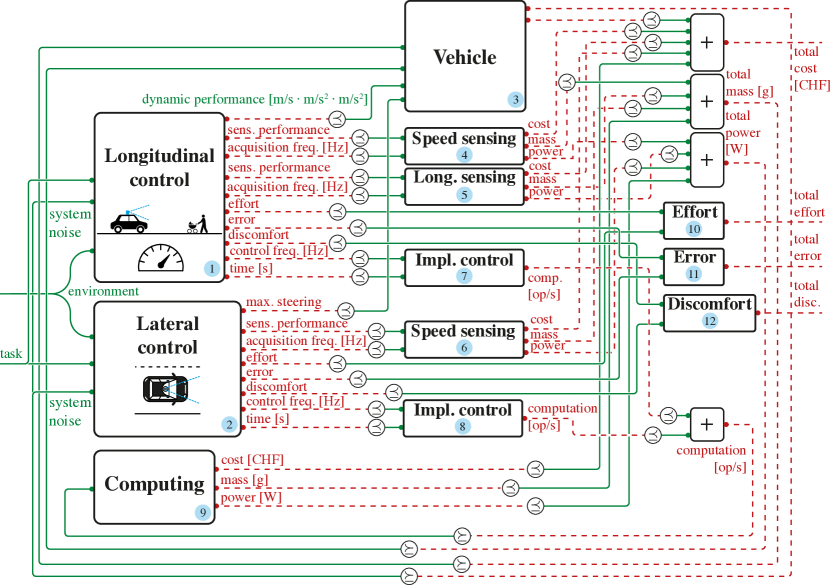
Figure 1: In this work we illustrate how to leverage a monotone theory of co-design to embed vehicle control design in a CDPI for a full robotic platform. The proposed results enable designers to formulate and solve the full task-driven co-design problem of a AV, characterized by choices related to hardware and software components. By fixing a task (e.g., desired speed and curvature of the trajectory considered), one can find the set of designs fulfilling the task and minimizing selected resources, including quality of execution, performance, effort (discomfort), costs, and safety.

Related literature

The need for design automation techniques has been recognized in [5, 6, 7, 8, 9], and traditionally researchers have been focusing on particular instances of co-design of sensing, actuation, and control [10, 11, 12, 13, 14, 15, 16, 17, 18, 19, 20, 21, 22, 23, 24, 25, 26, 27, 28].

The trade-offs characterizing sensing and control are predominant in the literature. Although sensor selection typically cannot be solved in a closed form, it has been shown that particular cases feature enough structure for efficient optimization schemes [10, 11]. In particular, the authors of [12] study sensing-constrained task-driven LQG control, and authors of [13, 14, 15, 16, 17] focus on the design of robots which can solve path planning problem. While in [18] researchers provide a framework to jointly optimize sensor selection and control, by minimizing the information a sensor needs to acquire, authors of [19, 20] propose techniques for optimal control with communication constraints. Methodologies to co-design robot architectures have been investigated in [21, 22, 23], and robot design trade-offs are presented in [24, 25, 26]. Finally [27] study optimal actuator placement in large-scale networks control, and [28] proposes techniques for algorithmic design for embodied intelligence in synthetic cells. In conclusion, while existing techniques for robotic platforms co-design highlight important trade-offs, they do not allow one to smoothly formulate and solve co-design problems involving control synthesis.

Statement of contributions

In this work we show how to leverage a monotone theory of co-design to frame the design of vehicle control strategies in the task-driven co-design of an entire AV. We show how to formulate each relevant control technique as a monotone design problem with implementation (MDPI), characterized by feasibility relations between tasks, control performance, accuracy, measurements’ and system’s noises, and intermittent observations schemes. Furthermore, we instantiate our discoveries in state-of-the-art case studies, in which we perform the task-driven co-design of an AV in urban driving scenarios, extending previous basic results presented in [3, 4] We illustrate how, given the model of the AV, a task, and behavior specifications, we can answer several questions regarding the optimal co-design of the full robotic platform.

II Monotone Co-Design Theory

(a) A MDPI is a monotone relation between posets of functionalities and resources.

(b) Series.

(c) Parallel.

(d) Loop.

Figure 2: MDPIs can be composed in different ways.

In this section, we summarize the main concepts related to the monotone theory of co-design [1, 2], which will be instrumental for the development of the key results in this work. The reader is assumed to be familiar with basic concepts of order theory [29] (some of which reported for convenience in Section -A). The monotone theory of co-design is based on the atomic notion of a MDPI.

Definition 1 (MDPI).

Given posets ${\color[rgb]{0.0,0.5,0.0}\mathcal{F}},{\color[rgb]{0.7,0.0,0.0}\mathcal{R}}$, (functionalities and resources), we define a MDPI as a tuple $\langle\mathcal{I}_{d},\mathsf{prov},\mathsf{reqs}\rangle$, where $\mathcal{I}_{d}$ is the set of implementations, and $\mathsf{prov}$, $\mathsf{reqs}$ are maps from $\mathcal{I}_{d}$ to ${\color[rgb]{0.0,0.5,0.0}\mathcal{F}}$ and ${\color[rgb]{0.7,0.0,0.0}\mathcal{R}}$, respectively:

$${\color[rgb]{0.0,0.5,0.0}\mathcal{F}}\xleftarrow{\mathsf{prov}}\mathcal{I}_{d}\xrightarrow{\mathsf{reqs}}{\color[rgb]{0.7,0.0,0.0}\mathcal{R}}.$$

We compactly denote the MDPI as $d\colon{\color[rgb]{0.0,0.5,0.0}\mathcal{F}}\leavevmode\hbox to18pt{\vbox to5.5pt{\text{[drawing]}}}{\color[rgb]{0.7,0.0,0.0}\mathcal{R}}$. Furthermore, to each MDPI we associate a monotone map $\bar{d}$, given by:

$$\begin{split}\bar{d}\colon{\color[rgb]{0.0,0.5,0.0}\mathcal{F}}^{\mathrm{op}}\times{\color[rgb]{0.7,0.0,0.0}\mathcal{R}}&\to\langle\mathcal{P}(\mathcal{I}_{d}),\subseteq\rangle\\ \langle{\color[rgb]{0.0,0.5,0.0}f}^{*},{\color[rgb]{0.7,0.0,0.0}r}\rangle&\mapsto\{i\in\mathcal{I}_{d}\colon(\mathsf{prov}(i)\succeq_{{\color[rgb]{0.0,0.5,0.0}\mathcal{F}}}{\color[rgb]{0.0,0.5,0.0}f})\wedge(\mathsf{reqs}(i)\preceq_{{\color[rgb]{0.7,0.0,0.0}\mathcal{R}}}{\color[rgb]{0.7,0.0,0.0}r})\},\end{split}$$

where $(\cdot)^{\mathrm{op}}$ reverses the order of a poset. The expression $\bar{d}({\color[rgb]{0.0,0.5,0.0}f}^{*},{\color[rgb]{0.7,0.0,0.0}r})$ returns the set of implementations (design choices) $S\subseteq\mathcal{I}_{d}$ for which functionalities ${\color[rgb]{0.0,0.5,0.0}f}$ are feasible with resources ${\color[rgb]{0.7,0.0,0.0}r}$. We represent a MDPI in diagrammatic form as in Fig. 2(a).

Remark (Monotonicity).

Consider a MDPI for which we know $\bar{d}({\color[rgb]{0.0,0.5,0.0}f}^{*},{\color[rgb]{0.7,0.0,0.0}r})=S$.

• ${\color[rgb]{0.0,0.5,0.0}f^{\prime}}\preceq_{{\color[rgb]{0.0,0.5,0.0}\mathcal{F}}}{\color[rgb]{0.0,0.5,0.0}f}\Rightarrow\bar{d}({\color[rgb]{0.0,0.5,0.0}f^{\prime}}^{*},{\color[rgb]{0.7,0.0,0.0}r})=S^{\prime}\supseteq S$. Intuitively, decreasing the desired functionalities will not increase the required resources;

• ${\color[rgb]{0.7,0.0,0.0}r^{\prime}}\succeq_{{\color[rgb]{0.7,0.0,0.0}\mathcal{R}}}{\color[rgb]{0.7,0.0,0.0}r}\Rightarrow\bar{d}({\color[rgb]{0.0,0.5,0.0}f}^{*},{\color[rgb]{0.7,0.0,0.0}r^{\prime}})=S^{\prime\prime}\supseteq S$. Intuitively, increasing the available resources cannot decrease the provided functionalities.

For related examples and detailed explanations we refer to our draft book [2].

Remark.

In practical cases, one can populate the feasibility relations of MDPIs with analytic relations (e.g. cost functions, precise relationships), numerical analysis of closed-form relations, and simulations (e.g., POMDPs). For detailed examples refer to [3, 4].

Definition 2.

Given a MDPI $d$, we define monotone maps

• $h_{d}\colon{\color[rgb]{0.0,0.5,0.0}\mathcal{F}}\to\mathsf{A}{\color[rgb]{0.7,0.0,0.0}\mathcal{R}}$, mapping a functionality to the minimum antichain of resources providing it;

• $h_{d}^{\prime}\colon{\color[rgb]{0.7,0.0,0.0}\mathcal{R}}{}\to\mathsf{A}{\color[rgb]{0.0,0.5,0.0}\mathcal{F}}$, mapping a resource to the maximum antichain of functionalities provided by it.

Solving MDPIs requires finding such maps, in the sense that one of the queries consists in fixing a desired functionality, and finding the set of minimum resources providing it. Furthermore, if such maps are Scott continuous, and posets involved are complete, one can rely on Kleene’s fixed point theorem to find the solution to the queries “fix a functionality and find minimum resources to achieve it” and “fix a resource and find maximum functionalities that can be achieved”. Individual MDPIs can be composed in several ways to form a co-design problem (a multigraph of co-design problems), allowing one to decompose a large problem into smaller subproblems, and to interconnect them. In Fig. 2 we report the main interconnections, and an exhaustive list is presented in [2]. Series composition happens when a functionality of a MDPI is required by another MDPI (e.g., the energy provided by a battery is needed by an electric motor to produce torque). The symbol “$\preceq$” is the posetal relation, which represents a co-design constraint: the resource one problem requires, cannot exceed the functionality another problem provides. Parallel composition formalizes decoupled processes happening together, and loop composition describes feedback. Notably, MDPIs are closed under compositions (i.e., a composition of MDPIs is an MDPI). We call the composition (multigraph) of MDPIs a co-design problem with implementation (CDPI).

III Functional decomposition approach

In this section, we report the key ingredients to understand our co-design approach, and to appreciate the results presented in Section IV [4, 3].

Figure 3: Classic data-flow diagram for an autonomous system.

First, it is important to distinguish between data-flow and logical dependencies. While Fig. 3 represents the classic data-flow diagram for an autonomous system, the co-design diagram in Fig. 1 formalizes logical dependencies through functional decomposition. In this kind of diagrams, the “arrows” are inverted: decision making needs state information, which is estimated through sensing data, provided by a sensor, which will have a cost, a weight, and some power consumption. The functional decomposition exercise results in a collection of sub-tasks, each of which can be abstracted as a MDPI (Fig. 4(a)). Embodied intelligence taks, and in particular control tasks, share a common interface, constituted of task-driven functionalities, such as performance (e.g., control effort and control error, comfort, safety), and functionalities shared with other parts of the system, such as scenarios/environments (e.g., robustness to system and measurement noises, density of obstacles). Providing functionalities comes at a price, which in robotics can be typically expressed in terms of monetary cost, power usage, computation effort, and mass of the system.

Starting from the task abstraction, one can turn the functional decomposition into a co-design diagram, by interconnecting dependent tasks and identifying common functionalities and resources (Fig. 4(b)).

(a) Co-design abstraction of tasks in embodied intelligence.

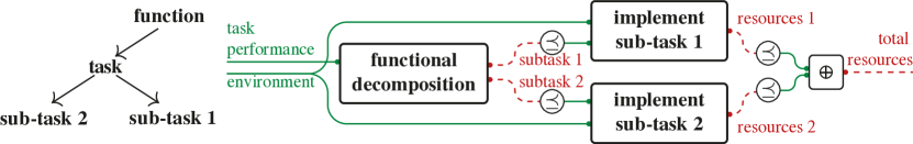
(b) Translating functional decomposition into co-design diagrams.

Figure 4: Functional decomposition provides us with sub-tasks, each of which we can model as a MDPI with environment and task performance as functionalities and cost, power, computation, power, and mass as resources. Interconnecting several tasks composing a functional decomposition is a MDPI (a task), and resources can be combined via an associative operation, such as $+$ or $\max$.

IV Co-design of vehicle control systems

Figure 5: General co-design problem for a control problem, highlighting the monotonicity in selected nuisances. For instance, if the probability of dropping observations increases, the tracking error will not decrease.

In [3] we show how to use the monotone theory of co-design presented in Section II to embed (variations of) LQG control design in an MDPI for an entire robotic platform. While finding interesting applications, the presented results were limited to a particular control technique. In the present work, we extend our theoretical results by showing how one can also embed the design of other important control schemes in a MDPI, in the context of designing a AV.

We present the considered control techniques, as well as their interpretation as MDPIs of the form as in Fig. 5. Theoretical results are sketched in Lemmas, intuitive proof sketches are provided in Section -B, and exhaustive proofs will be reported in an extended version of this work. The main idea is to show monotonicities between important quantities for control systems (as shown in Fig. 5), to embed their design in MDPIs and solve co-design problems for a robotic platform.

IV-A Vehicle model

Dynamics

We consider the kinematic single-track model from [30, 31] and extend it by considering model uncertainty. Consider $p_{r}=[x_{\mathrm{r}},y_{\mathrm{r}}]$ and  $p_{\mathrm{f}}=[x_{\mathrm{f}},y_{\mathrm{f}}]$ as the positions of the rear and front wheel with respect to the inertial coordinate frame. The heading $\theta$ describes the vehicle’s orientation (the angle between $p_{\mathrm{f}}-p_{r}$ and the inertial frame). The steering angle $\delta$ describes the front wheel orientation with respect to the vehicle’s one. Finally $l$ is the distance between front and rear axles. We can write the no-slip condition for the wheels with the following non-holonomic constraints:

$$-\dot{x}_{r}\sin(\theta)+\dot{y}_{r}\cos(\theta) =0,$$

$$-\dot{x}_{f}\sin(\theta+\delta)+\dot{y}_{f}\cos(\theta+\delta) =0.$$

We compute the rear velocity as $v_{\mathrm{r}}=\dot{p}_{r}(p_{\mathrm{f}}-p_{r})/\|p_{\mathrm{f}}-p_{r}\|$. By considering the state space $\bm{s}=[x_{\mathrm{r}},y_{\mathrm{r}},\theta,\delta,v_{\mathrm{r}}]$, and control inputs $\bm{u}=[v_{\mathrm{s}},a_{\mathrm{r}}]$, the dynamics read

$$\dot{\bm{s}}=f(\bm{s},\bm{u})+\bm{w}=\begin{bmatrix}v_{\mathrm{r}}\cos(\theta)\\ v_{\mathrm{r}}\sin(\theta)\\ v_{\mathrm{r}}\tan(\delta)/l\\ v_{\mathrm{s}}\\ a_{\mathrm{r}}\end{bmatrix}+\bm{w},$$ (1)

where $v_{\mathrm{s}}\in[\dot{\delta}_{\mathrm{min}},\dot{\delta}_{\mathrm{max}}]$ and $a_{\mathrm{r}}\in[\dot{v}_{\mathrm{r,min}},\dot{v}_{\mathrm{r,max}}]$ are control inputs, $\delta\in[\delta_{\mathrm{min}},\delta_{\mathrm{max}}]\subset[-\pi/2,\pi/2]$, $v_{\mathrm{r}}\in[v_{\mathrm{r,min}},v_{\mathrm{r,max}}]$, and $\bm{w}$ is a standard Brownian process with effective noise covariance $\mathbf{W}$. The motion of the front wheel is then:

$$\dot{x}_{\mathrm{f}} =v_{\mathrm{f}}\cos(\theta+\delta),$$

$$\dot{y}_{\mathrm{f}} =v_{\mathrm{f}}\sin(\theta+\delta),$$

$$v_{\mathrm{f}} =v_{\mathrm{r}}/\cos(\delta).$$

Furthermore, the angular velocity is $\omega=v_{\mathrm{f}}\sin(\delta)/l$.

Measurement model

We consider the discrete-time measurement model

$$\bm{y}_{k}=\gamma_{k}(\bm{s}_{k}+\bm{v}_{k}),$$ (2)

where $\gamma_{k}\in\{0,1\}$ represents an intermittent observations process (e.g., linear Gaussian Bernoulli, linear Gaussian Markov, and linear Gaussian semi-markov [32]), and $\bm{v}_{k}$ is a standard Brownian process with effective noise covariance $\mathbf{V}$ (parametrizing the fidelity of the measurement, i.e., the quality of the sensor).

Remark.

In this work we will use, among others, the Loewner order on the set of Hermitian matrices of order $n$, denoted $\mathcal{M}^{n}$. Take two Hermitian matrices $\mathbf{A},\mathbf{B}$. We say $\mathbf{A}\preceq_{\mathcal{L}}\mathbf{B}$ if and only if $\mathbf{B}-\mathbf{A}$ is positive semi-definite.

Definition 3.

Consider sequences of Hermitian matrices $\mathbf{P}$, $\mathbf{Q}$ of length $N\in\mathbb{N}$. We define the poset of sequences of Hermitian matrices of length $N$ by setting $\mathbf{P}\preceq_{\mathcal{S}}\mathbf{Q}$ if and only if $\mathbf{P}_{i}\preceq_{\mathcal{L}}\mathbf{Q}_{i}$ for all $i\in N$.

IV-B State estimation

Following the literature, we consider an extended Kalman filter (EKF) with the discrete-time measurement model in Eq. 2. We summarize the estimation procedure.
Initialization:

$$\hat{\bm{s}}(t_{0})=\mathbb{E}\left[\bm{s}(t_{0})\right],\ \mathbf{P}_{0|0}=\mathbb{E}[(\bm{s}(t_{0})-\hat{\bm{s}}(t_{0}))(\bm{s}(t_{0})-\hat{\bm{s}}(t_{0}))^{\intercal}].$$

Prediction update: Solve

$$\dot{\hat{\bm{s}}}(t) =f(\hat{\bm{s}}(t),\bm{u}(t)),$$

$$\dot{\mathbf{P}}(t) =\mathbf{F}(t)\mathbf{P}(t)+\mathbf{P}(t)\mathbf{F}(t)^{\intercal}+\mathbf{W}(t),\ \mathbf{F}(t)=\frac{\partial f}{\partial\bm{s}}\big{|}_{\hat{\bm{s}}(t),\bm{u}(t)},$$

with $\hat{\bm{s}}(t_{k-1})=\hat{\bm{s}}_{k-1|k-1}$, and $\mathbf{P}(t_{k-1})=\mathbf{P}_{k-1|k-1}$, to obtain $\hat{\bm{s}}_{k|k-1}=\hat{\bm{s}}(t_{k})$ and $\mathbf{P}_{k|k-1}=\mathbf{P}(t_{k})$.

Measurement update: Compute

$$\mathbf{K}_{k} =\mathbf{P}_{k|k-1}(\mathbf{P}_{k|k-1}+\mathbf{V})^{-1},$$

$$\hat{\bm{s}}_{k|k} =\hat{\bm{s}}_{k|k-1}+\mathbf{K}_{k}(\bm{y}_{k}-\hat{\bm{s}}_{k|k-1}),$$

$$\mathbf{P}_{k|k} =(\mathbf{I}-\mathbf{K}_{k})\mathbf{P}_{k|k-1},$$

where $\mathbf{P}$ represents the covariance estimate.

Given this model, one can prove the monotonicity of the covariance estimate with respect to the noise and measurement covariances, and to the probability of loosing observations. These results will be important when building the control MDPIs.

Lemma 1.

The sequence of covariance estimates $\mathbf{P}$ produced by the EKF is monotone in $\mathbf{V}$ and $\mathbf{W}$. In other words:

$$\langle\mathbf{V},\mathbf{W}\rangle\preceq_{\mathcal{L}\times\mathcal{L}}\langle\mathbf{V}^{\prime},\mathbf{W}^{\prime}\rangle\Rightarrow\mathbf{P}(\mathbf{V},\mathbf{W})\preceq_{\mathcal{S}}\mathbf{P}(\mathbf{V}^{\prime},\mathbf{W}^{\prime}).$$

Lemma 2.

The sequence of covariance estimates $\mathbf{P}$ is monotone in the probability of dropping observations.

IV-C Control

We instantiate the functional decomposition approach for the self-driving task of a AV. In particular, one can decompose this task into lateral and longitudinal control (Fig. 6(a)). Longitudinal control can be then split into speed tracking and emergency braking.

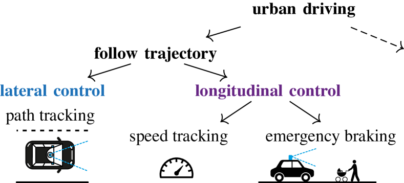
(a) Functional decomposition for urban driving.

(b) Stanley control.

(c) Pure pursuit control.

Figure 6: (a) Functional decomposition for the self-driving task of a AV. (b,c): Geometric lateral control with Stanley and pure pursuit techniques.

IV-C1 Lateral control

The lateral control action can be formulated as choosing the steering velocity to track a given reference path. The vehicle’s speed is typically considered constant at each time step (decoupling the longitudinal and lateral control problems). Controllers consider the first four states/equations of Eq. 1 (denoted by $\bm{z}$) and receive a state estimate at discrete times $\hat{\bm{z}}_{k}=\bm{z}_{k}+\bm{\mu}_{k}$, where $\bm{\mu}_{k}$ is a standard Brownian process with effective noise covariance $\mathbf{P}_{k}$ (as per state estimation procedure and measurement model). The control error $\bm{e}(t)=\begin{bmatrix}e_{p}(t)&\theta_{e}(t)\end{bmatrix}^{\intercal}$ is generally expressed as the distance between the vehicle’s front axle and the reference point on the path, and the angle between the vehicle’s heading and the tangent to the path at the reference point. In the following, we list the standard lateral control techniques we considered, and their properties [30, 33].

Stanley control

This is a geometric type of vehicle control based on the single-track bicycle model (i.e., the orientation and position of the front wheel with respect to the reference path are considered for generating control actions). Given the error, one can write the desired steering angle at any time as $\delta(t)=\theta_{e}(t)+\arctan(ge_{p}(t)/v_{\mathrm{f}})$, where $g$ is the Stanley gain (Fig. 6(b)). We denote by $e_{p,\mathrm{tot}}$ the total control positional error and by $\delta_{\mathrm{tot}}$ the total control effort along a path.

Lemma 3.

The total Stanley control lateral tracking error $e_{p,\mathrm{tot}}$ is monotonic in $\mathbf{W}$ and the sequence of estimate covariances $\mathbf{P}$.

Lemma 4.

The total Stanley control effort $\delta_{\mathrm{tot}}$ is monotonic in $\mathbf{W}$ and the sequence of estimate covariances $\mathbf{P}$.

Pure Pursuit

Given a reference path, the control law fits a semi-circle through the vehicle’s current configuration to a point on the reference path, which has a distance (called “lookahead”) $L$ from the car (Fig. 6(c)). We consider the algorithm presented in [34], and extend it by requiring the vehicle’s heading to be tangent to the circle. The curvature of the semi-circle is $\kappa=2\sin(\alpha)/L$. Given a constant rear velocity $v_{\mathrm{r}}$, the angular velocity of a vehicle following the semi-circle is $\dot{\theta}=2v_{\mathrm{r}}\sin(\alpha)/L$. From Eq. 1, one has $\delta=\arctan(2l\sin(\alpha)/L)$, where $\alpha$ is the angle between the vehicle’s orientation and the vector from the current configuration $\langle x,y\rangle$ and the target one $\langle x_{\mathrm{t}},y_{\mathrm{t}}\rangle$. Again, the control error $\bm{e}(t)=[e_{p}(t),\theta_{e}(t)]$ is expressed as the distance between the vehicle’s front axle and the reference point on the path, and the angle between the vehicle’s heading and the tangent to the path at the reference point. The control procedure is then: a) Find current location of the vehicle, b) find the path-point closest to the vehicle, c) find the goal point, d) transform it to the vehicle coordinates, e) calculate the curvature and set the steering angle accordingly, f) update vehicle’s position [33].

Lemma 5.

The total pure pursuit control lateral tracking error $e_{p,\mathrm{tot}}$ is monotonic in $\mathbf{W}$ and in the sequence of estimate covariances $\mathbf{P}$.

Lemma 6.

The total pure pursuit control effort $\delta_{\mathrm{tot}}$ is monotonic in $\mathbf{W}$ and in the sequence of estimate covariances $\mathbf{P}$.

LQR with adaptive state space control

The error is given by $\bm{e}(t)=[e_{p},\theta_{e}]$, where $e_{p}$ is the positional error perpendicular to the path tangent, and $\theta_{e}$ is the difference between the path tangent and the vehicle orientation. The method linearizes the error dynamics around $[0,0]$ at every time instant, and solves an infinite horizon optimization problem for the linearized system. The error dynamics for small errors can be formulated as

$$\dot{\bm{e}}(t)=\begin{bmatrix}0&v_{\mathrm{r}}\\ 0&0\end{bmatrix}\bm{e}(t)+\begin{bmatrix}0\\ v_{\mathrm{r}}/l\end{bmatrix}\delta(t),$$

and the quadratic cost function to minimize takes the form

$$J(T)=\int_{0}^{T}\bm{e}(t)^{\intercal}\mathbf{Q}\bm{e}(t)+\delta^{2}(t)\mathbf{R}\text{d}t.$$

Lemma 7.

The total LQR control lateral tracking error $e_{p,\mathrm{tot}}$ is monotonic in $\mathbf{W}$ and in the sequence of estimate covariances $\mathbf{P}$.

Lemma 8.

The total LQR control effort $\delta_{\mathrm{tot}}$ is monotonic in $\mathbf{W}$ and in the sequence of estimate covariances $\mathbf{P}$.

Nonlinear Model Predictive Control (NMPC)

The NMPC method with receding horizon strategy aims at minimizing the positional error $\bm{e}_{k}$ (expressed with respect to the point on the path which is closest to the vehicle’s center of mass at instant $k$) and control effort $\delta$ over $n_{\mathrm{h}}\in\mathbb{N}$ steps. The formulation of the optimization problem is as follows:

$$u_{k}^{\star} =\mathop{\mathrm{argmin}}_{U_{k}}\sum_{i=0}^{n_{\mathrm{h}}+1}e_{k+i}^{\intercal}\mathbf{Q}e_{k+i}+u_{k+i}^{\intercal}\mathbf{R}u_{k+i},$$

$$U_{k} =\{u_{k},\ldots,u_{k+n_{\mathrm{h}}-1}\},$$

$$e_{k} =\hat{e}(t_{k}),$$

$$e_{k+i} =\int_{k+i-1}^{k+i}v_{\mathrm{f}}\sin(\theta_{e}(\tau)-u(\tau))\text{d}\tau,$$

where $\dot{\theta}_{e}$ follows Eq. 3, and where one only applies $u_{0}^{\star}$ each time. This technique is characterized by different path approximation techniques (e.g., linear, quadratic, and cubic), integration techniques, and by different lateral error reference points on the vehicle (e.g., rear or center of gravity).

Lemma 9.

The total NMPC lateral control tracking error is monotonic in $\mathbf{W}$ and the sequence of estimate covariances $\mathbf{P}$.

Lemma 10.

The total NMPC lateral control effort is monotonic in $\mathbf{W}$ and the sequence of estimate covariances $\mathbf{P}$.

IV-C2 Speed control

The control goal is to track a certain target velocity $v_{\mathrm{t}}$. From Eq. 1, the velocity dynamics are $\dot{v}_{\mathrm{r}}=a_{\mathrm{r}}+\bm{w}_{v_{\mathrm{r}}}$. The system receives an estimation of the current velocity through the measurement model at each time instant $k$: $\hat{v}_{\mathrm{r},k}=v_{\mathrm{r},k}+\rho_{k}$, where $\rho_{k}$ is a standard Brownian process with effective noise covariance $q_{k}$ (as per state estimation procedure and measurement model). The control input is typically formulated via a PID control scheme (i.e., just by choosing specific tuning parameters $k_{\mathrm{p}},k_{\mathrm{i}},k_{\mathrm{d}}$):

$$u(t)=k_{\mathrm{p}}(v_{\mathrm{t}}-\hat{v}(t))+k_{\mathrm{i}}\int_{0}^{t}(v_{\mathrm{t}}-\hat{v}(\tau))\text{d}\tau-k_{\mathrm{d}}\frac{\partial\hat{v}}{\partial t}.$$

Lemma 11.

The total PID control tracking error is monotonic in $\mathbf{W}$ and the sequence of estimate covariances $q$.

Lemma 12.

The total PID control effort is monotonic in $\mathbf{W}$ and the sequence of estimate covariances $q$.

IV-C3 Brake control

The topic of (emergency) braking has been treated in detail in [4], where longitudinal sensors (ordered by their performance, expressed via false positives, false negatives, and accuracy curves) were used to detect potential obstacles. Clearly, the more uncertain the obstacle detection, the more potentially dangerous will the braking maneuver be. We delay the treatment of this particular topic to future works, and refer the interested reader to [4].

IV-D Control as MDPI

We can now combine the results presented for estimation (Section IV-B) and for control (Section IV-C) to formulate a co-design theorem.

Theorem 13.

The presented controllers (PID, Stanley, Pure Pursuit, LQR, and NMPC) can be written as MDPIs of the form in Fig. 5.

Proof.

The proof of the theorem follows easily from the proofs of the previous lemmas. ∎

Discussion

The presented theorem allows one to frame standard vehicle control systems as MDPIs. This result provides an interface to smoothly include control synthesis in the robot co-design problem. We remark that theory and results can be generalized to the case of uncertain parameters [35].

V Co-design of an autonomous vehicle

We now show the ability of the proposed framework to embed aspects of task-driven vehicle control synthesis into the co-design of an entire platform. The guiding example of this work is the one of a AV, but the same principle can be generalized to other autonomous systems and abstraction levels [36, 37]. We first present the setting of the case study, then detail the modeling of the AV as an interconnection of MDPIs, and finally describe selected results to showcase the potential of the approach.

V-A Setting

We consider urban scenarios, extending and customizing the ones proposed in the CommonRoads framework [38]. We implemented the mentioned autonomy pipelines in our own simulator. While the proposed approach has been tested on several scenarios (e.g., racing, pursue-evasion, exploration), for exposition purposes we focus on two examples. We first look at the case in which an AV needs to perform a $90\mathrm{°}$ degrees, and then look at a lane change example (Fig. 7(a), Fig. 7(b)). The task of the AV consists in following a trajectory (with customized curvature severity) at a desired speed. By fixing a particular task we want to find the autonomy pipeline for the AV to minimize selected resource usages.

V-B Co-design model

We now consider the co-design diagram for an AV presented in Fig. 1, and describe the principles behind each block. While we explicitly showed how to think about control schemes as MDPIs, this can be done for the other blocks as well, and all the conditions can be checked empirically or analytically. The co-design diagram can be thematically subdivided into control, perception, implementation, and evaluation blocks.

V-B1 Control

Hereafter, we describe the longitudinal and lateral design blocks. Both provide the fulfillment of a task, in a specific environment (e.g., characterized by the time of the day, or the density of obstacles on the road [4]), and with robustness to a particular uncertainty in the AV model. The vehicle is characterized by a dynamic performance (e.g., parametrized by the reachable speed, acceleration, and steering angle) . For the control laws to be implemented, observations (with particular uncertainties) from sensors are required (for the longitudinal case, to estimate speed and presence of obstacles, and for the lateral case, to estimate position and heading), which are received at particular frequencies. Control techniques will need to be implemented at certain frequencies and will cause specific control efforts and errors (in the longitudinal control case, expressed in terms of velocity deviation, and in the lateral control case, as lateral deviation), as well as discomfort (e.g., intensity of the steering, or gravity of accelerations) and dangerous situations (e.g., increasing the probability to hit obstacles). For these blocks, models can be obtained analytically and via simulations.

V-B2 Perception

Observations are provided to controllers via sensors at particular frequencies, requiring monetary costs, power consumptions, and mass to be transported ( , , ). For these blocks, models are typically obtained from sensor catalogues, photogrammetry, and simulations. Particular observation schemes can also be artificially perturbed, and observation dropping schemes can be applied. For details see [4].

V-B3 Implementation

Control routines need to be implemented ( , ) at certain frequencies requiring computation, provided by physical computers . Computers come at a monetary cost, power consumption, and mass to be transported. The computation required for particular processes can be estimated via benchmarking (indeed, different implementations of the same concept will require different computational performance). Models for computers can be derived from catalogues.

V-B4 Evaluation

Different choices for the above thematic blocks will give rise to different outcomes, each characterized by various performance metrics, such as total monetary cost of the platform, control effort, control error, danger, and discomfort ( , , ). Furthermore, the mass and power required by the components will be provided by the phyiscal vehicle. Here, models can be customized to fit specific applications.

V-C Co-design results

Variable	Options
PP	$L\in\{0.01,0.05,0.5,1.0,2.0\}$
Stanley	$g\in\{0.05,0.1,0.5,1.0,1.5,2.0\}$
LQR	$\mathbf{R}\in\{0.001,0.05,0.5,1.0,10.0\}$, $\mathbf{Q}\in\{0.1\cdot\mathbb{1},1.0\cdot\mathbb{1},10.0\cdot\mathbb{1},0.2\cdot(\mathbb{1}-0.9e_{3}),1.0\cdot(\mathbb{1}-0.9e_{3}),5.0\cdot(\mathbb{1}-0.9e_{3})\}$
NMPC	$n_{\mathrm{h}}\in\{10.0,15.0,20.0,25.0\}$, $\mathbf{R}\in\{0.05,0.5,1.0,5.0\}$, $\mathbf{Q}\in\{0.01\cdot\mathbb{1},0.1\cdot\mathbb{1},1.0\cdot\mathbb{1},10.0\cdot\mathbb{1}\}$
PID	$k_{\mathrm{p}}\in\{0.1,0.5,1.0,2.0\}$, $k_{\mathrm{I}}\in\{0.01,0.1,0.5,1.0\}$, $k_{\mathrm{d}}\in\{0.01,0.05,0.1,1,0\}$
Computers	RPi 4B, Jetson Nano/TX1,2/AGX Xavier, Xavier NX
Sensors	Basler Ace251gm/222gm/13gm/7gm/5gm/15um, Flir Pointgrey, KistlerSMotion, OS032/128, OS232/128, HDL 32/64

TABLE I: Variables and options for the AV co-design problem.

We now solve the co-design problem presented in the previous section focusing on a selection of queries. By fixing a task (i.e., a desired scenario, speed, and average curvature), we can characterize optimal design solutions in terms of monetary cost, control effort, control error, danger, and discomfort. The design space is characterized by the controllers presented in Section IV and their parameters, various sensors for the different perception blocks, and computer models, all listed for convenience in Table I. For simplicity of exposition, we do not consider obstacle detection modeling (already treated in depth in [4]), and focus on path tracking and speed control. Note that this represents just a sample of the designs we can look at. (For instance, we neglect control frequencies).

(a) Trade-off (antichain) of total control error and effort for a $90\mathrm{°}$ turn, with low curvature at 8 m/s, with corresponding design choices.

(b) Trade-off (antichain) of cost and control error for lane change with high curvature at 15 m/s, with corresponding design choices.

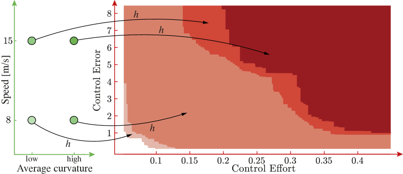
(c) Monotonicity of the MDPI: higher cruise speed or curvature will require higher control error and effort.

Figure 7: Trade-offs for selected case studies. The red lines represent antichains, and the red areas the corresponding upper sets of resources.

V-C1 Control effort and control error trade-offs

We first consider a case in which we want the vehicle to perform a $90\mathrm{°}$ turn with a low curvature, at 8 m/s, with a standard battery electric vehicle. By solving the co-design problem, we obtain a Pareto front of optimal designs, which we can interpret by looking at its 2D-projections. We first look at the trade-offs between total control effort and total control error (Fig. 7(a)). In red, the Pareto front of optimal solutions, which are not comparable since no instance leads simultaneously to lower control error and control effort. The upper set of feasible resources is given in solid red. Furthermore, for each point lying on the Pareto front, we are able to report details about the optimal designs, including the chosen control technique and its parameters, as well as considered sensors and computer. As one can see in Fig. 7(a), low control effort (discomfort) can be achieved with a specific combination of controllers and parameters, at the cost of an important control error. Similarly, low control error can be achieved by another design, with increased control effort.

V-C2 Monetary cost and control error trade-offs

We look at the task of lane changing, choosing a high curvature and a speed of 15 m/s. We can now solve the co-design problem with the updated task. To showcase the richness of the insights we can produce, we now report the trade-offs between monetary costs and control error for the AV (Fig. 7(b)). Clearly, to achieve lower control error one needs to pay more. Interestingly, investing 39,000 CHF instead of 54,000 CHF only deteriorates the error by 10%.

V-C3 Monotonicity

We consider the task of lane changing, now showcasing the monotonicity properties of the developed framework. We look at varying tasks, starting from a low speed of 8 m/s and low curvature and increasing speed to 15 m/s and high curvature. Fig. 7(c) shows multiple co-design queries. In particular, for each functionality (left plot), we report the Pareto front and the upper set of optimal resources (right plot), by using the map defined in Definition 2. Monotonicity can be seen in the dominance of subsequent Pareto fronts (right plot), illustrated in increasing red tonality via inclusion of the upper sets.

VI Conclusions

We presented how a monotone theory of co-design allows one to simultaneously synthesize state-of-the-art vehicle control systems and design the entire robotic platform. The proposed approach promotes modularity and compositionality, and captures heterogeneous task-driven design abstraction levels, ranging from control synthesis and parameter tuning to hardware selection.

Outlook

The proposed results open the stage for important further developments. First, we want to connect the present work with our efforts in modeling sensor curves [4], to consider scenarios with moving obstacles and include more granular sensor modeling approaches. Second, we want to enlarge the library of control schemes which one can embed in the co-design framework (e.g., studying sliding-mode controllers, dynamic switching of controllers), better model digitalisation, include the notion of planning in the models, and present extensive case studies. Third, we want to leverage our recent results in the co-design theory to query for robustness against multiple, heterogeneous tasks (indeed, one can argue that urban driving will require the ability to solve different ones). Fourth, we want to study systems which might show complications when embedded in our framework (e.g., Hammerstein-Wiener systems). Finally, we want to showcase compositionality by connecting the present work to our work in mobility [37].

-A Background on orders

Definition 4 (Poset).

A poset is a tuple $\mathcal{P}=\langle P,\preceq_{\mathcal{P}}\rangle$, where $P$ is a set and $\preceq_{\mathcal{P}}$ is a partial order, defined as a reflexive, transitive, and antisymmetric relation.

Definition 5 (Opposite of a poset).

The opposite of a poset $\langle P,\preceq_{\mathcal{P}}\rangle$ is the poset $\langle P,\preceq_{\mathcal{P}}^{\mathrm{op}}\rangle$, which has the same elements as $\mathcal{P}$, and the reverse ordering.

Definition 6 (Product poset).

Let $\langle P,\preceq_{\mathcal{P}}\rangle$ and $\langle Q,\preceq_{\mathcal{Q}}\rangle$ be posets. Then, $\langle P\times Q,\preceq_{\mathcal{P}\times\mathcal{Q}}\rangle$ is a poset with

$$\langle p_{1},q_{1}\rangle\preceq_{\mathcal{P}\times\mathcal{Q}}\langle p_{2},q_{2}\rangle\Leftrightarrow(p_{1}\preceq_{\mathcal{P}}p_{2})\wedge(q_{1}\preceq_{\mathcal{Q}}q_{2}).$$

This is called the product poset of $\langle P,\preceq_{\mathcal{P}}\rangle$ and $\langle Q,\preceq_{\mathcal{Q}}\rangle$.

Definition 7 (Monotonicity).

A map $f\colon\mathcal{P}\to\mathcal{Q}$ between two posets $\langle P,\preceq_{\mathcal{P}}\rangle$, $\langle Q,\preceq_{\mathcal{Q}}\rangle$ is monotone iff $x\preceq_{\mathcal{P}}y$ implies $f(x)\preceq_{\mathcal{Q}}f(y)$. Monotonicity is compositional.

-B Proof sketches

Proof sketch for Lemma 1.

One can prove the statement by induction. The monotonicity holds in the initialization. To prove the induction step, one can first write the prediction update, and leverage properties of the differential Lyapunov equation involved. Finally, one uses the results of the induction step in the measurement update, to prove the result. ∎

Proof sketch for Lemma 2.

The statement can be proven by following the substitution principle [3]. If the estimator is given a set of observations, it can simulate having less (i.e., having a higher dropping probability) by artificially ignoring selected samples. This can also be proven analytically, by comparing measurement updates in the EKF in the two cases. ∎

Proof sketch for Lemma 3.

First, one can derive the error dynamics

$$\dot{e}_{p}(t) =v_{\mathrm{f}}\sin(\theta_{e}(t)-\delta(t))+\rho_{e}(t),$$ (3)

$$\dot{\theta}_{e}(t) =-v_{\mathrm{f}}\sin(\delta(t))/L+\bm{w}_{\theta},$$

where $\rho_{e}$ and $\bm{w}_{\theta}$ are Brownian processes as per given models. By leveraging properties of the system and measurement noises, one can then show that at any time instant, by larger $\mathbf{W}$ or $\mathbf{P}$, one cannot obtain a smaller expected total lateral error (to parity of initial condition). ∎

Proof sketch for Lemma 4.

The expected lateral positional and orientation errors converging more rapidly to zero imply a commanded steering angle converging more rapidly to zero in expectation. This can be formally proven by taking the expectation of the steering angle formulation as presented in the Stanley part. ∎

Proof sketch for Lemma 5.

First, one can derive the lateral error dynamics

$$\dot{e}_{p}=-v_{\mathrm{r}}e_{\mathrm{along}}(t)\sin(\delta(t))/L+\rho_{e}(t),$$

where $\rho_{e}$ is a Brownian process and

$$e_{\mathrm{along}}(t)=\begin{bmatrix}x_{\mathrm{t}}-x(t)&y_{\mathrm{t}}-y(t)\end{bmatrix}\cdot\begin{bmatrix}\cos(\theta(t))\\ \sin(\theta(t))\end{bmatrix}.$$

Then, one can leverage properties of the system and measurement noises to prove the statement. ∎

Proof sketch for Lemma 6.

This can be shown by following the procedure in Lemma 5 and looking at the behavior of $\delta(t)$. ∎

Proof sketch for Lemma 7 and Lemma 8.

One can derive the expected error dynamics for the original, nonlinear system, and leveraging properties of the noise perturbations, one can derive both monotonicity results. ∎

Proof sketch for Lemma 11.

One can easily write the expression for the expected value of the speed tracking error between any two control steps. Given the properties of the perturbations in the system model and in the measurement model, one can show that this expression is monotonic in system noise and state estimation uncertainty. ∎

Proof sketch for Lemma 12.

By explicitly looking at the expression for the expected value of the acceleration resulting from the control, one proceed as for Lemma 11 and show the monotonicity. ∎

Proof sketch for Lemma 9 and Lemma 10.

First, one can derive the error dynamics, which are equivalent to Eq. 3. One can prove that at each step, the map describing the dependency of the optimal (initial) control input on the initial lateral error is s-shaped (for positive definite $\mathbf{Q}$). Furthermore, in the presence of heading error, the s-shaped curve is translated proportionally along the input axis. From these facts, one can prove the statements. ∎

References

- [1] A. Censi, “A mathematical theory of co-design,” arXiv preprint arXiv:1512.08055, 2015.
- [2] A. Censi, J. Lorand, and G. Zardini, Applied Compositional Thinking for Engineers, 2022, work in progress book. [Online]. Available: https://bit.ly/3qQNrdR
- [3] G. Zardini, A. Censi, and E. Frazzoli, “Co-design of autonomous systems: From hardware selection to control synthesis,” in 2021 European Control Conference (ECC), 2021, pp. 682–689.
- [4] G. Zardini, D. Milojevic, A. Censi, and E. Frazzoli, “Co-design of embodied intelligence: A structured approach,” in 2021 IEEE/RSJ International Conference on Intelligent Robots and Systems (IROS), 2021, pp. 7536–7543.
- [5] Q. Zhu and A. Sangiovanni-Vincentelli, “Codesign methodologies and tools for cyber–physical systems,” Proceedings of the IEEE, vol. 106, no. 9, pp. 1484–1500, 2018.
- [6] B. Zheng, P. Deng, R. Anguluri, Q. Zhu, and F. Pasqualetti, “Cross-layer codesign for secure cyber-physical systems,” IEEE Transactions on Computer-Aided Design of Integrated Circuits and Systems, vol. 35, no. 5, pp. 699–711, 2016.
- [7] A. Saoud, P. Jagtap, M. Zamani, and A. Girard, “Compositional abstraction-based synthesis for interconnected systems: An approximate composition approach,” IEEE Transactions on Control of Network Systems, vol. 8, no. 2, pp. 702–712, 2021.
- [8] S. A. Seshia, S. Hu, W. Li, and Q. Zhu, “Design automation of cyber-physical systems: Challenges, advances, and opportunities,” IEEE Transactions on Computer-Aided Design of Integrated Circuits and Systems, vol. 36, no. 9, pp. 1421–1434, 2016.
- [9] A. Prorok, M. Malencia, L. Carlone, G. S. Sukhatme, B. M. Sadler, and V. Kumar, “Beyond robustness: A taxonomy of approaches towards resilient multi-robot systems,” arXiv preprint arXiv:2109.12343, 2021.
- [10] S. Joshi and S. Boyd, “Sensor selection via convex optimization,” IEEE Transactions on Signal Processing, vol. 57, no. 2, pp. 451–462, 2008.
- [11] V. Gupta, T. H. Chung, B. Hassibi, and R. M. Murray, “On a stochastic sensor selection algorithm with applications in sensor scheduling and sensor coverage,” Automatica, vol. 42, no. 2, pp. 251–260, 2006.
- [12] V. Tzoumas, L. Carlone, G. J. Pappas, and A. Jadbabaie, “Lqg control and sensing co-design,” IEEE Transactions on Automatic Control, 2020.
- [13] Y. Zhang and D. A. Shell, “Abstractions for computing all robotic sensors that suffice to solve a planning problem,” in 2020 IEEE International Conference on Robotics and Automation (ICRA). IEEE, 2020, pp. 8469–8475.
- [14] D. A. Shell, J. M. O’Kane, and F. Z. Saberifar, “On the design of minimal robots that can solve planning problems,” IEEE Transactions on Automation Science and Engineering, pp. 1–12, 2021.
- [15] S. Smith, A. Saoud, and M. Arcak, “Monotonicity-based symbolic control for safety in real driving scenarios,” 2021.
- [16] S. Karaman and E. Frazzoli, “High-speed motion with limited sensing range in a poisson forest,” in 2012 IEEE 51st IEEE Conference on Decision and Control (CDC). IEEE, 2012, pp. 3735–3740.
- [17] Y. V. Pant, H. Yin, M. Arcak, and S. A. Seshia, “Co-design of control and planning for multi-rotor uavs with signal temporal logic specifications,” in 2021 American Control Conference (ACC). IEEE, 2021, pp. 4209–4216.
- [18] T. Tanaka and H. Sandberg, “Sdp-based joint sensor and controller design for information-regularized optimal lqg control,” in 2015 54th IEEE Conference on Decision and Control (CDC). IEEE, 2015, pp. 4486–4491.
- [19] S. Tatikonda and S. Mitter, “Control under communication constraints,” IEEE Transactions on automatic control, vol. 49, no. 7, pp. 1056–1068, 2004.
- [20] D. Soudbakhsh, L. T. Phan, O. Sokolsky, I. Lee, and A. Annaswamy, “Co-design of control and platform with dropped signals,” in Proceedings of the ACM/IEEE 4th international conference on cyber-physical systems, 2013, pp. 129–140.
- [21] A. A. C. Collin, “A systems architecture framework towards hardware selection for autonomous navigation,” Ph.D. dissertation, Massachusetts Institute of Technology, 2019.
- [22] A. Collin, A. Siddiqi, Y. Imanishi, E. Rebentisch, T. Tanimichi, and O. L. de Weck, “Autonomous driving systems hardware and software architecture exploration: optimizing latency and cost under safety constraints,” Systems Engineering, vol. 23, no. 3, pp. 327–337, 2020.
- [23] G. Bravo-Palacios, A. Del Prete, and P. M. Wensing, “One robot for many tasks: Versatile co-design through stochastic programming,” IEEE Robotics and Automation Letters, vol. 5, no. 2, pp. 1680–1687, 2020.
- [24] M. Lahijanian, M. Svorenova, A. A. Morye, B. Yeomans, D. Rao, I. Posner, P. Newman, H. Kress-Gazit, and M. Kwiatkowska, “Resource-performance tradeoff analysis for mobile robots,” IEEE Robotics and Automation Letters, vol. 3, no. 3, pp. 1840–1847, 2018.
- [25] J. M. O’Kane and S. M. LaValle, “Comparing the power of robots,” The International Journal of Robotics Research, vol. 27, no. 1, pp. 5–23, 2008.
- [26] J.-P. Merlet, “Optimal design of robots,” in Robotics: Science and systems, 2005.
- [27] B. Guo, O. Karaca, T. Summers, and M. Kamgarpour, “Actuator placement under structural controllability using forward and reverse greedy algorithms,” IEEE Transactions on Automatic Control, vol. 66, no. 12, pp. 5845–5860, 2020.
- [28] A. Pervan and T. D. Murphey, “Algorithmic design for embodied intelligence in synthetic cells,” IEEE Transactions on Automation Science and Engineering, vol. 18, no. 3, pp. 864–875, 2020.
- [29] B. A. Davey and H. A. Priestley, Introduction to lattices and order. Cambridge university press, 2002.
- [30] B. Paden, M. Čáp, S. Z. Yong, D. Yershov, and E. Frazzoli, “A survey of motion planning and control techniques for self-driving urban vehicles,” IEEE Transactions on intelligent vehicles, vol. 1, no. 1, pp. 33–55, 2016.
- [31] J. Kong, M. Pfeiffer, G. Schildbach, and F. Borrelli, “Kinematic and dynamic vehicle models for autonomous driving control design,” in 2015 IEEE intelligent vehicles symposium (IV). IEEE, 2015, pp. 1094–1099.
- [32] A. Censi, “Kalman filtering with intermittent observations: Convergence for semi-markov chains and an intrinsic performance measure,” IEEE Transactions on Automatic Control, vol. 56, no. 2, pp. 376–381, 2010.
- [33] M. Rokonuzzaman, N. Mohajer, S. Nahavandi, and S. Mohamed, “Review and performance evaluation of path tracking controllers of autonomous vehicles,” IET Intelligent Transport Systems, vol. 15, no. 5, pp. 646–670, 2021.
- [34] R. C. Coulter, “Implementation of the pure pursuit path tracking algorithm,” Carnegie-Mellon UNIV Pittsburgh PA Robotics INST, Tech. Rep., 1992.
- [35] A. Censi, “Uncertainty in monotone codesign problems,” IEEE Robotics and Automation Letters, vol. 2, no. 3, pp. 1556–1563, 2017.
- [36] G. Zardini, N. Lanzetti, M. Pavone, and E. Frazzoli, “Analysis and control of autonomous mobility-on-demand systems,” Annual Review of Control, Robotics, and Autonomous Systems, vol. 5, no. 1, 2022.
- [37] G. Zardini, N. Lanzetti, A. Censi, E. Frazzoli, and M. Pavone, “Co-design to enable user-friendly tools to assess the impact of future mobility solutions,” arXiv preprint arXiv:2008.08975, 2022.
- [38] M. Althoff, M. Koschi, and S. Manzinger, “Commonroad: Composable benchmarks for motion planning on roads,” in 2017 IEEE Intelligent Vehicles Symposium (IV). IEEE, 2017, pp. 719–726.