A Shared Parameter Model for Systolic Blood Pressure Accounting for Data Missing Not at Random in the HUNT Study.

Abstract

In this work, blood pressure eleven years ahead is modeled using data from a longitudinal population-based health survey, the Trøndelag Health (HUNT) Study, while accounting for missing data due to dropout between consecutive surveys ($20-50\%$). We propose and validate a shared parameter model (SPM) in the Bayesian framework with age, sex, body mass index, and initial blood pressure as explanatory variables. Further, we propose a novel evaluation scheme to assess data missing not at random (MNAR) by comparing the predictive performance of the fitted SPM with and without conditioning on the missing process. The results demonstrate that the SPM is suitable for inference for a dataset of this size (cohort of $64385$ participants) and structure. The SPM indicates data MNAR and gives different parameter estimates than a naive model assuming data missing at random. The SPM and naive models are compared based on predictive performance in a validation dataset. The naive model performs slightly better than the SPM for the present participants. This is in accordance with results from a simulation study based on the SPM where we find that the naive model performs better for the present participants, while the SPM performs better for the dropouts.

Keywords: longitudinal studies, missing data, INLA (integrated nested Laplace approximations), dropout, health survey

1 Introduction

This work aims to establish and validate a predictive model for future systolic blood pressure using data from a longitudinal population-based health survey, the Trøndelag Health (HUNT) Study, while accounting for missing data due to dropout.

Elevated blood pressure increases the risk of developing diseases related to the brain, heart, blood vessels, and kidney (Lewington et al., 2002; Tozawa et al., 2003; Rapsomaniki et al., 2014). It affects more than 1.1 billion people worldwide and accounts for over 10.8 million deaths per year, thereby surpassing smoking as the leading preventable cause of death for middle-aged and older adults (Zhou et al., 2017; Murray et al., 2020). Early detection, prevention, and treatment of elevated blood pressure are of high priority in public health strategies (World Health Organizatoin, 2013). Thus, obtaining unbiased, accurate models for predicting future blood pressure is of great interest in medical research (Whelton, 1994). Longitudinal population-based health survey provide valuable datasets for constructing such models but are rarely without missing data. For instance, each HUNT survey include 50000 to 80000 participants, but $20-50\%$ of the participants are lost to follow-up in consecutive surveys (Krokstad et al., 2013; Åsvold et al., 2021). Proper handling of missing data is vital to obtain unbiased inference (Gad and Darwish, 2013; Little and Rubin, 2019, Chap. 1.3, 6), and how to handle missing data depends on the missing process.

Based on available literature (Anderson Jr et al., 1994; Whelton, 1994; Brown et al., 2000; Jiang et al., 2016; Espeland, 2020), we suggest a predictive model of future blood pressure with age, sex, body mass index (BMI), and initial blood pressure as explanatory variables. All participants used in this study have full records for the explanatory variables. Missing data can be categorized and described in terms of three missing processes; missing completely at random (MCAR), missing at random (MAR), and missing not at random (MNAR) (Little and Rubin, 2019, Chap. 1.3, 6). If the probability of dropout, i.e. of missing future blood pressure values, is independent of all observed and unobserved data, including the missing response variables and all explanatory variables, the data is MCAR. It is reasonable that the probability of dropping out depends on age, and hence MCAR is disregarded for this work. The data is MAR if the probability of missingness depends on the observed data, but is independent of the unobserved data. Missing processes that are MCAR or MAR are ignorable, meaning unbiased inference can be performed without modeling the missing process. Data that is neither MCAR nor MAR is MNAR (Gad and Darwish, 2013; Little and Rubin, 2019, Chap. 6). If the part of the future blood pressure which can not be explained by age, sex, BMI, and initial blood pressure, affects the probability of dropping out, the data is MNAR. This can be thought of as (unknown) explanatory variables not included in the models. It is reasonable to assume that there are health related variables that influence both blood pressure and the probability of drop out. Thus, we argue that in a predictive model for future blood pressure we should consider that data might be MNAR. If data is MNAR the missing process must be modeled simultaneously with the original model to obtain unbiased inference (Little and Rubin, 2019, Chap. 1.3, 6).

Even though the assumption of data MAR is often not fulfilled, many of the available software packages and methods described in the literature assume data to be MAR (Balakrishnan, 2009; Rhoads, 2012; Little and Rubin, 2019; Mohan and Pearl, 2021; Griswold et al., 2021). However, several studies, especially in biostatistics, have accounted for missing data under the assumption of data MNAR. (Wu and Carroll, 1988; Little, 1993; Diggle and Kenward, 1994; Follmann and Wu, 1995; Little, 1995; Albert and Follmann, 2000; Molenberghs et al., 2008; Howe et al., 2016). Popular choices for models accounting for data MNAR include the pattern mixture model, selection model, and shared parameter model (SPM) (Heckman, 1979; Wu and Carroll, 1988; Little, 1993; Henderson et al., 2000; Linero and Daniels, 2018; Little and Rubin, 2019; Griswold et al., 2021,  Chap. 15.4). The SPM is based on the idea of a commonly shared variable affecting both the measurement process and the missing process. Given this variable, the two marginal densities are conditionally independent. It has been used to model longitudinal data subject to MNAR in several studies (Wu and Carroll, 1988; Follmann and Wu, 1995; Thomas et al., 1998; Pulkstenis et al., 1998; Vonesh et al., 2006; Creemers et al., 2010). In this work, we propose a Bayesian SPM for future blood pressure. The model fits the framework of Bayesian latent Gaussian model and is suitable for Bayesian inference using computationally efficient Integrated Nested Laplace Approximations (INLA) (Rue et al., 2009, 2017; Martino and Riebler, 2019; Gómez-Rubio, 2020; Steinsland et al., 2014).

Molenberghs et al. stated that ”each MNAR model fit to a set of observed data can be reproduced exactly by a MAR counterpart” (Molenberghs et al., 2008, p. 371). Hence, the choice between models eventually comes down to choosing the most likely model assumptions (Enders, 2011). Recent research has proven that taking the approach of causal modeling and formulating the models through missingness graphs can give theoretical understanding and asymptotic performance guarantees (Mohan and Pearl, 2021). To the best of our knowledge, the literature provides little insight into practical validation of model performance on data MNAR. The current standard seems to be the use of simulation studies to check the reproducibility of the model. i.e., how well the original parameters are reproduced on simulated data, and sensitivity analysis to check the robustness of the models (Enders, 2011; Steinsland et al., 2014; Kaciroti and Little, 2021).

In this work, we validate the models on a validation dataset. First, predictive performance of the SPM and a naive model assuming the data to be MAR are compared based on the proper scoring rules (Gneiting and Raftery, 2007) continuous ranked probability score (CRPS) and Brier score. Second, we propose a new method to evaluate if data is MNAR based on the SPM. The main idea is that if data is MNAR, the missing status has information about the quantity of interest. Therefore, we compare the predictive performance of the SPM with and without conditioning on missing status.

The main contributions of this paper is the SPM for future blood pressure based on data from the HUNT Study, the demonstration of the SPM’s applicability for a large case study and new insight from the proposed validation schemes.

Section 2 provides background about latent Gaussian models and missing data theory. Section 3 introduces the blood pressure case study including the HUNT Study, the proposed models, and methods for inference and validation. The results from the case study are presented in Section 4. Section 5 consists of several simulation sensitivity studies based on the HUNT Study. Section 6 summarizes and discusses our findings.

2 Background Theory

This section briefly introduces latent Gaussian models and commonly used models and methods for missing data.

2.1 Latent Gaussian Models

Latent Gaussian models (LGMs) fall within a subclass of the structured additive regression models (Rue et al., 2009) meaning the response $y_{i}$ belongs to the class of exponential families. Hence, the mean $E(y_{i})=\mu$ is linked to a structured additive predictor $\eta$ through a link function $h(\mu)$ such that $h(\mu)=\eta$. For the structured additive regression models $\eta$ is defined as follows (Fahrmeir et al., 2007),

$$h(\mu)=\eta=\alpha+\sum_{k=1}^{n_{\beta}}\beta_{k}z_{k}+\sum_{j=1}^{n_{f}}f^{(j)}(u_{j})+\epsilon.$$

Here $\{\beta_{k}\}$ represents the linear effects of explanatory variables $\boldsymbol{z}$, $\{f^{(j)}(.)\}$ represents unknown functions of explanatory variables $\boldsymbol{u}$, and $\epsilon$ is an unstructured term. All LGMs have Gaussian prior distributions of $\alpha$, $\{\beta_{k}\}$, $\{f^{(j)}(.)\}$ and $\epsilon$. All models used in this work belong to the class of LGMs.

2.2 Missing Data

In this section we follow Little and Rubin (2019) and let $\boldsymbol{y_{i}}$ be the set of $j$ measurements on the $i$th subject. Then $\boldsymbol{y_{i}}$ can be divided into an observed part $\boldsymbol{{y_{i}}_{o}}$ and a missing part $\boldsymbol{{y_{i}}_{m}}$, $\boldsymbol{y_{i}}=(\boldsymbol{{y_{i}}_{o}},\boldsymbol{{y_{i}}_{m}})$. Let $\boldsymbol{m_{i}}$ be the vector of,

$$m_{ij}=\begin{cases}1&\text{if ${y_{ij}}$ is missing}\\ 0&\text{otherwise}.\end{cases}$$

Then the full conditional of $\boldsymbol{y_{i}}$ and $\boldsymbol{m_{i}}$ is given as follows,

$$g(\boldsymbol{{y_{i}}_{o}},\boldsymbol{{y_{i}}_{m}},\boldsymbol{m_{i}}|\boldsymbol{\theta},\boldsymbol{\psi})$$ (1)

where the parameters $\boldsymbol{\theta}$ and $\boldsymbol{\psi}$ describes the measurement process and missing process, respectively (Gad and Darwish, 2013; Little and Rubin, 2019, Chap. 6.2). The data is MCAR if the missing process $g(\boldsymbol{m_{i}}|\boldsymbol{{y_{i}}_{o}},\boldsymbol{{y_{i}}_{m}},\boldsymbol{\psi})=g(\boldsymbol{m_{i}}|\boldsymbol{\psi})$. The data is MAR if $g(\boldsymbol{m}|\boldsymbol{{y_{i}}_{o}},\boldsymbol{{y_{i}}_{m}},\boldsymbol{\psi})=g(\boldsymbol{m_{i}}|\boldsymbol{{y_{i}}_{o}},\boldsymbol{\psi})$. If the data is neither MCAR nor MAR, the data is, by definition, MNAR. If data is MNAR, the missing process must be modeled simultaneously with the measurement process to obtain unbiased inference (Little and Rubin, 2019, Chap. 6.2), and several models have been proposed including pattern mixture models and selection models (Little and Rubin, 2019). In this work, a class of selection models known as shared parameter models (SPMs) is used. From now on, let $\boldsymbol{x_{i}}$ be the set of fully observed explanatory variables and $\epsilon_{i}$ be an unobserved within-subject random effect with hyperparameter $\gamma$. (Little and Rubin, 2019, Chap. 15.2) defined SPM as follows:

$$g(\boldsymbol{y_{i}},\boldsymbol{m_{i}},\epsilon_{i}|\boldsymbol{x_{i}},\boldsymbol{\theta},\boldsymbol{\psi},\gamma)=g(\boldsymbol{y_{i}}|\boldsymbol{x_{i}},\epsilon,\boldsymbol{\theta})g(\boldsymbol{m_{i}}|\boldsymbol{x_{i}},\epsilon_{i},\boldsymbol{\psi})g(\epsilon_{i}|\boldsymbol{x_{i}},\gamma).$$ (2)

This model assumes that both the measurement and dropout processes depend on a shared latent variable $\epsilon_{i}$. MAR is then a special case with $g(m_{i}|\boldsymbol{x_{i}},\epsilon_{i},\boldsymbol{\psi})=g(m_{i}|\boldsymbol{x_{i}},\boldsymbol{\psi})$ (Vonesh et al., 2006).

3 Case Study: A Blood Pressure Predictive Model Based on the HUNT Study.

3.1 The HUNT Study and Explanatory Analyses

The HUNT Study is a longitudinal population-based health survey in central Norway and the study protocols have been described in detail previously by (Krokstad et al., 2013; Åsvold et al., 2021) (Supplementary material A). Every adult citizen in the now former county of Nord-Trøndelag were invited to participate in clinical examinations and questionnaires in 1984-86 (HUNT1), 1995-97 (HUNT2), 2006-08 (HUNT3), and 2017-19 (HUNT4) (Krokstad et al., 2013; Åsvold et al., 2021). In this study, observations of systolic blood pressure ($BP$), age ($age$), body mass index ($BMI$) and sex ($sex$, 0 for females and 1 for males) are used. Following Tobin et al. (2005) $BP$ is adjusted by adding 15 mmHg for all participants who self-reported using BP medication. When needed a subscript indicates the HUNT survey of the observation (e.g. $BP_{2}$ denotes BP observed at HUNT2). We define a training dataset (HUNT2 cohort) with observations of initial blood pressure ($BP_{I}=BP_{2}$), $age$, $BMI$ and $sex$ from HUNT2, together with future blood pressure ($BP_{F}=BP_{3}$) from HUNT3 and a missing indicator $m$ (1 if $BP_{F}$ is missing in HUNT3, 0 if present). Of $60385$ participants in HUNT2 without missing data on explanatory variables, $43.1\%$ of the cohort were missing in HUNT3.

Summary statistics and units for the observations in the HUNT2 cohort are given in Table 1, together with observations grouped on missing status. In all analyses, $BP_{F}$, $BP_{I}$, $age$ and $BMI$ observations are standardized by the corresponding sample mean and standard deviation in the HUNT2 cohort.

Table 1: The sample mean and standard deviation of $BP_{F}$, $BP_{I}$, $age$, and $BMI$ and proportion of female/male participants in the HUNT2 cohort are displayed in the third column. The fourth and fifth columns display sample mean for the present and missing participants in addition to proportions of present/missing participants for the whole cohort and per sex.

Summary of the HUNT2 cohort
Variable	Unit	HUNT2	Present in HUNT3	Missing in HUNT3
$BP_{3}$ ($BP_{F})$	mmHg	-	136.1	-
$BP_{2}$ ($BP_{I}$)	mmHg	139.5 (23.6)	135.2	145.0
$age_{2}$	years	50.0 (17.1)	47.0	54.01
$BMI_{2}$	kg/$m^{2}$	26.4 ( 4.1)	26.2	26.6
$sex$			56.9 %	43.1 %
female	0	53.0 %	59.3 %	40.7 %
male	1	47.0 %	54.3 %	45.7 %

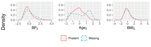
Figure 1: Smoothed empirical density of $BP_{I}$ ($BP_{2}$), $age$, and $BMI$ for all participants in the HUNT2 cohort.

In Figure 1 and Table 1 we find clear differences between the present and missing participants for $age$ and $BP_{I}$ ($BP_{2}$). Middle-aged participants are less likely to drop out than young or elderly participants, and those with higher blood pressure are more likely to be missing. This suggests that the data is at least MAR.

We defined a validation dataset (HUNT3 cohort) consisting of participants with observations of blood pressure ($BP_{I}=BP_{3}$), $age$, $BMI$ and $sex$ in HUNT3, and future blood pressure ($BP_{F}=BP_{4}$) and missing status in HUNT4. Of $50201$ participants in HUNT3, $33.3\%$ of the cohort dropped out before HUNT4. See Table 5 in Supplementary material B for a summary of the HUNT3 cohort.

3.2 A Shared Parameter Model for Blood Pressure

We set up a shared parameter model (SPM) for $BP_{F}$ and the missing process using $age$, $sex$, $BMI$, and $BP_{I}$, as explanatory variables in the framework of a LGM as presented in Section 2.1. Let ${BP_{F}}_{i}$ and $m_{i}$ represent future blood pressure and missing status for individual $i$. The likelihoods are chosen to be Gaussian with identity link for $BP_{F}$ and Bernoulli with logit link for $m_{i}$; $BP_{F_{i}}\sim N(\eta_{BP_{i}},\sigma_{BP}^{2})$ and $m_{i}\sim Bernoulli(p_{i})$ with $logit(p_{i})=\eta_{m_{i}}$. From the general formula of LGMs in Section 2.1 the explanatory variables can be included either as linear effects or as non-linear effects. Based on the work by Espeland (2020) and the analyses in Supplementary material C we chose to include $age$ in the missing process as a non-linear effects, and all other explanatory variables as well as age in the blood pressure model as linear effects. Further we introduce a shared parameter $\epsilon_{i}$ in both linear predictors, and an association parameter $c$ for the missingness model;

$$\eta_{BPi}=\alpha_{0}+\alpha_{BP}{BP_{I}}_{i}+\alpha_{age}age_{i}+\alpha_{BMI}{BMI}_{i}+\alpha_{sex}sex_{i}+\epsilon_{i}$$ (3)

$$\eta_{mi}=\beta_{0}+\beta_{BP}{BP_{I}}_{i}+f(age_{i})+\beta_{BMI}{BMI}_{i}+\beta_{sex}sex_{i}+c{\epsilon}_{i},$$

where the shared parameters $\epsilon_{i}$ are assumed to be independent Gaussian $\epsilon_{i}\sim N(0,\sigma_{\epsilon}^{2})$ and $f()$ is a random walk of order two with variance $\sigma_{age}$, as defined in Supplementary material C. To avoid identifiability issues between the shared parameter $\epsilon$ and the likelihood of $BF_{F}$ we fix $\sigma_{BP}^{2}$ to a small value ($\sigma_{BP}^{2}=0.001^{2}$). All regression parameters $\alpha_{0}$, $\alpha_{BP}$, $\alpha_{age}$, $\alpha_{BMI}$, $\alpha_{sex}$, $\beta_{0}$, $\beta_{BP}$, $\beta_{BMI}$, and $\beta_{sex}$ are given independent priors $N(0,{10^{3}}^{2})$, and $\sigma_{age}^{2}$ and $\sigma_{\epsilon}^{2}$ are assigned independent gamma priors, $\text{Gamma}(1,5\cdot 10^{5})$. We expect the shared parameter to influence the missing process similarly or less than the standardized explanatory variables. Therefore, the association parameter $c$ is given an informative prior $c\sim N(0,1^{2})$. A sensitivity study is conducted for this prior, see Supplementary material E.

When the association parameter $c=0$, the models for $BP_{F}$ and $m$ are independent and we have a model that assumes data MAR. We refer to this model as the naive model, and it is used as a benchmark model.

For simplicity we introduce some notation. Let $\boldsymbol{x_{i}}=({BP_{I}}_{i},age_{i},BMI_{i},sex_{i})$ be the explanatory variables and $\boldsymbol{y_{i}}=({BP_{F}}_{i},m_{i})$ the response variables for individual $i$. Further let $X=(x_{i},..,x_{n})^{T}$ be the explanatory variables for all $n$ participants and $Y=(y_{1},...,y_{n})^{T}$ be the corresponding response variables in a cohort. When needed, we use a superscript to indicate the HUNT2 or HUNT3 cohort, i.e., $X^{2}$ are the explanatory variables from the HUNT2 cohort. Denote the modeling parameters by $\boldsymbol{\theta}$ = ($\alpha_{0}$, $\alpha_{BP}$, $\alpha_{age}$, $\alpha_{BMI}$, $\alpha_{sex}$, $\beta_{0}$, $\beta_{BP}$, $\beta_{BMI}$, $\beta_{sex}$, $\epsilon$, $f$, $c$, $\sigma_{\epsilon}$, $\sigma_{age}$) where $f$ refer to the Gaussian variables of the additive effect for $age$.

3.3 Inference

Conditioned on data $(X,Y)$ we can achieve posterior distributions for the parameters, $\pi(\boldsymbol{\theta}|X,Y)$. In this work, we are either interested in the marginal posterior of selected parameters $(j)$, $\pi(\theta^{(j)}|X,Y)$, or in the posterior predictive distribution for a new person with explanatory variables $\boldsymbol{x_{new}}$. This posterior predictive distribution is given by

$$\pi(\boldsymbol{y_{new}}|\boldsymbol{x_{new}},X,Y) =\int\pi(\boldsymbol{y_{new}},\boldsymbol{\theta}|\boldsymbol{x_{new}},X,Y)d\boldsymbol{\theta}$$

$$=\int\pi(\boldsymbol{y_{new}}|\boldsymbol{x_{new}},\boldsymbol{\theta})\pi(\boldsymbol{\theta}|X,Y)d\boldsymbol{\theta}.$$

The SPM suggested in Section 3.2 is a LGM, as described in Section 2.1 that meets the requirements for using the computationally efficient integrated nested Laplace approximations (INLA), see Steinsland et al. (2014) for more details for an analogous SPM. The latent Gaussian field consists of ($\alpha_{0}$, $\alpha_{BP}$, $\alpha_{age}$, $\alpha_{BMI}$, $\alpha_{sex}$, $\beta_{0}$, $\beta_{BP}$, $\beta_{BMI}$, $\beta_{sex}$, $\epsilon$, $f$, $c$) and the non-Gaussian hyperparameters are ($\sigma_{\epsilon}$, $\sigma_{age}$).

3.4 Validation Scheme Using the HUNT3 Cohort

We evaluate the prediction models obtained from the HUNT2 cohort using the HUNT3 cohort. For each participant $i$ in the HUNT3 cohort we get the predictive distributions $\boldsymbol{\hat{y}_{i}}\sim\pi(\boldsymbol{y_{i}^{3}}|\boldsymbol{x_{i}^{3}},X^{2},Y^{2})$ and specifically for the future blood pressure and missing status $\hat{BP_{Fi}}\sim\pi(BP_{Fi}^{3}|\boldsymbol{x_{i}^{3}},X^{2},Y^{2})$ and $\hat{m_{i}}\sim\pi(m_{i}^{3}|\boldsymbol{x_{i}^{3}},X^{2},Y^{2})$.

To evaluate the predictive performance we calculate the mean continuous rank probability score (CRPS) of $\hat{BP_{Fi}}$ and mean Brier score of $\hat{m_{i}}$ over all participants in the HUNT3 cohort. Let $F_{\hat{BP_{Fi}}}(x)$ be the cumulative probability distribution of $\hat{BP_{Fi}}$ and $BP_{Fi}$ the observed blood pressure in HUNT4 for participant $i$, then $CRPS(F,y)=\int_{-\infty}^{\infty}[F(x)-H(x-BP_{Fi})]^{2}dx$ where $H(u)$ is the Heaviside function (0 for $u<0$ and 1 for $u>0$). The blood pressure model can only be validated on the participants observed in both surveys. In contrast, the missing model can be evaluated for all participants.

Predictions from the SPM and the naive model are compared by their posterior mean for the HUNT3 cohort participants as well as their CRPS and Brier scores.

3.5 Evaluation of Missing not at Random by Conditioning on Missing Status

We introduce a novel method for validating if data is MNAR based on a SPM fitted to a training dataset (the HUNT2 cohort) and the difference in predictive performance for a validation dataset (the HUNT3 cohort) for predictors with and without conditioning on the missing status in the training dataset. For readability, we introduce the method using the notation of HUNT2 cohort and HUNT3 cohort, but the method is general.

If data are MNAR and the SPM is true, there is information about the shared parameter in the missing status, and conditioning on the missing status, i.e. the value of $m_{new}$ should give a better predictor. For each participant $i$ in the HUNT3 cohort we can, from the predictive distribution, $\pi(\boldsymbol{y_{i}^{3}}|\boldsymbol{x_{i}^{3}},X^{2},Y^{2})$ derive both the marginal predictive distribution for the future blood pressure $\hat{BP_{Fi}}\sim\pi(BP_{Fi}^{3}|\boldsymbol{x_{i}^{3}},X^{2},Y^{2})$ and the predictive distribution for the future blood pressure conditioned on the missing status $\hat{BP_{Fi}}|m_{i}\sim\pi(BP_{Fi}|\boldsymbol{x_{i}^{3}},X^{2},Y^{2},m_{i}^{3})$.

In practice, we can for a validation dataset only evaluate the predictions for the present participants, and not the dropouts, and we therefore compare the predictive performance of $\hat{BP}_{F_{new}}$ and $\hat{BP}_{F_{new}}|m_{new}=0$ for all presents participants. In this work, we have calculated the absolute error of the posterior mean predictions for each participant, and compare mean absolute errors (MAE) for the prediction with and without conditioning on missing status.

3.6 Software and Code

In this work, we use the R-INLA software (R-INLA, 2021). The R-INLA software supports fitting models with multiple likelihoods (Steinsland et al., 2014; Espeland, 2020; Gómez-Rubio, 2020, Chap. 6.4) which is the case for the SPM 3. All the code is available at the GitHub repository GitHub (2021). Since data can not be shared, to protect participants privacy, a completely simulated dataset is provided at GitHub (2021).

4 Results for the Blood Pressure Case Study

The shared parameter models (SPM) and the naive model introduced in Section 3 are fitted using the HUNT2 cohort as described in Section 3.2. This chapter presents and compares the posterior distributions of interest. Further, the predictive models are evaluated through predictive performance of the HUNT3 cohort, as described in Section 3.4 and Section 3.5.

4.1 Results for the HUNT2 Cohort

The posterior distributions of the estimates obtained by the SPM and the naive model , introduced in Section 3.2 and fitted to the HUNT2 cohort, can be seen in Figure 2. The posterior mean and $95\%$ credible intervals are presented in Table 6 in Supplementary material D.

For the blood pressure submodel in the SPM, we see that the effect of $BP_{I}$ ($\alpha_{BP}$) is the largest followed by $age$, $BMI$ and $sex$. The effect of $BMI$ and $sex$ are close to zero. The parameter estimates of the naive blood pressure model are of the same order as the SPM. However, all variables but age have weaker effects on future blood pressure in the naive model than the SPM. The difference is especially pronounced for $\alpha_{0}$ and $\alpha_{BP}$, suggesting the two models could result in different predictions.

For the missing process in the SPM, we see that $sex$ has the largest effect on the probability of dropping out, followed by $BP_{I}$ and $BMI$. The age effect is largest for the elderly and smallest for middle-aged participants (Figure 3). The SPM and the naive model are more similar in parameter estimates for the missing process than the blood pressure process. However, the parameter estimates of the naive model are shifted towards lower values than the SPM.

The association parameter $c$, connecting the two submodels 3 in the SPM is clearly positive, which implies an increase in the probability of dropping out for larger random effect. Hence, according to the SPM, participants with higher $BP_{F}$ than expected from the explanatory variables also have a larger probability of dropping out than expected from the explanatory variables.

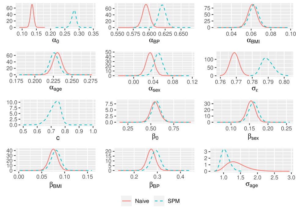
Figure 2: Posterior distribution of the latent field and hyperparameters for the SPM and naive model fitted to the HUNT2 cohort.

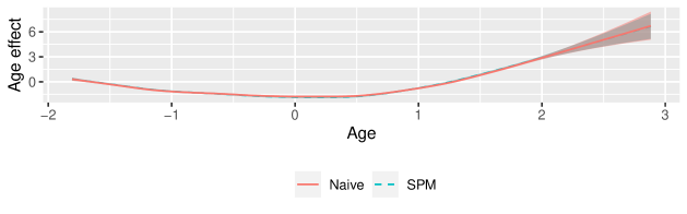
Figure 3: Age effect for the SPM and naive model fitted to the HUNT2 cohort with $95\%$ credible bands.

4.2 Results for Toy Example Participants

Since the data used in this work contains personal information, we consider three constructive toy example participants to explore the model presented in Section 3.2 and Section 3.4 on an individual level. We used a young and underweight female with low $BP_{I}$ (id1), a middle-aged and overweight female with average $BP_{I}$ (id2), and an old and obese female with severely high $BP_{I}$ (id3), see Table 2. For these participants, the effect of the association parameter on the probability of dropping out is plotted in Figure 4 for random effects between $-1.5$ and $1.5$ which corresponds to approximately two standard deviations of the random effect. We find that a larger value of the random effect gives a large probability of dropping out for all three toy example participants.

Table 2: Values of $BP_{I}$, $age$ and $BMI$ for three female toy example participants.

id	$BP_{I}^{*}$	$age^{*}$	$BMI^{*}$	$sex$	${BP_{I}}_{true}$	$age_{true}$	$BMI_{true}$
1	-2	-1.5	-2	female	92.2	24.4	18.2
2	0	0	0	female	139.5	50.0	26.4
3	2	1.5	2	female	186.7	75.7	34.6
* Standardized values

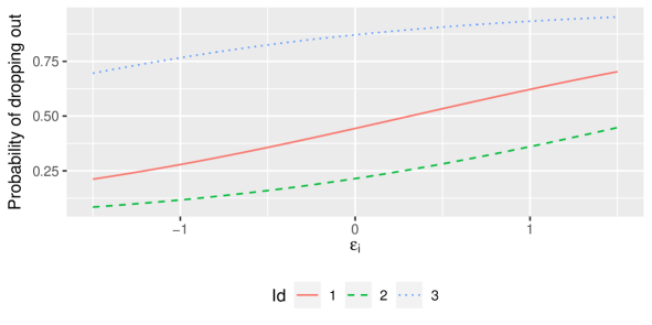
Figure 4: The probability of dropping out as a function of the individual random effect of the blood pressure model for three toy example participants specified in Table 2.

The posterior predictive distributions of $BP_{F}$ for the three simulated participants are plotted in Figure 5 for both the SPM and the naive model. For all toy example participants, the posterior predictive distribution from the SPM is shifted towards larger values than the naive model, and more so for id 1 and 3 who have more extreme explanatory variables.

Figure 5: Posterior predictive distribution of the future blood pressure ($BP_{F}$) for three toy example participants in Table 2 for the naive model and the SPM models. Vertical lines indicate posterior means.

4.3 Validation of Model Predictions for the HUNT3 Cohort

Table 3: CRPS score for predictions of systolic blood pressure in HUNT4 for the present participants. Brier score for mean predictions of the probability of drop out in HUNT4. All predictions are based on the HUNT3 cohort. The best score is indicated in bold.

	CRPS	Brier
		All	Present	Missing
SPM	0.4406	0.2082	0.1656	0.2937
Naive	0.4337	0.2072	0.1602	0.3014

For all HUNT3 participants, the predictive distributions are calculated as described in Section 3.3 using a model trained on the HUNT2 cohort. The empirical distributions of posterior mean predictions for participants in HUNT3 cohort are found in Figure 6(a), and for the $BP_{F}$ and in Figure 6(b) for probability of drop out $p$. For reference the empirical distribution for observed $BP_{F}$ is included for present participants in Figure 6(a). We see that on the SPM predicts slightly larger values for the $BP_{F}$ than the naive model on the population level. The distributions of mean predictions of the probability of dropping out are very similar. The SPM predicts a slightly higher average probability of dropping out than the naive model. We note that the differences between naive and SPM have little practical implication on population level, but for some individuals there can be differences of some practical significance.

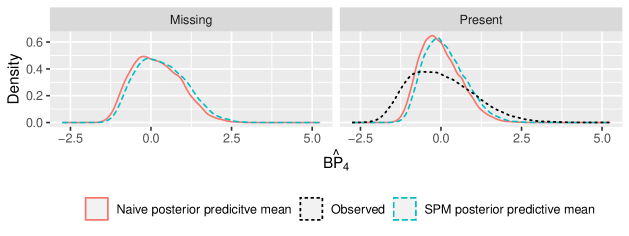
(a) Density over all participants in HUNT3 of the posterior mean of predicted future blood pressure $\hat{BP_{F}}_{i}$.

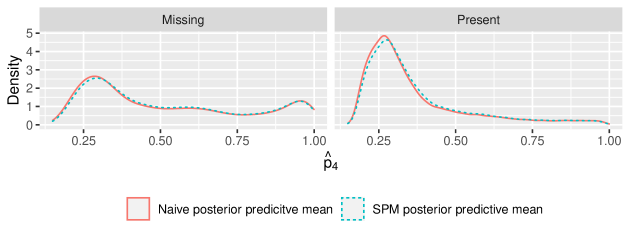
(b) Density over all participants in HUNT3 of the posterior mean of predicted probability of dropping out $\hat{p}_{i}$.

Figure 6: All plots display the participants grouped by missing status in the HUNT3 cohort.

We further evaluate the predictive performance for the HUNT3 cohort for the SPM and the naive model from the HUNT2 cohort as described in Section 3.4. Mean CRPS for $BP_{F}$ and mean Brier scores for the probability of drop out are given in Table 3. The mean CRPS is very similar for the SPM and naive model, but the CRPS for the naive model predictions is slightly smaller and hence the naive model performs slightly better. This might be explained by the fact that the missing participants do not affect the likelihood of the naive model. Hence, the model is optimized to perform well for the present participants. We explore this further in a simulation study in Section 5.2.

The Brier scores in Table 3 are slightly better for the naive model than for the SPM when evaluating for all participants. However, when grouped by missing status, the naive model performs better on the present participants, and the SPM performs better on the dropouts.

4.4 Evaluate of the Missing Not at Random Assumption

We evaluate the MNAR assumption by comparing the predictive performance of the SPM with and without conditioning on the missing status for the HUNT3 cohort as described in Section 3.5. The results are given in Table 4. We see that the mean absolute errors (MAEs) are very similar, but that the predictions for $\boldsymbol{BP_{4}}$ given $\boldsymbol{m_{4}}$ yield a slightly smaller error than not knowing $\boldsymbol{m_{4}}$. This suggests that some information from the missing process affects the $\boldsymbol{BP_{F}}$. A simulation study is conducted in Section 5.2, and a difference of $-0.0014$ is within what is to be expected when the SPM is true for similar training and validation datasets.

Table 4: Mean absolute error for $\boldsymbol{\hat{BP}_{F}}|m$ and $\boldsymbol{\hat{BP_{F}}}$. The best score is indicated in bold.

	$\boldsymbol{\hat{BP}_{F}}|m$	$\boldsymbol{\hat{BP_{F}}}$	MAE($\boldsymbol{\hat{BP}_{F}}|m$) - MAE($\boldsymbol{\hat{BP_{F}}}$)
MAE	0.6140	0.6155	-0.0014

5 Simulation Studies

We set up several simulation studies to explore the properties of the SPM, the naive model and the method validating MNAR by conditioning on missing status for datasets with the size and structure of the HUNT2 and HUNT3 cohort. In all simulation studies data sets for training models are simulated using the same number of participants and explanatory variables as in the HUNT2 cohort, i.e. $X=X^{2}$. Further, when simulating data, the parameters $\boldsymbol{\theta}=\boldsymbol{\theta^{true}}$ are set to the posterior mean estimates of the SPM and naive model fitted on the HUNT2 cohort, see Table 6, in Supplementary material D, in all simulation studies. When predictions are studied, simulated validation datasets are based on the same size and explanatory variables as the HUNT3 cohort, i.e. $X=X^{3}$ is used.

5.1 Simulation Study exploring Bias and Coverage

The aim of this simulation study is to study the properties of the posterior estimates for the SPM and the naive model in a situation similar to the HUNT2 cohort. 100 independent new response data (i.e. both future blood pressure $\boldsymbol{BP_{F}}$ and the missing status $\boldsymbol{m}$) are simulated using the SPM with parameters $\boldsymbol{\theta^{true}}$ and with explanatory variables as in the HUNT2 cohort, resulting in $Y^{(l)}$ for $l=1\dots 100$. For each of the data sets $(X^{2},Y^{(l)})$ both the SPM and the naive model are fitted. This gives posterior distributions $\pi(\boldsymbol{\theta}|X^{2},Y^{(l)})$. Each of these are summarized by the posterior mean and the coverage indicator of the true value in $95\%$ credibility interval.

The resulting mean posterior mean, bias, and coverage are found in Table 8 in Supplementary material F.

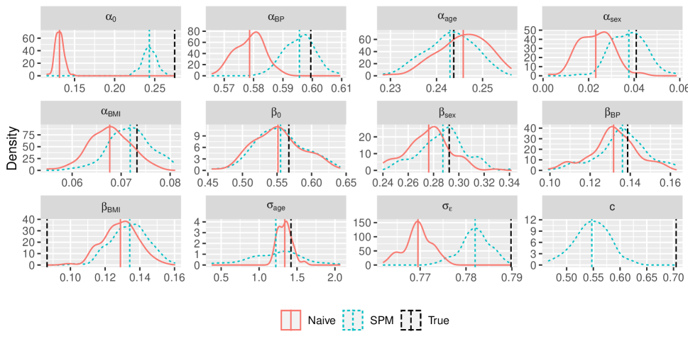
Figure 7: Distribution of posterior mean estimates on simulated data MNAR following the SPM as described in Section 5.1. The mean of posterior means for both the SPM and naive model and the true value are indicated by the vertical lines.

The distribution of the posterior means from the simulation study when the true parameters are the posterior mean estimates of the SPM can be seen in Figure 7. From Figure 7 we find that both the naive model and SPM are biased when the data is generated from the SPM. However, the SPM is less biased especially for the blood pressure model parameters (i.e. $\alpha_{0},\alpha_{PB},\alpha_{age},\alpha_{sex}$, and $\alpha_{BMI}$). The association parameter c has especially low coverage, see Table 8 in Supplementary material F).

We have also preformed a similar simulation study, but with data MAR by setting the association parameter $c=0$ when simulating data. The results are presented in Supplementary material F When the data is MAR, both the SPM and naive model have very little bias, and in particular the association parameter $c$ is centered around zero and has good coverage.

5.2 Simulation Study for Predictions

The aim of this simulation study is to learn about the predictive performance. Following the procedure in Section 5.1 a data sets mimicking the HUNT2 cohort, $(X^{2},Y)$, and $l=1\dots 100$ data sets mimicking the HUNT3 cohort, $(X^{3},Y^{(l)})$, are simulated using the SPM with parameters $\boldsymbol{\theta^{true}}$. Corresponding posterior distributions based on the simulated HUNT2 cohort $\pi_{SPM}(\boldsymbol{\theta}|X^{2},Y)$ and $\pi_{naive}(\theta|X^{2},Y)$ are found based on the SPM and the naive model, respectively. From these, posterior predictive distributions are achieved, and the predictive performance is evaluated for each participant in the simulated data set $(X^{3},Y^{(j)})$ as described in Section 3.4 by the CRPS and Brier score. A large advantage for the simulated data sets is that predictive performance can be evaluated not only for present participants, but also for those that are missing, and we include them.

Further we compare the predictive performance conditioned on missing status
$\pi_{SPM}(Y^{(l)}|\boldsymbol{m}^{l},X^{3},\boldsymbol{\theta})$ with $\pi_{SPM}(Y^{(l)}|X^{3},\boldsymbol{\theta})$ through MAE as described in Section 3.5.

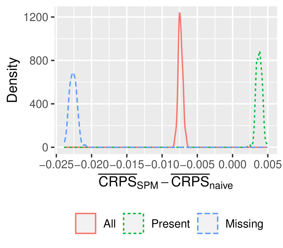
(a) Difference in mean CRPS score for the SPM and naive model with 100 simulations

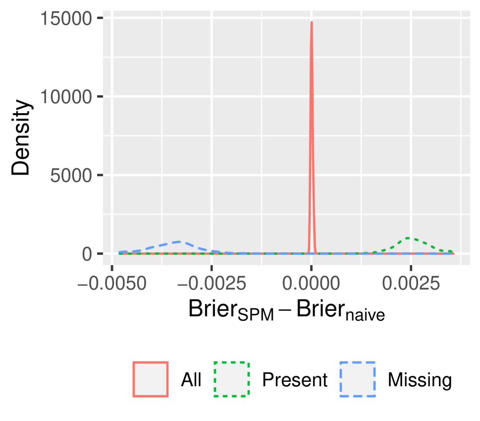
(b) Difference in mean Brier score for the SPM and naive model with 100 simulations

Figure 8: Plots for differences in mean scores for participants grouped by missing status in the HUNT3 cohort.

Figure 8(a) displays the distribution of the difference between the mean CRPS for the SPM and the naive model. This difference is displayed for all simulated participants (present/missing) and grouped on missing status. We see that the SPM performs better for all participants and the dropouts, but the naive model performs better on present participants. This demonstrates that for our case study even if the data is MNAR and follows the SPM, the naive model is expected to obtain a better CRPS than the SPM when only evaluating for present participants (and the missing participants can not be used for evaluation!).

Figure 8(b) shows the distribution of the difference in Brier score for all, missing and present participants. We see similar results here, the SPM predicts best for missing participants and the naive model predicts best for the present participants.

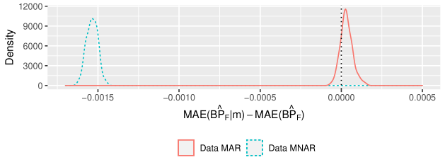
Figure 9: Difference in mean absolute error (MAE) of the predictions of $\boldsymbol{\hat{BP_{F}}|m}$ and $\boldsymbol{\hat{BP_{F}}}$ when the data is MNAR and MAR. The vertical line indicates zero.

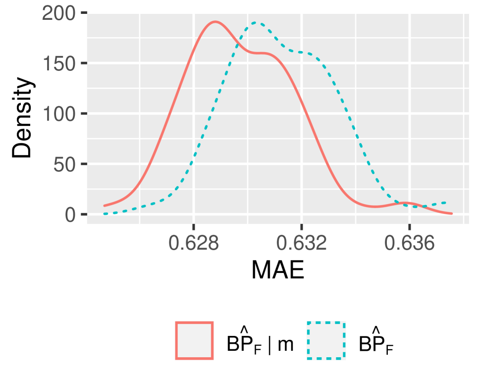
(a) Data MNAR

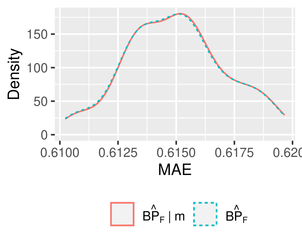
(b) Data MAR

Figure 10: Distribution of the mean absolute error MAE of the posterior mean prediction for future blood pressure obtained from the validation scheme presented in Section 5.2

For data MNAR, we can see from Figure 10(a) that the distribution of MAEs for the 100 simulations is shifted towards lower values when the missing status is known when the data is MNAR. Further, we see from Figure 9 that the MAE was smaller for every simulated dataset when predicting $\boldsymbol{\hat{BP_{F}}}|\boldsymbol{m}$ than $\boldsymbol{\hat{BP_{F}}}$ since zero is not contained in the distribution of $MAE(\boldsymbol{\hat{BP_{F}|m}})-MAE(\boldsymbol{\hat{BP_{F}}})$. Hence, for data MNAR following the SPM, we can expect the predictions of $\boldsymbol{\hat{BP_{F}|m}}$ to be better than $\boldsymbol{\hat{BP_{F}}}$.

For data MAR Figure 10(b) shows we obtain almost the same mean absolute error for every simulated dataset when predicting $\boldsymbol{\hat{BP_{F}}}|\boldsymbol{m}$ as when predicting $\boldsymbol{\hat{BP_{F}}}$. In addition, we see from Figure 9 that the distribution of $MAE(\boldsymbol{\hat{BP_{F}}|m})-MAE(\boldsymbol{\hat{BP_{F}}})$ covers zero.

From Figure 9, we see that there is no overlap between the two distributions for, $MAE(\boldsymbol{\hat{BP_{F}|m}})-MAE(\boldsymbol{\hat{BP_{F}}})$. Also, the distributions are narrow both when the data is MNAR and MAR. This demonstrates that even minor differences in MAE between predictions of $\boldsymbol{\hat{BP_{F}}|m}$ and $\boldsymbol{\hat{BP_{F}}}$ indicate that data are MNAR.

6 Discussion

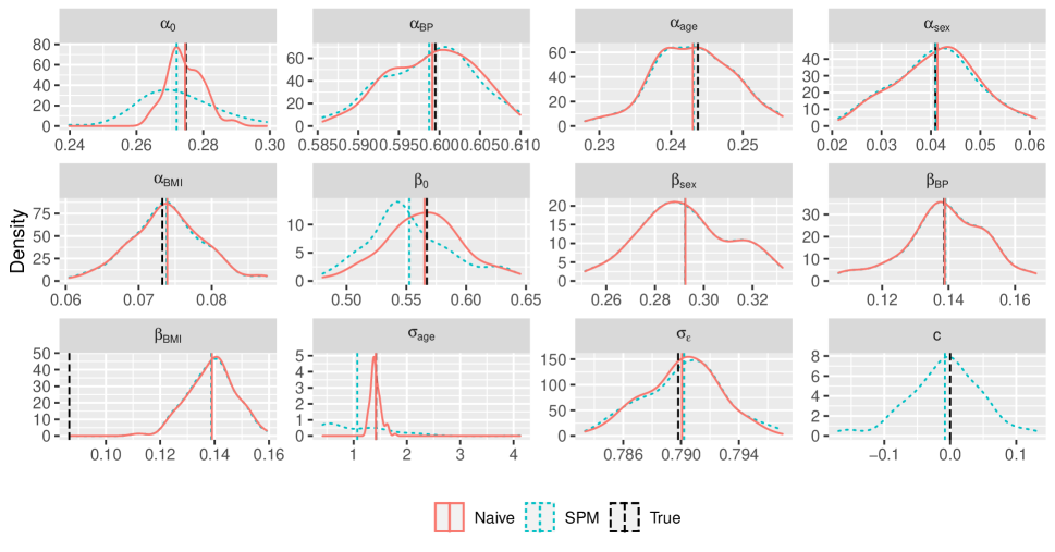
Figure 14: Distribution of posterior mean estimates on simulated data MAR following the SPM. The mean of posterior means for both the SPM and naive model and the true value are indicated by the vertical lines.

In this work, we propose reasonable models in the form of a shared parameter model (SPM) for predicting future blood pressure ($BP_{F}$) and missing status based on the HUNT Study accounting for missing data in the response. The SPM is compared to a naive model which assumes data MAR. There are some, but not massive, differences between the two models. Especially the effect of current blood pressure is larger in the SPM than the naive model. The simulation study confirms that if the underlying assumption of data following the SPM is valid, the SPM accounts for this better than the naive model. We note that there seem to be some issues resulting in a bias when the data is MNAR and a low coverage for some model parameters in the simulation studies (Figure 7, Figure 14, Table 8, and Table 9). This bias is especially pronounced for the association effect $c$ when the data is MNAR. Initially we suspected that the low coverage could be due to misspecification of the informative prior used for $c$. However, the prior sensitivity study presented in Supplementary material E indicates that the model is robust to prior specifications concerning the association parameter.

In this paper we have validated the models based on predictive performance based on a validation data set, both in straight forward predictive performance for the present participants and through the new validation scheme proposed in Section 3.5. The results indicate that missing status contains information about future blood pressure ($BP_{F}$) given the SPM. According to the simulation studies on this validation scheme (Section 5.2), the model predictions conditioned on missing status are only better than those without knowledge on missing status if data is MNAR (Figure 9). When the data is MAR, the mean absolute error of the two posterior mean predictions are almost identical. Hence, we have strong indications that blood pressure missing in the HUNT Study is MNAR.

As this research was motivated by the need of a predictive model of future blood pressure accounting for missing data, we performed all simulation studies related to bias, coverage and predictive performance on data sets that mimic our study system in size and explanatory variables, i.e. the HUNT2 cohort for training and the HUNT3 cohort for validation. Exploring asymptotic properties of the models and validation schemes or how uncertainty, biases and predictive performance change with the size of the datasets and missingness have been outside the scope of this work.

Driven by the results of this case study we find the properties of the validation schemes an interesting topic of further research. One approach would be to study the models and results of this work in the framework of missingness graphs introduced by Mohan and Pearl (2021) and the missing at random counterpart models of Molenberghs et al. (2008).

We acknowledge that the models presented in this work are non-trivial to set up and are computationally demanding. With the available code it is relatively straightforward to do inference and simulation studies for similar datasets. The quantity of interest do not need to follow a Gaussian likelihood, but can be any member of the exponential family.

7 Acknowledgement

The Trøndelag Health (HUNT) Study is a collaboration between HUNT Research Centre (Faculty of Medicine and Health Sciences, Norwegian University of Science and Technology NTNU), Trøndelag County Council, Central Norway Regional Health Authority, and the Norwegian Institute of Public Health. Participation in the HUNT Study is voluntary, and all participants provided written informed consent before participation. The Regional Committee on Medical and Health Research Ethics of Norway (REK; 2018/1824) approved this work in July 2021.

8 Funding

This work is sponsored by NTNU’s Digital Transformation project ’My Medical Digital Twin’.

Appendix A The Trøndelag Health Study Protocol

The HUNT Study protocols are described in detail by Krokstad et al. [2013] and Åsvold et al. [2021]. Here, we briefly overview the performed data collection relevant to this work. Age and sex were extracted from the Norwegian Population Registry. Height and weight were measured after removing shoes and other heavy clothing. Blood pressure was measured, by trained personnel, in a sitting position after two minutes of rest. Three measurements were taken, one minute apart, of which the mean of the second and third were used to report blood pressure. To assess the current use of blood pressure medication, self-reported questionnaires were used. In HUNT2, the current use captured in ”Are you taking medication for high blood pressure?” [Never; Previously; Currently]. In HUNT3, the question was reformulated to ”Do you take, or have you taken medication for high blood pressure?” [No; Yes]. Therefore, we combine this question with the answer to ”If you are currently taking medicine for high blood pressure, have you felt unwell/ had side effects from this medicine?”. We assume only the participant who currently takes medication answered this question. In HUNT4, the use of BP medicine was captured in ”Do you currently use any prescription medication for high blood pressure?” [No; Yes].

Appendix B Summary of the HUNT3 Cohort

The validation data set (HUNT3 cohort) consists of participants with observations of $BP$, $age$, $BMI$ and $sex$ in HUNT3, and $BP$ and missing status in HUNT4. Of $50201$ in HUNT3, $33.3\%$ drop out prior to HUNT4. Summary statistics for the HUNT3 cohort are given in Table 5, together with group mean for HUNT3 observations grouped on missing status.

Table 5: The sample mean and standard deviation of $BP_{F}$, $BP_{I}$, $age$, and $BMI$ and proportion of female/male participants in the HUNT3 cohort are displayed in the third column. The fourth and fifth columns displays sample mean for the present and missing participants in addition to proportions of present/missing participants for the whole cohort and per sex.

Summary of the HUNT3 cohort
Variable	Unit	HUNT3	Present in HUNT4	Missing in HUNT4,
$\text{BP}_{4}$	mmHg	-	136.48	-
$\text{BP}_{3}$	mmHg	133.21 (20.71)	131.48	136.67
$\text{age}_{3}$	years	53.08 (16.01)	51.68	55.90
$\text{BMI}_{3}$	kg/$m^{2}$	27.17 (4.41)	27.12	27.28
sex			66.7 %	33.3 %
female	0	54.6 %	68.7 %	31.3 %
male	1	45.4 %	64.3 %	35.7 %

Appendix C Shared Parameter Model With Additive Effects

Based on the work done by Espeland [2020] we explore the need for non-linear effects in the SPM introduced in Section 3.2. We model all continuous variables as additive effects ($f(z)$) through a random walk of order 2 with a sum to zero constraints [Gómez-Rubio, 2020]. Let $m=1:n$ be the index for the increments and define $\Delta^{2}z_{m}=z_{m}-2z_{m+1}+z_{m+2}\sim N(0,\sigma^{2})$. The density for $f(\boldsymbol{z})$ is, $f(\boldsymbol{z}|\sigma)\propto\sigma^{-\frac{n-2}{2}}exp\Bigg{\{}-\frac{1}{2\sigma}\sum_{m=1}^{n-2}(\Delta^{2}z_{m})\Bigg{\}}$. Further, the sum of all random effect components is constrained to be zero. For more information about random walk priors and sum to zero constraints, see Rue and Held [2005].

The specification of linear predictors of the SPM defined in Section 3.2 becomes,

$$\eta_{BPi}=\alpha_{0}+f_{BP_{F}}({BP_{I}}_{i})+f_{BP_{F}}(age_{i})+f_{BP_{F}}({BMI}_{i})+\alpha_{sex}sex_{i}+{\epsilon}_{i}$$ (4)

$$\eta_{mi}=\beta_{0}+f_{m}({BP_{I}}_{i})+f_{m}(age_{i})+f_{m}({BMI}_{i})+\beta_{sex}sex_{i}+c{\epsilon}_{i}.$$

All regression parameters $\alpha_{0}$, $\alpha_{sex}$, $\beta_{0}$, and $\beta_{sex}$ are given independent priors $N(0,{10^{3}}^{2})$. The shared parameters $\epsilon_{i}$ are assumed to be independent Gaussian $\epsilon_{i}\sim N(0,\sigma_{\epsilon}^{2})$. Both the additive effects $f(.)$ and ${\epsilon}_{i}$ have hyperparameters (${\sigma_{BP_{F}}}_{BP_{I}}$, ${\sigma_{BP_{F}}}_{age}$, ${\sigma_{BP_{F}}}_{BMI}$, ${\sigma_{m}}_{BP_{I}}$, ${\sigma_{m}}_{age}$, ${\sigma_{m}}_{BMI}$, $\sigma_{{\epsilon}}$) with independent gamma priors, $\text{Gamma}(1,5\cdot 10^{5})$. The association parameter $c$ is given an informative prior $c\sim N(0,1^{2})$.

Modeling all parameters in an additive way is computationally demanding. With 32 CPU cores and 32 GB memory, we were still only able to fit the SPM 4 with $15000$ ($\approx 25\%$) participants. These participants were drawn randomly. The results are given in Figure 11. The age effect in the missing process is clearly non-linear. The other continuous variables, although not perfectly linear, are much closer to being linear.

Therefore, we chose to model all variables linearly except for age in the dropout process, which we model as an additive effect.

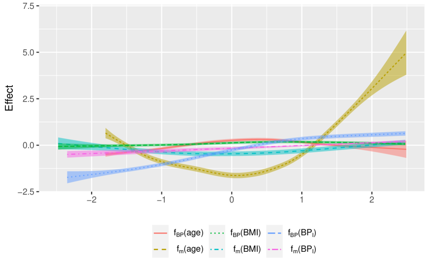
Figure 11: Additive effects of $age$, $BMI$, and $BP_{I}$ in the SPM for both the $BP$ process and the missing process fitted on 15000 randomly drawn participants from the HUNT2 cohort.

Appendix D Parameter estimates

The parameter estimates from the SPM and naive model introduces in Section 3.2 fitted on the HUNT2 cohort, together with their $95\%$ equitailed credible intervals model are presented in Table 6.

Table 6: Summary of all parameters estimated for both the SPM and the naive model fitted on teh HUNT2 cohort. The posterior means and $95\%$ credible intervals are displayed.

	SPM		Naive
	Posterior mean	CI	Posterior mean	CI
$\alpha_{0}$	0.275	(0.259, 0.291)	0.134	(0.123, 0.145)
$\alpha_{age}$	0.244	(0.232, 0.255)	0.246	(0.235, 0.258)
$\alpha_{BMI}$	0.073	(0.064, 0.082)	0.071	(0.062, 0.080)
$\alpha_{BP}$	0.599	(0.589, 0.610)	0.578	(0.567, 0.588)
$\alpha_{sex}$	0.041	(0.025, 0.057)	-0.022	(-0.064, 0.019)
$\beta_{0}$	0.567	(0.475, 0.666)	0.55	(0.460, 0.651)
$\beta_{BMI}$	0.087	(0.087, 0.106)	0.081	(0.063, 0.099)
$\beta_{BP}$	0.139	(0.139, 0.162)	0.133	(0.111, 0.155)
$\beta_{sex}$	0.292	(0.292, 0.329)	0.275	(0.240, 0.310)
$\sigma_{age}$	1.412	(0.946, 2.130)	1.400	(0.927, 2.123)
$\sigma_{\epsilon}$	0.790	(0.783, 0.797)	0.77	(0.765, 0.776)
c	0.705	(0.645, 0.765)	-	-

Appendix E Prior Sensitivity Analysis

Model name	$c\_0\_1$	$c\_0\_10$	$c\_0\_100$	$c\_1\_1$	$c\_1\_10$	$c\_1\_100$	$c\_10\_100$
Prior for c	N(0,$1^{2}$)	N(0,$10^{2}$)	N(0,$100^{2}$)	N(1,$1^{2}$)	N(1,$10^{2}$)	N(1,$100^{2}$)	N(10,$100^{2}$)

Table 7: Priors for association parameter c.

As the SPM model specified in Section 3.2 is rather complex, we perform a sensitivity analysis to evaluate if the model is sensitive to the choice of prior for the association parameter $c$ (3). This parameter is of special interest as it defines the connection between the dropout process and the measurements process, $BP_{F}$. We fit the model defined in (3) with different choices for the prior for $c$ displayed in Table 7.

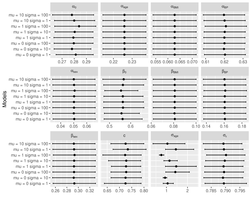
Figure 12: Posterior mean and 95% credible intervals for all parameters of the SPM with different priors for the association parameter $c$. The model names are constructed so the first digit is the mean and the second the is the standard deviation used in the prior for c.

Figure 12 shows the resulting $95\%$ equi-tailed credible intervals for all parameters. We clearly see that the latent field, $\alpha_{0}$, $\alpha_{BP}$, $\alpha_{age}$, $\alpha_{BMI}$, $\alpha_{sex}$, $\beta_{0}$, $\beta_{BP}$, $\beta_{BMI}$, $\beta_{sex}$, have almost identical credible intervals. The credible intervals for the hyperparameter $\sigma_{age}$ vary slightly more. However, we see in Figure 13 that the resulting posterior mean of the age effect is practically identical for all the different priors. Hence we conclude that the model is not sensitive to different choices of $c$.

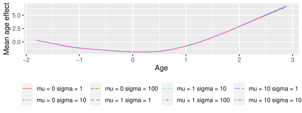
Figure 13: Mean posterior age effect for all models tested in the prior sensitivity study.

Appendix F Supplementary Material for The Simulation Studies on Bias and Coverage

We have summarized the results from the simulation study performed in Section 5.1 exploring the bias and coverage of the SPM and the naive model. In addition, we have performed a similar study with data MAR. The distribution of the posterior means from the simulation study when the true parameters are the posterior mean estimates of the SPM and the data is MAR can be seen in Figure 7. Table 8, and Table 9 display the mean posterior mean, bias, and coverage of the parameter estimates for both the SPM and the naive model for simulated data MNAR and MAR, respectively. Further we display the difference in bias for the SPM and naive model $Bias_{SPM}-Bias_{naive}$ also in Table 8, and Table 9.

Table 8: A summary of the results where we explore the bias and coverage of the SPM and the naive mode when the true model parameters are known. We display the mean posterior mean, bias of posterior means, and coverage for all parameters. In addition, we display the difference in bias for the SPM and the naive model ($Bias_{SPM}-Bias_{naive}$). The true parameters are the posterior means from the SPM as given in Table 6 and the data is MNAR.

		SPM			Naive model
	True value	Mean	Bias	Coverage	Mean	Bias	Coverage	Difference in bias
$\alpha_{0}$	0.27	0.24	-3e-02	0.07	0.13	-0.144	0.00	0.112
$\alpha_{BP}$	0.60	0.60	-4e-03	0.91	0.58	-0.021	0.01	0.017
$\alpha_{age}$	0.24	0.24	-8e-04	0.98	0.25	0.002	0.97	0.001
$\alpha_{bmi}$	0.07	0.07	-1e-03	0.95	0.07	-0.006	0.76	0.004
$\alpha_{sex}$	0.04	0.04	-3e-03	0.97	0.02	-0.018	0.42	0.015
$\beta_{0}$	0.57	0.56	-1e-02	0.98	0.55	-0.016	0.99	0.004
$\beta_{BMI}$	0.09	0.13	5e-02	0.01	0.13	0.042	0.01	-0.005
$\beta_{sex}$	0.29	0.29	-5e-03	0.93	0.28	-0.016	0.86	0.011
$\beta_{BP}$	0.14	0.14	-3e-03	0.90	0.13	-0.007	0.91	0.004
$\sigma_{age}$	1.42	1.22	-2e-01	0.67	1.34	-0.082	1.00	-0.119
$\sigma_{\epsilon}$	0.79	0.78	-8e-03	0.32	0.77	-0.020	0.00	0.012
$c$	0.70	0.55	-2e-01	0.00	NA	NA	NA	NA

Table 9: A summary of the results where we explore the bias and coverage of the SPM and the naive model when the true model parameters are known. We display the mean posterior mean, bias of posterior means, and coverage for all parameters. Further, we display the difference in bias for the SPM and the naive model ($Bias_{SPM}-Bias_{naive}$). The true parameters are the posterior means from the SPM as given in Table 6 and the data is MAR meaning $c=0$.

		SPM			Naive model
	True value	Mean	Bias	Coverage	Mean	Bias	Coverage	Difference in bias
$\alpha_{0}$	0.27	0.272	-3e-03	0.8	0.27	-2e-04	1.0	-3e-03
$\alpha_{BP}$	0.60	0.599	-8e-04	1.0	0.60	-4e-04	1.0	-4e-04
$\alpha_{age}$	0.24	0.243	-6e-04	1.0	0.24	-7e-04	1.0	1e-04
$\alpha_{bmi}$	0.07	0.074	6e-04	0.9	0.07	7e-04	0.9	1e-04
$\alpha_{sex}$	0.04	0.041	7e-05	0.9	0.04	4e-04	1.0	4e-04
$\beta_{0}$	0.57	0.553	-1e-02	1.0	0.57	-2e-03	1.0	-1e-02
$\beta_{BMI}$	0.09	0.139	5e-02	0.0	0.14	5e-02	0.0	2e-04
$\beta_{sex}$	0.29	0.292	-4e-05	0.9	0.29	9e-05	0.9	4e-05
$\beta_{BP}$	0.14	0.139	3e-04	0.9	0.14	2e-04	0.9	-1e-04
$\sigma_{age}$	1.42	1.069	-4e-01	0.4	1.41	-6e-03	1.0	-3e-01
$\sigma_{\epsilon}$	0.79	0.790	4e-04	1.0	0.79	3e-04	1.0	-1e-04
$c$	0.00	-0.008	-8e-03	0.9	NA	NA	NA	NA

References

- Albert and Follmann [2000] Paul S Albert and Dean A Follmann. Modeling repeated count data subject to informative dropout. Biometrics, 56(3):667–677, 2000.
- Anderson Jr et al. [1994] Gunnar H Anderson Jr, Nancy Blakeman, and DH Streeten. The effect of age on prevalence of secondary forms of hypertension in 4429 consecutively referred patients. Journal of hypertension, 12(5):609–615, 1994.
- Åsvold et al. [2021] Bjørn Olav Åsvold, Arnulf Langhammer, Tommy Aune Rehn, Grete Kjelvik, Trond Viggo Grøntvedt, Elin Pettersen Sørgjerd, Jørn Søberg Fenstad, Oddgeir Holmen, Maria C Stuifbergen, Sigrid Anna Aalberg Vikjord, et al. Cohort profile update: The hunt study, norway. medRxiv, 2021.
- Balakrishnan [2009] Narayanaswamy Balakrishnan. Methods and applications of statistics in the life and health sciences. John Wiley & Sons, 2009.
- Brown et al. [2000] Clarice D Brown, Millicent Higgins, Karen A Donato, Frederick C Rohde, Robert Garrison, Eva Obarzanek, Nancy D Ernst, and Michael Horan. Body mass index and the prevalence of hypertension and dyslipidemia. Obesity research, 8(9):605–619, 2000.
- Creemers et al. [2010] An Creemers, Niel Hens, Marc Aerts, Geert Molenberghs, Geert Verbeke, and Michael G Kenward. A sensitivity analysis for shared-parameter models for incomplete longitudinal outcomes. Biometrical Journal, 52(1):111–125, 2010.
- Diggle and Kenward [1994] Peter Diggle and Michael G Kenward. Informative drop-out in longitudinal data analysis. Journal of the Royal Statistical Society: Series C (Applied Statistics), 43(1):49–73, 1994.
- Enders [2011] Craig K Enders. Missing not at random models for latent growth curve analyses. Psychological methods, 16(1):1, 2011.
- Espeland [2020] Lars Fredrik Espeland. A shared parameter model accounting for non-ignorable missing data due to dropout: Modelling of blood pressure based on the hunt study. Master’s thesis, Norwegian University of Science and Technology, 7 2020.
- Fahrmeir et al. [2007] Ludwig Fahrmeir, Thomas Kneib, Stefan Lang, and Brian Marx. Regression. Springer, 2007.
- Follmann and Wu [1995] Dean Follmann and Margaret Wu. An approximate generalized linear model with random effects for informative missing data. Biometrics, 51(1):151–168, 1995.
- Gad and Darwish [2013] Ahmed M Gad and Nesma MM Darwish. A shared parameter model for longitudinal data with missing values. American journal of applied Mathematics and Statistics, 1(2):30–35, 2013.
- GitHub [2021] GitHub. A-spm-accounting-for-data-mnar, 2021. URL https://github.com/AuroraSmil/A-SPM-accounting-for-data-MNAR.
- Gneiting and Raftery [2007] Tilmann Gneiting and Adrian E Raftery. Strictly proper scoring rules, prediction, and estimation. Journal of the American statistical Association, 102(477):359–378, 2007.
- Gómez-Rubio [2020] Virgilio Gómez-Rubio. Bayesian inference with INLA. Chapman & Hall/CRC Press. Boca Raton, FL., 2020.
- Griswold et al. [2021] Michael E Griswold, Rajesh Talluri, Xiaoqian Zhu, Dan Su, Jonathan Tingle, Rebecca F Gottesman, Jennifer Deal, Andreea M Rawlings, Thomas H Mosley, B Gwen Windham, and Karen Bandeen-Roche5. Reflection on modern methods: shared-parameter models for longitudinal studies with missing data. International journal of epidemiology vol. 50,4 (2021): 1384-1393. doi:10.1093/ije/dyab086, 50(4):1384–1393, 2021.
- Heckman [1979] James J Heckman. Sample selection bias as a specification error. Econometrica: Journal of the econometric society, 47(1):153–161, 1979.
- Henderson et al. [2000] Robin Henderson, Peter Diggle, and Angela Dobson. Joint modelling of longitudinal measurements and event time data. Biostatistics, 1(4):465–480, 2000.
- Howe et al. [2016] Chanelle J Howe, Stephen R Cole, Bryan Lau, Sonia Napravnik, and Joseph J Eron Jr. Selection bias due to loss to follow up in cohort studies. Epidemiology (Cambridge, Mass.), 27(1):91, 2016.
- Jiang et al. [2016] Shu-Zhong Jiang, Wen Lu, Xue-Feng Zong, Hong-Yun Ruan, and Yi Liu. Obesity and hypertension. Experimental and therapeutic medicine, 12(4):2395–2399, 2016.
- Kaciroti and Little [2021] Niko A Kaciroti and Roderick JA Little. Bayesian sensitivity analyses for longitudinal data with dropouts that are potentially missing not at random: A high dimensional pattern-mixture mode. Statistics in Medicine, 40(21):4609–4628, 2021.
- Krokstad et al. [2013] S Krokstad, A Langhammer, K Hveem, TL Holmen, K Midthjell, TR Stene, G Bratberg, J Heggland, and J Holmen. Cohort profile: the hunt study, norway. International journal of epidemiology, 42(4):968–977, 2013.
- Lewington et al. [2002] Lewington et al. Age-specific relevance of usual blood pressure to vascular mortality: a meta-analysis of individual data for one million adults in 61 prospective studies. The Lancet, 360(9349):1903–1913, 2002.
- Linero and Daniels [2018] Antonio R Linero and Michael J Daniels. Bayesian approaches for missing not at random outcome data: The role of identifying restrictions. Statistical science: a review journal of the Institute of Mathematical Statistics, 33(2):198, 2018.
- Little [1993] Roderick JA Little. Pattern-mixture models for multivariate incomplete data. Journal of the American Statistical Association, 88(421):125–134, 1993.
- Little [1995] Roderick JA Little. Modeling the drop-out mechanism in repeated-measures studies. Journal of the american statistical association, 90(431):1112–1121, 1995.
- Little and Rubin [2019] Roderick JA Little and Donald B Rubin. Statistical analysis with missing data, volume 793. John Wiley & Sons, 2019.
- Martino and Riebler [2019] Sara Martino and Andrea Riebler. Integrated nested laplace approximations (inla). Wiley StatsRef: Statistics Reference Online, pages 1–19, 2019.
- Mohan and Pearl [2021] Karthika Mohan and Judea Pearl. Graphical models for processing missing data. Journal of the American Statistical Association, 116(534):1023–1037, 2021.
- Molenberghs et al. [2008] Geert Molenberghs, Caroline Beunckens, Cristina Sotto, and Michael G Kenward. Every missingness not at random model has a missingness at random counterpart with equal fit. Journal of the Royal Statistical Society: Series B (Statistical Methodology), 70(2):371–388, 2008.
- Murray et al. [2020] Christopher JL Murray, Aleksandr Y Aravkin, Peng Zheng, Cristiana Abbafati, Kaja M Abbas, Mohsen Abbasi-Kangevari, Foad Abd-Allah, Ahmed Abdelalim, Mohammad Abdollahi, Ibrahim Abdollahpour, et al. Global burden of 87 risk factors in 204 countries and territories, 1990–2019: a systematic analysis for the global burden of disease study 2019. The Lancet, 396(10258):1223–1249, 2020.
- Pulkstenis et al. [1998] Erik P Pulkstenis, Thomas R Ten Have, and J Richard Landis. Model for the analysis of binary longitudinal pain data subject to informative dropout through remedication. Journal of the American Statistical Association, 93(442):438–450, 1998.
- R-INLA [2021] R-INLA. R-inla project, 2021. URL https://www.r-inla.org/home.
- Rapsomaniki et al. [2014] Eleni Rapsomaniki, Adam Timmis, Julie George, Mar Pujades-Rodriguez, Anoop D Shah, Spiros Denaxas, Ian R White, Mark J Caulfield, John E Deanfield, Liam Smeeth, et al. Blood pressure and incidence of twelve cardiovascular diseases: lifetime risks, healthy life-years lost, and age-specific associations in 1· 25 million people. The Lancet, 383(9932):1899–1911, 2014.
- Rhoads [2012] Christopher H Rhoads. Problems with tests of the missingness mechanism in quantitative policy studies. Statistics, Politics, and Policy, 3(1), 2012.
- Rue and Held [2005] Havard Rue and Leonhard Held. Gaussian Markov random fields: theory and applications. CRC press, 2005.
- Rue et al. [2009] Håvard Rue, Sara Martino, and Nicolas Chopin. Approximate bayesian inference for latent gaussian models by using integrated nested laplace approximations. Journal of the royal statistical society: Series b (statistical methodology), 71(2):319–392, 2009.
- Rue et al. [2017] Håvard Rue, Andrea Riebler, Sigrunn H Sørbye, Janine B Illian, Daniel P Simpson, and Finn K Lindgren. Bayesian computing with inla: a review. Annual Review of Statistics and Its Application, 4:395–421, 2017.
- Steinsland et al. [2014] Ingelin Steinsland, Camilla Thorrud Larsen, Alexandre Roulin, and Henrik Jensen. Quantitative genetic modeling and inference in the presence of nonignorable missing data. Evolution, 68(6):1735–1747, 2014.
- Thomas et al. [1998] R Thomas, Ten Have, Allen R Kunselman, Erik P Pulkstenis, and J Richard Landis. Mixed effects logistic regression models for longitudinal binary response data with informative drop-out. Biometrics, 54(1):367–383, 1998.
- Tobin et al. [2005] Martin D Tobin, Nuala A Sheehan, Katrina J Scurrah, and Paul R Burton. Adjusting for treatment effects in studies of quantitative traits: antihypertensive therapy and systolic blood pressure. Statistics in medicine, 24(19):2911–2935, 2005.
- Tozawa et al. [2003] Masahiko Tozawa, Kunitoshi Iseki, Chiho Iseki, Kozen Kinjo, Yoshiharu Ikemiya, and Shuichi Takishita. Blood pressure predicts risk of developing end-stage renal disease in men and women. Hypertension, 41(6):1341–1345, 2003.
- Vonesh et al. [2006] Edward F Vonesh, Tom Greene, and Mark D Schluchter. Shared parameter models for the joint analysis of longitudinal data and event times. Statistics in medicine, 25(1):143–163, 2006.
- Whelton [1994] Paul K Whelton. Epidemiology of hypertension. Lancet (London, England), 344(8915):101–106, 1994.
- World Health Organizatoin [2013] World Health Organizatoin. Global action plan for the prevention and control of ncds 2013-2020, 2013. URL https://www.who.int/publications/i/item/9789241506236.
- Wu and Carroll [1988] Margaret C Wu and Raymond J Carroll. Estimation and comparison of changes in the presence of informative right censoring by modeling the censoring process. Biometrics, 44(1):175–188, 1988.
- Zhou et al. [2017] Bin Zhou, James Bentham, Mariachiara Di Cesare, Honor Bixby, Goodarz Danaei, Melanie J Cowan, Christopher J Paciorek, Gitanjali Singh, Kaveh Hajifathalian, James E Bennett, et al. Worldwide trends in blood pressure from 1975 to 2015: a pooled analysis of 1479 population-based measurement studies with 19· 1 million participants. The Lancet, 389(10064):37–55, 2017.