Autonomous Navigation of AGVs in Unknown Cluttered Environments: log-MPPI Control Strategy

Abstract

Sampling-based model predictive control (MPC) optimization methods, such as Model Predictive Path Integral (MPPI), have recently shown promising results in various robotic tasks. However, it might produce an infeasible trajectory when the distributions of all sampled trajectories are concentrated within high-cost even infeasible regions. In this study, we propose a new method called log-MPPI equipped with a more effective trajectory sampling distribution policy which significantly improves the trajectory feasibility in terms of satisfying system constraints. The key point is to draw the trajectory samples from the normal log-normal (NLN) mixture distribution, rather than from Gaussian distribution. Furthermore, this work presents a method for collision-free navigation in unknown cluttered environments by incorporating the 2D occupancy grid map into the optimization problem of the sampling-based MPC algorithm. We first validate the efficiency and robustness of our proposed control strategy through extensive simulations of 2D autonomous navigation in different types of cluttered environments as well as the cartpole swing-up task. We further demonstrate, through real-world experiments, the applicability of log-MPPI for performing a 2D grid-based collision-free navigation in an unknown cluttered environment, showing its superiority to be utilized with the local costmap without adding additional complexity to the optimization problem. A video demonstrating the real-world and simulation results is available at https://youtu.be/_uGWQEFJSN0.

I Introduction and Related Work

Designing a safe, reliable, and robust control methodology for autonomous navigation of autonomous ground vehicles (AGVs) in unknown cluttered environments (such as dense forests, crowded offices, corridors, warehouses, etc.) has been known as a great challenge. Such a navigation task requires the AGV to navigate safely with full autonomy while avoiding getting trapped in local minima and collision with static and dynamic obstacles while moving towards the goal, as well as respecting various system constraints. To this end, the robot should be capable of perceiving its surrounding environment and then reacting adequately. This subsequently results in a complex optimization control problem that is difficult to be solved in real-time [1].

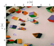
(a)

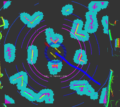
(b)

Figure 1: Snapshot of (a) our Jackal robot equipped with a Velodyne VLP-16 LiDAR and located in an unknown cluttered environment ($G_{1},\dots,G_{4}$: desired poses), and (b) the corresponding 2D local costmap that represents the surrounding obstacles, where purple and cyan cells represent obstacles and their inflation, respectively; while blue line is the planned trajectory by our log-MPPI control strategy.

One of the well-established and promising control strategies for collision-free navigation is Model Predictive Control (MPC) strategy, owing to its flexibility and ability to compute good control policy in the presence of the hard and soft constraints of the system to be controlled. It leverages a receding horizon strategy to plan a sequence of optimal control inputs over a prediction time-horizon; then, the first control input in the sequence is applied to the system, while the remaining control sequence is used for warm-starting the optimization at the next time-step [2]. The existing MPC-based schemes can be mainly categorized into gradient-based and sampling-based trajectory optimization methods. The gradient-based MPC methods have been successfully applied to real robotic systems, obtaining smooth collision-free trajectories in the presence of obstacles and other constraints [3, 4, 5, 6]. However, the gradient-based frameworks are typically based on strong assumptions: the cost function, and sometimes system constraints, need to be differentiable in order to leverage the gradient for computing the optimal solution. Unfortunately, in practice, the optimization problem often involves non-convex and non-differentiable objective function with discontinuous collision avoidance constraints, and it can be computationally difficult to be solved in real-time. To alleviate these issues, for example, the non-differentiable system constraints can be reformulated into smooth and differentiable ones as presented in [7]. A promising alternative is the sampling-based optimization methods such as Model Predictive Path Integral (MPPI) control strategy [8] that (i) makes no assumptions or approximations on the objective functions and system dynamics, (ii) can be effectively applied on highly dynamic systems, and (iii) benefits from the parallel nature of sampling and high computational capacities of Graphics Processing Units (GPUs) utilized for speeding up the optimization.

Recently, MPPI or sampling-based MPC has been successfully applied to a wide variety of robotic applications, starting from aggressive driving [9, 10] and autonomous flight [1, 11] and ending with visual servoing [12] and reactive manipulation [13], showing outstanding performance in the presence of non-convex and discontinuous objectives, without adding any additional complexity to the optimization problem. Despite the attractive characteristics of MPPI [14], much like any sampling-based optimization method, it might generate an infeasible control sequence (i.e., infeasible trajectory) when the distributions of all sampled trajectories drawn from the system dynamics are unfortunately surrounding some infeasible region. This may inevitably lead to either violating the system constraints or increasing the risk of being trapped in local minima. For tasks such as collision-free navigation in cluttered environments, it has been observed that the collisions may not be avoided, as the intensive simulations demonstrated in Section IV. To mitigate this problem, authors in [15] employed an iterative Linear Quadratic Gaussian (iLQG) control, as an ancillary controller, on top of MPPI for tracking the planned trajectory. Similarly, in [16], MPPI is augmented with a nonlinear $\mathcal{L}_{1}$ adaptive controller to compensate for the model uncertainty. Lately, the covariance steering (CS) principle is incorporated within the MPPI algorithm, aiming to introduce adjustable trajectory sampling distributions [17]. However, the proposed solutions in [16] and [17] have not been experimentally validated on real robotic systems.

With the aim of mitigating the previous shortcomings and improving the performance of MPPI, we propose a new strategy, called log-MPPI control strategy, that provides more flexible and efficient distributions of the sampled trajectories, without the need for (i) integrating an ancillary controller on top of MPPI [16, 15], or (ii) adding a feedback term along with the injected artificial noise that requires the system dynamics to be linearized and converts the original optimization problem into a convex one [17]. The key idea of log-MPPI is that the trajectories (or, the control input updates) are sampled from the product of normal and log-normal distribution (namely, NLN mixture), instead of sampling from only Gaussian distribution. With such a sampling strategy, a small injected noise variance can be utilized so that violating system constraints can be avoided; yet, we can still get desirable sampled rollout trajectories that are well spread-out for covering large state-space. In summary, the contributions of this work can be summarized as follows:

1. We provide a new sampling strategy based on normal log-normal mixture distribution. This new sampling method provides more efficient trajectories than the vanilla MPPI variants, ensuring a much better exploration of the state-space of the given system and reducing the risk of getting stuck in local minima, leading the robot to ultimately find feasible trajectories that avoid collision, as revealed in Section IV-B.

2. Then, we show through the cartpole swing-up task given in Section IV-A the robustness of log-MPPI to run with a significantly fewer number of trajectories, opening up a new avenue for the sampling-based MPC algorithm to be run on a standard CPU instead of a GPU. We thereafter incorporate the 2D grid map, as a local costmap, into the sampling-based MPC algorithm for performing collision-free navigation in either static or dynamic unknown cluttered environments, as depicted in Section IV-C.

3. Finally, in Section V, we experimentally demonstrate our control strategy for a 2D grid-based navigation in an unknown indoor cluttered environment shown in Fig. 1; to the best of the authors’ knowledge, this is the first attempt to experimentally achieve grid-based collision-free navigation based on sampling-based MPC.

II Preliminaries

In this section, we define the optimal control problem to be solved and provide a brief review of MPPI.

II-A Constrained Control Problem

Consider a discrete-time system with state $\mathbf{x}_{k}\in\mathbb{R}^{n}$, control input $\mathbf{u}_{k}\in\mathbb{R}^{m}$, and underlying dynamics $\mathbf{x}_{k+1}=f\left(\mathbf{x}_{k},\mathbf{v}_{k}\right)$. Let $\mathbf{v}_{k}=\mathbf{u}_{k}+\delta\mathbf{u}_{k}\sim\mathcal{N}(\mathbf{u}_{k},\Sigma_{\mathbf{u}})$ where $\delta\mathbf{u}_{k}\sim\mathcal{N}(\mathbf{0},\Sigma_{\mathbf{u}})$ represents the injected disturbance with a zero-mean and co-variance $\Sigma_{\mathbf{u}}$. Let $\mathbf{U}=\left(\mathbf{u}_{0},\mathbf{u}_{1},\dots,\mathbf{u}_{N-1}\right)\in\mathbb{R}^{m\times N}$ denote the control sequence over a finite time-horizon $N$, while $\mathbf{X}=\left(\mathbf{x}_{0},\mathbf{x}_{1},\dots,\mathbf{x}_{N-1}\right)\in\mathbb{R}^{n\times N}$ denotes the resulting state trajectory. Let $\mathcal{O}^{\text{rob}}\left(\mathbf{x}_{k}\right)$ and $\mathcal{O}^{\text{obs}}$ be the area occupied by the robot and the obstacles, respectively. Our objective is to find a control sequence $\mathbf{U}$ that generates a collision-free trajectory which allows the robot to navigate from the initial state $\mathbf{x}_{s}$ to its desired state $\mathbf{x}_{f}$ while minimizing a cost function $J$. This optimization problem can be formulated by MPPI as:

$$\min_{\mathbf{U}}\quad J =\mathbb{E}\left[\phi\left(\mathbf{x}_{N}\right)+\sum_{k=0}^{N-1}\left(q\left(\mathbf{x}_{k}\right)+\frac{1}{2}\mathbf{u}_{k}^{T}R\mathbf{u}_{k}\right)\right]\!,$$ (1a)

s.t. $$\mathbf{x}_{k+1}=f\left(\mathbf{x}_{k},\mathbf{v}_{k}\right),$$ (1b)

$$\mathcal{O}^{\text{rob}}\left(\mathbf{x}_{k}\right)\cap\mathcal{O}^{\text{obs}}=\emptyset,\;\mathbf{h}(\mathbf{x}_{k},\mathbf{u}_{k})\leq 0,$$ (1c)

$$\mathbf{x}_{0}=\mathbf{x}_{s},\;\mathbf{u}_{k}\in\mathbf{U},\;\mathbf{x}_{k}\in\mathbf{X},$$ (1d)

where $\phi\left(\mathbf{x}_{N}\right)$, $q\left(\mathbf{x}_{k}\right)$, and $R\in\mathbb{R}^{m\times m}$ denote the terminal cost, state-dependent running cost, and positive definite control weighting matrix, respectively. MPPI solves the problem by minimizing the objective (1a) subject to system dynamics (1b) and system constraints such as collision avoidance and control constraints (1c).

II-B Review of MPPI

Unlike the gradient-based MPC methods, MPPI does not compute gradients to find the optimal solution; i.e., it is a derivative-free trajectory optimization strategy. Moreover, it makes no assumptions on the objective functions and system dynamics; i.e., highly nonlinear and non-convex functions can be easily employed. At each time-step, MPPI draws $M$ trajectories, in parallel, from the system dynamics using GPU ensuring a real-time performance. These parallel trajectories are then evaluated according to its expected cost. The cost-to-go of each rollout $\tau$ over a time-horizon $N$ is given by

$$\vspace*{-4pt}\tilde{S}\left(\tau\right)=\phi\left(\mathbf{x}_{N}\right)+\sum_{k=0}^{N-1}\tilde{q}\left(\mathbf{x}_{k},\mathbf{u}_{k},\delta\mathbf{u}_{k}\right),$$ (2)

where $\tilde{q}\left(\mathbf{x}_{k},\mathbf{u}_{k},\delta\mathbf{u}_{k}\right)$ refers to the instantaneous running cost which consists of the sum of state-dependent running cost $q\left(\mathbf{x}_{k}\right)$ and quadratic control cost; it is defined as [8]

$$\tilde{q}\!=\!\underbrace{\vphantom{\frac{\left(1\!-\!\frac{1}{\nu}\right)}{2}\delta\mathbf{u}_{k}^{T}R\delta\mathbf{u}_{k}+\mathbf{u}_{k}^{T}R\delta\mathbf{u}_{k}+\frac{1}{2}\mathbf{u}_{k}^{T}R\mathbf{u}_{k}}q\left(\mathbf{x}_{k}\!\right)}_{\text{\color[rgb]{0,0,0}{{State-dep.}}}}\!+\!\underbrace{\frac{\left(1\!-\!\nu^{-1}\right)}{2}\delta\mathbf{u}_{k}^{T}R\delta\mathbf{u}_{k}\!+\!\mathbf{u}_{k}^{T}R\delta\mathbf{u}_{k}\!+\!\frac{1}{2}\mathbf{u}_{k}^{T}R\mathbf{u}_{k}}_{\text{\color[rgb]{0,0,0}{{Quadratic Control Cost}}}},$$ (3)

where $\nu\in\mathbb{R}^{+}$ determines how aggressively the state-space is explored. Afterwards, the control sequence is updated based on a weighted average cost over all sampled trajectories. As described in [8], the optimal control sequence $\left\{\mathbf{u}_{k}\right\}_{k=0}^{N-1}$ can be approximated as

$$\mathbf{u}_{k+1}=\mathbf{u}_{k}+\frac{\sum_{m=1}^{M}\exp\left(-(1/\lambda)\tilde{S}\left(\tau_{k,m}\right)\right)\delta\mathbf{u}_{k,m}}{\sum_{m=1}^{M}\exp\left(-(1/\lambda)\tilde{S}\left(\tau_{k,m}\right)\right)},$$ (4)

where $\tilde{S}\left(\tau_{k,m}\right)\in\mathbb{R}^{+}$ is the cost-to-go of the $m^{th}$ trajectory at $k^{th}$ step and $\lambda\in\mathbb{R}^{+}$ is so-called the inverse temperature which determines how selective the weighted average of the trajectories is [10]. The control sequence is then smoothed using a Savitzky-Galoy (SG) filter. Finally, the first control $\mathbf{u}_{0}$ in the sequence is applied to the system, while the remaining control sequence of length $N-1$ is used for warm-starting the optimization at the next time-step.

III log-MPPI Control Strategy

Our goal is to design a new sampling and control approach, the log-MPPI, to further improve the classic MPPI performance. Here, we briefly describe the difference between MPPI and log-MPPI: as previously discussed in Section II, MPPI does not update the injected control noise variance $\Sigma_{\mathbf{u}}$, and the state-space exploration is carried out by adjusting $\nu$ (see Eq. (3)). However, if $\nu$ is too large, MPPI produces control inputs with significant chatter [8]. Similarly, as stated in [15], a higher value of $\Sigma_{\mathbf{u}}$ might result in violating the system constraints and eventually state diverging. One solution could be updating, at each iteration, the variance [13]. Instead, we inject the log-normal along with normal distribution ensuring much better state exploration with a low variance value which well respects the system constraints and providing better performance with a fewer number of samples.

III-A Log-normal Distribution

In probability theory, a positive random variable $X$ is log-normally distributed, i.e., $X\sim\mathcal{LN}(\mu,\sigma^{2})$, if the natural logarithm of $X$ has a normal distribution with mean $\mu$ and variance $\sigma^{2}$, i.e., $\ln X\sim\mathcal{N}(\mu,\sigma^{2})$. Thus, the probability density function (pdf) of the random variable $X$ is given by

$$f_{X}(x)=\frac{1}{x\sigma\sqrt{2\pi\,}}\exp\left(-\frac{(\ln x-\mu)^{2}}{2\sigma^{2}}\right),x\in\mathbb{R}^{+},$$ (5)

where the mean and variance of a $\mathcal{LN}(\mu,\sigma^{2})$ distribution are given by

$$\mathbb{E}(X)=e^{(\mu+0.5\sigma^{2})}\;\text{and}\;\operatorname{Var}(X)=e^{(2\mu+\sigma^{2})}(e^{\sigma^{2}}-1).$$ (6)

In spite of the fact that both normal and log-normal distributions are unbounded distributions, the log-normal distribution is asymmetric and positively skewed to the right, where the range of values lies in an interval of $[0,+\infty[$. Therefore, the pdf, $f_{X}(x)$, starts at zero and increases to its mode, then decreases thereafter. The degree of skewness increases as $\sigma$ increases, for a given $\mu$. Similarly, for the same $\sigma$, the pdf’s skewness increases as $\mu$ increases. In addition, the most attractive feature of such distribution compared to the alternative default distributions (such as normal, gamma, and Weibull distributions) is its capability of capturing a large range with a long right-tail, making it convenient to model large values and hence large uncertainties [18].

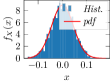
(a)

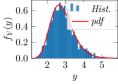
(b)

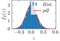
(c)

Figure 2: Histogram and pdf of $2500$ random samples generated from: (a) normal, (b) log-normal, and (c) NLN mixture, with $\mu_{n}=\mu_{nln}=0,\mu_{ln}=1.023$, $\sigma^{2}_{n}=0.002,\sigma^{2}_{ln}=0.048,$ and $\sigma^{2}_{nln}=0.017$.

III-B Normal Log-normal (NLN) Mixture

Broadly speaking, if $X$ and $Y$ are two independent random variables, described by probability density functions $f_{X}(x)$ and $f_{Y}(y)$, then the probability density function of the product $Z=XY$ is given by

$$f_{Z}(z)=\int^{\infty}_{-\infty}f_{X}(x)f_{Y}(z/x)\frac{1}{|x|}\,dx.$$ (7)

More specifically, suppose that $X\sim\mathcal{N}(\mu_{n},\sigma_{n}^{2})$ and $Y\sim\mathcal{LN}(\mu_{ln},\sigma_{ln}^{2})$. Then, the random variable $Z=XY\sim\mathcal{NLN}(\mu_{nln},\sigma_{nln}^{2})$ can be labelled as normal log-normal (NLN) mixture, where its mean $\mu_{nln}$ and variance $\sigma_{nln}^{2}$ are given by [19]

$$\mu_{nln} =\mathbb{E}(XY)=\mathbb{E}(X)\mathbb{E}(Y)=\mu_{n}e^{(\mu_{ln}+0.5\sigma_{ln}^{2})},$$ (8)

$$\sigma_{nln}^{2} =\operatorname{Var}(XY)=\mathbb{E}(X^{2})\mathbb{E}(Y^{2})-(\mathbb{E}XY)^{2},$$

$$=\left(\mu_{n}^{2}+\sigma_{n}^{2}\right)e^{(2\mu_{ln}+2\sigma_{ln}^{2})}-\mu_{n}^{2}e^{(2\mu_{ln}+\sigma_{ln}^{2})}.$$

Let us consider the case where $\mu_{n}=0$, i.e., $X\sim\mathcal{N}(0,\sigma_{n}^{2})$, which is commonly used in sampling-based MPC strategies. Thus, the pdf of $Z$, given in (7), is defined as

$$f_{Z}\!=\!\frac{1}{2\pi\sigma_{n}\sigma_{ln}}\!\!\int_{0}^{\infty}\!\!\!\!\!\exp\!\left(\!-\frac{z^{2}}{2\sigma_{n}^{2}x^{2}}-\frac{(\ln x-\mu_{ln})^{2}}{2\sigma_{ln}^{2}}\!\right)\!\frac{1}{x^{2}}dx,$$ (9)

which can be solved analytically [20]. It is noteworthy that $f_{Z}(z)=f_{Z}(-z)$, indicating a symmetric distribution around $0$ as shown in Fig. 2(c). In addition, $Z$ can be written as a smooth function of two independent normal distributions, i.e., $Z=XY=Xe^{W}$, where $W\sim\mathcal{N}(\mu_{ln},\sigma^{2}_{ln})$. When $\sigma_{n}$ becomes smaller, $X$ places the mass around $0$. This makes the tail of $Z$ lighter than the lognormal distribution. Fig. 2 illustrates different distributions with differing parameters.

III-C log-MPPI Control Strategy

We develop our method on top of the MPPI in [8] for integrating the NLN mixture sampling. Although the original derivation of MPPI is based on the controlled dynamics driven by Brownian motion noise, it can be approximately applied to the NLN mixture, particularly for small $\sigma_{n}$. We provide a discussion on the effect of NLN mixture noise on the dynamics in Appendix A. The major difference is that the trajectories, drawn from the discrete-time dynamics system $\mathbf{x}_{k+1}$, are sampled from the NLN policy, rather than from the Gaussian policy. Accordingly, the control input updates $\delta\mathbf{u}_{k}$ is defined as $\delta\mathbf{u}_{k}=\delta\mathbf{u}^{n}_{k}\cdot\delta\mathbf{u}^{ln}_{k}\sim\mathcal{NLN}(\mathbf{0},\Sigma_{\mathbf{u}})$, where $\delta\mathbf{u}^{n}_{k}\sim\mathcal{N}(\mathbf{0},\Sigma_{n})$, $\delta\mathbf{u}^{ln}_{k}\sim\mathcal{LN}(\mu_{ln},\Sigma_{ln})$, $\Sigma_{\mathbf{u}}=\sigma^{2}_{nln}\mathbf{I}_{m}$, $\Sigma_{n}=\sigma^{2}_{n}\mathbf{I}_{m}$, $\Sigma_{ln}=\sigma^{2}_{ln}\mathbf{I}_{m}$, and $\mathbf{I}_{m}$ denotes an $m\times m$ identity matrix. To ensure that $\delta\mathbf{u}^{ln}_{k}$ is stochastically independent from $\delta\mathbf{u}^{n}_{k}$, Eq. (6) is employed in order to compute $\mu_{ln}$ and $\Sigma_{ln}$, considering $\mu=0$ and $\sigma^{2}=\sigma_{n}$ (namely, standard deviation of $\delta\mathbf{u}^{n}_{k}$). Similarly, Eq. (8) is utilized for computing $\mu_{nln}$ and $\sigma^{2}_{nln}$, taking into account that $\mu_{nln}=0$ as $\mu_{n}=0$.

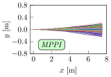
(a)

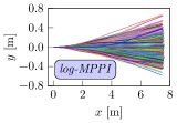
(b)

Figure 3: Distribution of $2500$ sampled trajectories generated by (a) MPPI with $\delta\mathbf{u}_{k}\sim\mathcal{N}(\mathbf{0},0.002\mathbf{I}_{2})$ and (b) log-MPPI with $\delta\mathbf{u}_{k}\sim\mathcal{NLN}(\mathbf{0},0.017\mathbf{I}_{2})$, where the robot is assumed to be located at $\mathbf{x}=[{x},{y},\theta]^{T}=[0,0,0]^{T}$ in ([$\mathrm{m}$], [$\mathrm{m}$], [$\deg$]) with a commanded control input $\mathbf{u}=[v,\omega]^{T}=[1.5,0]^{T}$ in ([$\mathrm{m}\mathrm{/}\mathrm{s}$], [$\mathrm{rad}\mathrm{/}\mathrm{s}$]).

To demonstrate the advantages of sampling from the NLN distribution on the performance of the MPPI algorithm, here we provide a concrete example. The basic idea is to use a small variance (so that we can avoid violating system constraints); yet, we can still get desirable sampled trajectories that are well spread-out for covering large state-space. Specifically, (i) we first draw random samples, namely, $X\equiv\delta\mathbf{u}^{n}_{k}$, from a normal distribution with $\mu_{n}=0$ and $\sigma^{2}_{n}=0.002$ (see Fig. 2(a)); (ii) then, another set of random samples, namely, $Y\equiv\delta\mathbf{u}^{ln}_{k}$, are generated from the corresponding log-normal distribution with $\mu_{ln}=1.023$ and $\sigma^{2}_{ln}=0.048$, as illustrated in Fig. 2(b); (iii) finally, the random variable $Z\equiv\delta\mathbf{u}_{k}$ that represents the product of those two independent variables is generated from the NLN distribution with $\mu_{nln}=0$ and $\sigma^{2}_{nln}=0.017$. Now, let us draw $M$ sampled trajectories from $\delta\mathbf{u}_{k}\sim\mathcal{N}(\mathbf{0},0.002\mathbf{I}_{2})$, as depicted in Fig. 3(a), considering the discrete-time kinematics model of the robot given in (11) and control schemes parameters listed in Section IV-B1, where $M=2500$. In a similar way, Fig. 3(b) shows the sampled trajectories from $\delta\mathbf{u}_{k}\sim\mathcal{NLN}(\mathbf{0},0.017\mathbf{I}_{2})$. It is interesting to observe in Fig. 3 that the distributions of the sampled trajectories generated by the log-MPPI algorithm are more flexible and efficient than the ones generated by the classical MPPI, resulting in (i) better exploration of the state-space, and (ii) reducing the probability of getting trapped in local minima.

One might argue that injecting the same control variance to the normal distribution can lead to similar results. Here, we provide the advantages of the NLN distribution through (i) an analysis from the dynamics perspective in Appendix A where we show that even with the same variance, the proposed scheme can be more efficient due to the random drift term in dynamics, and (ii) the extensive simulation results carried out in the next section which show a much better exploration with more than 30% reduction in the injected noise variance $\Sigma_{\mathbf{u}}$.

IV Simulation-Based Evaluation

We evaluated and compared the two control strategies on a simulated cartpole system and a goal-oriented AGV autonomous navigation task in 2D cluttered environments.

IV-A Cartpole Swing-up Task

To demonstrate the impact of drawing trajectories from the NLN distribution policy, instead of Gaussian policy, on the behavior of the sampling-based MPC algorithm and assess the practical stability of our proposed control strategy, especially with a significantly fewer number of trajectories, we applied MPPI and log-MPPI on a simulated cartpole system.

1)  Simulation Setup:

The main objective is to swing up and stabilize the cartpole for $12\text{\,}\mathrm{s}$. The cartpole dynamics model are taken from [8] with assigning the same values to the system variables, while the pole length $l$ is set to $1\text{\,}\mathrm{m}$ and the instantaneous running cost function is formulated as:

$$q(\mathbf{x})=$10$x^{2}+\numprint{e3}(1+\cos(\theta))^{2}+2\dot{\theta}^{2}+2\dot{x}^{2},$$ (10)

where $x$ and $\dot{x}$ are the horizontal position and velocity of the cart, while $\theta$ and $\dot{\theta}$ denote the angle and angular velocity of the pole. For both control schemes, the simulations were performed with a time prediction $t_{p}$ of $2\text{\,}\mathrm{s}$, a control frequency of $50\text{\,}\mathrm{Hz}$ (sequentially, $N=100$), a $1000$ sampled rollouts at each time-step $\Delta t$, an exploration variance $\nu$ of $1000$, an inverse temperature $\lambda$ of $0.07$, and a control weighting matrix $R$ of $\frac{\lambda}{2}\Sigma_{n}^{-\frac{1}{2}}$ with $\Sigma_{n}=0.0225$ for log-MPPI. The Savitzky-Galoy (SG) convolutional filter, which is utilized for smoothing the control sequence $\left\{\mathbf{u}_{k}\right\}_{k=0}^{N-1}$ computed by Eq. (4), is applied with a quintic polynomial function, i.e., $n_{sg}=5$, and a window length $l_{sg}$ of $51$.

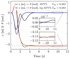
(a)

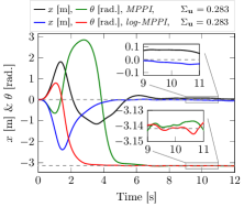
(b)

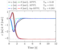
(c)

Figure 4: Performance comparison of MPPI and log-MPPI for the cart–pole swingup task, considering: (a) the same sampling variance, namely, $\Sigma_{\mathbf{u}}=0.283$, while $M=1000$, (b) the same sampling variance, i.e., $\Sigma_{\mathbf{u}}=0.283$, while $M=5$, (c) higher variances in the case of MPPI.

2)  Simulation Results:

We tested the robustness of our proposed algorithm by changing the noise variance $\Sigma_{\mathbf{u}}$, and number of sampled trajectories $M$, as illustrated in Fig. 4. In Figs. 4(a) and 4(b), the simulations are carried out considering two different values of $M$ (namely, $M=1000$ and $5$), while keeping the injected noise variance the same, namely, $\Sigma_{\mathbf{u}}=0.283$. We can notice from Fig. 4(a) that our control scheme achieves a slightly faster convergence; the cartpole converges to the desired configuration (i.e., $x=$0\text{\,}\mathrm{m}$$ and $\theta=\pi\,$\mathrm{rad}$$) within $3.9\text{\,}\mathrm{s}$ compared to $4.8\text{\,}\mathrm{s}$ when MPPI is used. Figure 4(b) demonstrates that the impact of decreasing $M$ on the behavior of MPPI is appreciably higher than its impact on log-MPPI, as the former produced control input that ultimately leads to a higher transient overshoot of $\theta$ and higher positioning error (about $7.6\text{\,}\mathrm{cm}$). On the other side, log-MPPI still performs well with a very slightly positioning error, without compromising its robustness level and convergence rate, which opens up a new avenue for sampling-based MPC algorithm to be run on a standard CPU instead of a GPU, with a fewer number of samples. Furthermore, it is noteworthy that MPPI can achieve similar or better performance of log-MPPI by increasing $\Sigma_{\mathbf{u}}$ at least 73%, as depicted in Fig. 4(c). However, assigning higher values might result in violating the system constraints if they are applied and added to the optimization control problem of the MPPI algorithm.

IV-B Autonomous Navigation in Cluttered Environments

With the aim of demonstrating the prospective advantages of our proposed log-MPPI control strategy compared to the classical MPPI, extensive simulations are conducted in goal-oriented AGV autonomous navigation tasks in 2D cluttered environments.

1)  Simulation Setup:

In this work, we consider the kinematics model of a differential wheeled robot. The kinematics equations that govern the motion of the robot is expressed as

$$\left[\begin{array}[]{c}\dot{x}\\ \dot{y}\\ \dot{\theta}\end{array}\right]=\left[\begin{array}[]{cc}\cos\theta&0\\ \sin\theta&0\\ 0&1\end{array}\right]\left[\begin{array}[]{c}v\\ \omega\end{array}\right]\Leftrightarrow\dot{\mathbf{x}}=\mathcal{R}(\theta)\mathbf{u},\vspace*{-2pt}$$ (11)

where $\mathbf{x}=[{x},{y},\theta]^{T}\in\mathbb{R}^{3}$ represents the pose of the robot expressed in the world frame, $\theta$ is the rotation (or, heading) angle, the control $\mathbf{u}=[v,\omega]^{T}\in\mathbb{R}^{2}$ denote the linear and angular velocities of the robot.

The parameters of both control strategies were set as follows: $t_{p}=$5\text{\,}\mathrm{s}$$ (i.e., $N=250$), $M=2500$, $\nu=1200$, and $R=\lambda\Sigma_{n}^{-\frac{1}{2}}$. However, for MPPI, the inverse temperature $\lambda$ and the control noise variance $\Sigma_{\mathbf{u}}=\operatorname{Diag}\left(\sigma_{v}^{2},\sigma_{w}^{2}\right)$ (herein, $\Sigma_{\mathbf{u}}\equiv\Sigma_{n}$) are set to $0.572$ and $\operatorname{Diag}\left(0.023,0.028\right)$, respectively, while in the case of log-MPPI they are set to much lower values, namely, $0.169$ and $\operatorname{Diag}\left(0.017,0.019\right)$, respectively. In fact, those two hyperparameters were chosen based on the intensive simulations carried out in Tests #1 and #2 in Table I. It can be noticed that $\Sigma_{\mathbf{u}}$, in the case of log-MPPI, is basically computed from a normal distribution with a variance of $\Sigma_{n}=\operatorname{Diag}\left(0.002,0.0022\right)$. For the SG filter parameters, we set $n_{sg}$ and $l_{sg}$ to $3$ and $51$, respectively. The real-time execution of MPPI and log-MPPI is carried out on an NVIDIA GeForce GTX 1660 Ti laptop GPU, where all algorithms were written in Python and were implemented on a differential wheeled robot, namely, ClearPath Jackal robot, integrated with the Robot Operating System (ROS) framework.

Within this work, trajectories are sampled on a GPU using the discrete-time kinematics model given in Eq. (11), where the state-dependent cost function of the 2D navigation task is simply formulated as

$$q(\mathbf{x})=q_{\text{state}}(\mathbf{x})+q_{\text{obs}}(\mathbf{x}),$$ (12)

where $q_{\text{state}}(\mathbf{x})=(\mathbf{x}-\mathbf{x}_{f})^{\mathrm{T}}Q(\mathbf{x}-\mathbf{x}_{f})$ is a quadratic cost function utilized for enforcing the robot current state $\mathbf{x}$ to reach its desired state $\mathbf{x}_{f}$, and $Q=\operatorname{Diag}(5,5,2)\;\forall v_{\text{des}}\leq$1\text{\,}\mathrm{m}\mathrm{/}\mathrm{s}$$, otherwise $Q=\operatorname{Diag}(2.5,2.5,2)$. $q_{\text{obs}}(\mathbf{x})=10^{7}C_{\text{crash}}$ heavily penalizes trajectories that collide with obstacles, where $C_{\text{crash}}$ is a Boolean variable that indicates the collision with obstacles.

2)  Simulation Scenarios:

We considered four various scenarios for evaluating the performance of the proposed control framework in cluttered environments. In Scenario #1, the intensive simulations (namely, $\mathcal{N}_{T}=100$ tasks) are carried out by taking into account different values of $\lambda$ and $\Sigma_{\mathbf{u}}$, with the aim of (i) choosing the best sets of hyperparameters that respect the control constraints, then (ii) assessing the performance in the following scenarios. We choose $\lambda\in[0.01,10]$ and $\Sigma_{\mathbf{u}}\in[0.0004,0.16]$, while a cluttered environment, with obstacles placed $2\text{\,}\mathrm{m}$ away, has been used for assessing the performance. In the last three scenarios, we randomly generated three different types of forests, each type has $50$ forests, i.e., $\mathcal{N}_{T}=50$ tasks, and each forest represents a $$50\text{\,}\mathrm{m}$\times$50\text{\,}\mathrm{m}$$ cluttered environment. In the first type (i.e., Scenario #2), the obstacles were, on average, $1.5\text{\,}\mathrm{m}$ apart (namely, $d^{\text{obs}}_{\min}=$1.5\text{\,}\mathrm{m}$$), whilst in the second (Scenario #3) and third (Scenario #4), they placed $2\text{\,}\mathrm{m}$ and $3\text{\,}\mathrm{m}$ away, respectively. For the first three scenarios, the maximum desired velocity $v_{\text{des}}$ of the robot is set to $1.5\text{\,}\mathrm{m}\mathrm{/}\mathrm{s}$, while in the latter it is allowed for the robot to navigate with its maximum velocity which is $2\text{\,}\mathrm{m}\mathrm{/}\mathrm{s}$.

3)  Performance Metrics:

To achieve a fair performance comparison of the two control schemes: (i) first, in all simulations, the robot has to reach the same desired pose, namely, $\mathbf{x}_{f}=[50,50,0]^{T}$, from the predefined initial pose $\mathbf{x}_{0}=[0,0,0]^{T}$ (in [$\mathrm{m}$], [$\mathrm{m}$], [$\deg$]); (ii) second, we define a set of metrics so as to assess the overall performance such as the number of successful tasks $\mathcal{S}_{T}$, success rate $\mathcal{S}_{R}$, average robot trajectory length $l_{\text{av}}$ to reach $\mathbf{x}_{f}$ from $\mathbf{x}_{0}$, number of successful tasks with a shorter route (i.e., robot trajectory) towards the goal $\mathcal{N}_{l_{\text{min}}}$, and average traveling speed $v_{\text{av}}$. The task is considered to be successful if the robot successfully reaches the desired goal without colliding with obstacles. Note that $l_{\text{av}}$, $\mathcal{N}_{l_{\text{min}}}$, and $v_{\text{av}}$ are only computed for successful tasks $\mathcal{S}_{T}$ that are successfully completed by both control schemes.

TABLE I: Overall performance of the two control schemes, where the gray cells represent better results.

Test	Scheme	$\mathcal{N}_{T}$	$\mathcal{S}_{T}$	$\mathcal{S}_{R}$ [%]	$l_{\text{av}}$ [$\mathrm{m}$] ($\mathcal{N}_{l_{\text{min}}}$)	$v_{\text{av}}$ [$\mathrm{m}\mathrm{/}\mathrm{s}$]
Scenario #1: $v_{\text{des}}=$1.5\text{\,}\mathrm{m}\mathrm{/}\mathrm{s}$$ & $d^{\text{obs}}_{\min}=$2\text{\,}\mathrm{m}$$
#1	MPPI	100	48	48	$-$	$-$
#2	log-MPPI	100	61	61	$-$	$-$
#$\overline{1}$	MPPI	60	21	35	$-$	$-$
#$\overline{2}$	log-MPPI	60	43	71.7	$-$	$-$
Scenario #2: $v_{\text{des}}=$1.5\text{\,}\mathrm{m}\mathrm{/}\mathrm{s}$$ & $d^{\text{obs}}_{\min}=$1.5\text{\,}\mathrm{m}$$
#3	MPPI	50	42	84	76.52 (9/40)	$1.27\pm 0.18$
#4	log-MPPI	50	48	96	75.19 (31/40)	$1.34\pm 0.12$
Scenario #3: $v_{\text{des}}=$1.5\text{\,}\mathrm{m}\mathrm{/}\mathrm{s}$$ & $d^{\text{obs}}_{\min}=$2\text{\,}\mathrm{m}$$
#5	MPPI	50	46	92%	76.19 (13/46)	$1.32\pm 0.14$
#6	log-MPPI	50	50	100	75.29 (33/46)	$1.33\pm 0.11$
Scenario #4: $v_{\text{des}}=$2\text{\,}\mathrm{m}\mathrm{/}\mathrm{s}$$ & $d^{\text{obs}}_{\min}=$3\text{\,}\mathrm{m}$$
#7	MPPI	50	50	100	72.17 (21/50)	$1.82\pm 0.039$
#8	log-MPPI	50	50	100	72.09 (29/50)	$1.84\pm 0.037$

4)  Simulation Results:

The general performance of our proposed control schemes are summarized in Table I, considering the four scenarios defined previously and controllers’ parameters given in Section IV-B1. It is worthy to notice in Scenario #1 (i.e., Tests #1 and #2), where different values of $\lambda$ and $\Sigma_{\mathbf{u}}$ are considered, that log-MPPI significantly outperforms MPPI as its success rate $\mathcal{S}_{R}$ is noticeably higher than that in MPPI, especially for the first $60$ tasks (i.e., $\mathcal{N}_{T}=60$) where lower values are assigned to $\Sigma_{\mathbf{u}}$ (see Tests #$\overline{1}$ and #$\overline{2}$). In practice, this clearly indicates that log-MPPI is largely compatible with a wide range of acceptable parameters values, reducing the time taken for fine-tuning those parameters that play an important role in determining the behavior of sampling-based MPC scheme. For Scenario #2 (i.e., Tests #3 and #4), where $d^{\text{obs}}_{\min}=$1.5\text{\,}\mathrm{m}$$, it can be clearly noticed that our method experimentally exhibits better performance not only due to its higher success rate ($\mathcal{S}_{R}=96\%$), but also due to the fact that: (i) $l_{\text{av}}$ is lightly shorter (roughly, $1.33\text{\,}\mathrm{m}$ shorter than that for MPPI), (ii) $\mathcal{N}_{l_{\text{min}}}$ is quite higher (totally, $31$ tasks compared to $9$ for MPPI), and (iii) $v_{\text{av}}$ is slightly better and closer to $v_{\text{des}}$ with a very low standard deviation. Similarly, in the remaining tests with high values of $d^{\text{obs}}_{\min}$, log-MPPI performs well with a high capability of successfully complete all given tasks while avoiding obstacles; thanks to the NLN distribution policy that provides more flexible and efficient trajectories, we ensure a much better exploration of the state-space of the given system with more than 30% reduction in the injected noise variance and reduce the risk of getting stuck in local minima when MPPI is employed.

In Fig. 5, we show an example of the robot trajectories generated by MPPI and log-MPPI in a cluttered environment, where $d^{\text{obs}}_{\min}=$2\text{\,}\mathrm{m}$$, i.e., Scenario #3. We can clearly observe that although both control schemes achieve successfully collision-free navigation through the cluttered environment with an average traveling speed $v_{\text{av}}$ of $1.33\text{\,}\mathrm{m}\mathrm{/}\mathrm{s}$ which respects the control constraints as the robot linear velocity $v\leq v_{\text{des}}=$1.5\text{\,}\mathrm{m}\mathrm{/}\mathrm{s}$$ as shown in Figs. 5(b) and 5(c), log-MPPI provides a shorter route towards the goal as shown in Fig. 5(a). More precisely, the length of the robot trajectory $l$ in the case of log-MPPI is $77.8\text{\,}\mathrm{m}$ compared to $79.92\text{\,}\mathrm{m}$ for the classical MPPI.

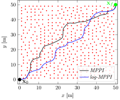
(a) Robot trajectories generated by MPPI and
log-MPPI; red dots represent random obstacles

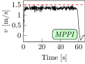
(b) Linear velocity (MPPI)

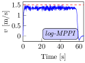
(c) Linear velocity (log-MPPI)

Figure 5: Behavior of MPPI and log-MPPI in a $$50\text{\,}\mathrm{m}$\times$50\text{\,}\mathrm{m}$$ cluttered environment, where obstacles were $2\text{\,}\mathrm{m}$ apart.

IV-C Autonomous Navigation in Unknown Environments

In Section IV-B, where autonomous navigation in cluttered environments is performed, it is assumed that the costmap that represents the environment is priorly known, limiting the applicability of the control schemes as unknown or partially observed environments are the most dominant in robotics applications [1]. To this end, a 2D costmap created by the costmap_2d ROS package is utilized for storing information about the robot’s surrounding obstacles [21] (see Fig. 6(b)). It employs the sensor data acquired from the environment to build a 2D or 3D occupancy grid of the data, where each cell of the occupancy is typically expressed as occupied, free, or unknown; in our case, a 2D occupancy grid map is sufficient for 2D robot navigation. Thereafter, this occupancy grid is utilized as a local costmap to be fed directly into the sampling-based MPC algorithm, for achieving collision-free navigation in either static or dynamic unknown environments.

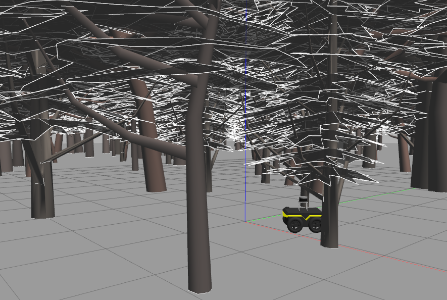
(a)

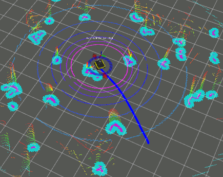
(b)

​​

Figure 6: Snapshot of (a) our Jackal robot located in a forest-like environment, and (b) the corresponding 2D local costmap.

1)  Simulation Setup:

We considered the same simulation setup previously described in Section IV-B1, where the collision indicator function $q_{\text{obs}}(\mathbf{x})$, given in (12), is herein computed based on the local costmap (i.e., 2D grid map) built by the robot on-board sensor; in this work, the Clearpath Jackal robot is endowed with a Velodyne VLP-16 LiDAR sensor. The size of the robot-centered 2D grid map is set to $$240\text{\,}\mathrm{cell}$\times$240\text{\,}\mathrm{cell}$$ with a resolution (grid size) of $0.05\text{\,}\mathrm{m}\mathrm{/}\mathrm{cell}$.

2)  Simulation Scenarios:

For the benchmark, two types of $$50\text{\,}\mathrm{m}$\times$50\text{\,}\mathrm{m}$$ forest-like maps in Gazebo environment are utilized, as depicted in Fig. 6(a). The first type (namely, Forest #1) contains tree shaped obstacles with a density of $0.1\text{\,}\mathrm{trees}\mathrm{/}\mathrm{{}^{2}}\mathrm{m}$, while the latter (i.e., Forest #2) with a density of $0.2\text{\,}\mathrm{trees}\mathrm{/}\mathrm{{}^{2}}\mathrm{m}$. In the case of Forest #1, $v_{\text{des}}$ is set to $2\text{\,}\mathrm{m}\mathrm{/}\mathrm{s}$, while it is reduced to $1.5\text{\,}\mathrm{m}\mathrm{/}\mathrm{s}$ in the case of Forest #2. Another scenario (namely, Corridor #1) is considered in which the robot navigates along a $$6\text{\,}\mathrm{m}$\times$20\text{\,}\mathrm{m}$$ corridor, with $v_{\text{des}}=$1.5\text{\,}\mathrm{m}\mathrm{/}\mathrm{s}$$, in the presence of $8$ pedestrians, each pedestrian holding a maximum velocity of $v_{\text{ref}}=$0.3\text{\,}\mathrm{m}\mathrm{/}\mathrm{s}$$.

3)  Performance Metrics:

Here, we conduct a comparison between the two control schemes in the aspect of the number of collisions $N_{\text{crash}}$, average trajectory length $l_{\text{av}}$, average execution time per iteration $t_{\text{mppi}}$ of the control algorithm. The desired poses (in ([$\mathrm{m}$], [$\mathrm{m}$], [$\deg$])) are defined as follows: $G_{1}=[0,0,0]^{T},G_{2}=[20,20,45]^{T},G_{3}=[-18,2,0]^{T},G_{4}=[20,-21,90]^{T}$, then $G_{5}=[20,20,0]^{T}$. For the sake of simplicity, for Forest #2, the robot navigates autonomously from $G_{1}$ to only $G_{3}$, then stops.

4)  Simulation Results:

Table II summarizes the performance statistics of the two proposed control strategies in Forest #1 and Forest #2, considering 10 trials for each. As anticipated, the obtained results demonstrate that log-MPPI has a more flexible and efficient trajectories sampling distribution policy, resulting in (i) reducing the probability of getting stuck in a local minima (e.g., in Forest #2, $N_{\text{crash}}=1$ compared to $N_{\text{crash}}=7$ when MPPI is used), and (ii) improving the quality of the generated trajectory as $l_{\text{av}}$ is appreciably shorter, especially in Forest #2. Furthermore, we can emphasize that both control schemes guarantee a real-time performance (as $t_{\text{mppi}}<$20\text{\,}\mathrm{ms}$$), showing the superiority of the sampling-based MPC algorithm to be deployed with 2D grid maps without adding any additional complexity to the optimization problem.

For a 2D grid-based navigation in the dynamic environment (namely, Corridor #1), the simulation results demonstrate that the autonomous vehicle successfully avoids moving agents, as shown in the supplementary video. However, we empirically noticed that the more the deployed agents, the noisier the 2D costmap, increasing the risk of being trapped in local minima.

TABLE II: Performance comparisons of MPPI and log-MPPI.

	Forest #1		Forest #2
Indicator	MPPI	log-MPPI	MPPI	log-MPPI
$N_{\text{crash}}$	2	0	7	1
$l_{\text{av}}$ [$\mathrm{m}$]	$158.71\pm 1.54$	$157.91\pm 0.54$	$76.12\pm 3.31$	$72.64\pm 0.80$
$t_{\text{mppi}}$ [$\mathrm{ms}$]	$13.72\pm 1.34$	$13.98\pm 0.68$	$13.70\pm 4.26$	$13.47\pm 1.46$

V Real-World Demonstration

We experimentally demonstrate the applicability of the proposed control strategies for achieving a 2D grid-based collision-free navigation in an unknown indoor cluttered environment.

1)  Experimental Setup:

The simulation setup formerly described in Sections IV-B1 and IV-C1 is also employed for the experimental validation. However, as the indoor environment size is tiny compared to that used for the simulation scenarios, we set $v_{\text{des}}=$0.75\text{\,}\mathrm{m}\mathrm{/}\mathrm{s}$$ and $t_{p}=$8\text{\,}\mathrm{s}$$, while the 2D grid map size is decreased to half of its nominal value (i.e., $$120\text{\,}\mathrm{cell}$\times$120\text{\,}\mathrm{cell}$$) to ensure a real-time implementation of the control strategies. Our experimental platform is a fully autonomous Clearpath Jackal robot equipped with a 16-beam Velodyne LiDAR sensor utilized for (i) generating the local costmap, and (ii) estimating the robot’s pose using LOAM [22].

2)  Validation Environment:

A $$7\text{\,}\mathrm{m}$\times$5.5\text{\,}\mathrm{m}$$ indoor cluttered environment with random boxes as obstacles is utilized for experimental validation, as depicted in Fig. 1(a), where obstacles were, on average, $1.3\text{\,}\mathrm{m}$ apart. Herein, the desired poses (in ([$\mathrm{m}$], [$\mathrm{m}$], [$\deg$])) are given as follows: $G_{1}=[0,0,0]^{T},{{\color[rgb]{0,0,0}G_{2}=[7,5.1,45]^{T}}},G_{3}=[5.5,1.5,0]^{T},G_{4}=[0,3,45]^{T}$, $G_{2}$, then $G_{1}$ (see Fig. 1(a)).

3)  Experimental Results:

The performance statistics for three trials in our indoor environment is summarized in Table III. We can clearly observe, for all trials, that both control schemes provide real-time collision-free navigation, since $N_{\text{crash}}=0$ and $t_{\text{mppi}}<$20\text{\,}\mathrm{ms}$$, in the cluttered environment with an average traveling speed $v_{\text{av}}$ of $0.56\text{\,}\mathrm{m}\mathrm{/}\mathrm{s}$, regardless of the limited perception range. In addition, the quality of the generated trajectories by log-MPPI is considerably better than that generated by MPPI, as $l_{\text{av}}$ is noticeably shorter especially considering the scale of the environment and the density of random obstacles in it. Figure 7 shows a snapshot of the collision-free and predicted optimal trajectories generated by log-MPPI at different time instants while the robot navigates to the desired poses. More details about the experimental results are included in this video: https://youtu.be/bLrQWYLgocw.

TABLE III: Performance statistics of the two control strategies.

Scheme	$N_{\text{crash}}$	$l_{\text{av}}$ [$\mathrm{m}$]	$v_{\text{av}}$ [$\mathrm{m}\mathrm{/}\mathrm{s}$]	$t_{\text{mppi}}$ [$\mathrm{ms}$]
MPPI	0	$40.25\pm 0.13$	$0.55\pm 0.13$	$11.43\pm 0.24$
log-MPPI	0	$38.95\pm 0.17$	$0.57\pm 0.14$	$11.18\pm 0.08$

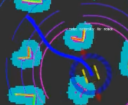
(a)

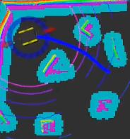
(b)

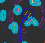
(c)

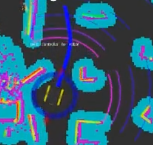
(d)

​​  ​​  ​​

Figure 7: Planned trajectory by log-MPPI using the 2D costmap previously described in Fig. 1(b) (left to right) at $t=$8\text{\,}\mathrm{s}$\,(\!G_{1}\rightarrow G_{2}\!)$, $t=$20\text{\,}\mathrm{s}$\,(\!G_{2}\rightarrow G_{3}\!)$, $t=$31\text{\,}\mathrm{s}$\,(\!G_{3}\rightarrow G_{4}\!)$, and $t=$47\text{\,}\mathrm{s}$\,(\!G_{4}\rightarrow G_{2}\!)$.

VI Conclusion and Future Work

In this work, we proposed an extension to the classical MPPI algorithm (namely, log-MPPI) in which the control input updates $\delta\mathbf{u}_{k}$ are sampled from the normal log-normal (NLN) mixture distribution, rather than from Gaussian distribution. We also presented a sampling-based MPC framework for collision-free navigation in either static or dynamic unknown cluttered environments, by directly integrating the occupancy grid as a local costmap into the sampling-based MPC algorithm. We empirically demonstrated that the trajectory samples generated by log-MPPI are more flexible and efficient than the ones generated by MPPI, with a more than 30% reduction in the injected noise variance $\Sigma_{\mathbf{u}}$ when MPPI is employed. This subsequently results in exploring much better the state-space of the controlled system and reducing the risk of getting stuck in local minima. We demonstrated in real-world environment the possibility of feeding directly the local costmap into the optimal control problem without adding any additional complexity to the control problem, as well as ensuring a real-time performance of the proposed control strategy. In the future, we plan to implement our control scheme on standard CPUs rather than GPUs, aiming to reduce the computational burden. Furthermore, we will explore methods for vanishing the possibility of getting stuck in local minima and studying the theoretical stability of sampling-based MPC.

Appendix A Analysis of the New Sampling Strategy on MPPI

In this appendix, we provide a brief interpretation for the trajectory rollout behavior using the proposed sampling method. Let us examine the effect on the dynamics due to the change of noise. The original dynamics of MPPI reads (i.e., Eq. (53) in [15], ignored constant)

$$\!\!\!\!d\bm{x}_{t}\!=\!\bm{f}(\bm{x}_{t},t)\,dt\!+\!\bm{G}(\bm{x}_{t},t)\bm{u}(\bm{x}_{t},t)\,dt\!+\!\bm{G}(\bm{x}_{t},t)\,d\bm{B}(t),$$ (13)

where $\bm{B}(t)$ is Brownian motion.

In the discrete version, if $\bm{\epsilon}$ in the sampling is replaced by $\bm{Z}=\bm{\epsilon Y}=\bm{\epsilon}e^{\bm{W}}$, where $\bm{W}$ is an independent Gaussian vector of $\bm{\epsilon}$, we may consider this randomness as a new disturbance to the original dynamics. Although it is difficult to obtain an exact dynamics corresponding to the proposed method, we may use the following approximation. Assume that the original $d\bm{B}(t)$ is replaced by $d\left(\bm{B}(t)e^{\mu_{ln}t+\sigma_{ln}\bm{B}_{1}(t)}\right)$, where $\bm{B}_{1}(t)$ is a standard Brownian motion, independent of $\bm{B}(t)$. To simplify notation, denote $\mu_{ln}t+\sigma_{ln}\bm{B}_{1}(t)$ by $\bm{W}_{1}$, and $\kappa\triangleq\frac{1}{2}\sigma_{ln}^{2}+\mu_{ln}$. By Ito’s formula, we can get the following computation for $d\left(\bm{B}(t)e^{\bm{W}_{1}(t)}\right)$:

$$e^{\bm{W}_{1}(t)}d\bm{B}(t)+\bm{B}(t)de^{\bm{W}_{1}(t)}+d[\bm{B}(t),e^{\bm{W}_{1}(t)}]$$

$$=e^{\bm{W}_{1}\!(t)}d\bm{B}(t)\!+\!\!\bm{B}(t)\!\left(\!\sigma_{ln}e^{\bm{W}_{1}\!(t)}d\bm{B}_{1}\!(t)\!+\!\kappa e^{\bm{W}_{1}\!(t)}\!dt\!\right)\!.$$ (14)

Thus, the sampling dynamics can be viewed as a modified one

$$d\bm{x}_{t}=\bm{f}(\bm{x}_{t},t)\,dt+\bm{G}(\bm{x}_{t},t)\bm{u}(\bm{x}_{t},t)\,dt$$

$$+\bm{G}(\bm{x}_{t},t)\,d\left(\bm{B}(t)e^{\bm{W}_{1}(t)}\right)$$

$$=\bm{f}(\bm{x}_{t},t)\,dt+\bm{G}(\bm{x}_{t},t)\left(\bm{u}(\bm{x}_{t},t)+\kappa\bm{B}(t)e^{\bm{W}_{1}(t)}\right)dt$$

$$+\bm{G}(\bm{x}_{t},t)\left(e^{\bm{W}_{1}(t)}d\bm{B}(t)+\sigma_{ln}\bm{B}(t)e^{\bm{W}_{1}(t)}d\bm{B}_{1}(t)\right).$$ (15)

We have two observations. First, the drift term (the term with $dt$) is modified to $\bm{f}(\bm{x},t)+\bm{G}(\bm{x},t)\bm{u}(\bm{x}_{t},t)+\kappa\bm{G}(\bm{x},t)\bm{B}(t)e^{\bm{W}_{1}(t)}$. This can be thought of a random drift term, compared to the deterministic counterpart in the original dynamics. But the mean of the drift term remains the same with the original one. Since the drift term can be viewed as the “trend" of the path for each sample path, the proposed scheme has more diverse “trends" of the trajectories than the original one. The new sampled trajectories turn to spread out much more than that in the original dynamics, indicating that this scheme can explore more spaces than the original one. This leads to a more efficient sampling scheme than the normal distribution, even with the similar variance. Second, the noise term can be much more flexible to tune the variance of the sampling trajectories as it contains more parameters.

References

- [1] I. S. Mohamed, G. Allibert, and P. Martinet, “Model predictive path integral control framework for partially observable navigation: A quadrotor case study,” in 16th Int. Conf. on Control, Automation, Robotics and Vision (ICARCV), Shenzhen, China, Dec. 2020, pp. 196–203.
- [2] D. Q. Mayne, J. B. Rawlings, C. V. Rao, and P. O. Scokaert, “Constrained model predictive control: Stability and optimality,” Automatica, vol. 36, no. 6, pp. 789–814, 2000.
- [3] M. Gaertner, M. Bjelonic, F. Farshidian, and M. Hutter, “Collision-free MPC for legged robots in static and dynamic scenes,” in IEEE Int. Conf. on Robotics and Automation (ICRA), 2021, pp. 8266–8272.
- [4] B. Lindqvist, S. S. Mansouri, A.-a. Agha-mohammadi, and G. Nikolakopoulos, “Nonlinear MPC for collision avoidance and control of UAVs with dynamic obstacles,” IEEE robotics and automation letters, vol. 5, no. 4, pp. 6001–6008, 2020.
- [5] B. Brito, B. Floor, L. Ferranti, and J. Alonso-Mora, “Model predictive contouring control for collision avoidance in unstructured dynamic environments,” IEEE Robotics and Automation Letters, vol. 4, no. 4, pp. 4459–4466, 2019.
- [6] M. A. Abbas, R. Milman, and J. M. Eklund, “Obstacle avoidance in real time with nonlinear model predictive control of autonomous vehicles,” Canadian journal of electrical and computer engineering, vol. 40, no. 1, pp. 12–22, 2017.
- [7] X. Zhang, A. Liniger, and F. Borrelli, “Optimization-based collision avoidance,” IEEE Transactions on Control Systems Technology, vol. 29, no. 3, pp. 972–983, 2020.
- [8] G. Williams, A. Aldrich, and E. A. Theodorou, “Model predictive path integral control: From theory to parallel computation,” Journal of Guidance, Control, and Dynamics, vol. 40, no. 2, pp. 344–357, 2017.
- [9] G. Williams, P. Drews, B. Goldfain, J. M. Rehg, and E. A. Theodorou, “Aggressive driving with model predictive path integral control,” in IEEE Int. Conf. on Robotics and Automation (ICRA), 2016, pp. 1433–1440.
- [10] ——, “Information-theoretic model predictive control: Theory and applications to autonomous driving,” IEEE Transactions on Robotics, vol. 34, no. 6, pp. 1603–1622, 2018.
- [11] H. Lu, Q. Zong, S. Lai, B. Tian, and L. Xie, “Real-time perception-limited motion planning using sampling-based MPC,” IEEE Transactions on Industrial Electronics, 2022.
- [12] I. S. Mohamed, G. Allibert, and P. Martinet, “Sampling-based MPC for constrained vision based control,” in IEEE/RSJ Int. Conf. on Intelligent Robots and Systems (IROS), 2021, pp. 3753–3758.
- [13] M. Bhardwaj, B. Sundaralingam, A. Mousavian, N. D. Ratliff, D. Fox, F. Ramos, and B. Boots, “STORM: an integrated framework for fast joint-space model-predictive control for reactive manipulation,” in Conference on Robot Learning. PMLR, 2022, pp. 750–759.
- [14] I. S. Mohamed, “MPPI-VS: Sampling-based model predictive control strategy for constrained image-based and position-based visual servoing,” arXiv preprint arXiv:2104.04925, 2021.
- [15] G. Williams, B. Goldfain, P. Drews, K. Saigol, J. M. Rehg, and E. A. Theodorou, “Robust sampling based model predictive control with sparse objective information,” in Robotics: Science and Systems, 2018.
- [16] J. Pravitra, K. A. Ackerman, C. Cao, N. Hovakimyan, and E. A. Theodorou, “-adaptive MPPI architecture for robust and agile control of multirotors,” in IEEE/RSJ Int. Conf. on Intelligent Robots and Systems (IROS), 2020, pp. 7661–7666.
- [17] J. Yin, Z. Zhang, E. Theodorou, and P. Tsiotras, “Improving model predictive path integral using covariance steering,” arXiv preprint arXiv:2109.12147, 2021.
- [18] N. L. Johnson, S. Kotz, and N. Balakrishnan, “Lognormal distributions,” in Continuous univariate distributions, volume 2. John wiley & sons, 1995, vol. 289.
- [19] V. K. Rohatgi and A. M. E. Saleh, An introduction to probability and statistics, 3rd ed., D. J. Balding, N. A. Cressie, G. M. Fitzmaurice, G. H. Givens, H. Goldstein, G. Molenberghs, D. W. Scott, A. F. Smith, R. S. Tsay, and S. Weisberg, Eds. John Wiley & Sons, 2015.
- [20] P. K. Clark, “A subordinated stochastic process model with finite variance for speculative prices,” Econometrica: journal of the Econometric Society, pp. 135–155, 1973.
- [21] E. Marder-Eppstein, D. V. Lu!!, and D. Hershberger. Costmap_2d package. [Online]. Available: http://wiki.ros.org/costmap_2d
- [22] J. Zhang and S. Singh, “LOAM: Lidar odometry and mapping in real-time.” in Robotics: Science and Systems, vol. 2, no. 9. Berkeley, CA, 2014, pp. 1–9.