On the physical nature of the Wilson-Bappu effect: revising the gravity and temperature dependence

Abstract

We present a sample of 32 stars of spectral types G and K, and luminosity classes I to V, with moderate activity levels, covering four orders of magnitude of surface gravity and a representative range of effective temperature. For each star we obtained high S/N TIGRE-HEROS spectra with a spectral resolving power of $R\approx 20,000$ and have measured the Ca ii K line-widths of interest, $W_{0}$ and $W_{1}$. The main physical parameters are determined by means of iSpec synthesis and Gaia EDR3 parallaxes. Mass estimates are based on matching to evolution models. Using this stellar sample, that is highly uniform in terms of spectral quality and assessment, we derive the best-fit relation between emission line width and gravity $g$, including a notable dependence on effective temperature $T_{\rm eff}$, of the form $W_{1}\propto g^{-0.229}T_{\rm eff}^{+2.41}$. This result confirms the physical interpretation of the Wilson-Bappu effect as a line saturation and photon redistribution effect in the chromospheric Ca ii column density, under the assumption of hydrostatic equilibrium at the bottom of the chromosphere. While the column density (and so $W_{1}$) increases towards lower gravities, the observed temperature dependence is then understood as a simple ionization effect – in cooler stars, Ca ii densities decrease in favor of Ca i.

1 Introduction

Since Eberhard & Schwarzschild (1913), chromospheric emission in the Ca ii H&K doublet lines ($\lambda_{\text{H}}$ = 3968.47 Å and $\lambda_{\text{K}}$ = 3933.68 Å) is understood to be a universal phenomenon, connected with stellar magnetic activity, and shared by very different kind of late-type stars, which reaches over a wide range of gravities, from Sun to red giants and supergiant stars.

Much of what we know today about chromospheric emission is based on the pioneering work of Olin C. Wilson and his group at the Mount Wilson Observatory, spanning 6 decades of his life. Obviously, strength and width of that emission contains vital information of the chromospheric heating processes and fundamental physical properties of this otherwise elusive atmospheric layer.

One of the most recognized publications of O. C. Wilson’s scientific legacy is his work with M. K. Vainu Bappu of 1957 (Wilson & Bappu, 1957), in which an empirical and apparently universal relation was found between the line width $\log W_{0}$ of the Ca ii K chromospheric emission, taken at half-peak intensity, and the stellar absolute visual magnitudes for a sample of 185 late-type stars. Hampered by the lack of precise distances, Wilson (1967) tried to improve this empirical relation. The same lack of precision in giant luminosities, whose parallaxes were too small to be measured directly in those days, made it impossible to test for the dependence on effective temperature and other physical parameters, and to this day it also remains debated, how precise and universal that relation is.

A major factor in the formation of the observed chromospheric emission line profile is the numerous photon absorption and re-emission processes occurring between the bottom of chromosphere, where the emission is produced, and the top, where the observed line profile emerges. In the absence of considerable collision rates for the Ca ii H&K transition because of the low chromospheric densities, almost always an absorbed photon is re-emitted. As laid out by Ayres et al. (1975), during this process the photons migrate towards the wings of the line profile function, where their escape probability is greater, since the optical depth there is less.

Consequently, there is a line broadening effect, caused by the large optical depth and saturation at the centers of the Ca ii H&K lines, which depends on the column density present in each particular chromosphere. This widening effect is larger for stars with lower gravity, notably giant stars. More luminous giants have a lower gravity, for which hydrostatic equilibrium at the bottom of the chromosphere demands larger scale heights and consequently, a broader Ca ii H&K emission.

In particular, the many absorption and re-emission processes that each emerging photon undergoes, is favoring a migration into the wings of the line profile function, which results (as briefly explained above) in the density broadening of the emission line. The simple explanation of this process by Ayres et al. (1975) and Ayres (1979) suggests a clear relation between column density $N$ and gravity $g$ ($N\propto 1/\sqrt{g}$) and yields a dependence of the foot-to-foot emission-line width $W_{1}$ with gravity of the order of $W_{0}\propto g^{-0.25}$. Comparing giants with known physical parameters, this is essentially consistent with observations (see, e.g. Ayres et al. (1975), Lutz & Pagel (1982), or Park et al. (2013), to name a small selection of work done on this topic). However, in such work, hitherto a 1:1 relation between the two respective line widths $W_{1}$ and $W_{0}$ has always been implied, simply relying on the idea of homologous emission line profiles.

The other important factor, apart from gravity, in the dependence of emission-line width on physical parameters is the effective temperature $T_{\text{eff}}$, since the ionization balance Ca ii:Ca i matters for the Ca ii column density as well. Underestimating this term can severely reduce the apparent dependence on gravity, since the giants higher up in the RGB and AGB are not only characterized by a lower gravity but also a lower effective temperature. This establishes cross-talk and the necessity to solve very well for the dependence on both these physical stellar parameters. However, the notoriously difficult task to assess $T_{\text{eff}}$ with cool giants has hindered exactly all efforts in this regard.

Another complication arises from the effects of strong activity on the chromospheric emission line width, as found with very active binaries (see Montes et al. (1994)). Apparently, the emission line width can be broaden by local plasma motions along magnetic loops. This adds to the above density broadening in the non-active chromosphere and, when not taken into consideration, can offset efforts to find the correct relation of the pure density broadening with the fundamental physical parameters. In this context, it is important to recognize that chromospheric emission increases, by virtue of rising magnetic activity, on the upper AGB (Schröder et al., 2018). On the other hand, to obtain a precise width measurement, it is desirable to have an emission that exceeds the basal flux. Hence, moderate activity seems acceptable in a suitable stellar sample, but strong activity must be avoided.

This study attempts to be conscious of the above described problems and is an attempt to improve the empirical basis for the physical relation behind the Wilson-Bappu effect. Our motivation is to verify the interpretation of Ayres et al. (1975) as a density broadening effect to a higher level of confidence than previous studies. The alternative suggestion of a Doppler broadening by turbulence (e.g. Reimers (1973), and see extensive discussion in Lutz & Pagel (1982)), seems unlikely already because the inferred turbulent velocities would have to become clearly supersonic in giants and supergiants.

In order to deliver a most precise assessment of the physical relation underlying the Wilson-Bappu effect, we here present a sample of cool stars, covering four orders of magnitude of gravity and a representative range of effective temperatures, for which we obtained high S/N (typically 50-70 at Ca ii K), $R\approx 20,000$ TIGRE spectra of a uniform quality across the sample. In addition, we assess the physical parameters uniformly with a consistent method, as described below, using the precise Gaia EDR3 parallaxes to minimize spectroscopic analysis ambiguities and cross talk between poorly derived physical parameters. We developed a method, dealing well with the residual noise on the observed emission line profiles, to measure both line widths of interest ($W_{0}$ and $W_{1}$). Verifying their relation, which is not exactly 1:1, we find this to be an additional, hitherto neglected factor in the comparison of theoretical prediction (using $W_{1}$ with observation based on O.C. Wilson’s $W_{0}$, which can be measured to higher precision).

2 Observations

2.1 The stellar sample

In order to revise, how the widths of the K emission-line of Ca ii behave as a function of (a) the surface gravity $\log g$ and (b) the effective temperature $T_{\text{eff}}$, we selected a sample of 32 well know stars with spectral types G and K, and luminosity classes I to V. This representative selection covers the large range of $\log g$ from 0.9 to 4.5 dex, while $T_{\text{eff}}$ values reach from 3844 to 6013 K (see Table 1). The latter is restricted by the tested reliability of spectroscopic assessment consistency (details are described below).

The state of activity is mostly low to moderate, see the plots of the chromospheric Ca ii K emission line profiles in Appendix B. Apart from the aforementioned complications with the emission from very active regions in the chromosphere, we also avoid another problem: the rotational velocities and their variation across the sample remain within the spectral resolution of TIGRE-HEROS (see below), which is equivalent to 7.5 km/s. Only some of the most active giants reach rotation velocities of over 8 km/s, see e.g. Aurière et al. (2015) (Table 3 therein). The same can be said about the turbulent velocities (of the order of several km/s in both, the photosphere and lower chromosphere), which should – by comparison to the widening by the Wilson Bappu effect – not be of much significance.

Included in our sample are the four Hyades K giants, which mark – according to their X-ray and other activity properties, see Schröder et al. (2020) – low to strong solar activity. The other sample stars fall into this range as well. Please note, that (1) the scales in Appendix B are not the same, (2) the photospheric line depths vary a lot, giving large contrast in a cool giant like Arcturus to even the pure basal chromospheric flux, and (3) even the strongest solar activity, in the wider stellar context, is very moderate by comparison.

Thanks to the recently published parallaxes of the Gaia EDR3 catalogue (Gaia Collaboration et al., 2021) of the ESA Gaia mission (Gaia Collaboration et al., 2016) and using reasonable estimates of the stellar mass $M_{\star}$ from evolution tracks that match the luminosity $L$ and $T_{\text{eff}}$ of each respective star, derived provisionally by a spectral fitting process, we obtained the parallax-based surface gravities, which in turn help to maximize the non-spectroscopic information on each star. In an iterative approach, we then improved the effective temperature derived for each star from spectral synthesizing by selecting for those least residuals solutions, which reproduce the respective calculated gravity.

Only in four cases, with the three very bright stars $\alpha$ Tau (HD 29139), $\alpha$ Hya (HD 81797) and $\alpha$ Boo (HD 124897), as well as the bright eclipsing binary $\zeta$ Aur (HD 32068), Gaia’s EDR3 parallaxes are not reliable. In these cases, we used the Hipparcos parallaxes (ESA, 1997), instead, since their accuracy is not limited so much for the brightest stars, and for $\zeta$ Aur it is in good agreement with the distance obtained from the observed binary system information (see Schröder et al. (1997)).

2.2 Spectroscopic observations with TIGRE

To start with a homogeneous set of spectra of comparable quality, all stars of this sample were observed with the 1.2 m robotic telescope TIGRE (Schmitt et al., 2014) located near Guanajuato, central Mexico. It is equipped with the HEROS echelle spectrograph, which has a moderately-high uniform resolution of $R\approx 20,000$ over the broad wavelength range from about 3800 to 8800 Å, and produces spectra of good quality – typically S/N $\sim$ 100 or more, averaged over the spectrum, which corresponds to 50-70 in the Ca ii H&K line region of a cool star.

The broad wavelength coverage of HEROS is achieved by two separate channels and cameras (for red and blue light, named channel R and channel B). In this way, the cameras and the cross-dispersers are individually optimized for each wavelength region in sensitivity, the echelle orders well separated, and resolution kept uniform. There is only a small gap of about 120 Å around 5800 Å (located on the blue side of the sodium D line), caused by the characteristics of the dichromatic beam splitter.

The advantage of TIGRE-HEROS spectra is the versatility of their use. While we obtain information on the chromospheric Ca ii H&K emission from the B channel spectra, the R channel spectral range is more suitable to spectral synthesizing and the R camera has the best S/N. Flexible scheduling of the robotic telescope provided us with the required observations, including several takes of each star, over the course of about a year.

To improve our measurements of Ca ii K emission-line widths, we typically added two or three spectra of the B channel, following a quality control by eye to discard anomalous differences between different takes. With this approach, we avoided the effects of electronic noise or under-exposure in nights of bad transparency, optimize S/N, as well as our measurements of the emission line widths.

3 Deriving the physical parameters

3.1 Calculation of parallax-based gravities

In a first step to calculate the parallax-based gravities, we derived absolute visual magnitudes via the Gaia EDR3 parallaxes and available photometry, and estimated stellar masses $M_{\star}$ using an approximate preliminary analysis of its position in the Hertzsprung-Russell diagram to find the matching evolution track. We used the photometric apparent magnitudes from the SIMBAD database in the $V$ band ($m_{V}$), as well as the color index $B-V$. The parallaxes in milliarcseconds (and distances in parsecs) were taken from the Gaia EDR3 archive. We applied the parallax zero-point correction of Lindegren et al. (2021), using their published Python code. No interstellar extinction correction was applied, because the average distance of our sample stars is below $\sim 100$ pc.

To determine the bolometric magnitudes and, finally, each luminosity, we applied the bolometric corrections (BC) from Flower (1996) for which the effective temperature $T_{\text{eff}}$, or the color index $B-V$, is required. As a start value (to be refined later) for the $T_{\text{eff}}$ we used the average of the PASTEL catalogue entries (Soubiran et al., 2016) for each sample star.

Flower (1996) expresses the bolometric correction in the $V$-band ($\text{BC}_{V}$) as a function of the effective temperature of the form: $\text{BC}_{V}=a+b(\log T_{\text{eff}})+c(\log T_{\text{eff}})^{2}+...$, for three different temperature ranges. The coefficients $a,b,c,...$ are shown in his Table 6 for each interval, but because of a typographical error, the powers of those coefficients were omitted. A fact that was clarified and corrected by Torres (2010). In addition, Flower (1996) calculates $\log T_{\text{eff}}$ as a function of color index of the form $\log T_{\text{eff}}=a+b(B-V)+c(B-V)^{2}+...$ where the coefficients $a,b,c,...$ are taken separately for supergiants or for main sequence stars, subgiants and giants. However, the values of $\text{BC}_{V}$ differ a bit, depending on whether the color index or the effective temperature is used. To have a better approximation and eliminate possible differences, we used the average of the resulting two values of $\text{BC}_{V}$, derived from $B-V$ and $T_{\text{eff}}$, respectively. Finally, the luminosity in solar units was calculated using the relation $\log L=(4.74-M_{V}-\text{BC}_{V})/2.5$, where we applied a solar visual absolute magnitude of 4.74.

Using the stellar luminosities and effective temperatures, the stars were located in a Hertzsprung-Russell diagram (HRD). The $\text{M}_{\star}$ were estimated using a grid of stellar evolution tracks that we computed with the Cambridge (UK) Eggleton code in its updated version (Pols et al. (1997), Pols et al. (1998)), with the quasi-solar metallicity of $Z=0.02$ (see Fig. 1).

According to the PASTEL catalogue, our sample has an average metallicity of $-0.05$ dex, i.e. close to solar metallicity. However, taking into account the residual differences, we need to consider that any smaller metallicity makes a star of given mass and age more luminous and less cool, caused by its lower opacities, and the stellar position in the HRD is shifted to the lower left, see e.g. Schröder et al. (2013). Consequently, because of such miss-matches based on the residual differences of the stellar metallicites from solar, we considered an uncertainty for each stellar mass estimate of about 10 percent.

Finally, the surface gravity of each sample star was calculated from the respective stellar luminosity, mass, and (initial) effective temperature as follows. If $R_{\star}$ is the stellar radius, $\log L\propto\log(R_{\star}^{2}T_{\text{eff}}^{4})\propto\log(\text{M}_{\star}g^{-1}T_{\text{eff}}^{4})$. Finally, if $\log g_{\odot}=4.437$ (in units of cgs) is the solar surface gravity, the surface gravity is given by

$$\log g=4.437+\log\left(\dfrac{\text{M}_{\star}}{\text{M}_{\sun}}\right)-\log\left(\dfrac{L}{L_{\sun}}\right)+4\log\left(\dfrac{T_{\text{eff}}}{T_{\sun}}\right).$$ (1)

Using equation 1, this resulted in preliminary gravities for the sample. We used this value to derive the effective temperatures by means of spectral synthesizing (see below), avoiding solutions with wrong gravity and the resulting cross-talk into $T_{\text{eff}}$, see (Schröder et al., 2021). Then the calculated gravities were updated with these self-determined $T_{\text{eff}}$ values. We repeated this procedure to finally refine the effective temperatures as well, where needed. Table 2 summarizes our final results for all 32 stars used in this study.

3.2 Deriving effective temperatures by spectral synthesizing

To derive stellar parameters, $T_{\text{eff}}$ in particular from the R channel of TIGRE-HEROS, we used the spectral analysis toolkit iSpec (Blanco-Cuaresma et al., 2014b) in its latest Python 3 version (v2020.10.01) (Blanco-Cuaresma, 2019). It allows a comparison of an observed spectrum with synthetic spectra, interpolated from atmospheric models of different physical parameters. The best match, defined by the least differences ($\chi^{2}$ method) then defines, at least in principle, the corresponding physical parameters. However, in practice there are a number of complications, mostly of physical nature, as pointed out by Schröder et al. (2021). Therefore, information external to the spectroscopic synthesizing is vital to allow testing and to filter seemingly equivalent best-fit solutions.

These problems are mostly caused by a large minimal $\chi^{2}$ level, produced by the residual mismatches of line strengths (atomic $f$-values), as well as by subtle, unnoticed blends with other lines – even in a well-selected, representative subset of seemingly reliable lines. Furthermore, any such subset is only representative and usable for a limited range of effective temperatures. In addition, towards the low end of stellar effective temperatures, NLTE effects may be mismatched by the model libraries that iSpec can use. These complications set limits and require a careful handling of the parameter assessment, applied consistently to all sample stars.

We applied the spectral synthesis process to determine the stellar parameters only in the R-channel of the spectrum, given its better S/N in comparison with the B-channel of HEROS, and its lesser line density, better avoiding line blends interfering with the analysis. We then developed an iSpec script (iSPar v4.4.3), written in Python 3, to perform the spectral synthesizing by an algorithm, which uses the very useful iSpec tools in a consistent manner.

We used the grid of marcs atmosphere models (Gustafsson et al., 2008) included in iSpec. For the reference solar abundances, we used the values published in Grevesse et al. (2007). The synthetic spectra were calculated using the radiative transfer code turbospectrum version 15.1 (Alvarez & Plez (1997), Plez (2012)), which uses already spherical models instead of the plane-parallel approximation (a better approach for giant stars).

When spectral synthesis methods are applied to spectroscopic analysis, parameter determination is complicated by having to fit several of them at the same time, as this approach causes a multitude of ambiguous best-fit solutions. These are caused by the fact that one mismatched parameter can be compensated in its effect by the mismatch of others, named as cross-talk, still resulting in a seemingly good representation of the observed spectrum. iSpec therefore finds different solutions in parameter space, depending on the choice of the initial values, which all need to be explored and tested. We based our algorithm therefore on the considerations of Schröder et al. (2021), who showed a fast method for determining the physical parameters of main sequence stars with moderate resolution spectra, where that was possible. For example, there are no reliable $ubvy$-photometry-derived metallicity values available for giant stars. Still, our script aims on minimizing cross-talk by maximizing the use of non-spectroscopic information to filter out those best-fit solutions with parameters contradicting that information external to the synthesizing process.

A very delicate procedure preceding the synthesizing step is the fit of the pseudo-continuum of the observed stellar spectrum in question and the line selection for the synthesizing procedure with iSpec. After several comparative tests, we found that the impact of this step on the final results of the stellar parameters is not negligible, since it affects the $\chi^{2}$ sums and their minima in parameter space. We explain in detail the pseudo-continuum adjustment and the line selection in the appendix A. The latter is important for the successful spectroscopic synthesizing and is a compromise between completeness and quantity versus line data quality.

3.2.1 Final stellar parameter determination

For the final analysis of the now readjusted, normalized observed spectrum by parameter synthesizing, we set the start values to the averages of $T_{\text{eff}}$ and [M/H] in the PASTEL catalogue, while the initial gravities were calculated using equation 1. Initial $v_{\text{mic}}$ values – as detailed in the appendix A for the synthetic spectra used to guide the continuum readjustment – are set to the velocities used for the phoenix library (Husser et al., 2013), while $v_{\text{mac}}$ is set again by equation 4.

The best-fit results of iSpec synthesizing are sensitive to the choice of the initial parameters. The further exploration of the parameter space therefore follows the strategy of Blanco-Cuaresma et al. (2014b), varying the initial values in steps. Our iSpec script implements an analysis that varies the initial parameters by as much as follows: $\pm 100$ K for $T_{\text{eff}}$, $\pm 0.15$ dex for $\log g$, and $\pm 0.15$ dex for [M/H], each time repeating the process for a total of 27 calculations around the initial values. Then stellar parameters with the best $\chi^{2}$ result of all solutions is chosen. These step-sizes and the following sequence performed best in our tests described in subsection 3.4.

Based on the strategy of Schröder et al. (2021), the best way to determine the stellar parameters is to leave only one of them free at a time, while the others remain fixed, going through the following sequence in a partially iterative procedure: (1) refine $v_{\text{mic}}$; (2) having re-set $v_{\text{mac}}$ through equation 4, based on the now refined $v_{\text{mic}}$, refine gravity ($\log{g}$); (3) now refine $v\sin i$; (4) refine $T_{\text{eff}}$, [M/H] and $\text{[}\alpha\text{/Fe]}$; (5) refine $v_{\text{mac}}$; (6) refine again $v_{\text{mic}}$; (7) refine again $T_{\text{eff}}$, [M/H] and $\text{[}\alpha\text{/Fe]}$; (8) refine again $v\sin i$ and finally, (9) refine again [Fe/H]. However, with the resolution of TIGRE–HEROS spectra in mind, we are aware that different turbulence and rotation velocity values under 3 km/s bear no physical meaning, considering our modest spectral resolution. Still, there is a need to adjust them in a tested way to minimize cross talk (see below). We should also note, for the complications with cross-talk in combination with the limited spectral resolution, that we do not consider the rotation and turbulence velocity values derived here of any credibility because they are typically half the instrumental line profile width. Our tests only demonstrate the reliability of the main physical parameters, namely effective temperature, gravity, and metallicity.

3.3 Consistency check with parallax-based gravities

The improved values of $T_{\text{eff}}$ obtained from spectral synthesis with our iSpec script give slightly different positions in the HR diagram. We therefore repeated, at this point, the mass estimates and, consequently, recalculated the parallax-based gravities (in the same way as in subsection 3.1), and finally also repeated all synthesizing steps of above. Table 1 summarizes the final stellar parameters obtained for the sample stars with this method, while Table 2 details the distances, magnitudes, physical parameters and parallax-based gravities. Fig. 1 pictures the final estimation of the masses for the stellar sample on a grid of stellar evolution tracks, computed with the Cambridge (UK) Eggleton code for solar metallicity.

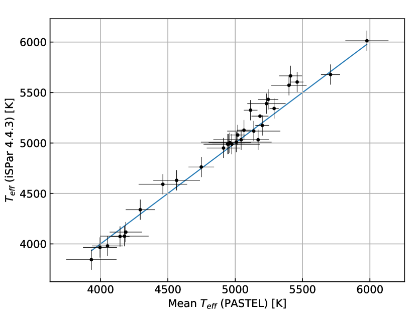
Figure 2: Temperature comparison between the values calculated by spectral synthesis using our iSpec script and the average values in the PASTEL catalogue.

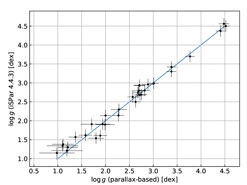
Figure 3: Surface gravity comparison between the values calculated by spectral synthesis using our iSpec script and the parallax-based gravities using the equation 1.

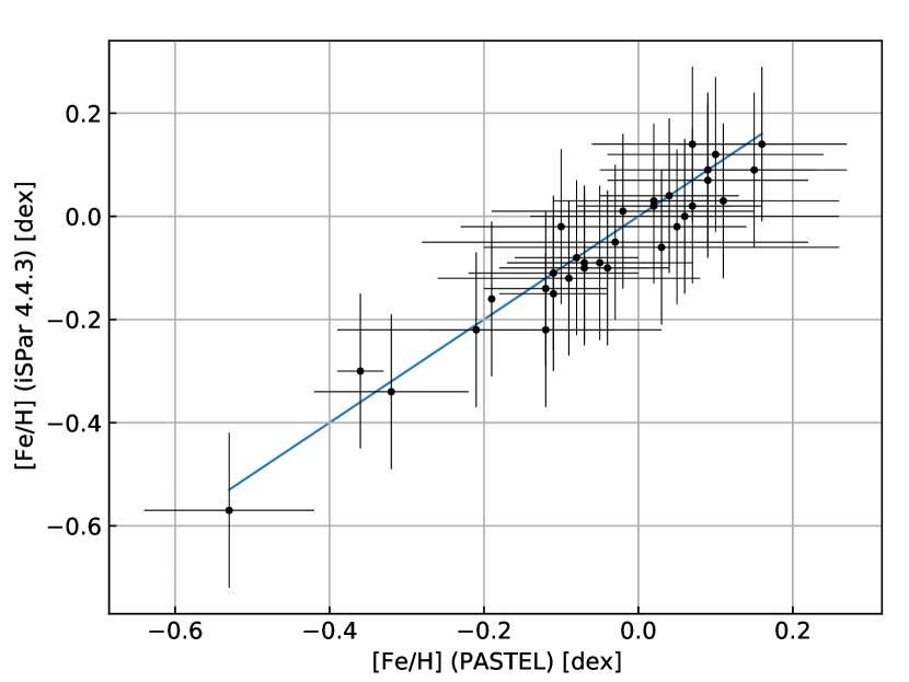
Figure 4: Metallicity comparison between the values calculated by spectral synthesis using our iSpec script and the average values in the PASTEL catalogue.

To ensure that our assessment of the stellar parameters of the sample is sufficiently reliable, we tested our results as follows: Fig. 2 and Fig. 4 show a comparison between our results for $T_{\text{eff}}$ and [Fe/H] by spectral synthesis (as described above) and the average values in the PASTEL catalogue. Fig. 3 shows a comparison between our results for $\log g$ by spectral synthesis and the parallax-based gravities of Table 2. The blue line in these graphs represents the ideal of a 1:1 relation; the uncertainties of our estimations were calculated as explained in subsection 3.4.

Table 1: Stellar parameters derived with our iSpec script.

Star	Typea	$T_{\text{eff}}$b	$\log g$c	[M/H]	$\text{[}\alpha\text{/Fe]}$	$v_{\text{mic}}$d	$v_{\text{mac}}$d	$v\sin{i}$d	[Fe/H]
		[K]	[dex]	[dex]	[dex]	[km/s]	[km/s]	[km/s]	[dex]
HD 8512	K0IIIb	4762 (17)	2.50 (0.04)	-0.15 (0.01)	0.04 (0.02)	1.66	3.44	0.00	-0.15 (0.01)
HD 10476	K1V	5174 (24)	4.50 (0.02)	-0.10 (0.02)	0.01 (0.02)	0.96	0.00	0.00	-0.10 (0.02)
HD 18925	G9III	5032 (26)	2.30 (0.00)	-0.17 (0.02)	-0.04 (0.03)	1.39	3.67	1.20	-0.16 (0.01)
HD 20630	G5V	5678 (43)	4.56 (0.05)	-0.03 (0.04)	0.01 (0.04)	1.31	3.70	0.60	-0.02 (0.02)
HD 23249	K0+IV	5032 (28)	3.70 (0.06)	0.03 (0.02)	0.02 (0.03)	1.18	0.48	0.00	0.00 (0.02)
HD 26630	G0Ib	5572 (31)	1.90 (0.11)	0.01 (0.02)	0.02 (0.03)	3.25	5.79	9.98	0.01 (0.02)
HD 27371	G9.5IIIab	4988 (31)	2.93 (0.06)	0.10 (0.03)	-0.10 (0.03)	1.58	3.22	0.00	0.07 (0.02)
HD 27697	G9.5III	4989 (32)	2.68 (0.06)	0.12 (0.03)	-0.03 (0.03)	1.58	3.78	0.00	0.09 (0.02)
HD 28305	G9.5III	4950 (25)	2.79 (0.07)	0.18 (0.02)	-0.12 (0.03)	1.65	2.51	0.00	0.14 (0.02)
HD 28307	G9III	5009 (28)	2.96 (0.04)	0.14 (0.02)	-0.09 (0.03)	1.67	2.46	0.00	0.12 (0.02)
HD 29139	K5+III	3844 (18)	1.30 (0.04)	-0.19 (0.01)	-0.14 (0.02)	1.65	3.07	3.94	-0.22 (0.02)
HD 31398	K3II-III	4077 (13)	1.34 (0.03)	-0.07 (0.01)	-0.17 (0.01)	2.11	4.02	3.93	-0.09 (0.01)
HD 31910	G1Ib	5665 (26)	1.91 (0.11)	-0.04 (0.02)	0.05 (0.03)	3.79	7.78	10.66	-0.02 (0.01)
HD 32068	K5II	3980 (18)	1.21 (0.03)	-0.05 (0.01)	-0.17 (0.02)	1.86	2.84	6.35	-0.06 (0.01)
HD 48329	G8Ib	4591 (11)	1.38 (0.03)	0.05 (0.01)	-0.13 (0.01)	2.93	5.37	9.08	0.03 (0.01)
HD 71369	G5III	5266 (27)	2.74 (0.07)	-0.11 (0.02)	0.05 (0.03)	1.76	4.32	0.00	-0.10 (0.02)
HD 81797	K3IIIa	4117 (18)	1.57 (0.03)	-0.08 (0.01)	-0.15 (0.02)	1.89	3.31	1.67	-0.09 (0.01)
HD 82210	G5III-IV	5342 (58)	3.42 (0.15)	-0.30 (0.05)	0.03 (0.05)	1.69	5.40	0.00	-0.30 (0.03)
HD 96833	K1III	4630 (23)	2.14 (0.06)	-0.10 (0.02)	0.03 (0.03)	1.65	3.41	0.00	-0.11 (0.02)
HD 104979	G8III	4990 (30)	2.69 (0.08)	-0.33 (0.03)	0.05 (0.03)	1.43	0.98	0.00	-0.34 (0.02)
HD 109379	G5IIB	5325 (28)	2.63 (0.06)	0.14 (0.02)	0.01 (0.03)	1.51	2.78	5.90	0.14 (0.02)
HD 114710	F9.5V	6013 (52)	4.37 (0.06)	0.01 (0.04)	0.01 (0.03)	1.12	1.94	3.37	0.02 (0.02)
HD 115659	G8IIIa	5127 (30)	2.94 (0.05)	0.03 (0.03)	-0.04 (0.03)	1.57	3.96	0.46	0.02 (0.02)
HD 124897	K1,5III	4339 (18)	1.54 (0.04)	-0.55 (0.02)	0.20 (0.03)	1.75	2.86	0.00	-0.57 (0.02)
HD 148387	G8-IIIab	5079 (36)	2.80 (0.08)	-0.07 (0.03)	0.04 (0.04)	1.53	1.70	0.00	-0.08 (0.02)
HD 159181	G2Ib-IIa	5390 (33)	2.14 (0.10)	0.02 (0.03)	-0.01 (0.03)	2.72	8.22	7.26	0.03 (0.02)
HD 164058	K5III	3965 (14)	1.62 (0.02)	-0.01 (0.01)	-0.16 (0.01)	1.70	3.29	2.62	-0.05 (0.01)
HD 186791	K3II	4074 (15)	1.15 (0.03)	-0.11 (0.01)	-0.15 (0.02)	2.03	3.61	3.52	-0.12 (0.01)
HD 198149	K0IV	5003 (29)	3.30 (0.06)	-0.21 (0.02)	-0.01 (0.03)	1.21	3.05	1.47	-0.22 (0.02)
HD 204867	G0Ib	5604 (27)	1.61 (0.07)	0.02 (0.02)	0.04 (0.03)	2.96	3.34	10.87	0.04 (0.01)
HD 205435	G8III	5118 (33)	2.99 (0.01)	-0.14 (0.03)	0.05 (0.04)	1.77	2.18	0.00	-0.14 (0.02)
HD 209750	G2Ib	5432 (19)	1.91 (0.08)	0.08 (0.02)	0.01 (0.02)	3.14	6.70	9.79	0.09 (0.01)

• Spectral type from SIMBAD database.

• The nominal and very small error on $T_{\rm eff}$ reported by iSpec does not enter our uncertainty of parallax-based gravities. We rather apply a more realistic uncertainty of $\pm 100$ K according to our tests in subsection 3.4.

• The surface gravity values derived by iSpec won’t be used in our analysis, we show them only as a reference to the consistency achieved.

• Because of our modest spectral resolution ($R\approx 20,000$), turbulences and rotation velocities derived of 3 km/s are not physically meaningful. Nevertheless, the average nominal error reported by iSpec is $\sim 0.5$ km/s.

Table 2: Distances, magnitudes, physical parameters and parallax-based gravities.

Star	$D$	$B-V$	$V$	BC	$\log(L/L_{\sun})$	$M_{\star}$	$\log g$b
	[pc]	[mag]	[mag]	[mag]	[dex]	[M☉]	[dex]
HD 8512	34.48 (0.26)	1.06 (0.05)	0.902 (0.026)	-0.439 (0.059)	1.707 (0.034)	1.70 (0.17)	2.63 (0.11)
HD 10476	7.65 (0.01)	0.84 (0.03)	5.823 (0.013)	-0.235 (0.031)	-0.343 (0.017)	0.85 (0.09)	4.52 (0.09)
HD 18925	70.98 (3.85)	0.70 (0.26)	-1.326 (0.128)	-0.208 (0.112)	2.505 (0.096)	3.90 (0.39)	2.28 (0.17)
HD 20630	9.27 (0.02)	0.67 (0.07)	5.014 (0.054)	-0.101 (0.033)	-0.073 (0.035)	1.00 (0.10)	4.48 (0.11)
HD 23249	9.09 (0.02)	0.92 (0.03)	3.747 (0.014)	-0.287 (0.041)	0.508 (0.022)	1.20 (0.12)	3.77 (0.10)
HD 26630	256.12 (17.25)	0.96 (0.31)	-2.882 (0.156)	-0.201 (0.153)	3.125 (0.124)	5.50 (0.55)	1.99 (0.20)
HD 27371	46.23 (0.39)	0.99 (0.06)	0.325 (0.028)	-0.331 (0.065)	1.894 (0.037)	2.62 (0.26)	2.71 (0.12)
HD 27697	49.32 (0.55)	0.98 (0.07)	0.295 (0.034)	-0.324 (0.072)	1.904 (0.043)	2.75 (0.28)	2.72 (0.12)
HD 28305	44.79 (0.34)	1.01 (0.09)	0.274 (0.067)	-0.354 (0.082)	1.924 (0.059)	2.75 (0.28)	2.69 (0.14)
HD 28307	40.42 (0.71)	0.94 (0.09)	0.807 (0.047)	-0.294 (0.087)	1.687 (0.054)	2.42 (0.24)	2.89 (0.13)
HD 29139a	20.43 (0.32)	1.54 (0.09)	-0.692 (0.044)	-1.333 (0.257)	2.702 (0.120)	1.50 (0.15)	1.21 (0.21)
HD 31398	138.62 (7.27)	1.53 (0.25)	-3.019 (0.124)	-1.128 (0.481)	3.551 (0.242)	6.50 (0.65)	1.10 (0.33)
HD 31910	259.88 (10.86)	0.93 (0.20)	-3.054 (0.101)	-0.177 (0.096)	3.184 (0.079)	5.20 (0.52)	1.94 (0.15)
HD 32068a	240.96 (16.84)	1.22 (0.32)	-3.160 (0.162)	-0.844 (0.285)	3.494 (0.179)	5.10 (0.51)	1.04 (0.26)
HD 48329	269.47 (13.10)	1.41 (0.23)	-4.173 (0.116)	-0.708 (0.267)	3.844 (0.153)	8.20 (0.82)	1.11 (0.23)
HD 71369	55.85 (0.45)	0.85 (0.06)	-0.315 (0.028)	-0.223 (0.042)	2.107 (0.028)	3.20 (0.32)	2.68 (0.10)
HD 81797a	55.28 (0.55)	1.45 (0.06)	-1.743 (0.032)	-0.994 (0.129)	2.987 (0.064)	3.20 (0.32)	1.37 (0.15)
HD 82210	32.13 (0.12)	0.77 (0.04)	2.036 (0.018)	-0.179 (0.030)	1.149 (0.019)	1.70 (0.17)	3.38 (0.10)
HD 96833	43.11 (0.47)	1.14 (0.07)	-0.163 (0.033)	-0.526 (0.074)	2.168 (0.043)	2.40 (0.24)	2.27 (0.12)
HD 104979	51.40 (0.44)	0.99 (0.06)	0.565 (0.028)	-0.330 (0.066)	1.798 (0.038)	2.30 (0.23)	2.75 (0.12)
HD 109379	45.51 (0.48)	0.88 (0.07)	-0.651 (0.033)	-0.227 (0.046)	2.243 (0.032)	3.30 (0.33)	2.57 (0.11)
HD 114710	9.20 (0.01)	0.59 (0.07)	4.431 (0.053)	-0.049 (0.026)	0.139 (0.032)	1.10 (0.11)	4.41 (0.10)
HD 115659	39.22 (0.42)	0.92 (0.07)	0.033 (0.033)	-0.268 (0.064)	1.986 (0.039)	2.90 (0.29)	2.71 (0.12)
HD 124897a	11.26 (0.06)	1.23 (0.04)	-0.308 (0.022)	-0.692 (0.071)	2.292 (0.037)	1.40 (0.28)	1.80 (0.16)
HD 148387	28.01 (0.22)	0.91 (0.05)	0.503 (0.027)	-0.284 (0.043)	1.804 (0.028)	2.55 (0.26)	2.82 (0.11)
HD 159181	119.87 (1.55)	0.98 (0.08)	-2.584 (0.038)	-0.233 (0.052)	3.019 (0.036)	5.00 (0.50)	2.00 (0.11)
HD 164058	46.31 (0.03)	1.53 (0.02)	-1.099 (0.008)	-1.210 (0.113)	2.815 (0.049)	4.10 (0.41)	1.58 (0.14)
HD 186791	179.93 (12.43)	1.51 (0.32)	-3.556 (0.160)	-1.099 (0.541)	3.754 (0.280)	8.00 (0.80)	0.98 (0.37)
HD 198149	14.37 (0.03)	0.91 (0.02)	2.622 (0.011)	-0.289 (0.040)	0.959 (0.020)	1.40 (0.14)	3.38 (0.10)
HD 204867	168.47 (6.02)	0.82 (0.18)	-3.243 (0.088)	-0.143 (0.069)	3.246 (0.063)	5.60 (0.56)	1.89 (0.14)
HD 205435	38.59 (0.15)	0.89 (0.04)	1.087 (0.019)	-0.267 (0.037)	1.564 (0.022)	2.20 (0.22)	3.01 (0.10)
HD 209750	203.54 (17.57)	0.96 (0.39)	-3.603 (0.197)	-0.218 (0.191)	3.420 (0.155)	6.30 (0.63)	1.71 (0.23)

• Distance calculated using the Hipparcos parallaxes (ESA, 1997)

• The surface gravity was calculated using Equation 1.

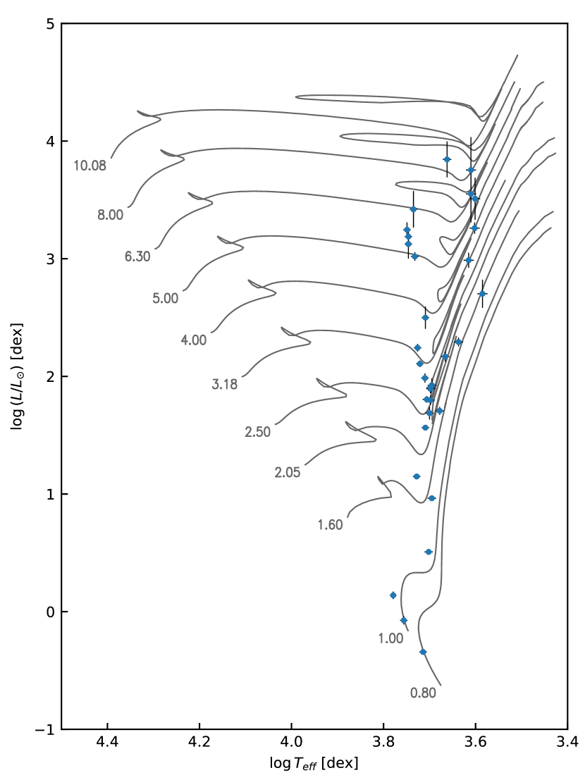
Figure 1: Grid of evolution tracks with solar metallicity for different stellar masses in solar mass units. The grid was calculated using the Cambridge (UK) Eggleton code in its version described and tested by Pols et al. (1997) and Pols et al. (1998).

3.4 Test with Gaia FGK Benchmark Stars

The Gaia FGK Benchmark Stars (GBS onwards, Jofré et al. (2014), Blanco-Cuaresma et al. (2014a) Heiter et al. (2015), Jofré et al. (2015), Hawkins et al. (2016), Jofré et al. (2017)) is a high resolution and high S/N library of a set of calibration star spectra. This library constitutes a set of very well-known stars especially convenient for spectral analysis assessments. It covers a wide range in effective temperature (3500 to 6600 K), surface gravity ($0.50$ to $4.60$ dex) and metallicity ($-2.70$ to $0.30$ dex). In addition, the stellar parameters of the set was mainly obtained from methods independent of spectroscopy.

We used four well-know stars from the GBS, $\delta$ Eri (HD23249), $\alpha$ Tau (HD 29139), Arcturus (HD 124897) and the Sun, to test the reliability of our method, as well as to see, if the use of TIGRE-HEROS spectra might somehow affect our results for reasons based on any instrumental issues. Therefore, spectra of three different resolutions and S/N (see Blanco-Cuaresma et al. (2014a) and references therein) are tested with our script and line list, after downgrading their resolution to the one of TIGRE-HEROS, $R=20,000$. The spectra in the GBS cover a wavelength range from 4800 Å to 6800 Å. For a meaningful comparison, we cut both GBS and R-channel TIGRE-HEROS spectra down to the same range of 5800 Å to 6800 Å.

The tests allow us to prove the reliability of our iSpec script on spectra other than TIGRE-HEROS, as well as the use of our line list in Table 6. We performed tests for many scenarios, including different resolutions, added spectra or using just one, automatic determination of parameters, varying the initial parameters, different wavelength ranges, etc. However, for the purpose of this publication, we only present the results of the first two tests, since the other test results do not differ much.

Table 3 summarizes the test results for $T_{\text{eff}}$, $\log\,g$, and [Fe/H], comparing the outcome of our iSpec script for different resolutions. To test for any changes in the stellar parameter determination, whether we add or not several TIGRE-HEROS spectra, we used three spectra for each star with an average S/N $\geq 100$.

These tests prove the reliability and robustness of the physical parameters obtained from the spectral synthesis approach taken with our iSpec script, employed on different resolutions. Therefore, we consider the total uncertainty of stellar parameters with this method as: $T_{\text{eff}}=\pm 100$ K, $\log g=\pm 0.15$ dex and $\text{[Fe/H]}=\pm 0.15$.

Table 3: Comparison tests with Gaia FGK Benchmark Stars. The original resolution of spectra has been downgraded to $R=20,000$.

Star	Instrument	Resolution	Adda	$T_{\text{eff}}$	$\Delta T_{\text{eff}}$b	$\log g$	$\Delta\log g$b	[Fe/H]	$\Delta\text{[Fe/H]}$b
				[K]	[K]	[dex]	[dex]	[dex]	dex
$\delta$ Eri (HD 23249)	TIGRE-HEROS	20524	False	4969 (29)	15	3.60 (0.04)	-0.16	-0.01 (0.02)	-0.07
$\delta$ Eri (HD 23249)	TIGRE-HEROS	20524	True	4974 (25)	20	3.59 (0.03)	-0.17	0.00 (0.01)	-0.06
$\delta$ Eri (HD 23249)	UVES.POP	85000	False	4972 (7)	18	3.64 (0.01)	-0.12	0.05 (0.01)	-0.01
$\delta$ Eri (HD 23249)	HARPS	115000	False	4971 (7)	17	3.62 (0.01)	-0.14	0.04 (0.00)	-0.02
$\alpha$ Tau (HD 29139)	TIGRE-HEROS	20366	False	3805 (20)	-122	1.13 (0.03)	0.02	-0.36 (0.02)	0.01
$\alpha$ Tau (HD 29139)	TIGRE-HEROS	20366	True	3798 (16)	-129	1.16 (0.03)	0.05	-0.37 (0.01)	0.00
$\alpha$ Tau (HD 29140)	NARVAL	80000	False	3821 (8)	-106	1.25 (0.02)	0.14	-0.27 (0.01)	0.10
$\alpha$ Tau (HD 29141)	HARPS	115000	False	3838 (17)	-89	1.24 (0.03)	0.13	-0.30 (0.01)	0.07
Arcturus (HD 124897)	TIGRE-HEROS	20435	False	4341 (19)	55	1.60 (0.05)	-0.04	-0.57 (0.02)	-0.04
Arcturus (HD 124897)	TIGRE-HEROS	20435	True	4342 (15)	56	1.61 (0.04)	-0.03	-0.57 (0.02)	-0.04
Arcturus (HD 124897)	UVES.POP	80000	False	4338 (3)	52	1.67 (0.01)	0.03	-0.52 (0.00)	0.01
Arcturus (HD 124897)	HARPS	115000	False	4334 (5)	48	1.64 (0.02)	0.00	-0.50 (0.01)	0.03
Sun	TIGRE-HEROS	20501	False	5750 (41)	-22	4.43 (0.06)	-0.01	-0.05 (0.02)	-0.05
Sun	TIGRE-HEROS	20501	True	5743 (34)	-29	4.43 (0.04)	-0.01	-0.05 (0.01)	-0.05
Sun	UVES	78000	False	5758 (14)	-14	4.45 (0.02)	0.01	-0.03 (0.01)	-0.03
Sun	HARPS	115000	False	5756 (12)	-16	4.44 (0.01)	0.00	-0.02 (0.01)	-0.02

• Adding three TIGRE-HEROS spectra.

• Differences with values in Gaia FGK Benchmark Stars library.

4 The Ca ii emission line widths of interest and their measurements

4.1 Formation of the Ca ii K emission line and where to take its width

The very cores of the Ca ii H&K lines are of such huge optical depth, that they provide one of very few windows into the chromospheres of cool stars. While most line cores in the optical spectrum reflect the physical conditions of the upper photosphere, the Ca ii doublet allows us to trace the temperature structure beyond its minimum at the base of the chromosphere, well into the rise, which is manifested by the Ca ii H&K line core reversals into emission. An early, extensive review of the chromospheric physics learned from this doublet was given by Linsky & Avrett (1970), and recent reviews are by Linsky (2017) and Ayres (2019). The focus is usually on the K line, often omitting its twin, in order to avoid any confusion which may arise from the overlap of the Ca ii H line with the hydrogen H_ϵ line.

Since Ca ii is more easily ionized than Mg ii and hydrogen, its formation does not reach into the increasingly warmer, uppermost chromosphere. There, magnetically dominated phenomena like prominences make the interpretation of, for example, H_α much more difficult. The K-lines reversal, its K2 emission, further shows a self-reversal (K3), which however must not be interpreted in terms of a temperature profile. Rather, this reversal is the product of extreme NLTE photon line scattering and geometrical distribution in the higher chromospheric layers – therefore much more prominent in luminous giants with their larger chromospheric extent. Hence, for a physical understanding of the lower chromosphere, our interest must be aimed on the outer proportions of the K2 chromospheric emission profile.

Consequently, Wilson & Bappu (1957) based their empirical relation between the chromospheric Ca ii K emission line width and visual absolute magnitude $M_{\text{V}}$ on their measurements of $W_{0}$ – chosen simply for the benefit of the best measurement precision, when taken as the positions of the outer edges of the calcium emission features. This is particularly true for measurements on photographic plates, as used in those days. Using the same spectrograms of Wilson & Bappu (1957), Lutz (1970) finally shows that the width at half intensity of the K emission line peak of Ca ii is better correlated with $M_{\text{V}}$ unlike the original method used by Wilson & Bappu (1957). Those peaks are also known as K2. Dealing with noisy spectra, the half-peak points are relatively well defined on the steep flanks of even a noisy emission line.

By contrast, the foot-points of the broad photospheric absorption line (K1) to either side of the chromospheric emission are not so well defined, especially in a noisy spectrum, because the deepest point in a shallow depression is ambiguous. But these K1 points are of theoretical significance: They are formed right at the base of the chromosphere, in the temperature-minimum. Assuming the source function there is still dominated by the Planck function, the minimal spectral flux observed in these deepest points of the K line on either side of the chromospheric emission reveals the physical conditions in temperature minimum.

However, as pointed out and illustrated by Shine et al. (1975) (see their Fig. 1), the exact distance and depths of these K1 points depends a lot on partial redistribution (PRD) effects on the K2 wings – becoming considerable, given the large number of photon line scattering events in this strong line prior to each escaping photon. PRD effects further increase with the larger chromospheric column densities in the more luminous giants. In that respect, Shine et al. (1975) already made it clear, that not considering PRD can lead to significant underestimates of the temperature in the temperature-minimum. Likewise, we conclude from their Fig. 1 that PRD and stellar gravity impact on the relation between $W_{0}$, O.C. Wilson’s half-maximum width, and the distance between the K1 points of the chromospheric emission line profile, hereafter referred to as $W_{1}$.

In their layout of a density-broadening explanation of the Wilson-Bappu effect – by the very numerous chromospheric absorption and re-emission events preceding each photon reaching the observer – Ayres et al. (1975) refer to the emission line width as taken between these two K1 foot points (i.e., $W_{1}$), simply for its significance by characterizing the base of the chromosphere. In assuming (without saying), as a first-order approximation, homologous emission line profiles across the giant branch, their explanation of the Wilson-Bappu effect, based on the theoretical arguments involving $W_{1}$, is implied to be true for O.C. Wilson’s $W_{0}$ as well.

However this simplification is not entirely true, as the theoretical work of Shine et al. (1975) already predicted, and as our measurements confirm below. In particular, when looking at lower gravities, $W_{1}$ starts to grow a bit faster that $W_{0}$. Because we are seeking a more precise comparison of theory with observation, this detail needs to be considered as well – which to our knowledge was never done before. The reason for that may simply stem from the difficulty to measure $W_{1}$. Hence, we here present our method to determine well both these line widths, handling well the presence of noise on the observed emission line profile, and used them here consistently for the whole sample.

4.2 Measuring the widths of the chromospheric Ca ii K emission line

The best way to use all information in an observed line profile with noise, is to empirically represent the whole profile by a best-fit analytical function, and then derive key quantities from that function. This approach avoids dependence on local noise effects, a particular advantage for measuring the shallow K1 minima by the foot points of the chromospheric emission, defining $W_{1}$ – provided, the representative function covers them well, too.

The physical features of the K emission line of Ca ii, however, are difficult to match by the types of profiles mostly used elsewhere in the analysis of spectral lines: Gaussian, Lorentzian, or a convolution of both, called Voigt profile. Lutz (1970) shows for the simplest case of a Ca ii K emission line, which does not have central self-absorption, that even there fitting a Lorentzian profile does not match correctly neither the wings of the line, nor the region of the peak. On the other hand, while a Gaussian fit matches better the line wings, it cannot represent the peak area either, because it is wider than the wing-matching Gaussian function. To fully consider the additional complexity of chromospheric Ca ii emission line profiles with central self-absorption, as required by this work, none of those three profiles are remotely adequate, and their use would only result in totally incorrect line width measurements.

To measure the width of the K emission line of Ca ii in the spectra of our stellar sample, we wrote a dedicated code, Half-Intensity Emission Width (HIEW v4.0), developed in C++. Our script HIEW works along a routine, which involves five main stages: (1) reading the configuration file and spectrum; (2) K-line representation by cubic splines to reduce variations caused by electronic noise in the spectrum; (3) determination of the minima and maxima in each of blue B and red R peaks of the K-line profile; (4) determination of the half peak intensity level, based on the average of the B and R peak intensity; (5) calculation of $W_{0}$ as the half-intensity emission width, and $W_{1}$ as the foot point separation of the representative emission line profile spline function.

In the observed spectrum, the real emission line profile is folded with the instrumental profile, and in this way the observed line is broadened by the limited spectral resolution. The instrumental profile width of TIGRE-HEROS is a function of wavelength and the instrumental FWHM in the Ca ii K line region is $\sim$ 0.19 Å (Schmitt et al. (2014), Czesla (2014)). However, the way of correction of the measured K-line widths by the instrumental profile width is a delicate matter, and has been discussed in detail already by Lutz (1970).

To consider in more detail the effects of the TIGRE-HEROS resolution in our measurements, we simulated an emission K line-profile using, as a first approximation, a sum of analytical functions (gaussian, voigt and both) even when, as Lutz (1970) clearly showed, the complexity of chromospheric Ca ii emission line profiles does not adequately fit any of these analytic functions. However, our tests showed that the use of two gaussian functions - with positive amplitude to fit the emission (K2) and negative amplitude to fit the autoabsorption (K3) - appears to match sufficiently well a number of representative cases of observed emission K line-profiles of our sample.

In a first step, we normalized the observed emission line by a cubic spline fitting of the Ca ii absorption. Then, we convoluted a simulated profile with the instrumental line profile (ILP) of TIGRE-HEROS and, by an RMS criterion, we improved recursively the analytical parameters of the functions considered. After 30 iterations the convolution of the simulated profile converges with the observed line profile. Fig. 5 shows the effect of the TIGRE-HEROS resolution in a simulated emission line for HD 205435 and the comparison with a observed Ca ii K emission line. As we could have expected, the maximum, and half maximum points of the simulated and observed line profiles differ. Nevertheless, the difference of $W_{0}$ line widths for both K line-profiles are within the instrumental error ($\sim$ 0.11 Å, equivalent to the standard deviation of TIGRE-HEROS’ instrumental line-profile close to the K-line of Ca ii).

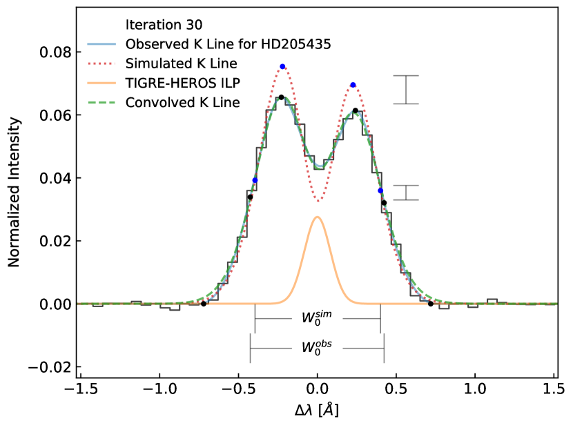
Figure 5: Simulation of the normalized Ca ii K emission line for HD 205435. We used a sum of two gaussian functions to simulated a K line profile (dotted red line) without the effect of the instrumental line profile of TIGRE-HEROS (solid orange line). The convolution between the simulated K emission line and instrumental line profile (dashed green line) fits well enough to the observed K emission line for HD 205435. Points mark the minimum, maximum, and half-maximum of the simulated (blue dots) and observed (black dots) line profiles. In the right part, we show the differences of the maximum averages and half-maximum averages. In the bottom part, we show the $W_{0}$ for simulated and observed emission line.

The two extremes, to subtract the instrumental resolution linearly, or in quadrature, are correct only if either both the instrumental profile and the line profile are lorentzian functions, or in the latter case, gaussians. But the K2 emission line shape is clearly neither, as mentioned above, and in the case of the HEROS spectrograph, the line profile is not gaussian (see Czesla (2014)). If anything, then the economic coverage of the nominal spectrograph resolution by only three pixels and the scattering characteristics in the fiber-feed may enhance the wings of the effective instrumental profile and bring it closer to a lorentzian function.

As already studied by Lutz (1970), the choice of this correction does matter a little bit, as it systematically affects the narrower lines more. We tested both approaches and find a maximum difference of 0.02 in the gravity exponent. In addition, the difference of widths of simulated, linear and quadrature subtraction are within the instrumental error of TIGRE-HEROS. However, given the analysis above, neither case is a priory a choice more justifiable than the other. Interestingly, O. C. Wilson always used the simple linear subtraction, and the detailed revision of his measurements by Lutz (1970) showed that it seemed to be more consistent than a trial with a subtraction in quadrature. Apparently, and by coincidence, another detail of the measuring process comes in to compensate any theoretical offset: washed-out (by limited resolution) narrower lines tend to be measured, effectively, further down than broad lines, when aiming at the 50 per cent level of the observed (and so broadened) profile. Hence, we settled for the simple linear correction method to arrive at our true widths of the Ca ii K emission line. The appendix B contains the line width measurements, and Table 4 summarizes these results for the whole stellar sample.

Table 4: Width measurements of the K emission line of Ca ii.

Star	$W_{0}$a	$W_{0}$b	$\log W_{0}$c	$W_{1}$a	$W_{1}$b	$\log W_{1}$c
	[Å]	[km/s]	[dex]	[Å]	[km/s]	[dex]
HD 8512	0.72	55	1.74 (0.07)	1.14	87.18	1.94 (0.04)
HD 10476	0.31	24	1.37 (0.16)	0.72	55.12	1.74 (0.07)
HD 18925	0.80	61	1.78 (0.06)	1.16	88.55	1.95 (0.04)
HD 20630	0.36	27	1.43 (0.14)	0.95	72.07	1.86 (0.05)
HD 23249	0.40	30	1.48 (0.12)	0.62	47.34	1.68 (0.08)
HD 26630	1.81	138	2.14 (0.03)	2.50	190.67	2.28 (0.02)
HD 27371	0.79	60	1.78 (0.06)	1.32	100.46	2.00 (0.04)
HD 27697	0.71	54	1.73 (0.07)	1.16	88.55	1.95 (0.04)
HD 28305	0.73	56	1.74 (0.07)	1.17	89.47	1.95 (0.04)
HD 28307	0.73	56	1.74 (0.07)	1.15	87.64	1.94 (0.04)
HD 29139	0.93	71	1.85 (0.05)	1.67	127.48	2.11 (0.03)
HD 31398	1.17	89	1.95 (0.04)	2.11	160.45	2.21 (0.02)
HD 31910	1.94	148	2.17 (0.03)	2.60	198.46	2.30 (0.02)
HD 32068	1.29	98	1.99 (0.04)	2.32	176.48	2.25 (0.02)
HD 48329	1.73	132	2.12 (0.03)	2.59	197.70	2.30 (0.02)
HD 71369	0.76	58	1.77 (0.06)	1.13	86.30	1.94 (0.04)
HD 81797	1.01	77	1.88 (0.05)	1.85	141.22	2.15 (0.03)
HD 82210	0.53	40	1.61 (0.09)	1.34	102.34	2.01 (0.04)
HD 96833	0.76	58	1.76 (0.07)	1.37	104.12	2.02 (0.04)
HD 104979	0.68	52	1.72 (0.07)	0.93	70.83	1.85 (0.05)
HD 109379	0.83	63	1.80 (0.06)	1.13	86.26	1.94 (0.04)
HD 114710	0.48	37	1.57 (0.10)	0.75	56.95	1.76 (0.07)
HD 115659	0.72	55	1.74 (0.07)	1.13	86.26	1.94 (0.04)
HD 124897	0.84	64	1.80 (0.06)	1.35	102.75	2.01 (0.04)
HD 148387	0.70	53	1.73 (0.07)	0.97	73.90	1.87 (0.05)
HD 159181	1.93	147	2.17 (0.03)	2.82	215.00	2.33 (0.02)
HD 164058	0.96	73	1.86 (0.05)	1.86	142.13	2.15 (0.03)
HD 186791	1.20	91	1.96 (0.04)	2.28	173.73	2.24 (0.02)
HD 198149	0.50	38	1.58 (0.10)	0.71	54.21	1.73 (0.07)
HD 204867	1.89	144	2.16 (0.03)	2.46	187.47	2.27 (0.02)
HD 205435	0.66	50	1.70 (0.08)	1.27	96.79	1.99 (0.04)
HD 209750	1.86	142	2.15 (0.03)	2.62	199.38	2.30 (0.02)

• The error of the line width measurements is equivalent to the standard deviation of TIGRE-HEROS’ instrumental line-profile close to K-line of Ca ii $\sim$ 0.11 Å.

• The error in km/s is equivalent to 8 km/s.

• Logarithmic values correspond to widths in km/s.

4.3 Are $W_{0}$ and $W_{1}$ analogous measurements of the Ca ii K emission line width?

As pointed out before, Ayres et al. (1975) and also Cram & Ulmschneider (1978) compared and proposed empirical width-luminosity correlations, referring to the Ca ii K₁ minimum features, which means the $W_{1}$ widths, not O.C. Wilson’s $W_{0}$. However, in his work Ayres (1979) argues that $W_{0}$ should be, much like $W_{1}$, proportional to $g^{1/4}$, too. That would be the case, e.g., if the emission line profiles were homologous. However, we want to revise this element of the comparison of theory with observation as well. Consequently, we compared the $W_{0}$ and $W_{1}$ widths to see, whether they are indeed analogous measurements of the chromospheric Ca ii K line emission width, using our above described measurement method (see section 4.2)

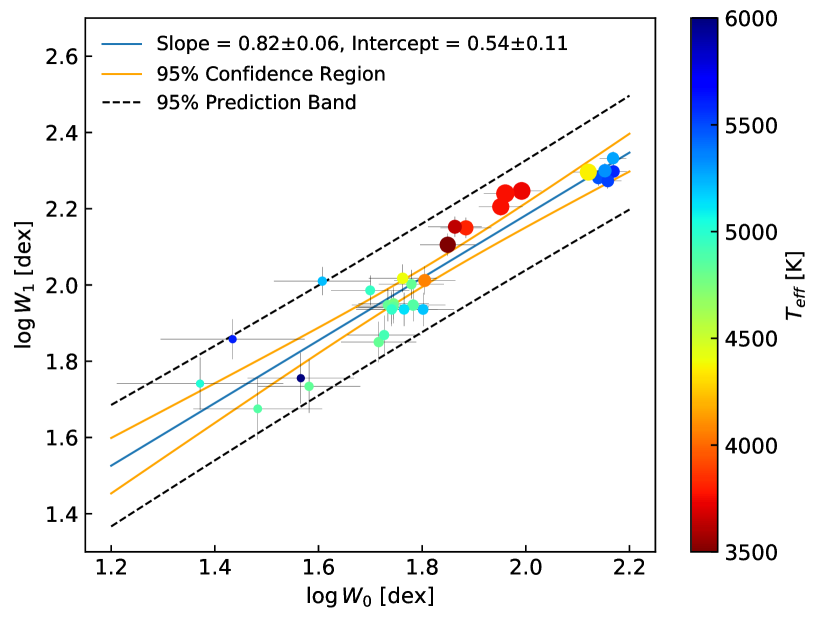
Figure 6: Comparison of line width measurements $\log W_{1}$ vs $\log W_{0}$ of the Ca ii K emission line for the stellar sample. We used the logarithmic values of widths in km/s. The blue line corresponds to a linear fit. The color code represents the effective temperature, and the point-size represents the surface gravity with larger points for lower gravities.

Using the width measurements of the Ca ii K emission line listed in Table 4, we compare and correlate $W_{1}$ with $W_{0}$ for our stellar sample. Fig. 6 shows this comparison, resulting in a linear least squares fit with a high Pearson’s correlation coefficient of 0.934. The best relation for $W_{1}$ versus $W_{0}$ is

$$\log W_{1}=(0.82\pm 0.06)\log W_{0}+(0.54\pm 0.11).$$ (2)

This relation is not far from what one may expect of homologous emission line profiles (implying an exponent of 1.0), however it clearly proves that $W_{1}$ and $W_{0}$ scale differently over our sample. The effect is significant and must be taken into consideration by the comparison of theory with observation, see section below, in particular for the relation of line width with gravity.

5 Gravity and temperature dependence: observation versus theory

The relation between the width of the Ca ii K emission line and the stellar parameters, i.e. effective temperature and surface gravity, has been studied by a number of authors during the last decades (Reimers (1973), Neckel (1974), Ayres et al. (1975), Ayres (1979), Lutz & Pagel (1982), Park et al. (2013)). The work of Ayres et al. (1975) demonstrated, how the Wilson-Bappu effect can be derived from of the relation of the chromospheric Ca ii column density $N$ with gravity $g$, assuming hydrostatic equilibrium at the bottom of the chromosphere. $N$ in turn reflects on how the line width grows with lower gravity, by simple density-broadening – the migration of the photons into the line wings after multiple absorption and re-emission processes. Assuming also that the mean continuum optical depth in the stellar temperature minimum is relatively independent of surface gravity, Ayres et al. (1975) arrived at the simple relation $W_{1}\propto{A_{\text{met}}}^{1/4}g^{-1/4}$, where $A_{\text{met}}$ is the abundance of easily ionized metals relative to hydrogen. The simplification of the opacity problem, required to derive the above relation, was later supported by more detailed arguments, given in Ayres (1979) and Ayres (2019). A key point is, irrespective of, e.g., the relative proportions of H^- and line opacities in each chromosphere, that all relevant contributions to the opacity are controlled by the electron density in the same way.

We deliberately avoided studying the possible metallicity dependence, by the choice of a sample of mostly solar abundance, in order to have fewer ambiguity on the gravity dependence and to test the theoretical approach as such. A dependence of $W_{1}$ on $T_{\text{eff}}$ was still ignored by Ayres et al. (1975) because their initial stellar sample did not spread much over that parameter, only in gravity, but was then taken into consideration soon after by Ayres (1979). In consequence, the line broadening appears to depend on both, gravity and effective temperature. The latter effect is based on the ionization ratio of Ca i:Ca ii, consequently reducing the Ca ii column density in the coolest chromospheres (comparing stars of same surface gravity). Still this is of secondary nature because the range of effective temperatures of cool stars with chromospheres is quite limited, while gravity covers more than four orders of magnitude.

There is now a problem with any empirical assessment of the line width relation, simultaneously with both these parameters: cross-talk from a mismatch of the effective temperature affecting the gravity term. That interrelation is caused by the orientation of the giant branches in the HR diagram: the coolest giants are also mostly those with the highest luminosity and, consequently, lowest gravity. Hence, to empirically evaluate the theoretical reasoning of Ayres et al. (1975) by means of the gravity term of the emission line width, one must get the temperature term right as well.

To test the interpretation of the Wilson-Bappu effect by Ayres et al. (1975) and Ayres (1979), we derived the width correlation of the Ca ii K emission line with surface gravity and effective temperature in our sample, for both measurements, $W_{0}$ and $W_{1}$, using simple power-law relations in their logarithmic form:

$$\log W=\alpha\log\,g+\beta\log T_{\text{eff}}+C.$$ (3)

where $\alpha$, $\beta$ and $C$ are fitting constants. Table 5 shows the results for these values when we apply equation 3 to $W_{0}$ and $W_{1}$.

Table 5: Results for the gravity and temperature dependence of the WBE considering different measurements of the K emission line of Ca ii.

Width	$\alpha$	$\beta$	$C$	$\chi^{2}$
$W_{0}$	-0.279 (0.011)	2.93 (0.22)	-8.3 (0.8)	0.0360
$W_{1}$	-0.220 (0.020)	1.8 (0.4)	-4.1 (1.4)	0.1040
$W_{1}^{\prime}$	-0.229 (0.009)	2.41 (0.18)	-6.3 (0.7)	0.0216

Based on the best $\chi^{2}$, we observe that $W_{0}$ has a better correlation with gravity and temperature than $W_{1}$ for our stellar sample. However, this can be explained by the better definition of the former on the flanks of line profile. And as we showed in subsection 4.3, there is a clear relation between both widths, where $W_{0}$ rises a bit faster than $W_{1}$ (see equation 2). Therefore, the relation of $\log\,W_{1}$ has a smaller power with $\log\,g$ than $\log\,W_{0}$.

We may also convert $W_{0}$ into $W_{1}$ values, using equation 2, in order to circumnavigate the larger uncertainties of individual $W_{1}$ values. We tested the dependence of these converted values $W_{1}^{\prime}$ with gravity and temperature in the same way as before and found that their correlation got two times better than $W_{0}$, based on the respective minimal $\chi^{2}$ sums. In addition, the gravity exponent calculated with $W_{1}^{\prime}$ is the closest to the theoretical prediction of Ayres et al. (1975). This is pictured in Fig. 7 and Fig. 8, showing the direct dependence of $\log\,W_{1}^{\prime}$ with $\log\,g$, as well as $\log\,T_{\text{eff}}$, subtracting the respective other contribution.

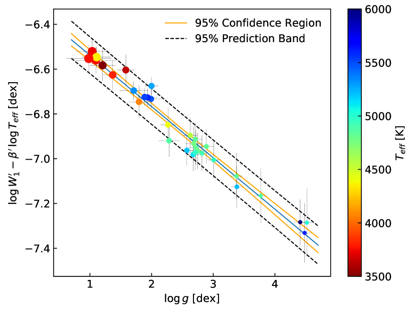
Figure 7: Dependence of $W_{1}^{\prime}$ on $\log\,g$ by subtracting the temperature contribution. The blue line corresponds to a linear fit. The color code represents the effective temperature, and the point-size represents the surface gravity, using larger points for lower gravities.

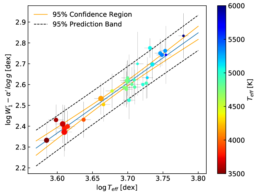
Figure 8: Dependence of $W_{1}^{\prime}$ on $\log\,T_{\text{eff}}$ by subtracting the gravity contribution. The blue line corresponds to a linear fit. The color code represents the effective temperature, and the point-size represents the surface gravity with larger points for lower gravities.

6 Conclusions

We developed and demonstrated a consistent analysis, applied uniformly on a representative stellar sample, for which we obtained good S/N TIGRE spectra of the moderately high spectral resolving power of $R\sim 20,000$. The new Gaia EDR3 parallaxes allowed us to calculate precise, parallax-based gravities, in combination with stellar mass estimates based on HRD-position matching evolution tracks. That approach facilitated the assessment of effective temperatures by means of spectral synthesizing, as we were able to exclude false solutions with erroneous gravities.

Furthermore, with the help of our here presented measurement technique for the chromospheric Ca ii K emission line width, we found that the width used by O.C. Wilson, $W_{0}$ (the width at half-peak intensity), and the width of theoretical significance, $W_{1}$ (the K₁ minima separation, originating in the temperature minimum at the very bottom of the chromosphere), do not scale 1:1 across the HRD, but are related to each other by $\log W_{1}=0.82\log W_{0}+0.53$. Hence, chromospheric emission lines are not exactly homologous over a wider range of gravity. Therefore, the relation between $W_{0}$ and $W_{1}$ is required to extend the empirical Wilson-Bappu effect, based on $W_{0}$, to a relation of the line width with physical parameters such as gravity and effective temperature, as predicted by theory for $W_{1}$.

This distinction and the above described consistent approach to the physical parameter assessment for our sample stars, enables us to test the theoretical explanation of Ayres et al. (1975) and Ayres (1979), in particular by comparing the empirical findings to their predicted gravity dependence. In fact, ignoring the difference between the two emission line widths leads to a much worse agreement of theory with observation.

In conclusion, we confirm the dependence on gravity proposed by Ayres et al. (1975) and Ayres (1979), suggesting that the Wilson-Bappu effect is indeed a line saturation and photon redistribution effect, driven by the growing column densities in giants with lower gravities. That same interpretation provides a straight-forward explanation for the temperature term as well, namely the effect of the Ca ii:Ca i ionization balance. Even though it is difficult to quantify, because (i) the relevant temperature of the line-forming layers of each chromosphere cannot so easily be related to the effective temperature of the respective stellar photosphere underneath, and (ii) because of NLTE effects in any chromospheric ionization balance, the intuitive understanding is that cooler stars have a larger fraction of neutral Ca in their chromospheres, resulting in a reduced Ca ii column density. This explains the positive sign of the temperature exponent, while the substantial effect over a relatively small temperature range calls for a large value – as observed.

This nice agreement of our empirical study with the theoretical predictions of Ayres et al. (1975) also suggests the validity, at least to a good degree, of their assumption of hydrostatic equilibrium at the base of the chromosphere – at least for stars, that are not overly active. In those cases, the chromospheric structure is not dominated by magnetic energy density and its dynamic fine structure. This is good news: chromospheric physics may not be entirely hopeless – after all, some approximations do appear to be reasonable. At least, this is our interpretation of the meaning of the Wilson-Bappu effect and the agreement obtained with simple chromospheric physics.

Data Availability

The data underlying this article are available in the article.

Appendix A Pseudo-continuum readjustment and line selection for synthezising procedure with iSpec

A.1 Guided readjustment of the pseudo-continuum

To find suitable continuum sections, which are needed to guide the readjustment of the pseudo-continuum of the observed spectrum, ideally at the value of 1.0, we used a synthetic spectrum that matches the observed spectrum reasonably well. To produce it, the initial values of $T_{\text{eff}}$, $\log g$ and [Fe/H] were set to the averages of the respective entries in the PASTEL catalogue. Furthermore, the resolution of the synthetic spectrum was set to the one of the TIGRE-HEROS target spectrum ($R\sim 20,000$), and the projected rotation velocity $v\sin i$ was fixed at the small value of 1.6 km/s. This is a reasonable choice for giants, as well as for aged and relatively inactive main sequence stars, which form our sample. Individual differences of a few km/s in this rotation rate cannot be resolved by TIGRE-HEROS spectra, anyway.

At this point, another choice was required, namely for the initial values of micro and macro turbulent velocities. Despite these being below the resolution limit of TIGRE-HEROS spectra, their choices make subtle but systematic differences in the $\chi^{2}$ sums of later best-fit solutions. Therefore, in the final synthesizing of the physical parameters (see below), the turbulence values are allowed to be refined, see Table 1. But for the initial model spectrum required here only to define suitable continuum sections, we needed reasonable fixed values.

Initially, we tested the macro and micro-turbulence velocities, $v_{\text{mac}}$ and $v_{\text{mic}}$, used for the models of the phoenix library (Husser et al., 2013), which give reasonably realistic spectra for stars with solar abundances, over a range of effective temperatures and surface gravities. Therefore, like (Husser et al., 2013), we first fixed the macro-turbulence parameters at twice the micro-turbulence values. However, after several tests with well-studied stars (see subsection 3.4), we refined the initial choices of macro-turbulence velocity $v_{\text{mac}}$ by the following empirical representation, according to the findings in main sequence stars by Ryabchikova et al. (2016), while still using the micro-turbulence values of Husser et al. (2013) in this step:

$$v_{\text{mac}}=\left\{\begin{array}[]{ll}2.00v_{\text{mic}}&\textup{if }\log g\leq 2.0\\ 3.00v_{\text{mic}}&\textup{if }2.0<\log g<3.75\\ 3.75v_{\text{mic}}&\textup{if }\log g\geq 3.75.\end{array}\right.$$ (4)

In this so-defined, representative synthetic spectrum, we then selected continuum sections according to the following criteria: (1) Maximum standard deviation from 1.0 of 0.1 per cent, and (2) minimum size of the region equivalent to FWHM of the instrumental profile of TIGRE-HEROS ($\sim$ 0.35 Å in the center of R-channel, $\sim$ 0.23 Å in the centre of B-channel). (3) To avoid confusion, spectral regions with abundant telluric lines were also discarded (Catanzaro, 1997).

These continuum sections were finally used to readjust the observed stellar pseudo-continuum, employing the iSpec algorithm designed for this. According to Blanco-Cuaresma et al. (2014b), this subroutine applies a median and maximum filter with different window sizes. The former smooths out the noise in the continuum, while the latter ignores slightly smaller fluxes, which rather belong to shallow absorption lines – i.e., the continuum may effectively be placed slightly above or below the simple flux average in the respective continuum section, depending on the values of those parameters. Then, this algorithm applies a third-degree spline, assigning one node every 20 Å only within these selected continuum regions. This procedure is repeated recursively to different median and maximum filters, ten steps for each one from 0.1 Å to 1.0 Å for the first, and 1.5 Å to 15 Å for the last one. A total of up to 100 possible normalizations are calculated.

The script finds the residuals between the synthetic and observed spectrum, and calculates the RMS only in the continuum regions. The readjusted spectrum with the best RMS is finally chosen. Finally, a second fine-tuning normalization is applied to the observed spectrum. Using again the continuum sections, this time as a template in the observed spectrum, the iSpec script further improves the normalization by the use of a median filter equal to the instrumental profile width of TIGRE-HEROS. As a whole, this guided continuum readjustment procedure improves the original normalization of the observed spectrum significantly, because the former can be mislead by agglomerations of absorption lines.

A.2 Selection of representative lines for synthesizing procedure

We selected a representative, reliable subset of lines for the synthesizing procedure, aiming on small $\chi^{2}$ minima, less impacted by line blends or mismatching atomic line strengths ($f$-values). For our sample stars, we based that selection on the following criteria: (1) the S/N in each line must be greater than 5 times; (2) a cross correlation is undertaken between the information of the Vienna Atomic Line Data Base (VALD) (Piskunov et al., 1995) and the observed lines, avoiding differences in wavelength larger than the width of the instrumental profile of TIGRE-HEROS ($\sim 0.35$ Å); (3) lines within spectral regions known to host many telluric lines are discarded; (4) were the observed line strength disagrees with the atomic data of the VALD list, or would even be zero according to the synthetic spectrum, such lines are discarded (see below).

We applied these criteria to a good solar spectrum, taken by TIGRE-HEROS, using a strategy similar to the line-by-line differential approach of Blanco-Cuaresma (2019), that is: a line can be considered good, when synthesizing arrives at a close-to-solar abundance (i.e. reasonably close to zero). After several tests, if a spectral element has more than 20 lines, we considered an abundance mismatch-margin of $\pm 0.15$ dex, otherwise accepted a margin of $\pm 0.50$ dex. Hence, lines producing an error larger than 0.50 dex are discarded. This tolerated metallicity mismatch, reflecting atomic data mismatches of the line list, is a compromise between quantity and quality of the selection. By this approach, only lines from iron peak elements (iron, chromium, nickel) and alpha elements (silicon, calcium, titanium) would qualify. For the here required solar reference model, we used the solar parameters to $T_{\text{eff}}=5772$ K, $\log g=4.44$ dex and $\text{[M/H]}=0.00$ dex. Again the initial $v_{\text{mic}}$ was determined using the phoenix library, $v_{\text{mac}}$ with equation 4, and $v\sin i$ was fixed to 1.6 km/s.

From this process, a total of 202 lines were selected for the R-channel spectra of HEROS (covering 5800 to 8700 Å). The final line list is shown in Table 6. In the same way of Blanco-Cuaresma (2019), these lines are not blindly used on the observed spectra. Before starting the parameter synthesizing process, the script checks if each of these lines exists in the target spectrum, and using a gaussian fit, then applies the equivalent width criterion as stated above, before including the line in the process. According to our tests, these lines worked well enough for our sample from main sequence stars to supergiants (see subsection 3.4).

Table 6: List of lines selected for use with the iSpec script.

$\lambda_{0}$	$\lambda_{\text{blue}}$	$\lambda_{\text{red}}$	Note
[nm]	[nm]	[nm]
580.52548	580.48018	580.55266	Ni 1
580.57078	580.55266	580.61608	Fe 1
580.67044	580.61608	580.73386	Fe 1
580.92412	580.84258	581.01472	Fe 1
581.47677	581.43147	581.55831	Fe 1
581.63079	581.57643	581.67609	Fe 1
583.16193	583.10757	583.21629	Ni 1
583.83236	583.78706	583.89578	Fe 1
584.70212	584.64776	584.75648	Ni 1
584.81084	584.75648	584.85614	Fe 1
585.74402	585.64436	585.81650	Ca 1
585.96145	585.90709	586.04299	Fe 1
586.64095	586.58659	586.68625	Ti 1
586.75873	586.68625	586.79497	Ca 1
587.32045	587.26609	587.35669	Fe 1
592.77455	592.72925	592.81079	Fe 1
593.01916	592.98292	593.07352	Fe 1
593.46310	593.41780	593.51746	Fe 1
595.27510	595.21168	595.37475	Fe 1
596.58879	596.51631	596.63409	Ti 1
597.85718	597.82094	597.92966	Ti 1
598.48232	598.43702	598.58198	Fe 1
599.13464	599.09840	599.16182	Fe 2
599.67824	599.62388	599.70542	Ni 1
600.72919	600.68389	600.75637	Ni 1
600.79261	600.75637	600.81979	Fe 1
604.20822	604.11762	604.28070	Fe 1
605.36789	605.31353	605.47661	Ni 1
605.60345	605.55815	605.67593	Fe 1
606.54569	606.50039	606.62723	Fe 1
608.41204	608.33956	608.45734	Fe 2
608.52076	608.45734	608.57512	Fe 1
608.62948	608.57512	608.72008	Ni 1
609.11872	609.07342	609.14590	Ti 1
609.36334	609.32710	609.39958	Fe 1
609.82539	609.78915	609.94317	Fe 1
610.26933	610.24215	610.30557	Ca 1
610.32369	610.30557	610.41429	Fe 1
612.21722	612.12662	612.30782	Ca 1
612.49808	612.42560	612.56150	Si 1
612.62492	612.56150	612.67928	Ti 1
612.78800	612.71552	612.85142	Fe 1
612.89672	612.85142	612.94202	Ni 1
613.17758	613.08698	613.26818	Si 1
613.66682	613.61246	613.73024	Fe 1
614.24665	614.21947	614.29195	Si 1
614.50033	614.44597	614.58187	Si 1
614.78119	614.69965	614.82649	Fe 1
614.92615	614.88085	614.97145	Fe 2
615.16171	615.10735	615.20701	Fe 1
615.76873	615.70531	615.85933	Fe 1
616.13113	616.10395	616.16737	Ca 1
616.22173	616.16737	616.29421	Ca 1
616.35763	616.29421	616.42105	Ca 1
616.53882	616.49352	616.59318	Fe 1
616.64754	616.59318	616.73814	Ca 1
616.90122	616.81968	616.92840	Ca 1
616.95558	616.92840	617.00994	Ca 1
617.05524	617.00994	617.16396	Fe 1
617.33610	617.27268	617.38140	Fe 1

Table 7: continued

List of lines selected for use with the iSpec script. $\lambda_{0}$ $\lambda_{\text{blue}}$ $\lambda_{\text{red}}$ Note [nm] [nm] [nm] 617.53542 617.45388 617.58978 Ni 1 617.68038 617.61696 617.78004 Ni 1 618.02466 617.97030 618.07902 Fe 1 618.35988 618.30552 618.42330 Fe 1 619.15715 619.04843 619.27493 Fe 1 619.54673 619.50143 619.60109 Si 1 620.03597 619.98161 620.08127 Fe 1 621.34060 621.28624 621.42214 Fe 1 622.02916 621.97480 622.04728 Ti 1 622.40062 622.33720 622.43686 Ni 1 622.67242 622.59088 622.71772 Fe 1 622.92610 622.85362 622.97140 Fe 1 623.00764 622.97140 623.02576 Ni 1 623.07106 623.02576 623.16166 Fe 1 623.73243 623.57841 623.78679 Si 1 623.84115 623.78679 623.89551 Fe 2 624.06765 623.95893 624.11295 Fe 1 624.38475 624.33945 624.41193 Si 1 624.62937 624.58407 624.69279 Fe 1 624.75621 624.69279 624.81057 Fe 2 625.25451 625.20921 625.31793 Fe 1 625.80717 625.77093 625.83435 Ti 1 625.87059 625.83435 625.91588 Ti 1 625.96118 625.91588 626.01554 Ni 1 626.10614 626.05178 626.16956 Ti 1 627.02120 626.95778 627.07556 Fe 1 627.12992 627.07556 627.16616 Fe 1 630.14689 630.09253 630.21031 Fe 1 631.14348 631.08912 631.18878 Fe 1 631.57836 631.56024 631.62366 Fe 1 632.21256 632.16726 632.23068 Ni 1 632.26692 632.23068 632.32128 Fe 1 633.00983 632.93736 633.04607 Cr 1 633.68027 633.62591 633.77087 Fe 1 633.89771 633.81617 633.97019 Ni 1 635.86372 635.81842 635.93620 Fe 1 636.28954 636.26236 636.38920 Fe 1 636.44356 636.38920 636.52510 Fe 1 636.64288 636.58852 636.69724 Ni 1 636.95092 636.86032 636.98716 Fe 2 637.13212 637.07776 637.20460 Si 2 637.82973 637.77537 637.92033 Ni 1 638.07435 638.01999 638.14683 Fe 1 638.46393 638.41863 638.50923 Ni 1 638.56359 638.50923 638.61795 Fe 1 639.26121 639.17061 639.28839 Fe 1 639.36087 639.28839 639.47865 Fe 1 640.00412 639.90447 640.08566 Fe 1 640.72892 640.63832 640.75610 Si 1 641.16380 641.04602 641.23628 Fe 1 641.49902 641.40842 641.59868 Si 1 641.68928 641.62586 641.73458 Fe 2 641.99732 641.90672 642.05168 Fe 1 642.13322 642.07886 642.20570 Fe 1 642.48655 642.42313 642.53185 Ni 1 643.08451 643.00297 643.13887 Fe 1 643.90897 643.83649 644.02675 Ca 1 644.97804 644.94180 645.09582 Ca 1 645.55788 645.52164 645.59412 Ca 1 645.63942 645.59412 645.67566 Fe 2

Table 8: continued

List of lines selected for use with the iSpec script. $\lambda_{0}$ $\lambda_{\text{blue}}$ $\lambda_{\text{red}}$ Note [nm] [nm] [nm] 646.26456 646.20114 646.31892 Ca 1 649.15469 649.11845 649.21811 Ti 2 649.38119 649.33589 649.41742 Ca 1 649.49896 649.41742 649.54426 Fe 1 649.65298 649.61674 649.66204 Fe 1 649.89760 649.84324 649.92478 Fe 1 649.96102 649.92478 650.05162 Ca 1 659.75484 659.69142 659.80920 Fe 1 660.91452 660.85110 661.01418 Fe 1 662.50001 662.44565 662.54531 Fe 1 662.75369 662.68121 662.79899 Fe 1 663.51473 663.46037 663.55096 Ni 1 663.97678 663.92242 664.04020 Fe 1 664.69252 664.65628 664.74688 Fe 1 666.11493 666.06057 666.16929 Cr 1 666.76725 666.70383 666.81255 Fe 1 667.80009 667.69137 667.85445 Fe 1 671.03449 670.98919 671.09791 Fe 1 671.62339 671.57809 671.66869 Fe 1 672.53845 672.49315 672.59281 Fe 1 672.66529 672.59281 672.75589 Fe 1 674.31420 674.23266 674.42292 Ti 1 675.01182 674.95746 675.07524 Fe 1 675.27456 675.20208 675.31985 Fe 1 677.23151 677.16809 677.30399 Ni 1 679.35154 679.27000 679.40590 Fe 1 680.68335 680.61993 680.74677 Fe 1 681.02763 680.97327 681.08199 Fe 1 682.85774 682.73996 682.93928 Fe 1 683.70032 683.61878 683.79998 Fe 1 683.98118 683.93588 684.02648 Fe 1 684.13520 684.02648 684.17144 Fe 1 684.20768 684.17144 684.23486 Ni 1 684.36170 684.31640 684.43418 Fe 1 685.51231 685.39453 685.64821 Fe 1 685.81129 685.76599 685.89283 Fe 1 686.24617 686.21899 686.32771 Fe 1 743.07931 743.01589 743.12461 Fe 1 744.30240 744.24804 744.38394 Fe 1 744.93660 744.85506 744.98190 Fe 2 745.39866 745.33524 745.46208 Fe 1 746.15063 746.09627 746.18687 Fe 1 746.23217 746.18687 746.29559 Cr 1 747.35561 747.31031 747.40997 Fe 1 748.19819 748.09853 748.27066 Fe 1 749.16760 749.10418 749.26726 Fe 1 750.60813 750.55378 750.66249 Fe 1 751.10643 750.92523 751.20609 Fe 1 752.27517 752.20269 752.36577 Ni 1 752.51073 752.44731 752.58321 Ni 1 754.18682 754.09622 754.24118 Fe 1 757.40311 757.35781 757.48465 Ni 1 758.38158 758.27286 758.46312 Fe 1 772.75974 772.68726 772.83222 Ni 1 774.55361 774.47207 774.61703 Fe 1 774.65327 774.61703 774.71669 Fe 1 774.82541 774.71669 774.86165 Fe 1 774.88883 774.86165 774.95225 Ni 1 775.11533 775.03379 775.20593 Fe 1 776.05757 775.99415 776.19347 Si 1

Table 9: continued

List of lines selected for use with the iSpec script. $\lambda_{0}$ $\lambda_{\text{blue}}$ $\lambda_{\text{red}}$ Note [nm] [nm] [nm] 780.78687 780.70533 780.85935 Fe 1 784.99975 784.90915 785.06317 Si 1 785.53429 785.47993 785.62489 Fe 1 846.84305 846.77057 846.96989 Fe 1 847.16920 847.07860 847.29604 Fe 1 848.19298 848.12050 848.26546 Fe 1 849.80565 849.46137 850.09557 Ca 2 851.40927 851.34585 851.46363 Fe 1 851.50893 851.46363 851.57235 Fe 1 851.83508 851.77167 851.89850 Ti 1 855.67651 855.59497 855.82147 Si 1 858.23142 858.13176 858.28578 Fe 1 859.59041 859.52699 859.65383 Si 1 859.70819 859.65383 859.78067 Si 1 859.88033 859.78067 859.97093 Fe 1 861.17591 861.11249 861.23932 Fe 1 862.16344 862.10002 862.22686 Fe 1 863.69457 863.65833 863.75799 Ni 1 867.47258 867.40916 867.65378 Fe 1 868.64131 868.54165 868.72285 Si 1 868.85875 868.72285 868.94935 Fe 1 869.94595 869.90065 869.98219 Fe 1

Appendix B Ca ii emission line width measurements of the stellar sample

We present the Ca ii emission line width measurements of the stellar sample with a fixed wavelength scale to comparison purposes. Fig. 9 shows the measurements for HD 8512, HD 10476, HD 18925, HD 20630, HD 23249, HD 26630, HD 27371 and HD 27697. Fig. 10 for HD 28305, HD 28307, HD 29139, HD 31398, HD 31910, HD 32068, HD 48329 and HD 71369. Fig. 11 for HD 81797, HD 82210, HD 96833, HD 104979, HD 109379, HD 114710, HD 115659 and HD 124897. Fig. 12 for HD 148387, HD 159181, HD 164058, HD 186791, HD 198149, HD 204867, HD 205435 and HD 209750. The blue line represents the fit using cubic splines, the dashed line is the half intensity of the peak and gray zone is the measurement uncertainty.

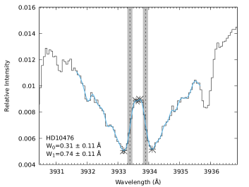
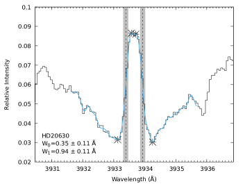
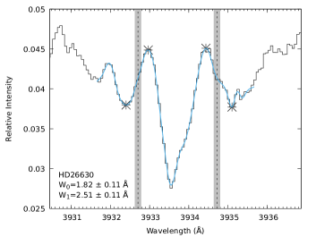
Figure 9: Ca ii emission line width measurements of HD 8512, HD 10476, HD 18925, HD 20630, HD 23249, HD 26630, HD 27371 and HD 27697.

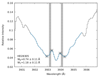
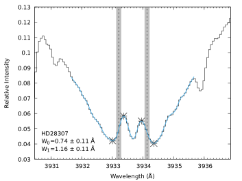
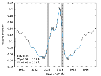
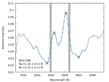
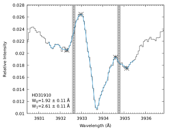
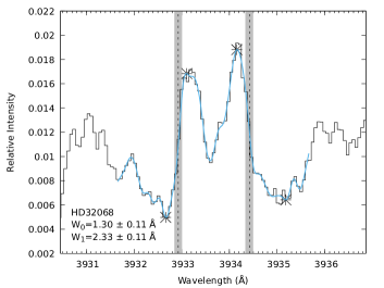
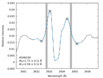
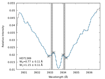
Figure 10: Ca ii emission line width measurements of HD 28305, HD 28307, HD 29139, HD 31398, HD 31910, HD 32068, HD 48329 and HD 71369.

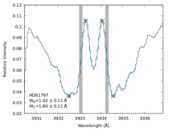
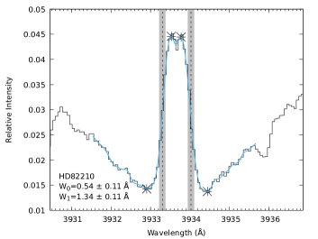
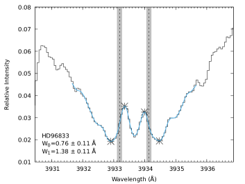
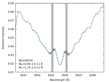
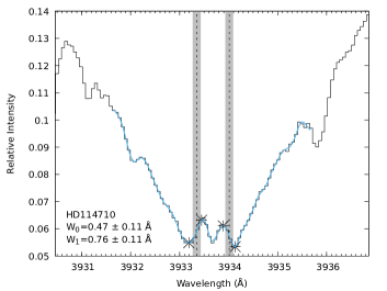
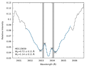
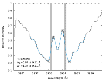
Figure 11: Ca ii emission line width measurements of HD 81797, HD 82210, HD 96833, HD 104979, HD 109379, HD 114710, HD 115659 and HD 124897.

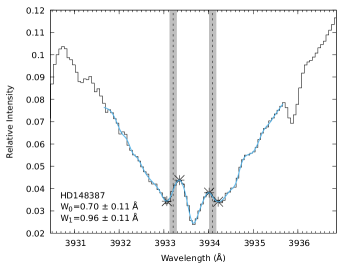
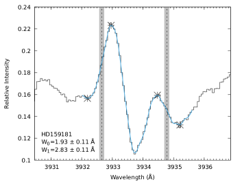
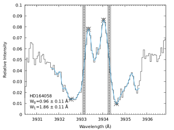
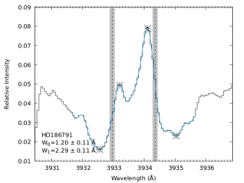
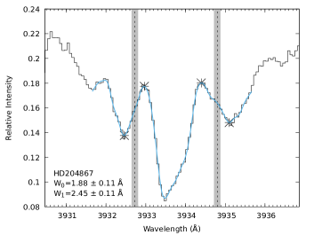
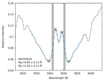
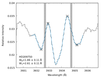
Figure 12: Ca ii emission line width measurements of HD 148387, HD 159181, HD 164058, HD 186791, HD 198149, HD 204867, HD 205435 and HD 209750.

References

- Alvarez & Plez (1997) Alvarez R., Plez B., 1997, A&A, 330, 1109
- Aurière et al. (2015) Aurière M., et al., 2015, A&A, 574, A90
- Ayres (1979) Ayres T. R., 1979, ApJ, 228, 509
- Ayres (2019) Ayres T. R., 2019, in , The Sun as a Guide to Stellar Physics. Elsevier, pp 27–57, doi:10.1016/B978-0-12-814334-6.00002-9
- Ayres et al. (1975) Ayres T. R., Shine R. A., Linsky J. L., 1975, ApJ, 195, L121
- Blanco-Cuaresma (2019) Blanco-Cuaresma S., 2019, MNRAS, 486, 2075
- Blanco-Cuaresma et al. (2014a) Blanco-Cuaresma S., Soubiran C., Jofré P., Heiter U., 2014a, A&A, 566, 1
- Blanco-Cuaresma et al. (2014b) Blanco-Cuaresma S., Soubiran C., Heiter U., Jofré P., 2014b, A&A, 569, A111
- Catanzaro (1997) Catanzaro G., 1997, Ap&SS, 257, 161
- Cram & Ulmschneider (1978) Cram L. E., Ulmschneider P., 1978, A&A, 62, 239
- Czesla (2014) Czesla S., 2014, Technical Report 1, The instrumental line-profile of TIGRE/HEROS. Hamburger Sternwarte, Hamburg, Germany
- ESA (1997) ESA 1997, The Hipparcos and Tycho Catalogues. ESA SP-1200
- Eberhard & Schwarzschild (1913) Eberhard G., Schwarzschild K., 1913, ApJ, 38, 292
- Flower (1996) Flower P. J., 1996, ApJ, 469, 355
- Gaia Collaboration et al. (2016) Gaia Collaboration et al., 2016, A&A, 595, 1
- Gaia Collaboration et al. (2021) Gaia Collaboration et al., 2021, A&A, 649, A1
- Grevesse et al. (2007) Grevesse N., Asplund M., Sauval A. J., 2007, Space Sci. Rev., 130, 105
- Gustafsson et al. (2008) Gustafsson B., Edvardsson B., Eriksson K., Jørgensen U. G., Nordlund Å., Plez B., 2008, A&A, 486, 951
- Hawkins et al. (2016) Hawkins K., et al., 2016, A&A, 592, 1
- Heiter et al. (2015) Heiter U., Jofré P., Gustafsson B., Korn A. J., Soubiran C., Thévenin F., 2015, A&A, 582, 1
- Husser et al. (2013) Husser T. O., Wende-von Berg S., Dreizler S., Homeier D., Reiners A., Barman T., Hauschildt P., 2013, A&A, 553, 1
- Jofré et al. (2014) Jofré P., et al., 2014, A&A, 564, 1
- Jofré et al. (2015) Jofré P., et al., 2015, A&A, 582, 1
- Jofré et al. (2017) Jofré P., et al., 2017, A&A, 601, 1
- Lindegren et al. (2021) Lindegren L., et al., 2021, A&A, 649, A2
- Linsky (2017) Linsky J. L., 2017, ARA&A, 55, 159
- Linsky & Avrett (1970) Linsky J. L., Avrett E. H., 1970, PASP, 82, 169
- Lutz (1970) Lutz T. E., 1970, AJ, 75, 1007
- Lutz & Pagel (1982) Lutz T. E., Pagel B. E. J., 1982, MNRAS, 199, 1101
- Montes et al. (1994) Montes D., Fernandez-Figueroa M. J., de Castro E., Cornide M., 1994, A&A, 285, 609
- Neckel (1974) Neckel H., 1974, A&A, 35, 99
- Park et al. (2013) Park S., Kang W., Lee J. E., Lee S. G., 2013, ApJ, 146, 73
- Piskunov et al. (1995) Piskunov N. E., Kupka F., Ryabchikova T., Weiss W. W., Jeffery C. S., 1995, A&AS, 112, 525
- Plez (2012) Plez B., 2012, Turbospectrum: Code for spectral synthesis
- Pols et al. (1997) Pols O. R., Tout C. A., Schröder K. P., Eggleton P. P., Manners J., 1997, MNRAS, 289, 869
- Pols et al. (1998) Pols O. R., Schröder K. P., Hurley J. R., Tout C. A., Eggleton P. P., 1998, MNRAS, 298, 525
- Reimers (1973) Reimers D., 1973, A&A, 24, 79
- Ryabchikova et al. (2016) Ryabchikova T., et al., 2016, MNRAS, 456, 1221
- Schmitt et al. (2014) Schmitt J. H. M. M., et al., 2014, Astron. Nachr., 335, 787
- Schröder et al. (1997) Schröder K. P., Pols O. R., Eggleton P. P., 1997, MNRAS, 285, 696
- Schröder et al. (2013) Schröder K. P., Mittag M., Hempelmann A., Schmitt J. H. M. M., 2013, A&A, 554, A50
- Schröder et al. (2018) Schröder K. P., Schmitt J. H. M. M., Mittag M., Gómez-Trejo V., Jack D., 2018, MNRAS, 480, 2137
- Schröder et al. (2020) Schröder K. P., Mittag M., Jack D., Jiménez A. R., Schmitt J. H. M. M., 2020, MNRAS, 492, 1110
- Schröder et al. (2021) Schröder K. P., Mittag M., Flor Torres L. M., Jack D., Snellen I., 2021, MNRAS, 501, 5042
- Shine et al. (1975) Shine R. A., Milkey R. W., Mihalas D., 1975, ApJ, 201, 222
- Soubiran et al. (2016) Soubiran C., Le Campion J. F., Brouillet N., Chemin L., 2016, A&A, 591, 1
- Torres (2010) Torres G., 2010, AJ, 140, 1158
- Wilson (1967) Wilson O. C., 1967, PASP, 79, 46
- Wilson & Bappu (1957) Wilson O. C., Bappu M. K. V., 1957, ApJ, 125, 661