Electroweak monopoles and their stability

Abstract

We apply a generalized field ansatz to describe the spherically symmetric sector of classical solutions of the electroweak theory. This sector contains Abelian magnetic monopoles labeled by their magnetic charge $n=\pm 1,\pm 2,\ldots$, the non-Abelian monopole for $n=\pm 2$ found previously by Cho and Maison (CM), and also the electric oscillating solutions. All magnetic monopoles have infinite energy. We analyze their perturbative stability and use the method of complex spacetime tetrad to separate variables and reduce the perturbation equations to multi-channel Schroedinger-type eigenvalue problems. The spectra of perturbations around the CM monopole do not contain negative modes hence this solution is stable. The $n=\pm 1$ Abelian monopole is also stable, but all monopoles with $|n|\geq 2$ are unstable with respect to perturbations with angular momentum $j=|n|/2-1$. The Abelian $|n|=2$ monopole is unstable only within the $j=0$ sector whereas the CM monopole also has $|n|=2$ and belongs to the same sector, hence it may be viewed as a stable remnant of the decay of the Abelian monopole. One may similarly conjecture that stable remnants exist also for monopoles with $|n|>2$, hence the CM monopole may be just the first member of a sequence of non-Abelian monopoles with higher magnetic charges. Only the CM monopole is spherically symmetric while all non-Abelian monopoles with $|n|>2$ are not rotationally invariant.

I INTRODUCTION

Let us remind basic facts about magnetic monopoles. The magnetic monopole in the U(1) electrodynamics is described by the Colombian magnetic field $\vec{{\bm{B}}}=-\bm{P}\vec{\bm{r}}/\bm{r}^{3}$ (the minus sign here is for further convenience and we denote all dimensionfull quantities boldfaced). One cannot find a globally regular vector potential $\bm{A}$ such that $\vec{{\bm{B}}}={\rm rot}\vec{{\bm{A}}}$, however, as was noticed by Dirac Dirac:1931kp and later rectified by Wu and Yang Wu:1976ge , one can use for this two locally regular potentials expressed in spherical coordinates by ${\bm{A}}_{\pm}={\bm{P}}\,(\cos\vartheta\mp 1)d\varphi\,.$ The potential ${\bm{A}}_{+}$ is regular in the upper hemisphere but singular on the negative $z$-axis (the Dirac string singularity), as can be seen by passing to Cartesian coordinates. Similarly, ${\bm{A}}_{-}$ is regular in the lower hemisphere. Therefore, using either ${\bm{A}}_{+}$ or ${\bm{A}}_{-}$ depending on the hemisphere yields a regular description on the entire sphere. The two potentials are related in the equatorial region by the gauge transformation, ${\bm{A}}_{-}-{\bm{A}}_{+}=d(2{\bm{P}}\varphi)$, while the wavefunction in the Schroedinger equation acquires then the phase factor $\exp\left(2i{\bm{e}}{\bm{P}}\varphi/\bm{\hbar c}\right)$, and since this should be a periodic function of $\varphi$, it follows that the magnetic charge fulfills the Dirac quantization condition

$$\bm{P}=\frac{\bm{\hbar c}}{2\bm{e}}\times n,~{}~{}~{}~{}n=\pm 1,\pm 2,\ldots$$ (1.1)

This construction with two locally regular gauges and the quantized magnetic charge is called the Dirac monopole.

It was later noticed by Wu and Yang Wu that the Dirac monopole can be embedded into the non-Abelian Yang-Mills theory by simply multiplying the U(1) vector potential by a constant matrix from the Lie algebra of the gauge group. Using the non-Abelian gauge transformations one can then globally remove the Dirac string instead of using two locally regular gauges, but the field potential still remains singular at the origin where the magnetic field diverges. However, as was discovered independently by t’Hooft tHooft:1974kcl and by Polyakov Polyakov:1974ek , the singularity at the origin can be removed by adding a Higgs field in the adjoint representation of the gauge group, choosing the latter to be SU(2) in the simplest case. This yields a completely regular configuration of soliton type which has a finite energy, contains massive fields in the central region, while at large distances only the massless U(1) gauge field survives and approaches that for the Dirac monopole.

The discovery of t’Hooft and Polyakov triggered a large number of theoretical studies and nowadays monopoles find applications in various branches of theoretical physics (see Goddard:1977da ; Coleman:1982cx ; Konishi:2007dn ; Manton:2004tk ; Shnir:2005vvi for reviews and, e.g., Chamseddine:1997nm ; Forgacs:2003yh for particular aspects of monopoles). However, the experimental search for magnetic monopoles has always been giving negative results (see Rajantie:2016paj ; Mitsou:2019mrs for recent reviews). A possible explanation for this is that the t’Hooft-Polyakov monopole is not described by the Standard Model, because the latter contains in the electroweak sector the Higgs field in the fundamental and not adjoint representation. As a result, the standard topological arguments Manton:2004tk insuring the existence and stability of monopoles do not apply.

Since there no topological arguments for their existence, one may wonder if there are any monopoles in the electroweak theory at all ? The answer should of course be positive because, as the U(1) electrodynamics is a part of the electroweak theory, the Dirac monopoles should be solutions of the theory. However, properties of such embedded monopoles may be not the same as in the electrodynamics. For example, Dirac monopoles are stable within the U(1) theory, but this does not mean that they should be stable in the SU(2)$\times$U(1) electroweak theory as well. One can also wonder if there exist in addition some other electroweak monopoles, maybe some extended solutions similar to the t’Hooft-Polyakov monopole ?

The best known classical solution in the electroweak theory is the sphaleron Klinkhamer:1984di , but it is unstable and neutral, hence it is not at all similar to monopoles. Moreover, the electroweak sphaleron is not even spherically symmetric Kleihaus:1991ks , unless for vanishing mixing angle $\theta_{\mbox{\tiny W}}$ when the U(1) hypercharge field decouples Dashen:1974ck , Yaffe:1989ms . This may suggest that the electroweak theory admits spherically symmetric solutions only in the $\theta_{\mbox{\tiny W}}\to 0$ limit Ratra:1987dp ; Farhi:2005rz , while for a finite mixing angle the spherical symmetry should be broken Graham:2006vy ; Graham:2007ds .

However, an essentially non-Abelian and spherically symmetric monopole solution in the full electroweak theory was found by Cho and Maison (CM) Cho:1996qd . This solution is somewhat similar to the t’Hooft-Polyakov monopole but there is one important difference: in addition to the regular SU(2) gauge field it contains a Colombian U(1) field which diverges at the origin thus rendering the energy infinite. This feature of the solution is not very appealing and there have been attempts to regularize the monopole energy in some way, but they require to modify the Lagrangian of the theory Cho:2013vba ; Pak:2013jaa ; Blaschke:2017pym ; Ellis:2020bpy ; Hung:2020vuo . At the same time, since the Standard Model describes the real world extremely well, it seems to be more logical to take and study the CM monopole as it is, with infinite energy. In any case, its energy certainly becomes finite when gravity is taken into account Bai:2020ezy .

A remarkable feature of the CM solution is the fact that it is spherically symmetric and yet exists for nonzero values of the Weinberg angle $\theta_{\mbox{\tiny W}}$. The ansatz constructed by Cho and Maison uses exactly the same SU(2) gauge field as for the spherically symmetric for $\theta_{\mbox{\tiny W}}=0$ sphaleron (first found by Dashen et al. Dashen:1974ck and later generalized by Witten Witten:1976ck ). However, the Higgs field is not the same as for the sphaleron but rather in the form suggested by Nambu Nambu:1977ag . Within the notation to be used below, here is the Higgs field for the sphaleron and for the monopole:

$$\Phi_{\rm sph}=\phi\,\exp\left(i\,\xi\,\vec{n}\vec{\tau}/2\right)\begin{pmatrix}0\\ 1\end{pmatrix},~{}~{}~{}~{}~{}~{}~{}\Phi_{\rm mon}=\phi\,\exp\left(i\,\xi/2\right)\begin{pmatrix}-\sin\frac{\vartheta}{2}\,e^{-i{\varphi}}\ \\ \cos\frac{\vartheta}{2}\end{pmatrix}.$$ (1.2)

Here $\phi,\xi$ depend on the radial coordinate $r$ whereas $\vec{n}=\vec{x}/r$ is the radial unit vector and $\vec{\tau}$ are the Pauli matrices. Inserting these expressions into the field equations and using the same form of the SU(2)$\times$U(1) gauge field in both cases, the angular variables separate only for $\theta_{\mbox{\tiny W}}=0$ in the sphaleron case and for any $\theta_{\mbox{\tiny W}}$ in the monopole case.

It seems that the latter fact has gone more or less unnoticed and it remains largely unknown that, apart from the CM monopole, the electroweak theory admits a whole sector of spherically symmetric solutions, static or time-dependent. Below we shall describe this sector by combining $\Phi_{\rm mon}$ with the generalized Witten ansatz for the SU(2) gauge field and with the U(1) field. We find that this sector contains magnetic monopoles, their dyon generalizations including the electric field, and also the oscillating solutions. Postponing the discussion of the latter to a separate publication, we shall concentrate below on magnetic monopoles.

Before considering spherically symmetric monopoles, one should say that the Nambu form for the Higgs field in (1.2) was originally proposed within a slightly different context: to describe monopoles connected to a vortex Nambu:1977ag . Specifically, the Higgs field $\Phi_{\rm mon}$ in (1.2) does not have a $\vartheta\to\pi$ limit, and to cure this one can assume that $\phi$ vanishes in this limit, thereby producing a vortex (similar to the Z-string Vachaspati:1992fi ) that starts on the monopole and extends along the negative $z$-axis. If the vortex is (semi)infinite, then the resulting system is called the Nambu monopole and it cannot be static, since the vortex will be pulling the monopole. The vortex may also have a finite length and terminate some distance away on an antimonopole, then the resulting monopole-antimonopole pair will be spinning around the common center of mass Urrestilla:2001dd .

A different possibility to interpret the Nambu form of the Higgs field is to apply the same procedure as for the Dirac monopole and assume that $\Phi_{\rm mon}$ in (1.2) should be used only in the upper hemisphere where it is regular, while in the lower hemisphere one uses its gauge-transformed version $\tilde{\Phi}_{\rm mon}=e^{i\varphi}\Phi_{\rm mon}$ which is regular for $\vartheta\to\pi$. The U(1) gauge transformation $e^{i\varphi}$ relating the two gauges is regular in the equatorial transition region. This provides a globally regular description of a static and spherically symmetric monopole, and it is this approach that we shall adopt.

We find in what follows that the electroweak theory admits in the spherically symmetric sector an infinite number of solutions describing Abelian magnetic monopoles with the magnetic charge $n=\pm 1,\pm 2,\pm 3,\ldots$ in unites of ${\bm{\hbar}}{\bm{c}}/(2{\bm{e}})$. These are the Dirac monopoles embedded into the electroweak theory. In addition, there is one solution describing the non-Abelian monopole with $n=\pm 2$, which is the CM monopole. These solutions were know previously, but this shows that in the spherically symmetric sector there are no other monopoles. Finally, we discover spherically symmetric oscillating solutions which have a finite energy and can be purely electric or neutral.

Our main interest in this text is to analyze the stability of the electroweak monopoles. To the best of our knowledge, this problem has not been addressed before, even for the Abelian electroweak monopoles, although the stability of Dirac monopoles within the pure Yang-Mills theory has been considered Yoneya:1977yi ; Brandt:1979kk . The mathematical aspects of the CM monopole have been studied by Yang who gave the existence proof for this solution yang2014solitons , but there are no topological or some other arguments to insure that the CM monopole corresponds to an energy minimum. At best, one may argue that the CM monopole minimizes the energy in the spherically symmetric sector, but this does not guarantee that it minimizes the energy with respect to arbitrary deformations as well. At the same time, even though there are no topological arguments for its stability, the CM monopole may be stable dynamically. This issue can be clarified by applying the perturbation theory, as was the case for the t’Hooft-Polyakov monopole away from the Bogomol’nyi limit Baacke:1990at .

In what follows we analyze the stability of the electroweak monopoles with respect to arbitrary perturbations within the linear perturbation theory. We use the method of complex spacetime tetrad and spin-weighted spherical harmonics to separate variables in the perturbation equations, assuming the harmonic time dependence $e^{\pm i\omega t}$ for the perturbations. This yields a system of 20 ordinary differential equations for 20 functions of the radial coordinate, which describe perturbations of the SU(2)$\times$U(1) gauge field and of the Higgs field. Imposing the background gauge condition reduces the number of equations to 16, which further split into two independent parity groups. In each parity group the equations assume the form of a symmetric multi-channel eigenvalue problem to determine $\omega^{2}$. If there are bound state solutions with $\omega^{2}<0$ (negative modes), then the background monopole configuration is unstable.

By applying the Jacobi criterion, we check that the spectra of perturbations around the CM monopole do not contain negative modes in sectors with angular momentum $j=0,1,2,3$. Since an instability in larger $j$ sectors is unlikely due to the high centrifugal barrier, this strongly indicates that this solutions is stable. Of course, this only concerns stability with respect to small perturbations. We also find that the $n=\pm 1$ Abelian monopole is stable, but all Abelian monopole with $|n|>1$ are unstable with respect to perturbations in the sector with $j=|n|/2-1$. Since the Abelian $|n|=2$ monopole is unstable only in the $j=0$ sector while the CM monopole is stable and also has $|n|=2$, it is conceivable that the CM monopole can be viewed as a stable remnant of the decay of the Abelian monopole. One may similarly conjecture that stable remnants exist also for monopoles with $|n|>2$, hence the CM monopole may be just the first member of a sequence of non-Abelian monopole solutions labeled by their magnetic charge $n$. Only the CM monopole is spherically symmetric while the non-Abelian monopoles with $|n|>2$ should not be rotationally invariant.

The rest of the text is organized as follows. After describing the electroweak theory in Section II, we present the spherically symmetric ansatz in Section III, describe the spherically symmetric solutions in Section IV, and discuss spherically symmetric perturbations in Section V. Generic perturbations and separation of variables in the perturbation equations are described in Section VI, while Section VII presents the gauge fixing procedure, the discussion of the residual gauge freedom, and splitting into two parity groups. The results of the stability analysis are presented in Section VIII and summarized in Section IX. The desingularization procedure for the spherically symmetric ansatz is described in Appendix A, the electroweak equations in the spherically symmetric case are derived in Appendix B, while the perturbation equations after the variable separation and their Shroedinger form are shown in Appendix C and Appendix D.

II ELECTROWEAK THEORY

The dimensionful action of the bosonic part of the electroweak theory of Weinberg and Salam (WS) can be represented in the form

$${\bf S}=\frac{1}{\bm{c\,g}_{0}^{2}}\int{\cal L}_{\rm WS}\,\sqrt{-{\rm g}}\,d^{4}x$$ (2.1)

with the Lagrangian

$${\cal L}_{\rm WS}=-\frac{1}{4g^{2}}\,{\rm W}^{a}_{\mu\nu}{\rm W}^{a\mu\nu}-\frac{1}{4g^{\prime 2}}\,{{B}}_{\mu\nu}{{B}}^{\mu\nu}-(D_{\mu}\Phi)^{\dagger}D^{\mu}\Phi-\frac{\beta}{8}\left(\Phi^{\dagger}\Phi-1\right)^{2},$$ (2.2)

where all fields and couplings as well as the spacetime coordinates $x^{\mu}$ and metric ${\rm g}_{\mu\nu}$ are rendered dimensionless by rescaling. The Abelian U(1) and non-Abelian SU(2) field strengths are

$${{B}}_{\mu\nu}=\partial_{\mu}{{B}}_{\nu}-\partial_{\nu}{{B}}_{\mu}\,,~{}~{}~{}~{}~{}~{}{\rm W}^{a}_{\mu\nu}=\partial_{\mu}{\rm W}^{a}_{\nu}-\partial_{\nu}{\rm W}^{a}_{\mu}+\epsilon_{abc}{\rm W}^{b}_{\mu}{\rm W}^{c}_{\nu}\,,~{}~{}~{}~{}~{}$$ (2.3)

while Higgs field $\Phi$ is in the fundamental representation of SU(2) with the covariant derivative

$$D_{\mu}\Phi =\left(\partial_{\mu}-\frac{i}{2}\,{{B}}_{\mu}-\frac{i}{2}\,\tau^{a}{\rm W}^{a}_{\mu}\right)\Phi\,,$$ (2.4)

where $\tau^{a}$ are the Pauli matrices. The two coupling constants are $g=\cos\theta_{\mbox{\tiny W}}$ and $g^{\prime}=\sin\theta_{\mbox{\tiny W}}$ where the physical value of the Weinberg angle is $g^{\prime 2}=\sin^{2}\theta_{\mbox{\tiny W}}=0.23.$

The dimensionful (boldfaced) parameters appearing in the action (2.1) are the speed of light ${\bm{c}}$ and also ${\bm{g}}_{0}$ related to the electron charge ${\bm{e}}$,

$$\frac{\bm{e}^{2}}{4\pi\bm{\hbar}\bm{c}}=\frac{\bm{\hbar}{\bm{c}}}{4\pi}\,{\left(gg^{\prime}{\bm{g}}_{0}\right)^{2}}\approx\frac{1}{137}.$$ (2.5)

The dimensionful fields often used in the literature are ${\bm{{B}}}_{\mu}=({\mbox{\boldmath$\Phi$}_{0}}/g^{\prime}){B}_{\mu}$, ${\bm{W}}^{a}_{\mu}=({\mbox{\boldmath$\Phi$}_{0}}/g){\rm W}^{a}_{\mu}$, and ${\mbox{\boldmath$\Phi$}}={\mbox{\boldmath$\Phi$}_{0}}\Phi$ where $\mbox{\boldmath$\Phi$}_{0}=246$ GeV is the Higgs field vacuum expectation value. The dimensionful coordinates are ${\bm{x}}^{\mu}={\bm{L}}_{\rm WS}\,x^{\mu}$ with the electroweak length scale ${\bm{L}}_{\rm WS}=1/({\bm{g}}_{0}{\bm{\Phi}}_{0})=1.52\times 10^{-16}$ cm.

The theory is invariant under SU(2)$\times$U(1) gauge transformations

$$\Phi\to{\rm U}\Phi,~{}~{}~{}~{}~{}~{}~{}~{}{\cal W}\to{\rm U}{\cal W}{\rm U}^{-1}+i{\rm U}\partial_{\mu}{\rm U}^{-1}dx^{\mu}\,,$$ (2.6)

with

$${\cal W}=\frac{1}{2}\,(B_{\mu}+\tau^{a}{\rm W}^{a}_{\mu})\,dx^{\mu}\,,~{}~{}~{}~{}~{}~{}~{}~{}~{}{\rm U}=\exp\left(\frac{i}{2}\,\Theta+\frac{i}{2}\,\tau^{a}\theta^{a}\right),$$ (2.7)

where $\Theta$ and $\theta^{a}$ are functions of $x^{\mu}$. Varying the action gives the equations,

$$\nabla^{\mu}{B}_{\mu\nu} =g^{\prime 2}\,\frac{i}{2}\,(\Phi^{\dagger}D_{\nu}\Phi-(D_{\nu}\Phi)^{\dagger}\Phi)\equiv g^{\prime 2}J_{\nu},$$

$${\cal D}^{\mu}{\rm W}^{a}_{\mu\nu} =g^{2}\,\frac{i}{2}\,(\Phi^{\dagger}\tau^{a}D_{\nu}\Phi-(D_{\nu}\Phi)^{\dagger}\tau^{a}\Phi)\equiv g^{2}J^{a}_{\nu},$$

$$D_{\mu}D^{\mu}\Phi -\frac{\beta}{4}\,(\Phi^{\dagger}\Phi-1)\Phi=0,$$ (2.8)

with ${\cal D}_{\mu}{\rm W}^{a}_{\alpha\beta}=\nabla_{\mu}{\rm W}^{a}_{\alpha\beta}+\epsilon_{abc}{\rm W}^{b}_{\mu}{\rm W}^{c}_{\alpha\beta}$ where $\nabla_{\mu}$ is the geometrical covariant derivative with respect to the spacetime metric. Varying the action with respect to the latter determines the energy-momentum tensor

$$T_{\mu\nu}=\frac{1}{g^{2}}\,{\rm W}^{a}_{~{}\mu\sigma}{\rm W}^{a~{}\sigma}_{~{}\nu}+\frac{1}{g^{\prime\,2}}B_{\mu\sigma}B_{\nu}^{~{}\sigma}+(D_{\mu}\Phi)^{\dagger}D_{\nu}\Phi+(D_{\nu}\Phi)^{\dagger}D_{\mu}\Phi+g_{\mu\nu}\mathcal{L}_{\rm WS}\,.$$ (2.9)

The vacuum is defined as the configuration with $T_{\mu\nu}=0$. Modulo gauge transformations, it can be chosen as

$${\rm W}^{a}_{\mu}={B}_{\mu}=0,~{}~{}~{}~{}~{}~{}\Phi=\begin{pmatrix}0\\ 1\end{pmatrix}.$$ (2.10)

Allowing for small fluctuations around the vacuum and linearising the field equations with respect to the fluctuations gives the perturbative mass spectrum containing the massless photon and the massive Z, W and Higgs bosons with dimensionless masses

$$m_{\mbox{\tiny Z}}=\frac{1}{\sqrt{2}},~{}~{}~{}~{}~{}~{}m_{\mbox{\tiny W}}=gm_{\mbox{\tiny Z}},~{}~{}~{}~{}~{}~{}m_{\mbox{\tiny H}}=\sqrt{\beta}\,m_{\mbox{\tiny Z}}.$$ (2.11)

Multiplying these by ${\bm{e}}\mbox{\boldmath$\Phi$}_{0}/(gg^{\prime})$ gives the dimensionfull masses, for example one has ${\bm{m}}_{\mbox{\tiny Z}}{\bm{c}}^{2}={\bm{e}}\mbox{\boldmath$\Phi$}_{0}/(\sqrt{2}gg^{\prime})\approx 91~{}{\rm GeV}.$ Using the Higgs mass ${\bm{m}}_{\mbox{\tiny H}}{\bm{c}}^{2}\approx 125$ GeV yields the value $\beta\approx 1.88$.

Summarizing, the dimensionless parameters in the equations are

$$g^{\prime 2}=0.23,~{}~{}~{}~{}g^{2}=1-g^{\prime 2},~{}~{}~{}~{}\beta=1.88.$$ (2.12)

We shall adopt the definition of Nambu for the electromagnetic and Z fields Nambu:1977ag ,

$$F_{\mu\nu}=\frac{g}{g^{\prime}}\,{B}_{\mu\nu}+\frac{g^{\prime}}{g}\,n^{a}{\rm W}^{a}_{\mu\nu}\,,~{}~{}~{}~{}~{}~{}{Z}_{\mu\nu}={B}_{\mu\nu}-n^{a}{\rm W}^{a}_{\mu\nu}\,,$$ (2.13)

where $n^{a}=\Phi^{\dagger}\tau^{a}\Phi/(\Phi^{\dagger}\Phi).$ This definition is not unique Coleman:1985rnk but it gives more satisfactory results Hindmarsh:1993aw than the other known definitions tHooft:1974kcl . In general, away from the Higgs vacuum, the 2-forms (2.13) are not closed and do not admit potentials, however, there is no reason why the Maxwell equations should hold off the Higgs vacuum.

III SPHERICAL SYMMETRY

To describe spherically symmetric fields, it is convenient to represent the background Minkowski metric as

$${\rm g}_{\mu\nu}dx^{\mu}dx^{\nu}=-dt^{2}+dr^{2}+r^{2}\left(d\vartheta^{2}+\sin^{2}\vartheta d\varphi^{2}\right),$$ (3.1)

which is invariant under the action of the SO(3) spatial rotations.

The spherically symmetric gauge fields should be invariant under the combined action of the spatial rotations and gauge transformations Forgacs:1979zs . Let ${\rm T}_{a}=\frac{1}{2}\,\tau_{a}$ be the SU(2) gauge group generators such that $[{\rm T}_{a},{\rm T}_{b}]=i\epsilon_{abc}{\rm T}_{c}$. The SO(3)-invariant SU(2) gauge field $W={\rm T}_{a}W^{a}_{\mu}dx^{\mu}$ can be represented in the form that generalizes the well-known ansatz of Witten Witten:1976ck ,

$$W={\rm T}_{3}\,(a_{0}\,dt+a_{1}\,dr) + \left(w_{2}\,T_{1}+w_{1}{\rm T}_{2}\right)d\vartheta$$ (3.2)

$$+ \nu\left(w_{2}\,{\rm T}_{2}-w_{1}T_{1}\right)\sin\vartheta\,d\varphi+{\rm T}_{3}\,\nu\cos\vartheta d\varphi.~{}~{}~{}~{}~{}~{}~{}$$

Here $a_{0},a_{1},w_{1},w_{2}$ are functions of $t,r$ and $\nu$ is a constant parameter. Written in this gauge, the field is singular at the $z$-axis (we call it singular gauge), but the singularity can be removed if $\nu\in\mathbb{Z}$, as explained in Appendix A. In addition, if $w_{1}=w_{2}=0$ then half-integer values of $\nu$ are allowed as well, $2\nu\in\mathbb{Z}$. One could in principle always work in the regular gauge described by Eq.(A.2) in Appendix A, but the gauge (3.2) is much easier to use because nothing depends on the azimuthal angle $\varphi$. Since the field equations are gauge invariant, it suffices to use (3.2) and show that its singularity can be gauged away, as explained in Appendix A.

The spherically symmetric U(1) gauge field is

$$B_{\mu}dx^{\mu}=b_{0}\,dt+b_{1}\,dr+P\cos\vartheta\,d\varphi\,,$$ (3.3)

where $b_{0}$ and $b_{1}$ depend on $t,r$ and $P$ is a constant. This field is also singular at the $z$-axis, but its singularity can also be gauged away, as shown in Appendix A.

Finally, the spherically symmetric Higgs field is

$$\Phi=\begin{pmatrix}0\\ \phi\,e^{i\xi/2}\end{pmatrix}=\phi\,e^{i\xi/2}\begin{pmatrix}0\\ 1\end{pmatrix},$$ (3.4)

where $\phi$ and $\xi$ depend on $t,r$. This is the gauge-transformed version of the monopole field in (1.2). Specifically, Eq.(1.2) corresponds to the gauge where the SU(2) field is regular and given by Eq.(A.2), while (3.4) shows the same thing when the SU(2) field is written in the singular gauge (3.2) (see Appendix A). For comparison, the similarly gauge-transformed version of the sphaleron field from (1.2) is given by $\Phi_{\rm sph}^{\rm sing}$ in (A.15), in which case the angular dependence separates only for $\theta_{\mbox{\tiny W}}=0$ when the U(1) field is absent.

On the other hand, injecting (3.2)–(3.4) to the WS equations (2.8), the angular dependence separates for arbitrary $\theta_{\mbox{\tiny W}}$ yielding differential equations for functions $a_{0},a_{1},w_{1},w_{2},b_{0},b_{1},\phi,\xi$ depending on $t,r$. One also obtains conditions for the parameters $\nu$ and $P$. All these are shown in Appendix B.

The equations can be simplified by noting that the ansatz (3.2)–(3.4) preserves its form under gauge transformations (2.6) generated by

$${\rm U}=\exp\left(\frac{i}{2}\,\lambda+\frac{i}{2}\,\gamma\,\tau_{3}\right)$$ (3.5)

where $\lambda,\gamma$ depend on $t,r$. Its effect on the 8 field amplitudes is

$$w_{1}\to w_{1}\,\cos\gamma-w_{2}\,\sin\gamma,~{}~{}~{}~{}w_{2}\to w_{1}\,\sin\gamma+w_{2}\,\cos\gamma,~{}~{}~{}a_{0}\to a_{0}+\dot{\gamma},$$ (3.6)

$$a_{1}\to a_{1}+\gamma^{\prime},~{}~{}~{}b_{0}\to b_{0}+\dot{\lambda},~{}~{}~{}~{}b_{1}\to b_{1}+\lambda^{\prime},~{}~{}~{}~{}\phi\to\phi,~{}~{}~{}~{}~{}{\xi\to\xi+\lambda-\gamma},~{}~{}~{}\phi\to\phi.$$

Setting $w_{1}=f\,\cos\alpha$ and $w_{2}=f\,\sin\alpha$ so that $f\to f$, $\alpha\to\alpha+\gamma$, the following 4 combinations

$$\Omega_{0}=a_{0}-\dot{\alpha},~{}~{}~{}~{}\Omega_{1}=a_{1}-\alpha^{\prime},~{}~{}~{}~{}\Theta_{0}=a_{0}-b_{0}+\dot{\xi},~{}~{}~{}~{}\Theta_{1}=a_{1}-b_{1}+\xi^{\prime},~{}~{}~{}~{}~{}$$ (3.7)

and also $f,\phi$ do not change under gauge transformations. As shown in Appendix B, the equations can be expressed only in terms of these 6 gauge-invariant amplitudes, while $\alpha,\xi$ correspond to pure gauge degrees of freedom and drop out form the equations.

One obtains in this way second order differential equations for functions depending on $t,r$, but also first order differential constraints and algebraic constraints (see Appendix B). The first algebraic constraints reads

$$(P-\nu)\,\phi^{2}=0,$$ (3.8)

and since the Higgs amplitude $\phi$ cannot vanish identically because it should approach the unit value at infinity (Higgs vacuum), it follows that one should set

$${P=\nu.}$$ (3.9)

After this the second algebraic constraint reduces to

$$(\nu^{2}-1)f=0,$$ (3.10)

hence either $\nu^{2}=1$ or $f=0$. Let us first consider the option in which the $f$-amplitude can be non-trivial,

$${P=\nu=\pm 1.}$$ (3.11)

The equations for the $f$ and $\phi$ then read

$$f^{\prime\prime}-\ddot{f} = \left(\frac{f^{2}-1}{r^{2}}+\Omega_{1}^{2}-\Omega_{0}^{2}+\frac{g^{2}}{2}\,\phi^{2}\right)f\,,$$

$$\frac{1}{r^{2}}\,(r^{2}\phi^{\prime})^{\prime}-\ddot{\phi} = \frac{1}{4}\left(\beta(\phi^{2}-1)+\Theta_{1}^{2}-\Theta_{0}^{2}+\frac{2}{r^{2}}\,f^{2}\right)\phi\,,$$ (3.12)

while the equations for the electric amplitudes are

$$\left(r^{2}(\Omega_{0}^{\prime}-\dot{\Omega}_{1})\right)^{\prime} = 2f^{2}\,\Omega_{0}+\frac{g^{2}}{2}\,r^{2}\phi^{2}\Theta_{0}\,,$$

$$r^{2}\left(\Omega_{0}^{\prime}-\dot{\Omega}_{1}\right)^{\mbox{$\cdot$}} = 2f^{2}\Omega_{1}+\frac{g^{2}}{2}\,r^{2}\phi^{2}\Theta_{1}\,,$$

$$\left(r^{2}(\Theta_{0}^{\prime}-\dot{\Theta}_{1})\right)^{\prime} = 2f^{2}\Omega_{0}+\frac{1}{2}\,r^{2}\phi^{2}\Theta_{0}\,,$$

$$r^{2}\left(\Theta_{0}^{\prime}-\dot{\Theta}_{1}\right)^{\mbox{$\cdot$}} = 2f^{2}\Omega_{1}+\frac{1}{2}\,r^{2}\phi^{2}\Theta_{1}\,.$$ (3.13)

In addition there are two first order differential conditions

$$\left(f^{2}\Omega_{1}\right)^{\prime}=\left(f^{2}\Omega_{0}\right)^{\mbox{$\cdot$}}\,,~{}~{}~{}~{}~{}~{}~{}~{}\left(r^{2}\phi^{2}\Theta_{1}\right)^{\prime}=r^{2}\left(\phi^{2}\Theta_{0}\right)^{\mbox{$\cdot$}}\,,$$ (3.14)

but these are not independent and follow form (III) since the $t$-derivatives of the first and third equations in (III) should coincide with the $r$-derivatives of the second and fourth equations.

To the best of our knowledge, Eqs.(III)–(3.14) have never been described in the literature. Although $\nu$ does not appear explicitly in these equations, they are valid only for $\nu=\pm 1$ if $f\neq 0$. If $\nu\neq\pm 1$ then one should according to (3.10) set everywhere $f=0$ (the $\nu=\pm 1$ values are then also allowed).

We shall also need the expression for the energy,

$$E=4\pi\int_{0}^{\infty}r^{2}T_{00}\,dr=4\pi\int_{0}^{\infty}\left({\cal E}_{\phi}+\frac{{\cal E}_{f}}{g^{2}}\,+\frac{{\cal E}_{0}}{g^{\prime 2}}\,+{\cal E}_{\nu}\right)\,dr\,,$$ (3.15)

where

$${\cal E}_{f} = U_{f}+U_{\Omega}+\frac{r^{2}}{2}\left(\Omega_{0}^{\prime}-\dot{\Omega}_{1}\right)^{2}\,,$$

$${\cal E}_{\phi} = r^{2}(U_{\phi}+U_{\Theta})+\frac{f^{2}\phi^{2}}{2}+\frac{\beta\,r^{2}}{8}(\phi^{2}-1)^{2}\,,$$

$${\cal E}_{0} = \frac{r^{2}}{2}\left(\Omega_{0}^{\prime}-\dot{\Omega}_{1}-\Theta_{0}^{\prime}+\dot{\Theta}_{1}\right)^{2}\,,$$

$${\cal E}_{\nu} = \frac{1}{2g^{2}r^{2}}\left(\frac{\nu^{2}}{g^{\prime 2}}-1+(f^{2}-1)^{2}\right),$$ (3.16)

and also

$$U_{f} = f^{\prime 2}+\dot{f}^{2}\,,~{}~{}~{}~{}~{}~{}~{}~{}~{}~{}~{}~{}~{}~{}~{}U_{\phi}=\phi^{\prime 2}+\dot{\phi}^{2}\,,$$

$$U_{\Omega} = \left(\Omega_{1}^{2}+\Omega_{0}^{2}\right)f^{2}\,,~{}~{}~{}~{}~{}~{}U_{\Theta}=\left(\Theta_{1}^{2}+\Theta_{0}^{2}\right)\frac{\phi^{2}}{4}.$$ (3.17)

We notice that $\nu$ appears explicitly in the ${\cal E}_{\nu}$ term in (III). According to (3.10), one should set $\nu=\pm 1$ if $f\neq 0$, in which case

$${\cal E}_{\nu}=\frac{(f^{2}-1)^{2}}{2g^{2}r^{2}}+\frac{1}{2g^{\prime 2}r^{2}}.$$ (3.18)

If $\nu\neq\pm 1$ then $f=0$ and

$${\cal E}_{\nu}=\frac{\nu^{2}}{2g^{2}g^{\prime 2}r^{2}}.$$ (3.19)

The ${\cal E}_{\nu}$-term renders the energy divergent, unless if $\nu=0$. This divergence is due to the presence of a pointlike magnetic charge.

Let us see what is known about solutions of these equations.

IV SOLUTIONS

Let us assume that nothing depends on time. Then the constraints (3.14) imply that

$$\Omega_{1}=\frac{C_{1}}{f^{2}},~{}~{}~{}~{}~{}~{}~{}~{}~{}\Theta_{1}=\frac{C_{2}}{\phi^{2}r^{2}}\,,$$ (4.1)

where $C_{1},C_{2}$ are integration constants. Injecting this into the second and forth equations in (III), the left hand sides of the equations vanish, while the right hand sides reduce to

$$C_{1}+\frac{g^{2}}{4}\,C_{2}=0,~{}~{}~{}~{}~{}~{}C_{1}+\frac{1}{4}\,C_{2}=0,$$ (4.2)

hence $C_{1}=C_{2}=0$ and $\Omega_{1}=\Theta_{1}=0$. Eqs.(III),(III) reduce to

$$f^{\prime\prime} = \left(\frac{f^{2}-1}{r^{2}}-\Omega_{0}^{2}+\frac{g^{2}}{2}\,\phi^{2}\right)f\,,$$

$$\frac{1}{r^{2}}\,(r^{2}\phi^{\prime})^{\prime} = \frac{1}{4}\left(\beta(\phi^{2}-1)-\Theta_{0}^{2}+\frac{2f^{2}}{r^{2}}\right)\phi\,,$$

$$\frac{1}{r^{2}}\left(r^{2}\Omega_{0}^{\prime}\right)^{\prime} = \frac{2f^{2}}{r^{2}}\,\Omega_{0}+\frac{g^{2}\phi^{2}}{2}\,\Theta_{0}\,,$$

$$\frac{1}{r^{2}}\left(r^{2}\Theta_{0}^{\prime}\right)^{\prime} = \frac{2f^{2}}{r^{2}}\,\Omega_{0}+\frac{\phi^{2}}{2}\,\Theta_{0}\,.$$ (4.3)

We shall be mainly interested in the purely magnetic case when the electric field is absent. Setting $\Omega_{0}=\Theta_{0}=0$, the equations reduce to

$$f^{\prime\prime} = \left(\frac{f^{2}-1}{r^{2}}+\frac{g^{2}}{2}\,\phi^{2}\right)f\,,$$

$$\frac{1}{r^{2}}\,(r^{2}\phi^{\prime})^{\prime} = \frac{1}{4}\left(\beta(\phi^{2}-1)+\frac{2f^{2}}{r^{2}}\right)\phi\,$$ (4.4)

with the energy

$$E=4\pi\int_{0}^{\infty}\left({\cal B}+\frac{1}{2}\,{\cal A}\right)dr$$ (4.5)

where

$${\cal B}=\frac{1}{g^{2}}f^{\prime 2}+r^{2}\phi^{\prime 2},~{}~{}~{}~{}~{}{\cal A}=\frac{(f^{2}-1)^{2}}{g^{2}\,r^{2}}+f^{2}\phi^{2}+\frac{\beta r^{2}}{4}\,(\phi^{2}-1)^{2}+\frac{\nu^{2}-g^{\prime 2}}{g^{2}g^{\prime 2}r^{2}}.$$ (4.6)

IV.1 Abelian electroweak monopoles

The simplest solution of (IV) is given by

$$f=0,~{}~{}~{}~{}\phi=1,~{}~{}~{}~{}~{}2\nu\in\mathbb{Z}.$$ (4.7)

Notice that, since $f=0$, the parameter $\nu$ can assume both integer and half-integer values (see Appendix A). The U(1) and SU(2) gauge fields are

$$B=\nu\cos\vartheta\,d\varphi,~{}~{}~{}~{}~{}W={\rm T}_{3}\,B,$$ (4.8)

which define the electromagnetic field (2.13) whose potential (passing for a moment to the dimensionful quantities like ${\bf x^{\mu}}=x^{\mu}/({\bm{\Phi}}_{0}{\bf g}_{0})$) reads

$${\bm{A}}={\bm{A}}_{\mu}d{\bf x^{\mu}} = {\bm{\Phi}}_{0}\left(\frac{g}{g^{\prime}}\,B_{\mu}+\frac{g^{\prime}}{g}\,W^{3}_{\mu}\right)\frac{dx^{\mu}}{\bm{\Phi}_{0}{\bm{g}}_{0}}$$ (4.9)

$$= \frac{\nu}{gg^{\prime}{\bm{g}}_{0}}\,\cos\vartheta\,d\varphi=\frac{\hbar\bm{c}}{\bm{e}}\,\nu\cos\vartheta\,d\varphi\equiv{\bm{P}}\cos\vartheta\,d\varphi\,.$$

This is the potential of the Dirac monopole with the magnetic charge

$${\bm{P}}=\frac{\hbar\bm{c}}{\bm{e}}\,\nu\,.$$ (4.10)

Applying the gauge transformations (A.12), the potential ${\bm{A}}$ can be transformed into two locally regular forms ${\bm{A}}_{\pm}$. Since $\nu$ can be integer or half-integer,

$$n\equiv 2\nu\in\mathbb{Z},$$ (4.11)

the magnetic charge automatically fulfills the Dirac quantization condition

$$\frac{\bm{eP}}{\hbar\bm{c}}=\frac{n}{2}~{}~{}~{}~{}\text{with}~{}~{}~{}~{}n=\mathbb{Z}.$$ (4.12)

Of course, this is not a coincidence but the consequence of (4.11), which in turn follows from the standard argument leading to the charge quantization described by Eqs.(A.11)–(A.14) in Appendix A.

As a result, we obtain the Abelian Dirac monopoles embedded into the electroweak theory. These solutions can be generalized to include an electric field, since Eqs.(IV) are solved by $f=\Theta_{0}=0$, $\phi=1$, $\Omega_{1}=Q/r$, hence

$$B=\frac{Q}{r}\,dt+\nu\cos\vartheta d\varphi,~{}~{}~{}~{}~{}W={\rm T}_{3}\,B,$$ (4.13)

which corresponds to the dyon with the electric charge $Q$ and magnetic charge $n=2\nu$.

IV.2 The non-Abelian monopole of Cho and Maison

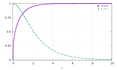
Figure 1: Profiles of $f(r)$ and $\phi(r)$ for the CM monopole.

A less trivial situation arises for $\nu=\pm 1$, hence for the magnetic charge $n=\pm 2$. Eqs.(IV) then admit a smooth solution for which the amplitudes $f,\phi$ interpolate between the following asymptotic values:

$$f=1+{\cal O}(r^{2}),~{}~{}~{}~{}~{}\phi={\cal O}(r^{\delta})~{}~{}~{}~{}~{}~{}\text{for}~{}~{}~{}~{}~{}r\to 0$$ (4.14)

with $\delta=(\sqrt{3}-1)/2$ and

$$f={\cal O}\left(e^{-m_{\mbox{\tiny W}}r}\right),~{}~{}~{}~{}~{}\phi=1+{\cal O}\left(e^{-m_{\mbox{\tiny H}}r}\right)~{}~{}~{}~{}~{}~{}\text{for}~{}~{}~{}~{}~{}r\to\infty.$$ (4.15)

This solution can be obtained numerically, see Fig.1, and its existence was proven in yang2014solitons . At infinity the fields approach those for the magnetic monopole with $n=\pm 2$, while at the origin the non-Abelian fields are regular and their contribution to the energy is finite. However, the U(1) contribution to the energy is infinite. The energy can be represented as $E=E_{0}+E_{1}$ where $E_{1}$ is finite but $E_{0}$ diverges,

$$E_{0} = \frac{2\pi}{g^{\prime 2}}\int_{0}^{\infty}{\frac{dr}{r^{2}}},$$

$$E_{1} = 4\pi\int_{0}^{\infty}dr\left(\frac{1}{g^{2}}\left(\frac{(f^{2}-1)^{2}}{2r^{2}}+f^{\prime 2}\right)+(r\phi^{\prime})^{2}+\frac{r^{2}\beta}{8}(\phi^{2}-1)^{2}+\frac{1}{2}(f\phi)^{2}\right).$$ (4.16)

This solution can be generalized by adding the electric amplitudes $\Omega_{0}$ and $\Theta_{0}$ and solving Eqs.(IV).

IV.3 Oscillating solutions

The only possibility to obtain finite energy solutions is to choose $\nu=0$, in which case the singular at the origin term ${\cal E}_{\nu}$ in (III) vanishes. One should then set $f=0$ and Eqs.(III),(III) reduce to

$$\frac{1}{r^{2}}\,(r^{2}\phi^{\prime})^{\prime}-\ddot{\phi} = \frac{1}{4}\left(\beta(\phi^{2}-1)+\Theta_{1}^{2}-\Theta_{0}^{2}\right)\phi\,,$$

$$\frac{1}{r^{2}}\left(r^{2}(\Omega_{0}^{\prime}-\dot{\Omega}_{1})\right)^{\prime} = \frac{g^{2}}{2}\,\phi^{2}\Theta_{0}\,,~{}~{}~{}~{}~{}\left(\Omega_{0}^{\prime}-\dot{\Omega}_{1}\right)^{\mbox{$\cdot$}}=\frac{g^{2}}{2}\,\phi^{2}\Theta_{1}\,,$$

$$\frac{1}{r^{2}}\left(r^{2}(\Theta_{0}^{\prime}-\dot{\Theta}_{1})\right)^{\prime} = \frac{1}{2}\,\phi^{2}\Theta_{0}\,,~{}~{}~{}~{}~{}~{}\left(\Theta_{0}^{\prime}-\dot{\Theta}_{1}\right)^{\mbox{$\cdot$}}=\frac{1}{2}\,\phi^{2}\Theta_{1}\,.$$ (4.17)

One can show that non-trivial static solutions of these equations have infinite energy. However, there are time-dependent solutions with a finite energy. Solutions of this type were previously studied assuming the sphaleron anstaz (1.2) for the Higgs field, in which case the fields are not spherically symmetric, unless for $\theta_{\mbox{\tiny W}}=0$ Ratra:1987dp ; Farhi:2005rz ; Graham:2006vy ; Graham:2007ds . On the other hand, Eqs.(IV.3) describe spherically symmetric systems for any $\theta_{\mbox{\tiny W}}$.

Let us set the gauge fields to zero, $\Omega_{0}=\Omega_{1}=\Theta_{0}=\Theta_{1}=0$. Rescaling the spacetime coordinates via $t\to 2/\sqrt{\beta}\,t$ and $r\to 2/\sqrt{\beta}\,r$, the remaining Higgs equation reduces to

$$\frac{1}{r^{2}}\,(r^{2}\phi^{\prime})^{\prime}-\ddot{\phi}=(\phi^{2}-1)\phi.$$ (4.18)

This equation has been extensively studied, and it is known that it describes oscillons – oscillating quaziperiodic configurations with a finite energy Copeland:1995fq ; Honda:2001xg ; Fodor:2006zs . Oscillons are well-localized in space during a certain period of time but finally they decay into a pure radiation. However, their lifetime, that is the period when they remain localized, can be very large, depending on the initial values. In principle, their lifetime can be comparable with the age of the universe. We therefore discover that the electroweak theory admits spherically symmetric oscillons, which, to the best of our knowledge, has never been observed before. We shall present separately their detailed analysis as well as more general solutions of (IV.3) GGV .

V SPERICALLY SYMMETRIC PERTURBATIONS

Consider small perturbations around a static and purely magnetic background

$$f(r)\to{f}(r)+\delta f(t,r),~{}~{}~{}\phi(r)\to{\phi}(r)+\delta\phi(t,r),~{}$$ (5.19)

and also

$$\Omega_{0}(t,r) = \delta\Omega_{0}(t,r),~{}~{}~{}~{}\Omega_{1}(t,r)=\delta\Omega_{1}(t,r),~{}~{}$$

$$\Theta_{0}(t,r) = \delta\Theta_{0}(t,r),~{}~{}~{}~{}\Theta_{1}(t,r)=\delta\Theta_{1}(t,r).$$ (5.20)

Injecting this to Eqs.(III)–(III) and linearizing with respect to the perturbations, the linearized equations split into two independent groups containing, respectively, the perturbation described by (5.19) and those in (V).

V.1 Perturbations of the CM monopole

Setting

$$\delta f(t,r)=e^{i\omega t}\,\psi_{1}(r),~{}~{}~{}~{}~{}~{}\delta\phi(t,r)=\frac{1}{gr}\,e^{i\omega t}\,\psi_{2}(r),$$ (5.21)

injecting to (III) and linearizing yields the two-channel eigenvalue problem

$$\left(-\frac{d^{2}}{dr^{2}}+\hat{V}\right)\Psi=\omega^{2}\Psi~{}~{}~{}~{}~{}\text{with}~{}~{}~{}~{}\Psi=\begin{pmatrix}\psi_{1}\\ \psi_{2}\end{pmatrix},$$ (5.22)

where the potential $\hat{V}$ is a symmetric $2\times 2$ matrix with components

$$V_{11} = \frac{g^{2}}{2}\,\phi^{2}+\frac{3f^{2}-1}{r^{2}},~{}~{}~{}~{}~{}V_{22}=\frac{\beta}{4}\,(3\phi^{2}-1)+\frac{f^{2}}{2r^{2}},~{}~{}~{}~{}~{}V_{12}=V_{21}=g\frac{f\phi}{r}\,.$$ (5.23)

Linearizing similarly Eqs.(III),(3.14) with respect to perturbations and setting

$$\delta\Omega_{1}(t,r) = \,\frac{g\,e^{i\omega t}}{f}\,\psi_{1}(r),~{}~{}~{}~{}~{}~{}~{}~{}~{}~{}~{}~{}~{}\delta\Theta_{1}(t,r)=\frac{2\,e^{i\omega t}}{r\phi}\,\psi_{2}(r),$$

$$\delta\Omega_{0}(t,r) = \frac{g\,e^{i\omega t}}{i\omega}\,\frac{1}{f^{2}}\left(f\psi_{1}\right)^{\prime},~{}~{}~{}~{}~{}~{}\delta\Theta_{0}(t,r)=\frac{2\,e^{i\omega t}}{i\omega}\,\frac{1}{r^{2}\phi^{2}}\left(r\phi\,\psi_{2}\right)^{\prime}$$ (5.24)

yields again the eigenvalue problem of the form (5.22) with the following components of the potential matrix

$$V_{11} = \frac{f^{2}+1}{r^{2}}+2\,\frac{f^{\prime 2}}{f^{2}}-\frac{g^{2}\phi^{2}}{2}\,,~{}~{}~{}~{}~{}V_{12}=V_{21}=g\frac{f\phi}{r}\,,$$

$$V_{22} = 2\left(\frac{(r\phi)^{\prime}}{r\phi}\right)^{2}+\frac{\phi^{2}}{2}+\frac{\beta}{4}\,(1-\phi)^{2}-\frac{f^{2}}{2r^{2}}\,.$$ (5.25)

Let us assume $f,\phi$ to be those for the CM monopole. One should study the 2-channel eigenvalue problems (5.22) with the potential given by either (5.23) or by (V.1) to see if there is a negative part of spectra of $\omega^{2}$. As will be shown in Section VIII below, the spectra of $\omega^{2}$ are positive in both cases.

As a result, the CM monopole is stable with respect to fluctuations within the spherically symmetric sector. However, it may be unstable with respect to more general perturbations. For example, since it has the magnetic charge $n=\pm 2$, it could in principle split into two monopoles with $n=\pm 1$ via developing an instability in the axially-symmetric sector. Therefore, one should study the more general perturbations, but this requires a much more involved analysis to be described in the following Sections.

V.2 Perturbations of the Abelian monopole

For the Abelian monopole with $\nu=\pm 1$ and $f=0$, $\phi=1$ the above perturbation equations do not apply because (V.1) contains $f$ in the denominator. In addition, using the function $f=\sqrt{w_{1}^{2}+w_{2}^{2}}$ would make no sense within the linear perturbation theory for small $w_{1}$ and $w_{2}$. We shall describe in Section VIII below how to handle the problem in a gauge-invariant way, but for the time being let us return to the original amplitudes $w_{1},w_{2},a_{0},a_{1},b_{0},b_{1},\xi$. They all vanish (modulo gauge transformations) for the monopole background, hence they are small for small fluctuations, while the Higgs field is $\phi=1+\delta\phi$.

Linearizing Eqs.(APENDIX B: ELECTROWEAK EQUATIONS IN THE SPHERICALLY SYMMETRIC SECTOR)–(APENDIX B: ELECTROWEAK EQUATIONS IN THE SPHERICALLY SYMMETRIC SECTOR), one obtains three decoupled from each other equations

$$w_{1}^{\prime\prime}-\ddot{w}_{1}=\left(\frac{g^{2}}{2}-\frac{1}{r^{2}}\right)w_{1}\,,~{}~{}~{}w_{2}^{\prime\prime}-\ddot{w}_{2}=\left(\frac{g^{2}}{2}-\frac{1}{r^{2}}\right)w_{2}\,,~{}~{}~{}\frac{1}{r^{2}}\left(r^{2}\delta\phi^{\prime}\right)^{\prime}-\delta\ddot{\phi}=\frac{\beta}{2}\,\delta\phi,~{}~{}~{}~{}~{}$$ (5.26)

and five coupled equations

$$\left(r^{2}(a_{0}^{\prime}-\dot{a}_{1})\right)^{\prime}-\frac{g^{2}r^{2}}{2}\left(a_{0}-b_{0}+\dot{\xi}\right)=0\,, ~{}~{}~{}~{}\left(r^{2}(a_{0}^{\prime}-\dot{a}_{1})\right)^{\mbox{$\cdot$}}-\frac{g^{2}r^{2}}{2}\left(a_{1}-b_{1}+\xi^{\prime}\right)=0\,,$$

$$\left(r^{2}(b_{0}^{\prime}-\dot{b}_{1})\right)^{\prime}+\frac{g^{\prime 2}r^{2}}{2}\left(a_{0}-b_{0}+\dot{\xi}\right)=0\,, ~{}~{}~{}\left(r^{2}(b_{0}^{\prime}-\dot{b}_{1})\right)^{\mbox{$\cdot$}}+\frac{g^{\prime 2}r^{2}}{2}\left(a_{1}-b_{1}+\xi^{\prime}\right)=0\,,$$

$$\left(r^{2}(a_{1}-b_{1}+\xi^{\prime})\right)^{\prime} = \left(r^{2}(a_{0}-b_{0}+\dot{\xi})\right)^{\mbox{$\cdot$}}\,.~{}~{}~{}~{}~{}~{}~{}~{}$$ (5.27)

The last equation here can be fulfilled by setting

$$r^{2}(a_{1}-b_{1}+\xi^{\prime})=\dot{\Psi},~{}~{}~{}~{}~{}~{}r^{2}(a_{0}-b_{0}+\dot{\xi})=\Psi^{\prime}\,,$$ (5.28)

which implies that the other four equations in (V.2) can be integrated yielding

$$r^{2}(a_{0}^{\prime}-\dot{a}_{1})=\frac{g^{2}}{2}\,\Psi,~{}~{}~{}~{}~{}~{}~{}r^{2}(b_{0}^{\prime}-\dot{b}_{1})=-\frac{g^{\prime 2}}{2}\,\Psi\,,$$ (5.29)

hence

$$(a_{0}-b_{0})^{\prime}-(a_{1}-b_{1})^{\mbox{$\cdot$}}=\frac{\Psi}{2\,r^{2}}\,.$$ (5.30)

On the other hand, one obtains from (5.28)

$$a_{0}-b_{0}=\frac{\Psi^{\prime}}{r^{2}}-\dot{\xi},~{}~{}~{}~{}~{}~{}~{}a_{1}-b_{1}=\frac{\dot{\Psi}}{r^{2}}-\xi^{\prime},$$ (5.31)

injecting which to (5.30) gives

$$\left(\frac{\Psi^{\prime}}{r^{2}}\right)^{\prime}-\left(\frac{\dot{\Psi}}{r^{2}}\right)^{\mbox{$\cdot$}}=\frac{\Psi}{2\,r^{2}}\,,$$ (5.32)

which reduces upon setting $\Psi=e^{i\omega t}\,r\,\psi(r)$ to

$$\left(-\frac{d^{2}}{dr^{2}}+\frac{2}{r^{2}}+\frac{1}{2}\right)\psi=\omega^{2}\psi.$$ (5.33)

Setting $w_{a}=e^{i\omega t}\psi_{a}(r)$ with $a=1,2$ and $\delta\phi=e^{i\omega t}\psi_{3}(r)/r$ the three decoupled equations in (5.26) reduce to

$$\left(-\frac{d}{dr^{2}}-\frac{1}{r^{2}}+\frac{g^{2}}{2}\right)\psi_{a}=\omega^{2}\psi_{a},~{}~{}~{}~{}a=1,2,$$ (5.34)

and to

$$\left(-\frac{d^{2}}{dr^{2}}+\frac{\beta}{2}\right)\psi_{3}=\omega^{2}\psi_{3}\,.$$ (5.35)

As a result, spherically symmetric perturbations of the Abelian monopole split into four independent channels containing the $Z$-boson described by (5.33), the complex-valued $W$-boson described by two real equations (5.34), and the Higgs boson described by (5.35).

One might think that only one of the two equations (5.34) describing $w_{1}$ and $w_{2}$ should be counted, since the local gauge symmetry $w_{1}\to\tilde{w}_{1}=w_{1}\,\cos\gamma-w_{2}\,\sin\gamma$ and $w_{2}\to\tilde{w}_{2}=w_{1}\,\sin\gamma+w_{2}\,\cos\gamma$ contained in (3.6) can be used to set $\tilde{w}_{2}=0$. However, this would require choosing the gauge parameter $\gamma$ such that $\tan\gamma=-w_{2}/w_{1}$. Since $w_{1}$ and $w_{2}$ oscillate around zero, the derivatives of $\gamma$ would then be unbounded. The gauge transformations of the other amplitudes in (3.6), as for example $a_{0}\to a_{0}+\dot{\gamma}$ and $a_{1}\to a_{1}+\gamma^{\prime}$, would be unbounded too. However, within the linear perturbation theory all amplitudes should be small, hence such gauge transformations are not allowed. Therefore, one cannot gauge away one of the two amplitudes $w_{1}$ and $w_{2}$ and each of them should be counted. This will be independently confirmed by the analysis in Section VIII.

Notice finally that the perturbation potentials in the $Z$ and Higgs channells are positive, hence $\omega^{2}>0$. However, in the W-channel the potential admits infinitely many bound states with negative and arbitrarily large $\omega^{2}$. This issue will be discussed in more detail in Section VIII. As a result, the Abelian monopole with $n=2\nu=\pm 2$ is unstable with respect to fluctuations in the spherically symmetric sector. This conclusion does not apply to monopoles with $\nu\neq\pm 1$ since in that case one has $w_{1}=w_{2}=0$ and the spherically symmetric $W$-perturbation channel is closed.

VI GENERIC PERTURBATIONS

Let us consider small fluctuations around a background configuration $(W^{a}_{\mu},B_{\mu},\Phi)$,

$$W^{a}_{\mu}\rightarrow W^{a}_{\mu}+\delta W^{a}_{\mu},\quad\quad B_{\mu}\rightarrow B_{\mu}+\delta B_{\mu},\quad\quad\Phi\rightarrow\Phi+\delta\Phi.$$ (6.36)

Inserting to (2.8) and linearizing with respect to $\delta W^{a}_{\mu}$, $\delta B_{\mu}$, $\delta\Phi$ gives the perturbation equations

$$\nabla_{\mu}\nabla^{\mu}\delta B_{\nu} -\frac{g^{\prime 2}}{2}\left(\Phi^{\dagger}\left(\delta B_{\nu}+\tau_{a}\delta W^{a}_{\nu}\right)\Phi+2i\left(\delta\Phi^{\dagger}D_{\nu}\Phi-(D_{\nu}\Phi)^{\dagger}\delta\Phi\right)\right)$$

$$=\nabla_{\nu}\left(\nabla_{\mu}\delta B^{\mu}-\frac{ig^{\prime 2}}{2}\left(\delta\Phi^{\dagger}\Phi-\Phi^{\dagger}\delta\Phi\right)\right),$$

$$\mathcal{D}_{\mu}\mathcal{D}^{\mu}\delta W^{a}_{\nu} +2\epsilon_{abc}W^{b}_{\nu\mu}\delta W^{c\mu}-\frac{g^{2}}{2}\left(\Phi^{\dagger}\left(\tau_{a}\delta B_{\nu}+\delta W^{a}_{\nu}\right)\Phi+2i\left(\delta\Phi^{\dagger}\tau_{a}D_{\nu}\Phi-(D_{\nu}\Phi)^{\dagger}\tau_{a}\delta\Phi\right)\right)$$

$$=\mathcal{D}_{\nu}\left(\mathcal{D}_{\mu}\delta W^{a\mu}-\frac{ig^{2}}{2}\left(\delta\Phi^{\dagger}\tau_{a}\Phi-\Phi^{\dagger}\tau_{a}\delta\Phi\right)\right),$$

$$D_{\mu}D^{\mu}\delta\Phi -i\left(\delta B_{\mu}+\tau_{a}\delta W^{a}_{\mu}\right)D^{\mu}\Phi-\frac{\beta}{4}\left(\delta\Phi^{\dagger}\Phi+\Phi^{\dagger}\delta\Phi\right)-\frac{\beta}{4}\left(\Phi^{\dagger}\Phi-1\right)\delta\Phi$$

$$=\frac{i}{2}\left(\nabla_{\mu}\delta B^{\mu}+\tau_{a}\mathcal{D}_{\mu}\delta W^{a}_{\mu}\right)\Phi.{}$$ (6.37)

The gauge symmetry is now expressed by the linearized version of transformations (2.6), that is, Eqs. (6.37) are invariant under the replacement

$$\delta\Phi\rightarrow\delta\Phi+\frac{i}{2}\left(\delta\Theta+\tau_{a}\delta\theta^{a}\right)\Phi,\quad\delta B_{\mu}\rightarrow\delta B_{\mu}+\partial_{\mu}\delta\Theta,\quad\delta W^{a}_{\mu}\rightarrow\delta W^{a}_{\mu}+\mathcal{D}_{\mu}\delta\theta^{a},$$ (6.38)

where $\delta\Theta$, $\delta\theta^{a}$ are functions of $t$, $r$, $\vartheta$, $\varphi$.

VI.1 Separation of variables

Let us assume the background fields to be static, spherically symmetric and purely magnetic. It is described by Eqs.(3.2)–(3.4) where one sets $\Omega_{0}=\Omega_{1}=\Theta_{0}=\Theta_{1}=0$ to eliminate the electric fields and for simplicity sets to zero also the pure gauge functions $\alpha,\xi$, which yields

$$W=f(r)\left[{\rm T}_{2}\,d\vartheta-\nu\,T_{1}\,\sin\vartheta\,d\varphi\right]+{\rm T}_{3}\,\nu\cos\vartheta d\varphi,~{}~{}~{}~{}B=\nu\cos\vartheta\,d\varphi\,,~{}~{}~{}~{}\Phi=\begin{pmatrix}0\\ \phi(r)\end{pmatrix}.~{}~{}~{}~{}~{}~{}$$ (6.39)

The parameter $\nu$ can be integer or half-integer and fulfills $(\nu^{2}-1)f=0$. Injecting this to the perturbation equations (6.37) and assuming the perturbations to depend on $t,r,\vartheta,\varphi$, the first step is to separate the variables. This is a non-trivial task because different component of perturbations have different spin and different isospin, and since spin, isospin and the orbital angular momentum are all coupled, this leads to a rather complex angular dependence.

Fortunately, there is a powerful method to treat similar problems, originally proposed within the context of the Newman-Penrose approach in the General Relativity Newman:1961qr . The method is based on introducing the complex-valued spacetime tetrad $\theta^{\alpha}=\theta^{\alpha}_{~{}\mu}\,dx^{\mu}$ consisting of 1-forms

$$\theta^{0}=dt,\quad\quad\theta^{1}=dr,\quad\quad\theta^{2}=\frac{r}{\sqrt{2}}\,(d\vartheta-i\sin\vartheta d\varphi),\quad\quad\theta^{3}=\left(\theta^{2}\right)^{\ast},$$ (6.40)

whose scalar products determine the tetrad metric $\eta^{\alpha\beta}=(\theta^{\alpha},\theta^{\beta})$ with the only non-vanishing elements $\eta_{00}=-1$, $\eta_{11}=\eta_{23}=\eta_{32}=1$. It is worth noting that $\theta^{2}$ and $\theta^{3}$ are null, $(\theta^{2},\theta^{2})=(\theta^{3},\theta^{3})=0$. In addition, instead of the Lie-algebra basis ${\rm T}_{a}$ used in (3.2) one uses new generators ${\rm L}_{1}={\rm T}_{1}-i{\rm T}_{2}$, ${\rm L}_{2}={\rm T}_{1}+i{\rm T}_{2}$, ${\rm L}_{3}={\rm T}_{3}$. The perturbations are decomposed as

$$\delta B_{\mu}=b_{\alpha}\,\theta_{~{}\mu}^{\alpha},~{}~{}~{}~{}~{}~{}~{}\delta W^{a}_{\mu}{\rm T}_{a}=w^{b}_{\alpha}\,\theta^{\alpha}_{~{}\mu}{\rm L}_{b}\,,$$ (6.41)

and it turns out that the angular dependence of the tetrad projections $b_{\alpha}$ and $w^{b}_{\alpha}$ as well as that of the two Higgs components $\delta\Phi^{A}$ ($A=1,2$) is given in terms of the spin-weighted spherical harmonics ${}_{s}Y_{jm}(\vartheta,\varphi)$ Goldberg:1966uu . Here the indices $j,m$ are the usual orbital and azimuthal quantum numbers, while the spin weight $s$ can be integer or half-integer and encodes information about the spin and isospin of perturbations. One has $j=|s|,|s|+1,\ldots$ and $m=-j,-j+1,\ldots,j$. The functions ${}_{0}Y_{jm}(\vartheta,\varphi)$ coincide with the usual spherical harmonics $Y_{jm}(\vartheta,\varphi)$, while for non-zero and integer values of $s$ they can be generated by the lowering ${\cal L}^{-}$ and raising ${\cal L}^{+}$ operators defined by

$${{\cal L}}^{\mp}{{}_{s}Y}_{jm}\equiv\left(\frac{\partial}{\partial\vartheta}\mp\frac{i}{\sin\vartheta}\,\frac{\partial}{\partial\varphi}\pm s\,\cot\vartheta\right){{}_{s}Y}_{jm}=\pm\sqrt{(j\pm s)(j\mp s+1)}\,{{}_{s\mp 1}}Y_{jm}.$$ (6.42)

Acting on ${}_{s}Y_{jm}$ first with ${\cal L}^{-}$ and then with ${\cal L}^{+}$ yields the differential equation

$$\left(\frac{1}{\sin\vartheta}\frac{\partial}{\partial\vartheta}\sin\vartheta\frac{\partial}{\partial\vartheta}+\frac{1}{\sin^{2}\vartheta}\frac{\partial^{2}}{\partial\varphi^{2}}+2is\,\frac{\cos\vartheta}{\sin^{2}\vartheta}\,\frac{\partial}{\partial\varphi}-\frac{s^{2}}{\sin^{2}\vartheta}+j(j+1)\right){{}_{s}}Y_{jm}=0.$$ (6.43)

The $\varphi$-dependence of the harmonics is ${{}_{s}}Y_{jm}\sim e^{im\varphi}$ hence

$${{}_{s}}Y_{j,m}(\vartheta,\varphi)~{}~{}~{}\text{and}~{}~{}~{}~{}\left({{}_{-s}}Y_{j,m}(\vartheta,\varphi)\right)^{\ast}$$ (6.44)

fulfill the same differential equation. From the practical viewpoint, the analysis can be simplified by noting that the perturbations should not depend on the azimuthal quantum number $m$, while for $m=j$ one has

$${{}_{s}}Y(\vartheta,\varphi)_{j,j}=const.\times(\sin\vartheta)^{j}\left(\tan\frac{\vartheta}{2}\right)^{s}e^{i\,j\varphi}.$$ (6.45)

As a result, to determine the angular dependence of all amplitudes, it suffices to consider the following two solutions of (6.43), ${}_{s}{\Sigma}_{j}(\vartheta)\,e^{+ij\varphi}$ and ${}_{-s}{\Sigma}_{j}(\vartheta)\,e^{-ij\varphi}$, both with the same spin weight $s$, where

$${}_{s}{\Sigma}_{j}(\vartheta)=\left(\sin\vartheta\right)^{j}\left(\tan\frac{\vartheta}{2}\right)^{s}.$$ (6.46)

To separate the variables, we set

$$b_{\alpha}=b^{+}_{\alpha}(r)\,{{}_{s}}{\Sigma}_{j}(\vartheta)\operatorname{e}^{+i(\omega t+j\varphi)}+b^{-}_{\alpha}(r)\,{{}_{-s}}{\Sigma}_{j}(\vartheta)\operatorname{e}^{-i(\omega t+j\varphi)}$$ (6.47)

where $b^{+}_{\alpha}(r)$ and $b^{-}_{\alpha}(r)$ are complex-valued radial functions. Both terms on the right here have the same spin weight $s$ whose value depends on value of the index $\alpha$ and on the winding number $\nu$. Similar expressions are used for $w^{b}_{\alpha}$ and for $\delta\Phi,\delta\Phi^{\dagger}$. The perturbations contain the $``+"$ part proportional to $\operatorname{e}^{+i(\omega t+j\varphi)}$ and the $``-"$ part proportional to $\operatorname{e}^{-i(\omega t+j\varphi)}$. One cannot retain only one of these parts because they are intermixed in the equations which contain both $\delta\Phi$ and $\delta\Phi^{\dagger}$. This doubles the number of the radial amplitudes: for example 4 components of $b_{\alpha}$ in (6.47) contain 8 radial functions $b^{+}_{\alpha}(r)$ and $b^{-}_{\alpha}(r)$. A similar doubling occurs for radial functions in $w^{b}_{\alpha}$ and $\delta\Phi,\delta\Phi^{\dagger}$. As a result, injecting everything to the equations and setting separately to zero the parts of the equations proportional to $\operatorname{e}^{+i(\omega t+j\varphi)}$ and those proportional to $\operatorname{e}^{-i(\omega t+j\varphi)}$ yields 40 differential equations. These equations contain 40 complex functions of $r$ contained in 20 components of $b_{\alpha},w^{b}_{\alpha},\delta\Phi,\delta\Phi^{\dagger}$ and also functions ${}_{\pm s}\Sigma_{j}(\vartheta)$ with the component-dependent value of $s$.

A direct inspection of the equations then reveals that one can adjust the values of the spin weight $s$ for all components such that the $\vartheta$-dependence in all 40 equations factorizes. This yields 40 ordinary differential equations for 40 complex functions of $r$. A further inspection shows that, imposing simple linear relations between the functions of $r$ contained in the “$+$” part and those contained in the “$-$” part reduces twice the number of independent equations. This yields 20 equations for 20 complex functions of $r$. At the end of the day, one imposes the reality conditions: the spacetime components $\delta B_{\mu}$ and $\delta W^{a}_{\mu}$ should be real, while components of $\delta\Phi$ and $\delta\Phi^{\dagger}$ should be mutually complex conjugated. This renders all 20 functions of $r$ real-valued.

Skipping the details, here is the resulting ansatz that provides the complete separation of the angular and temporal variables. Defining ${\Omega}=\omega t+j\varphi$, the 4 tetrad components $b_{\alpha}$ and their spin weights $s$ are given by

$$b_{0} = +2\cos({\Omega})\,{{}_{0}}\Sigma_{j}(\vartheta)\,\frac{S_{0}(r)}{r}\,,\hskip 170.71652pt(s=0)$$

$$b_{1} = -2\sin({\Omega})\,{{}_{0}}\Sigma_{j}(\vartheta)\,\frac{S_{1}(r)}{r}\,,\hskip 170.71652pt(s=0)$$

$$b_{2} = i\,e^{+i{\Omega}}\,{{}_{+1}}{\Sigma}_{j}(\vartheta)\,\frac{S_{2}(r)}{r}-i\,e^{-i{\Omega}}\,{{}_{-1}}{\Sigma}_{j}(\vartheta)\,\frac{S_{3}(r)}{r},\hskip 56.9055pt(s=+1)$$

$$b_{3} = i\,e^{+i{\Omega}}\,{{}_{-1}}{\Sigma}_{j}(\vartheta)\,\frac{S_{3}(r)}{r}-i\,e^{-i{\Omega}}\,{{}_{+1}}{\Sigma}_{j}(\vartheta)\,\frac{S_{2}(r)}{r},\hskip 56.9055pt(s=-1)$$ (6.48)

the tetrad components $w^{1}_{\alpha}$ are

$$w^{1}_{0} = e^{i{\Omega}}\,{{}_{-\nu}}{\Sigma}_{j}(\vartheta)\,\frac{X_{10}(r)}{r}+e^{-i{\Omega}}\,{{}_{+\nu}}{\Sigma}_{j}(\vartheta)\,\frac{X_{20}(r)}{r}\,,\hskip 56.9055pt(s=-\nu)$$

$$w^{1}_{1} = i\,e^{i{\Omega}}\,{{}_{-\nu}}{\Sigma}_{j}(\vartheta)\,\frac{X_{11}(r)}{r}-i\,e^{-i{\Omega}}\,{{}_{+\nu}}{\Sigma}_{j}(\vartheta)\,\frac{X_{21}(r)}{r}\,,\hskip 51.21504pt(s=-\nu),$$

$$w^{1}_{2} = i\,e^{i{\Omega}}\,{{}_{+1-\nu}}{\Sigma}_{j}(\vartheta)\,\frac{X_{12}(r)}{r}-i\,e^{-i{\Omega}}\,{{}_{+\nu-1}}{\Sigma}_{j}(\vartheta)\,\frac{X_{23}(r)}{r}\,,\hskip 22.76228pt(s=1-\nu)$$

$$w^{1}_{3} = i\,e^{i{\Omega}}\,{{}_{-1-\nu}}{\Sigma}_{j}(\vartheta)\,\frac{X_{13}(r)}{r}-i\,e^{-i{\Omega}}\,{{}_{+\nu+1}}{\Sigma}_{j}(\vartheta)\,\frac{X_{22}(r)}{r}\,,\hskip 19.91684pt(s=-1-\nu)$$ (6.49)

the tetrad components $w^{2}_{\alpha}$ are

$$w^{2}_{0} = e^{i{\Omega}}\,{{}_{+\nu}}{\Sigma}_{j}(\vartheta)\,\frac{X_{20}(r)}{r}+e^{-i{\Omega}}\,{{}_{-\nu}}{\Sigma}_{j}(\vartheta)\,\frac{X_{10}(r)}{r}\,,\hskip 68.28644pt(s=\nu)$$

$$w^{2}_{1} = i\,e^{i{\Omega}}\,{{}_{+\nu}}{\Sigma}_{j}(\vartheta)\,\frac{X_{21}(r)}{r}-i\,e^{-i{\Omega}}\,{{}_{-\nu}}{\Sigma}_{j}(\vartheta)\,\frac{X_{11}(r)}{r}\,,\hskip 56.9055pt(s=\nu)$$

$$w^{2}_{2} = i\,e^{i{\Omega}}\,{{}_{+1+\nu}}{\Sigma}_{j}(\vartheta)\,\frac{X_{22}(r)}{r}-i\,e^{-i{\Omega}}\,{{}_{-\nu-1}}{\Sigma}_{j}(\vartheta)\,\frac{X_{13}(r)}{r}\,,\hskip 19.91684pt(s=1+\nu)$$

$$w^{2}_{3} = i\,e^{i{\Omega}}\,{{}_{-1+\nu}}{\Sigma}_{j}(\vartheta)\,\frac{X_{23}(r)}{r}-i\,e^{-i{\Omega}}\,{{}_{-\nu+1}}{\Sigma}_{j}(\vartheta)\,\frac{X_{12}(r)}{r}\,,\hskip 19.91684pt(s=-1+\nu)$$ (6.50)

the tetrad components $w^{3}_{\alpha}$ read

$$w^{3}_{0} = 2\cos({\Omega})\,{{}_{0}}{\Sigma}_{j}(\vartheta)\,\frac{X_{30}(r)}{r}\,,\hskip 176.407pt(s=0)$$

$$w^{3}_{1} = -2\sin({\Omega})\,{{}_{0}}{\Sigma}_{j}(\vartheta)\,\frac{X_{31}(r)}{r}\,,\hskip 170.71652pt(s=0)$$

$$w^{3}_{2} = i\,e^{i{\Omega}}\,{{}_{+1}}{\Sigma}_{j}(\vartheta)\,\frac{X_{32}(r)}{r}-i\,e^{-i{\Omega}}\,{{}_{-1}}{\Sigma}_{j}(\vartheta)\,\frac{X_{33}(r)}{r}\,,\hskip 56.9055pt(s=1)$$

$$w^{3}_{3} = i\,e^{i{\Omega}}\,{{}_{-1}}{\Sigma}_{j}(\vartheta)\,\frac{X_{33}(r)}{r}-i\,e^{-i{\Omega}}\,{{}_{+1}}{\Sigma}_{j}(\vartheta)\,\frac{X_{32}(r)}{r}\,,\hskip 56.9055pt(s=-1)\$$ (6.51)

while the perturbations of the Higgs field are described by

$$\delta\Phi_{1} = e^{i{\Omega}}\,{{}_{-\nu}}{\Sigma}_{j}(\vartheta)\,\frac{H_{1}(r)}{r}+e^{-i{\Omega}}\,{{}_{+\nu}}{\Sigma}_{j}(\vartheta)\,\frac{H_{2}(r)}{r}\,,\hskip 42.67912pt(s=-\nu)$$

$$\delta\Phi_{2} = e^{i{\Omega}}\,{{}_{0}}{\Sigma}_{j}(\vartheta)\,\frac{H_{3}(r)}{r}+e^{-i{\Omega}}\,{{}_{0}}{\Sigma}_{j}(\vartheta)\,\frac{H_{4}(r)}{r}\,.\hskip 56.9055pt(s=0)$$ (6.52)

Here the 20 radial functions $S_{0}(r),S_{1}(r),\ldots,H_{4}(r)$ are all real-valued. Inserting (6.48)–(6.52) into the perturbation equations (6.37), the variables separate yielding 20 ordinary differential equations for the 20 radial functions. These are Eqs.(C.2a)–(C.7d) shown in Appendix C. The variables separate if only the background condition $(\nu^{2}-1)f=0$ is fulfilled. Therefore Eqs.(C.2a)–(C.7d) make sense if only either $\nu=\pm 1$ when $f(r)$ can be arbitrary or if $f(r)=0$ when $\nu$ can be arbitrary.

Notice finally that the above separation ansatz can be extended to arbitrary values of the azimuthal quantum number $m$ via replacing everywhere in (6.48)–(6.52)

$${{}_{s}}\Sigma_{j}(\vartheta)e^{ij\varphi}\to{{}_{s}}Y_{jm}(\vartheta,\varphi)\,,~{}~{}~{}~{}~{}~{}~{}~{}~{}{{}_{-s}}\Sigma_{j}(\vartheta)e^{-ij\varphi}\to\left({{}_{-s}}Y_{jm}(\vartheta,\varphi)\right)^{\ast}\,.$$ (6.53)

VII GAUGE FIXING

The radial equations (C.2a)–(C.7d) admit the gauge symmetry generated by the gauge transformations (6.38) with the gauge parameters $\delta\Theta$ and $\delta\theta^{a}$ chosen as

$$\delta\Theta = \sin(\Omega)\,{{}_{0}}{\Sigma}_{j}(\vartheta)\,\frac{u(r)}{r}\,,~{}~{}~{}~{}~{}\delta\theta^{3}=\sin(\Omega)\,{{}_{0}}{\Sigma}_{j}(\vartheta)\,\frac{u_{3}(r)}{r}\,,$$

$$\delta\theta_{1} = \sin(\Omega)\,\left({{}_{\nu}}{\Sigma}_{j}(\vartheta)\,\frac{u_{1}(r)}{r}+{{}_{-\nu}}{\Sigma}_{j}(\vartheta)\,\frac{u_{2}(r)}{r}\right)\,,$$

$$\delta\theta_{2} = -\cos(\Omega)\,\left({{}_{\nu}}{\Sigma}_{j}(\vartheta)\,\frac{u_{1}(r)}{r}-{{}_{-\nu}}{\Sigma}_{j}(\vartheta)\,\frac{u_{2}(r)}{r}\right)\,.$$ (7.54)

This choice of the gauge parameters is compatible with the considered above separation of variable and generates the following transformations of the radial functions:

$$S_{0}\to S_{0}+\frac{\omega}{2}\,u,~{}~{}~{}~{}~{}S_{1}\to S_{1}-\frac{r}{2}\left(\frac{u}{r}\right)^{\prime},~{}~{}~{}~{}$$

$$S_{2}\to S_{2}+\frac{j\,u}{2\sqrt{2}\,r},~{}~{}~{}~{}~{}S_{3}\to S_{3}-\frac{j\,u}{2\sqrt{2}\,r},$$ (7.55)

$$X_{10}\to X_{10}+\omega\,u_{2},~{}~{}~{}~{}~{}~{}~{}~{}~{}X_{11}\to X_{11}-r\left(\frac{u_{2}}{r}\right)^{\prime},~{}~{}$$

$$X_{12}\to X_{12}+\frac{1}{\sqrt{2}\,r}\left((\nu+j)\,u_{2}-f\,\delta_{0,1-\nu}\,u_{3}\right),~{}~{}$$

$$X_{13}\to X_{13}+\frac{1}{\sqrt{2}\,r}\left((\nu-j)\,u_{2}-f\,\delta_{0,1+\nu}\,u_{3}\right),~{}$$ (7.56)

$$X_{20}\to X_{20}+\omega\,u_{1},~{}~{}~{}~{}~{}~{}X_{21}\to X_{21}-r\left(\frac{u_{1}}{r}\right)^{\prime},~{}~{}$$

$$X_{22}\to X_{22}+\frac{1}{\sqrt{2}\,r}\left((j-\nu)\,u_{1}-f\,\delta_{0,1+\nu}\,u_{3}\right),~{}~{}~{}$$

$$X_{23}\to X_{23}-\frac{1}{\sqrt{2}\,r}\left((j+\nu)\,u_{1}+f\,\delta_{0,1-\nu}\,u_{3}\right),~{}~{}~{}$$ (7.57)

$$X_{30}\to X_{30}+\frac{\omega}{2}\,u_{3},~{}~{}~{}~{}~{}~{}~{}~{}X_{31}\to X_{31}-\frac{r}{2}\left(\frac{u_{3}}{r}\right)^{\prime},~{}$$

$$X_{32}\to X_{32}+\frac{1}{\sqrt{2}\,r}\left(\frac{j}{2}\,u_{3}+f\,\delta_{0,1-\nu}\,u_{1}+f\,\delta_{0,1+\nu}\,u_{2}\right),~{}$$

$$X_{33}\to X_{33}+\frac{1}{\sqrt{2}\,r}\left(-\frac{j}{2}\,u_{3}+f\,\delta_{0,1+\nu}\,u_{1}+f\,\delta_{0,1-\nu}\,u_{2}\right),~{}$$ (7.58)

$$H_{1}\to H_{1}+\phi\,\frac{u_{2}}{2}\,,~{}~{}~{}~{}~{}~{}~{}~{}~{}H_{2}\to H_{2}-\phi\,\frac{u_{1}}{2},~{}~{}$$

$$H_{3}\to H_{3}+\phi\,\frac{u-u_{3}}{4},~{}~{}~{}~{}~{}~{}H_{4}\to H_{4}+\phi\,\frac{u_{3}-u}{4}.$$ (7.59)

A straightforward verification shows that these transformations leave the radial equations (C.2a)–(C.7d) invariant, provided that the background equations for $f(r)$ and $\phi(r)$ are fulfilled. The four arbitrary functions $u(r),u_{1}(r),u_{2}(r),u_{3}(r)$ generating these transformations can be adjusted to impose four gauge conditions. A convenient gauge choice is

$${\cal C}_{1}=0,~{}~{}~{}~{}{\cal C}_{2}=0,~{}~{}~{}~{}{\cal C}_{3}=0,~{}~{}~{}~{}{\cal C}_{4}=0,~{}~{}~{}~{}$$ (7.60)

where ${\cal C}_{A}$ $(A=1,2,3,4)$ are defined by Eqs.(C.1a)–(C.1d) in Appendix C. This gauge choice implies that

$$\nabla_{\mu}\delta B^{\mu}-\frac{ig^{\prime 2}}{2}\left(\delta\Phi^{\dagger}\Phi-\Phi^{\dagger}\delta\Phi\right)=0,~{}~{}~{}~{}~{}~{}\mathcal{D}_{\mu}\delta W^{a\mu}-\frac{ig^{2}}{2}\left(\delta\Phi^{\dagger}\tau_{a}\Phi-\Phi^{\dagger}\tau_{a}\delta\Phi\right)=0,$$ (7.61)

and hence the right hand sides of perturbation equations for $\delta B_{\mu}$ and $\delta W^{a}_{\mu}$ in (6.37) and of the radial equations (C.2a)–(C.7d) vanish. The radial equations then split into two independent groups because the 4 equations (C.2a),(C.4a),(C.5a),(C.6a) will contain only the temporal components of the fields and reduce to a coupled system,

$$\hat{{\cal D}}X_{10}+\frac{2\nu\,j\,f}{r^{2}}\,X_{30}=0\,,~{}~{}~{}~{}~{}~{}\hat{{\cal D}}X_{20}-\frac{2\nu\,j\,f}{r^{2}}\,X_{30}=0\,,~{}~{}~{}~{}~{}~{}\hat{{\cal D}}_{s}\,S_{0}+\frac{g^{\prime 2}\phi^{2}}{2}\,X_{30}=0\,,$$

$$\left(\hat{{\cal D}}-\frac{f^{2}+\nu^{2}}{r^{2}}\right)X_{30}+\frac{\nu\,(j+1)\,f}{r^{2}}\,(X_{10}-X_{20})+\frac{g^{2}\phi^{2}}{2}\,S_{0}=0\,,$$ (7.62)

with $\hat{{\cal D}}$ defined in (C.3). The remaining 16 equations in (C.2a)–(C.7d) will contain only the remaining 16 field components. The 4 constraints ${\cal C}_{A}=0$ can be resolved with respect to the 4 temporal components,

$$X_{10} =\frac{1}{\omega}\left(\frac{\left(rX_{11}\right)^{\prime}}{r}+\frac{j-\nu_{-}}{\sqrt{2}\,r}\,X_{12}-\frac{j+\nu_{+}}{\sqrt{2}\,r}\,X_{13}-\frac{\nu_{-}\,f}{\sqrt{2}\,r}\,X_{32}+\frac{\nu_{+}\,f}{\sqrt{2}\,r}\,X_{33}+g^{2}\phi\,H_{1}\right)\,,$$

$$X_{20} =\frac{1}{\omega}\left(\frac{\left(rX_{21}\right)^{\prime}}{r}+\frac{j+\nu_{+}}{\sqrt{2}\,r}\,X_{22}-\frac{j-\nu_{-}}{\sqrt{2}\,r}\,X_{23}+\frac{\nu_{+}\,f}{\sqrt{2}\,r}\,X_{32}-\frac{\nu_{-}\,f}{\sqrt{2}\,r}\,X_{33}-g^{2}\phi\,H_{2}\right)\,,$$

$$X_{30} =\frac{1}{\omega}\left(\frac{\left(rX_{31}\right)^{\prime}}{r}+\frac{\nu_{-}\,f}{2\sqrt{2}\,r}\,(X_{13}+X_{22})-\frac{\nu_{+}\,f}{2\sqrt{2}\,r}\,(X_{12}+X_{23})\right.$$

$$\hskip 199.16928pt\left.+\frac{j+1}{\sqrt{2}\,r}\,(X_{32}-X_{33})+\frac{g^{2}}{2}\,\phi\,(H_{4}-H_{3})\right)\,,$$

$$S_{0} =\frac{1}{\omega}\left(\frac{\left(rS_{1}\right)^{\prime}}{r}+\frac{j+1}{\sqrt{2}\,r}\,(S_{2}-S_{3})+\frac{g^{\prime 2}}{2}\,\phi\,(H_{3}-H_{4})\right)\,.$$ (7.63)

Injecting this to the 4 equations (VII) and using the background equations yields identities by virtue of the 16 equations for the 16 functions that appear on the right in (7.63). Therefore, the number of independent radial functions reduces to $16=20-4$. This corresponds to the 12 physical degrees of freedom of the fields plus additional 4 gauge degrees of freedom. The additional gauge degrees appear because the gauge conditions ${\cal C}_{A}=0$ do not fix the gauge completely. Specifically, the gauge conditions ${\cal C}_{A}=0$ will be invariant under gauge transformations (7.55)–(7.59) if the parameters $u(r),u_{1}(r),u_{2}(r),u_{3}(r)$ of the latter fulfill equations that have exactly the same structure as Eqs.(VII), up to the replacement

$$X_{10}\to u_{2},~{}~{}~{}~{}X_{20}\to u_{1},~{}~{}~{}~{}X_{30}\to\frac{u_{3}}{2},~{}~{}~{}S_{0}\to\frac{u}{2}.$$ (7.64)

Defining $u_{\pm}=u_{1}\pm u_{2}$, these equations can be represented as one independent equation

$$\hat{{\cal D}}\,u_{+}=0,$$ (7.65)

and three coupled equations

$$\hat{{\cal D}}\,u_{-}-\frac{2\nu\,j\,f}{r^{2}}\,u_{3}=0,~{}~{}~{}~{}~{}~{}\hat{{\cal D}}_{s}\,u+\frac{g^{\prime 2}\phi^{2}}{2}\,u_{3}=0,$$

$$\left(\hat{{\cal D}}-\frac{f^{2}+\nu^{2}}{r^{2}}\right)u_{3}-\frac{2\nu\,(j+1)\,f}{r^{2}}\,u_{-}+\frac{g^{2}\phi^{2}}{2}\,u=0,$$ (7.66)

with $\hat{{\cal D}}$ and $\hat{{\cal D}}_{s}$ defined in (C.3),(APENDIX C: PERTURBATION EQUATIONS AFTER VARIABLE SEPARATION). Solutions of these equations generate gauge transformations which preserve the ${\cal C}_{A}=0$ conditions. One possibility to use this residual symmetry is to impose extra gauge conditions and pass to the temporal gauge by setting $X_{10}=X_{20}=X_{30}=S_{0}=0$. This is possible because the temporal field components in (VII) and the gauge parameters $u,u_{1},u_{2},u_{3}$ satisfy the same equations. In this case the relations (7.63) would become constraints that would further reduce to 12 the number of independent functions. However, explicitly resolving these constraints leads to very complicated expressions. Therefore, instead of using the temporal gauge condition we prefer a different method.

We notice that defining

$$\kappa=\sqrt{\frac{j}{j+1}},~{}~{}~{}~{}~{}~{}~{}~{}~{}\kappa_{\pm}=\sqrt{\frac{j\pm\nu}{j+1\mp\nu}},$$ (7.67)

one can express the 16 functions in terms of 7 amplitudes $Y_{1}(r),\ldots,Y_{7}(r)$ and 9 amplitudes $Z_{1}(r),\ldots,Z_{9}(r)$ as

$$X_{11} = \frac{\kappa}{2}\left[\,Y_{2}(r)+Z_{2}(r)\,\right]\,,~{}~{}~{}~{}~{}~{}~{}~{}~{}X_{12}=\frac{\kappa\,\kappa_{+}}{2}\left[\,Y_{1}(r)+Z_{1}(r)\,\right]\,,$$

$$X_{13} = \frac{\kappa\,\kappa_{-}}{2}\left[\,Y_{4}(r)+Z_{4}(r)\,\right]\,,~{}~{}~{}~{}~{}~{}~{}X_{21}=\frac{\kappa}{2}\left[\,Y_{2}(r)-Z_{2}(r)\,\right]\,,$$

$$X_{22} = \frac{\kappa\,\kappa_{-}}{2}\left[\,-Y_{4}(r)+Z_{4}(r)\,\right]\,,~{}~{}~{}~{}~{}X_{23}=\frac{\kappa\,\kappa_{+}}{2}\left[\,-Y_{1}(r)+Z_{1}(r)\,\right]\,,$$

$$X_{31} = \frac{1}{2}\,\left[\,-g\,Z_{6}(r)+g^{\prime}Z_{8}(r)\,\right]\,,~{}~{}~{}~{}~{}S_{1}=\frac{g^{\prime}}{2g}\,\left[\,g^{\prime}\,Z_{6}(r)+g\,Z_{8}(r)\,\right]\,,$$

$$X_{32} = \left.\left.\frac{\kappa}{2\sqrt{2}}\right(-g\,\left[\,Y_{5}(r)+Z_{7}(r)\,\right]+g^{\prime}\,\left[\,Y_{6}(r)+Z_{9}(r)\,\right]\right)\,,$$

$$X_{33} = \left.\left.\frac{\kappa}{2\sqrt{2}}\right(g\,\left[\,-Y_{5}(r)+Z_{7}(r)\,\right]+g^{\prime}\,\left[\,Y_{6}(r)-Z_{9}(r)\,\right]\right)\,,$$

$$S_{2} = \left.\left.\frac{\kappa\,g^{\prime}}{2\sqrt{2}\,g}\right(g^{\prime}\,\left[\,Y_{5}(r)+Z_{7}(r)\,\right]+g\,\left[\,Y_{6}(r)+Z_{9}(r)\,\right]\right)\,,$$

$$S_{3} = \left.\left.\frac{\kappa\,g^{\prime}}{2\sqrt{2}\,g}\right(g^{\prime}\,\left[\,Y_{5}(r)-Z_{7}(r)\,\right]+g\,\left[\,Y_{6}(r)-Z_{9}(r)\,\right]\right)\,,$$

$$H_{1} = \frac{\kappa}{2\sqrt{2}\,g}\,\left[\,Y_{3}(r)-Z_{3}(r)\,\right]\,,~{}~{}~{}~{}~{}~{}~{}H_{2}=-\frac{\kappa}{2\sqrt{2}\,g}\,\left[\,Y_{3}(r)+Z_{3}(r)\,\right]\,,~{}$$

$$H_{3} = \frac{1}{2\sqrt{2}\,g}\,\left[\,Y_{7}(r)-Z_{5}(r)\,\right]\,,~{}~{}~{}~{}~{}~{}~{}H_{4}=\frac{1}{2\sqrt{2}\,g}\,\left[\,Y_{7}(r)+Z_{5}(r)\,\right]\,.$$ (7.68)

Injecting this to the radial equations (C.2a)–(C.7d), where one should set ${\cal C}_{A}=0$ and omit the 4 equations for the temporal components, the 7 equations for $Y_{1}(r),\ldots,Y_{7}(r)$ decouple from the 9 equations for $Z_{1}(r),\ldots,Z_{9}(r)$. The reason for this is the difference in their behaviour under the parity reflection. To see this, one should restore the full dependence on the spacetime coordinates. For example, the perturbations of the U(1) field are

$$\delta B_{\mu}dx^{\mu}=b_{\alpha}\,\theta^{\alpha}_{~{}\mu}dx^{\mu}=b_{0}\,dt+b_{1}\,dr+\frac{r\,b_{2}}{\sqrt{2}}\,(d\vartheta-i\sin\vartheta\ d\varphi)+\frac{r\,b_{3}}{\sqrt{2}}\,(d\vartheta+i\sin\vartheta\ d\varphi),~{}~{}~{}~{}~{}~{}$$ (7.69)

where $b_{\alpha}$ are determined by (6.48) in terms of $t,r,\vartheta,\varphi$ with $S_{\alpha}(r)$ expressed in terms of $Y_{A}(r)$ and $Z_{B}(r)$ by (7.68) (notice that $b_{0},b_{1}\in\mathbb{R}$ while $b_{3}=(b_{2})^{\ast}$). It turns out that the angle-dependent coefficients in front of the $Y_{A}(r)$ amplitudes and those in front of the $Z_{B}(r)$ amplitudes behave differently under the parity reflection

$$\vartheta\to\pi-\vartheta,~{}~{}~{}~{}~{}~{}\varphi\to\pi+\varphi.$$ (7.70)

If the coefficients in front of the $Y$-amplitudes stay invariant under parity, then those in front of the $Z$-amplitudes change sign, or the other way round, depending on values of $j,\nu$. This explains the separation of the $Y$-equations from the $Z$-equations.

Introducing the 7-component vector $\Psi_{Y}=[Y_{1}(r),\ldots,Y_{7}(r)]^{\rm tr}$ and the 9-component vector $\Psi_{Z}=[Z_{1}(r),\ldots,Z_{9}(r)]^{\rm tr}$, the 16 perturbation equations assume the form of two independent Schroedinger-type systems

$$\left(-\frac{d^{2}}{dr^{2}}+\hat{U}\right)\Psi_{Y}=\omega^{2}\Psi_{Y}\,,~{}~{}~{}~{}~{}\left(-\frac{d^{2}}{dr^{2}}+\hat{V}\right)\Psi_{Z}=\omega^{2}\Psi_{Z}\,,~{}~{}~{}~{}~{}$$ (7.71)

where $\hat{U}$ and $\hat{V}$ are symmetric matrices whose components are shown in Appendix D. In the $r\to\infty$ limit, where $\phi\to 1$ and $f\to 0$, these potentials reduce to

$$\hat{U} = {\rm diag}\left(m_{\mbox{\tiny W}}^{2},m_{\mbox{\tiny W}}^{2},m_{\mbox{\tiny W}}^{2},m_{\mbox{\tiny W}}^{2},m_{\mbox{\tiny Z}}^{2},0,m_{\mbox{\tiny H}}^{2}\right),$$

$$\hat{V} = {\rm diag}\left(m_{\mbox{\tiny W}}^{2},m_{\mbox{\tiny W}}^{2},m_{\mbox{\tiny W}}^{2},m_{\mbox{\tiny W}}^{2},m_{\mbox{\tiny Z}}^{2},m_{\mbox{\tiny Z}}^{2},m_{\mbox{\tiny Z}}^{2},0,0\right),$$ (7.72)

with the field masses given by (2.11). One can see that the $Y$-sector contains four polarization states of the W-boson, one of which is a gauge mode, a $Z$-boson polarization, a photon polarization, and the Higgs mode. The $Y$-sector contains four polarization states of the W-boson one of which is a gauge mode, three $Z$-boson polarizations two of which are gauge modes, and two photon polarizations one of which is a gauge mode.

The gauge modes can be excluded, which can be nicely illustrated for the $Y$-amplitudes. These amplitudes are gauge-dependent, but their transformations under the residual gauge symmetry depend only on the $u_{+}$ gauge amplitude subject to (7.65),

$$Y_{1} \to Y_{1}+\frac{(j+\nu)\,u_{+}}{\sqrt{2}\,\kappa\kappa_{+}\,r}\,,~{}~{}~{}~{}~{}Y_{2}\to Y_{2}-\frac{r}{\kappa}\left(\frac{u_{+}}{r}\right)^{\prime}\,,~{}~{}~{}~{}~{}Y_{3}\to Y_{3}+\frac{g\,\phi\,u_{+}}{\sqrt{2}\,\kappa}\,,~{}~{}~{}~{}$$ (7.73)

$$Y_{4} \to Y_{4}-\frac{(j-\nu)\,u_{+}}{\sqrt{2}\,\kappa\kappa_{-}\,r}\,,~{}~{}~{}~{}~{}~{}Y_{5}\to Y_{5}-\frac{g\,f}{\kappa\,r}\,u_{+}\,,~{}~{}~{}~{}~{}~{}Y_{6}\to Y_{6}+\frac{g^{\prime}\,f}{\kappa\,r}\,u_{+}\,,~{}~{}~{}~{}Y_{7}\to Y_{7}.$$

This implies that the following 6 “calligraphic” combinations are gauge-invariant,

$${\cal Y}_{1} = Y_{1}+\sqrt{\frac{(j+\nu)(j+1-\nu)}{(j-\nu)(j+1+\nu)}}\,Y_{4}\,,~{}~{}~{}~{}~{}~{}{\cal Y}_{2}=Y_{2}-\frac{\sqrt{2}\,r\,Y_{4}^{\prime}}{\sqrt{(j-\nu)(j+1+\nu)}}\,,~{}~{}~{}~{}~{}$$

$${\cal Y}_{3} = Y_{3}+\frac{g\,r\,\phi\,Y_{4}}{\sqrt{(j-\nu)(j+1+\nu)}}\,,~{}~{}~{}~{}~{}~{}~{}~{}~{}{\cal Y}_{5}=Y_{5}-\frac{\sqrt{2}\,g\,f\,Y_{4}}{\sqrt{(j-\nu)(j+1+\nu)}}\,\,,~{}~{}~{}$$

$${\cal Y}_{6} = Y_{6}+\frac{\sqrt{2}\,g^{\prime}\,f\,Y_{4}}{\sqrt{(j-\nu)(j+1+\nu)}}\,\,,~{}~{}~{}~{}{\cal Y}_{4}=Y_{7}\,.$$ (7.74)

Injecting this to the equations (7.71) reveals that these 6 gauge invariant amplitudes fulfill a closed system of 6 equations. The remaining gauge-dependent amplitude $Y_{4}$ filfills (for $\nu=1$) the inhomogeneous equation

$$\hat{{\cal D}}\,(r\,Y_{4})=\left.\left.\frac{\sqrt{2(j-1)(j+2)}}{r}\,\right(f\left(\,g\,{\cal Y}_{5}-g^{\prime}\,{\cal Y}_{6}\,\right)-{\cal Y}_{2}\right).$$ (7.75)

If there are two solutions of this equation which differ from each other by a gauge transformation, $Y_{4}$ and $\tilde{Y}_{4}$, then their difference fulfills the homogeneous equation

$$\hat{{\cal D}}\,(r\,(Y_{4}-\tilde{Y}_{4}))=0,$$ (7.76)

which is compatible with the fact that $r(Y_{4}-\tilde{Y}_{4})\propto u_{+}$ where $\hat{{\cal D}}\,u_{+}=0$.

In the $Z$-sector the residual gauge symmetry is generated by three functions $u_{-},u,u_{3}$ subject to (VII). Defining $v_{\pm}=u\pm u_{3}$ one has

$$Z_{1} \to Z_{1}+\frac{f\,\delta_{0,1-\nu}\,(v_{-}-v_{+})-(j+\nu)\,u_{-}}{\sqrt{2}\,\kappa\kappa_{+}\,r}\,,~{}~{}~{}~{}~{}Z_{2}\to Z_{2}+\frac{r}{\kappa}\left(\frac{u_{-}}{r}\right)^{\prime}\,,~{}~{}~{}~{}Z_{3}\to Z_{3}+\frac{g\,\phi\,u_{-}}{\sqrt{2}\,\kappa}\,,~{}~{}~{}$$

$$Z_{4} \to Z_{4}+\frac{f\,\delta_{0,1+\nu}\,(v_{-}-v_{+})+(j-\nu)\,u_{-}}{\sqrt{2}\,\kappa\kappa_{-}\,r}\,,~{}~{}~{}Z_{5}\to Z_{5}-\frac{g\,\phi\,v_{-}}{\sqrt{2}}\,,~{}~{}~{}~{}~{}~{}Z_{6}\to Z_{6}-g\,r\left(\frac{v_{-}}{r}\right)^{\prime}\,,~{}~{}~{}$$

$$Z_{7} \to Z_{7}+g\,\frac{f\,(\delta_{0,1+\nu}-\delta_{0,1-\nu})\,u_{-}+j\,v_{-}}{\kappa\,r}\,,~{}~{}~{}~{}Z_{8}\to Z_{8}-\frac{g^{2}-g^{\prime 2}}{2g^{\prime}}\,r\left(\frac{v_{-}}{r}\right)^{\prime}-\frac{r}{2g^{\prime}}\left(\frac{v_{+}}{r}\right)^{\prime}\,,$$

$$Z_{9} \to Z_{9}-\frac{g^{\prime}\,f}{\kappa\,r}\,(\delta_{0,1+\nu}-\delta_{0,1-\nu})u_{-}+\frac{j}{2g^{\prime}\kappa}\,((g^{2}-g^{\prime 2})\,v_{-}+v_{+}).$$ (7.77)

Using these expressions one can build 6 gauge invariant amplitudes. It turns out, however, that instead of expressing everything in terms of gauge invariant variables, it is sometimes easier to work with equations (7.71) containing gauge degrees of freedom

VIII STABILITY ANALYSIS

We are now ready to carry out the stability analysis of the monopole solutions. For this one should study the Schroedinger problems (7.71) to see if they admit bound state solutions with $\omega^{2}<0$. Such negative modes are most likely to appear in sectors with lower angular momentum $j$, therefore one should analyze first of all the sectors with $j=0,1$.

In order to consider these sectors one makes use of the following important fact: the spin-weighted harmonics ${{}_{s}}Y_{jm}(\vartheta,\varphi)$ separating the angular variables vanish if $j<|s|$. Physically this corresponds to the fact that modes with angular momentum less than spin are non-dynamical. It can also be seen that the angular functions in (6.45),(6.46) are defined only for $j\geq|s|$ since for $j<|s|$ they would be unbounded.

Therefore, for low values of $j$ all field amplitudes whose spin weight $s$ is too large should be set to zero. Remarkably, this eliminates precisely those amplitudes whose coefficients in the equations become undefined for small $j$ because they contain in the denominators $\kappa=\sqrt{j/(j+1)}$ and $\kappa_{\pm}=\sqrt{(j\pm\nu)/(j+1\mp\nu)}$. Let us see how this works.

VIII.1 $j=0$ sector

The spin weights $s$ of all field amplitudes are shown in (6.48)-(6.52). If $j=0$ then only amplitudes with $s=0$ are allowed. For example, one can see in Eq.(6.48) that $b_{0}$ and $b_{1}$ are allowed, hence the radial amplitudes $S_{0}(r)$ and $S_{1}(r)$ should be kept, but $b_{2}$ and $b_{3}$ should vanish because ${{}_{\pm 1}}\Sigma_{0}=0$ hence one should set $S_{2}=S_{3}=0$. The other non-vanishing amplitudes are $X_{30},X_{31},H_{3},H_{4}$. In addition, one takes into account amplitudes $X_{12}$ and $X_{23}$ if $\nu=1$ since they have spin weights $s=\pm(1-\nu)=0$, whereas for $\nu=-1$ one should keep $X_{22},X_{13}$. Using the definitions of the $Y$ and $Z$ amplitudes in (7.68), we see that the non-vanishing amplitudes are $Y_{7},Z_{5},Z_{6},Z_{8}$ and also $Y_{1},Z_{1}$ if $\nu=1$ (or $Y_{4},Z_{4}$ if $\nu=-1$). All other amplitudes in Eqs.(7.71) should be set to zero.

VIII.1.1 $Y$-sector

The equations (7.71) in the $Y$-sector then reduce for $\nu=1$ to

$$\left(-\frac{d^{2}}{dr^{2}}-\omega^{2}+\frac{3f^{2}-1}{r^{2}}+\frac{g^{2}\phi^{2}}{2}\right)Y_{1}=\frac{gf\,\phi}{r}\,Y_{7}\,,$$

$$\left(-\frac{d^{2}}{dr^{2}}-\omega^{2}+\frac{f^{2}}{2r^{2}}+\frac{\beta}{4}\,(3\phi^{2}-1)\right)Y_{7}=\frac{gf\,\phi}{r}\,Y_{1}\,.$$ (8.78)

Same equations up to $Y_{1}\to Y_{4}$ are obtained for $\nu=-1$. This agrees with the equations previously obtained in (5.22),(5.23) (replacing $Y_{1}\to\psi_{1}$ and $Y_{7}\to-\psi_{2}$). These equations are gauge-invariant since the residual gauge transformations (7.73) in the $Y$-sector are generated by $u_{+}=u_{1}+u_{2}$, however, as seen in (VII), the $u_{1}$ and $u_{2}$ gauge amplitudes have spin weights $s=\pm 1$ and hence vanish for $j=0$. Therefore, there is no residual gauge freedom in this case. For $\nu\neq\pm 1$ one sets $f=0$, $\phi=1$ and $Y_{1}=0$ (also $Y_{4}=0$) and obtains a single equation

$$\left(-\frac{d^{2}}{dr^{2}}+\frac{\beta}{2}\,\right)Y_{7}=\omega^{2}\,Y_{7}\,.$$ (8.79)

Eqs.(VIII.1.1),(8.79) should be studied to see if there are bounded solutions with $\omega^{2}<0$ which would correspond to unstable modes. With the latter equation the situation is simple because it describes a free Higgs mode with $\omega^{2}\geq\beta/2=m_{\mbox{\tiny H}}^{2}$. Therefore, all Abelian monopoles with $\nu\neq\pm 1$ are stable in this sector.

Consider now Eqs.(VIII.1.1) for $\nu=\pm 1$, first in the case when the background is Abelian, $f=0$, $\phi=1$. Then the two equations in (VIII.1.1) decouple from each other. The second one reduces to (8.79) and is precisely the same as Eq.(5.35) derived above. The first equation in (VIII.1.1) becomes the same as one of the two equations in (5.34),

$$\left(-\frac{d^{2}}{dr^{2}}-\frac{1}{r^{2}}+\frac{g^{2}}{2}\right)Y_{1}=\omega^{2}Y_{1}\,.$$ (8.80)

This provides a classical example of an equation admitting infinitely many bound states. Indeed, for $\omega=0$ the solution in the $r\ll 1$ region where one can neglect the $g^{2}/2$ term reads

$$Y_{1}={\cal A}\,\sqrt{r}\,\cos\left(\frac{\sqrt{3}}{2}\,\ln\frac{r}{r_{0}}\right),$$ (8.81)

where ${\cal A},r_{0}$ are integration constants. This solution oscillates infinitely many times as $r\to 0$. According to the well-known Jacobi criterion gelfand2000calculus , since the zero-energy solution oscillates, there are infinitely many bound states with $\omega^{2}<0$. As a result, the $\nu=1$ Abelian monopole in unstable in this sector and the same is true for $\nu=-1$ when one obtains the same equation up to $Y_{1}\to Y_{4}$.

Summarizing, we have recovered in (8.79), (8.80) two of the four equations (5.33)–(5.35) previously obtained in the Abelian case.

Let us now return Eqs.(VIII.1.1) and consider the non-Abelian CM background with $f\neq 0$, $\phi\neq 1$. In this case one can apply the generalization of the Jacobi criterion for multi-channel systems gelfand2000calculus . Setting again $\omega=0$, one can check that in the $r\to 0$ limit, where $f\to 1$ and $\phi\to 0$, the regular at the origin solutions of Eqs.(VIII.1.1) comprise a two-parameter set labeled by two integration constants $C_{1}$ and $C_{2}$,

$$Y_{1}=C_{1}\times(r^{2}+\ldots),~{}~{}~{}~{}~{}Y_{7}=C_{2}\times\left(r^{\frac{1+\sqrt{3}}{2}}+\ldots\right),$$ (8.82)

where the dots denote subleading terms. This determines two independent solutions of the equations: $\left(Y_{1}^{(1)},Y_{7}^{(1)}\right)$ obtained for $(C_{1},C_{2})=(1,0)$, and $\left(Y_{1}^{(2)},Y_{7}^{(2)}\right)$ obtained for $(C_{1},C_{2})=(0,1)$. Integrating the equations numerically then allows one to compute the Jacobi determinant

$$\Delta(r)=\left|\begin{matrix}Y_{1}^{(1)}(r)&~{}Y_{7}^{(1)}(r)\\ Y_{1}^{(2)}(r)&~{}Y_{7}^{(2)}(r)\end{matrix}\right|,$$ (8.83)

and if $\Delta(r)$ crosses zero for $r>0$, then there are bound states with $\omega^{2}<0$. However, as seen in Fig.2, $\Delta(r)$ never vanishes, hence the CM monopole is stable in this sector.

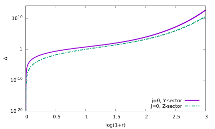
Figure 2: The Jacobi determinant for the CM monopole perturbations in the $Y,Z$ sectors with $j=0$.

VIII.1.2 $Z$-sector

Setting again $\nu=1$, the $Z$-equations (7.71) reduce for $j=0$ to a 4-channel system for the non-vanishing amplitudes $Z_{1},Z_{5},Z_{6},Z_{8}$. This time there is a non-trivial residual gauge symmetry (VII) generated by the gauge parameters $v_{\pm}=u\pm u_{3}$ which have spin weignt $s=0$ and do not vanish for $j=0$. Using the fact that $\kappa\kappa_{+}=1$ for $\nu=1$, the gauge transformations (VII) reduce to

$$Z_{1} \to Z_{1}+\frac{f}{\sqrt{2}r}\,(v_{-}-v_{+})\,,~{}~{}~{}~{}~{}~{}Z_{5}\to Z_{5}-\frac{g\phi}{\sqrt{2}}\,v_{-}\,,$$

$$Z_{6} \to Z_{6}-g\,r\left(\frac{v_{-}}{r}\right)^{\prime}\,,~{}~{}~{}~{}Z_{8}\to Z_{8}+\frac{r}{2g^{\prime}}\left(\frac{v_{-}-v_{+}}{r}\right)^{\prime}-\frac{g^{2}}{g^{\prime}}\,r\left(\frac{v_{-}}{r}\right)^{\prime}\,,$$ (8.84)

and this implies that the following two “calligraphic” combinations

$${\cal Z}_{1}=Z_{8}-\frac{g}{g^{\prime}}\,Z_{6}-\frac{r}{\sqrt{2}\,g^{\prime}}\left(\frac{Z_{1}}{f}\right)^{\prime}\,,~{}~{}~{}~{}~{}~{}~{}~{}{\cal Z}_{2}=Z_{6}-\sqrt{2}\,r\,\left(\frac{Z_{5}}{r\phi}\right)^{\prime}\,,~{}~{}~{}~{}$$ (8.85)

are gauge invariant. Using Eqs.(7.71) one finds that equations for ${\cal Z}_{1}$ and ${\cal Z}_{2}$ decouple from the rest. Setting

$${\cal Z}_{1}=\frac{r\,\psi_{1}}{2g^{\prime}f},~{}~{}~{}~{}~{}~{}~{}{\cal Z}_{2}=-\frac{\psi_{2}}{\phi},~{}~{}~{}~{}~{}$$ (8.86)

the two decoupled gauge-invariant equations read

$$\left(-\frac{d^{2}}{dr^{2}}-\omega^{2}+\frac{f^{2}+1}{r^{2}}+\frac{2f^{\prime 2}}{f^{2}}-\frac{g^{2}\phi^{2}}{2}\right)\psi_{1}+\frac{g\phi\,f}{r}\,\psi_{2} = 0,$$

$$\left(-\frac{d^{2}}{dr^{2}}-\omega^{2}+2\left(\frac{(r\phi)^{\prime}}{r\phi}\right)^{2}+\frac{\phi^{2}}{2}+\frac{\beta}{4}\,(1-\phi)^{2}-\frac{f^{2}}{2r^{2}}\right)\psi_{2}+\frac{g\phi\,f}{r}\,\psi_{1} = 0.$$ (8.87)

This agrees with Eqs.(V.1) derived above. Assuming $f,\phi$ to correspond to the CM background, we integrate these equations to obtain the determinant $\Delta(r)$ constructed from two linearly independent and regular at the origin solutions similar to (8.83). As seen in Fig.2, the determinant is positive, hence the CM monopole is stable in this perturbation sector as well.

The Abelian case where $f=0$ and $\phi=1$ should be considered separately. The gauge transformations (VIII.1.2) imply that the gauge-invariant amplitudes in this case are

$${\cal Z}_{1}=Z_{1},~{}~{}~{}~{}~{}~{}~{}~{}~{}{\cal Z}_{2}=Z_{6}-\sqrt{2}\,r\,\left(\frac{Z_{5}}{r}\right)^{\prime}\,,~{}~{}~{}~{}$$ (8.88)

and these fulfill equations

$$\left(-\frac{d^{2}}{dr^{2}}-\frac{1}{r^{2}}+\frac{g^{2}}{2}\right){\cal Z}_{1}=\omega^{2}{\cal Z}_{1}\,,~{}~{}~{}~{}~{}\left(-\frac{d^{2}}{dr^{2}}+\frac{2}{r^{2}}+\frac{1}{2}\right){\cal Z}_{2}=\omega^{2}{\cal Z}_{2}\,.~{}~{}~{}~{}~{}$$ (8.89)

These are precisely the second of the $W$-equations (5.34) and the $Z$-equation (5.33). Together with (8.79),(8.80), this reproduces all four equations (5.33)–(5.35) previously obtained in the Abelian case. The spectrum in the ${\cal Z}_{2}$-channel is positive but the ${\cal Z}_{1}$-equation admits infinitely many bound states.

The above discussion corresponds to $\nu=1$ but for $\nu=-1$ one obtains the same equations, up to the replacement $Z_{1}\to Z_{4}$. Let us now consider Abelian backgrounds with $f=0$, $\phi=1$ and for $\nu\neq\pm 1$. In this case one should set $Z_{1}=0$ since its spin weight $s=\nu-1\neq 0$, hence there remains only the ${\cal Z}_{2}$ amplitude defined in (8.88). It fulfills the same equation as in (8.89) so that there are no negative modes in this case.

Summarizing, the $\nu=\pm 1$ Abelian monopoles show infinitely many instabilities in the $j=0$ sector while the non-Abelian CM monopole and all Abelian monopoles with $\nu\neq\pm 1$ are stable in this sector.

$k$	$~{}~{}~{}1$	$~{}~{}~{}2$	$~{}~{}~{}3$	$~{}~{}~{}~{}~{}4$	$~{}~{}~{}5$	$~{}~{}~{}6$	$~{}~{}~{}7$	$~{}~{}~{}8$	$~{}~{}~{}9$
$s$ for $Y_{k}:~{}$	$~{}1-\nu$	$~{}-\nu$	$~{}-\nu$	$~{}\pm(1+\nu)$	$~{}~{}~{}1$	$~{}~{}~{}1$	$~{}~{}~{}0$
$s$ for $Z_{k}:~{}$	$~{}1-\nu$	$~{}-\nu$	$~{}-\nu$	$~{}\pm(1+\nu)$	$~{}~{}~{}0$	$~{}~{}~{}0$	$~{}~{}\pm 1$	$~{}~{}~{}0$	$~{}~{}\pm 1$

Table 1: Values of the spin weight $s$ for $Y_{k}$ and $Z_{k}$.

VIII.2 $j=1$ sector

Table I shows spin weights $s$ for amplitudes $Y_{k}$ ($k=1,\ldots,7$) and $Z_{k}$ ($k=1,\ldots,9$). In some cases $s$ is defined only up to sign, as for example $Y_{4}=\kappa\kappa_{-}(X_{13}-X_{22})$ where $X_{13}$ has spin wight $-1-\nu$ and $X_{22}$ has spin wight $1+\nu$. However, only the absolute value $|s|$ is important in what follows.

Let us set $\nu=1$. Then for $Y_{4}$ and $Z_{4}$ one has $|s|=2$ hence these amplitudes should be set to zero if $j=1$. The perturbation equations (7.71) then become

$$-Y_{k}^{\prime\prime}+\sum_{m=1}^{7}U_{km}Y_{m}=\omega^{2}Y_{k}\,,~{}~{}~{}~{}~{}~{}-Z_{k}^{\prime\prime}+\sum_{m=1}^{9}V_{km}Z_{m}=\omega^{2}Z_{k}\,,~{}~{}~{}~{}~{}~{}~{}k,m\neq 4\,,$$ (8.90)

where $U_{km}$ and $V_{km}$ are defined by the expressions shown in Appendix D and restricted to $\nu=j=1$. There are 6 and 8 equations, respectively, in the $Y$ and $Z$ sectors. These equations admit residual gauge symmetry expressed by (7.73) and (VII). One can pass to gauge-invariant amplitudes similarly to what was done above, and then both the $Y$ and $Z$ sectors will contain only 5 equations for 5 gauge-invariant amplitudes. However, to check the stability of the CM background is actually easier by using Eqs.(8.90). These equations describe both physical modes and gauge modes and if they do not show instabilities then the physical modes are all stable.

We apply the Jacobi criterion to (8.90). Let us illustrate the procedure within the $Y$-channel containing 6 equations. To apply the criterion, we set $\omega=0$ and look for 6 independent solutions $Y_{k}^{(a)}$ ($a=1,\ldots 6$) that are regular at the origin. The equations imply that near $r=0$ all solutions should have the structure $Y_{k}(r)=c_{k}\,r^{\alpha}(1+\ldots)$ where the 6 constants $c_{k}$ should fulfill a system of linear homogeneous algebraic equations. Its determinant vanishes for 12 values of $\alpha$ among which 6 are strictly positive. For example, if $g^{2}=3/4$, which is close to $\cos^{2}\theta_{\mbox{\tiny W}}=0.77$, then one finds $\alpha=1,2,3,3,(1+\sqrt{3})/2,(1+\sqrt{15})/2$. This gives rise to 6 regular at the origin solutions, and extending them numerically allows one to compute the Jacobi determinant

$$\Delta(r)=\left|Y_{k}^{(a)}(r)\right|~{}~{}~{}~{}~{}~{}\text{where}~{}~{}~{}a=1,\ldots 6,~{}~{}k=1,2,3,5,6,7.$$ (8.91)

A similar procedure is used in the $Z$-sector. As seen in Fig.3, the Jacobi determinant is positive both in the $Y$ and $Z$ sectors, hence the CM monopole is stable with respect to $j=1$ perturbations. This is an important conclusion since, contrary to what one may expect, this $n=2$ monopole is stable under dipole deformations and does not split into two $n=1$ monopoles.

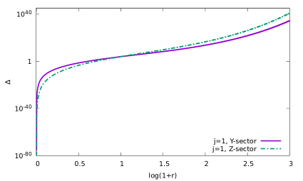
Figure 3: The Jacobi determinant for the CM monopole perturbations in the $Y$,$Z$ sectors with $j=1$.

There remains to study the stability of the Abelian monopoles with $f=0$, $\phi=1$. For $\nu=1$ the equations are provided by (8.90) and it turns out that this Abelian monopole is also stable under dipole deformations, although it is unstable in the $j=0$ sector. For $\nu>2$ one should return to the generic equations (7.71). For $\nu=2$, as seen in Table I, the amplitudes $Y_{2},Y_{3},Y_{4},Z_{2},Z_{3},Z_{4}$ should be set to zero if $j=1$ since their spin weight is too large. All equations then decouple from each other and show no instabilities, apart from the $Y_{1}$ and $Z_{1}$ channels where one finds the equation with infinitely many bound states,

$$\left(-\frac{d^{2}}{dr^{2}}-\frac{2}{r^{2}}+\frac{g^{2}}{2}\right)Y_{1}=\omega^{2}Y_{1}\,,$$ (8.92)

and exactly the same equation for $Z_{1}$. Therefore, the $\nu=2$ monopole is unstable. The same conclusion applies for $\nu=-2$ (one sets $Y_{1}=Y_{2}=Y_{3}=0$, $Z_{1}=Z_{2}=Z_{3}=0$ in this case). No instabilities in the $j=1$ sector are found for $|\nu|>2$.

Summarizing, the non-Abelian CM monopole and all Abelian monopoles with an integer $\nu$ are stable with respect to dipole deformations, apart from the $\nu=\pm 2$ Abelian monopole which shows infinitely many negative modes in the $j=1$ perturbation sector.

VIII.3 Higher values of $j$

If $j\geq 2$ and $\nu=1$ then, as seen in Table I, all amplitudes $Y_{k}$, $Z_{k}$ have spin weights $|s|\leq j$ and hence none of them vanish, so that one should consider the general equations (7.71). Appliyng the Jacobi criterion, we find that they do not admit negative modes for $j=2,3$ (see Fig.4). One could repeat the procedure also for higher values of $j$, but since the centrifugal barrier grows with growing $j$, the existence of negative modes becomes implausible. Therefore, since the CM monopole has no negative modes for $j=0,1,2,3$, this strongly indicates that it is stable with respect to all perturbations.

For the Abelian monopoles the conclusion is different. We already know that the $\nu=1$ monopole is unstable in the $j=0$ sector whereas the $\nu=2$ monopole is unstable in the $j=1$ sector. It turns out that for any given $|\nu|>2$ the corresponding monopole is unstable in the sector with $j=|\nu-1|$ and is stable with respect to all other perturbations. The instability is due to the particular term in the potentials $\hat{U}$ and $\hat{V}$ (see Appendix D),

$$\frac{j(j+1)-\nu^{2}}{r^{2}}\,.$$ (8.93)

The magnetic charge makes the negative contribution to this term, which is the well-known effect for monopoles Coleman:1982cx . If this negative contribution overcomes the positive centrifugal term, then the potential becomes attractive, which produces the instability. For most channels this does not happen since $j$ should be larger than the spin weight determined by $\nu$. However, if $|\nu|>1$ and $j=|\nu|-1$ then

$$\frac{j(j+1)-\nu^{2}}{r^{2}}=-\frac{|\nu|}{r^{2}}\,.$$ (8.94)

If $|\nu|>1$ and $j=|\nu|-1$ then $j<|\nu|$ and hence, as seen in Table I, one should set $Y_{2}=Y_{3}=Z_{2}=Z_{3}=0$ and either $Y_{4}=Z_{4}=0$ if $\nu>0$ or $Y_{1}=Z_{1}=0$ if $\nu<0$. For example, if $\nu<0$ then the spin weight of $Y_{1},Z_{1}$ is $s=1-\nu<0$ hence $|s|=|\nu|-1=j$ so that these amplitudes do not vanish, whereas for $Y_{2},Y_{3},Z_{2},Z_{3}$ one has $|s|=|\nu|>j$ and these amplitudes should be set to zero. As a result, the $Y_{k}$ and $Z_{k}$ equations with $k=1,2,3,4$ reduce to

$$\left(-\frac{d^{2}}{dr^{2}}-\frac{|\nu|}{r^{2}}+\frac{g^{2}}{2}\right){\cal Y}=\omega^{2}{\cal Y}\,,$$ (8.95)

where ${\cal Y}=Y_{1}$ or ${\cal Y}=Z_{1}$ if $\nu>0$, and ${\cal Y}=Y_{4}$ or ${\cal Y}=Z_{4}$ if $\nu<0$. This equation admits infinitely many bound states with $\omega^{2}<0$. The remaining $Y_{k}$ equations with $k=5,6,7$ and the $Z_{k}$ equations with $k=5,6,7,8,9$ decouple and show no instability. The conclusion is that the Abelian monopole with $n=2\nu$ and $|\nu|\geq 1$ has infinitely many instabilities in the perturbation channel with $j=|\nu|-1$ but is stable with respect to all other perturbations.

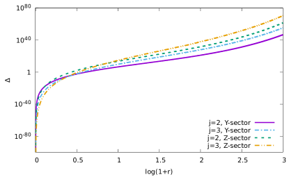
Figure 4: The Jacobi determinant for the CM monopole perturbations in the $Y$,$Z$ sectors with $j=2,3$.

Up to now we have assumed $\nu$ to be integer, but for the Abelian monopoles $\nu$ can assume also half-integer vales. The spin weights $s$ of $Y_{k}$ and $Z_{k}$ amplitudes with $k=1,2,3,4$ are then also half-integer and therefore their total angular momentum $j=|s|,|s|+1,\ldots$ is half-integer as well. It is well-known that $j$ can assume half-integer values in the presence of monopoles Brandt:1979kk . The azimuthal quantum number $m=-j,-j+1,\ldots,j$ is also half-integer, but after passing to the regular gauge with the transformation (A.12), the perturbations become proportional to $e^{i(m\pm\nu)\varphi}$ hence they are single-valued functions of $\varphi$. The above analysis then directly applies with the same conclusion: for $j=|\nu|-1$ there are unstable modes both in the $Y$ and $Z$ sectors which fulfill Eq.(8.95). Therefore, monopoles with a half-integer $\nu=3/2,5/2,\ldots$ are unstable as well. However, this conclusion does not apply to the fundamental monopole with $\nu=\pm 1/2$ because $j=|\nu|-1$ should be non-negative. Therefore, the decay channel is closed and the fundamental monopole is stable.

IX SUMMARY OF RESULTS AND CONCLUDING REMARKS

To summarize our results, we have studied spherically symmetric sector of the electroweak theory. This sector admits Abelian magnetic monopoles with magnetic charges $n=\pm 1,\pm 2,\pm 3,\ldots$ and one solution describing the non-Abelian monopole of Cho-Maison with $n=\pm 2$. All these monopoles have infinite energy due to the Colombian behaviour of the U(1) magnetic field at the origin. These solutions were known before but a systematic analysis of the electroweak spherically symmetric sector has been lacking so far. In addition, we discover spherically symmetric electroweak oscillons which were not known before, but this issue will be discussed separately GGV .

Our principal result is the analysis of the perturbative stability of the electroweak monopoles. To the best of our knowledge, this has not been done before. Our main thrust was on studying stability of the non-Abelian CM monopole, and we have found that this solution is stable. The fundamental Abelian monopole with $n=\pm 1$ is also stable, but all other Abelian monopoles are unstable. The Abelian monopole with the magnetic charge $|n|>1$ decays within the perturbative channel with angular momentum $j=|n/2|-1$. It is interesting that these properties of electroweak Abelian monopoles are very similar to those for the Abelian monopoles embedded into the pure Yang-Mills theory Yoneya:1977yi ; Brandt:1979kk .

One may wonder what the unstable monopoles decay into when perturbed. The simplest would be to think that the Abelian monopole with $|n|>1$ decays into $|n|$ fundamental monopoles, which mutually repel and fly away from each other. However, this hypothesis encounters problems already in the simplest case of $n=\pm 2$. Indeed, for the $|n|=2$ monopole to split in two, it has to be unstable with respect to dipole perturbations within the $j=1$ sector. However, it is unstable only within the $j=0$ sector and only its spherically symmetric perturbations grow in time.

Since all unstable modes of the $|n|=2$ Abelian monopole are spherically symmetric, a part of the growing perturbation will form a spherical wave and escape to infinity. The monopole will be loosing energy and will evolve toward a less energetic spherically symmetric state containing a non-Abelian condensate in its center. It should finally approach the stable CM configuration, which also has $|n|=2$. Even though the CM monopole has infinite energy, it is less energetic than the Abelian monopole since in both cases the energy is $E=E_{0}+E_{1}$ where $E_{0}$ diverges but $E_{1}$ is finite for the CM monopole and diverges for the Abelian monopole (see Eq.(IV.2)). Therefore, the CM monopole can be viewed as a stable remnant of the decay of the $|n|=2$ Abelian monopole.

One may conjecture that for the Abelian monopoles with $|n|>2$ the situation is similar and every momopole decays by emitting radiation and condensing to an equilibrium non-Abelian state. However, the monopole with $|n|>2$ decays within the sector with $j=|n/2|-1>0$, hence the final state of its evolution will be non-spherically symmetric. This suggests that the CM monopole may be just the first member of a sequence of more general and hitherto unknown non-Abelian solutions labeled by their magnetic charge $n$. Only the CM monopole is spherically symmetric while non-Abelian monopoles with $|n|>2$ should not be rotationally invariant. An attempt to show this is schematically presented in Fig.5.

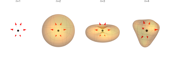
Figure 5: A schematic sketch of electroweak monopoles. The $n=1$ monopole is Abelian while the others have a non-Abelian core containing the pointlike singularity of the U(1) field in the center. Monopole solutions with $|n|=3,4,\ldots$ (not yet constructed) are not spherically symmetric.

Of course, this conjecture should be verified by explicitly constructing non-spherically symmetric solutions with $|n|>2$ (an axially symmetric solution with $n=1$ was reported in Teh:2014xva , but so far this has not been confirmed independently). At the same time, the conjecture is corroborated by the evidence obtained via taking gravity into account. Unless for quantum renormalization effects (which are unlikely to apply if $|n|\gg 1$), the energy of all flat space monopoles is infinite. Gravity provides a natural cutoff by creating an event horizon, such that all Abelian monopoles are described by the black hole geometry of Reissner-Nordstrom. It turns out that large black holes are dynamically stable, but instabilities appear for smaller black holes. Varying the horizon size, one can detect the moment when the instability just starts to appear and when it is not yet a negative mode but a zero mode GVin . Such zero modes provide the perturbative approximation for the new non-Abelian solution branches bifurcating with the Abelian branch. Starting at the bifurcation point and iteratively decreasing the event horizon size, one can construct magnetically charged hairy black holes with non-Abelian fields in the exterior region. If one wishes, one can finally send the Newton constant to zero to obtain non-Abelian solutions in flat space.

A similar observation of the stability change for magnetically charged black holes has been made within the context of a theory which is similar although not exactly identical to the electroweak theory Ridgway:1994sm ; Ridgway:1995ke ; Ridgway:1995ac . It was similarly suggested that the phenomenon could be used to construct new non-Abelian solutions without spherical symmetry. However, such a construction has never been carried out at the fully non-perturbative level.

The viewpoint that magnetic monopoles in the electroweak theory should be generically non-spherically symmetric was recently advocated by Maldacena Maldacena:2020skw , who argued that the spherically symmetric magnetic field is homogeneous on the sphere and hence should be unstable with respect to segmentation into vortices due to the Meissner effect. One may finally note that t’Hooft-Polyakov monopoles for $|n|>2$ are also not spherically symmetric Forgacs:1980ym .

APENDIX A: SPHERICALLY SYMMETRIC ELECTROWEAK FIELDS

In this Appendix we discuss equivalent forms of the spherically symmetric fields expressed by Eqs.(3.2),(3.3),(3.4) in the main text. Those expressions are convenient for calculations, but one should have in mind that both the SU(2) field (3.2) and U(1) field (3.3) are singular at the symmetry-axis where $\vartheta=0,\pi$ because their $\varphi$-components do not vanish there. It is important to check that the singularity can be removed by passing to a regular gauge, local or global, since otherwise Eqs.(3.2),(3.3),(3.4) would make no sense. It turns out that the singularity can indeed be removed, but only for special values of the parameter $\nu$ in (3.2).

The singularity in the SU(2) field (3.2) can be removed by the gauge transformation (2.6) generated by Arafune:1974uy

$${\rm U}=\exp\left(-i\nu\varphi{\rm T}_{3}\right)\exp\left(-i\vartheta{\rm T}_{2}\right)=\begin{pmatrix}\cos\frac{\vartheta}{2}\,e^{-i{\nu\varphi/2}}&~{}-\sin\frac{\vartheta}{2}\,e^{-i{\nu\varphi/2}}\\ \sin\frac{\vartheta}{2}\,e^{i{\nu\varphi/2}}~{}&~{}\cos\frac{\vartheta}{2}\,e^{i{\nu\varphi/2}}\end{pmatrix}.$$ (A.1)

This transformation is singular itself since ${\rm U}$ has no limit for $\vartheta\to 0,\pi$ but the transformed SU(2) field becomes regular in the new gauge,

$$W=(a_{0}\,dt+a_{1}\,dr){\rm T}_{r}+\left(w_{2}\,T_{\vartheta}-(1-w_{1}){\rm T}_{\varphi}\right)d\vartheta+\nu\left(w_{2}\,{\rm T}_{\varphi}+(1-w_{1})T_{\vartheta}\right)\sin\vartheta\,d\varphi.~{}~{}~{}~{}~{}~{}~{}$$ (A.2)

Here the angle-dependent generators

$${\rm T}_{r}=n^{a}{\rm T}_{a},~{}~{}~{}~{}~{}~{}{\rm T}_{\vartheta}=\partial_{\vartheta}{\rm T}_{r},~{}~{}~{}~{}~{}~{}{\rm T}_{\varphi}=\frac{1}{\nu\sin\vartheta}\,\partial_{\varphi}{\rm T}_{r}$$ (A.3)

are expressed in terms of the unit vector

$$n^{a}=\left[\,\sin\vartheta\cos(\nu\varphi),\sin\vartheta\sin(\nu\varphi),\cos\vartheta\,\right],$$ (A.4)

and it is clear that the parameter $\nu$ should be integer, since otherwise $n^{a}$ is not single-valued. For $\nu=0$ generators (A.3) are not defined, but in this case one can use the original form (3.2) which becomes regular.

For $\nu=1$, using the Cartesian coordinates $x^{a}=r\,n^{a}$, the field (A.2) can be represented in the form originally used by Witten Witten:1976ck ,

$$W={\rm T}_{a}\,n^{a}\,a_{0}dt+{\rm T}_{a}\left(a_{1}\,n^{a}n_{i}+\frac{w_{2}}{r}\,\delta^{a}_{i}+\frac{1-w_{1}}{r}\,\epsilon_{aij}\,n^{j}\right)dx^{i}\,.$$ (A.5)

The gauge transformation (A.1) does not affect the U(1) field (3.3) while the Higgs field (3.4) changes, so that in the new gauge

$$B=B_{\mu}dx^{\mu}=b_{0}\,dt+b_{1}\,dr+P\cos\vartheta\,d\varphi,~{}~{}~{}~{}~{}\Phi=\phi\,e^{i\xi/2}\begin{pmatrix}-\sin\frac{\vartheta}{2}\,e^{-i{\nu\varphi/2}}\\ \cos\frac{\vartheta}{2}\,e^{i{\nu\varphi/2}}\end{pmatrix}.$$ (A.6)

The $B$-field is singular at $\vartheta=0,\pi$ while the Higgs field has no definite value at the negative $z$-axis, for $\vartheta=\pi$, unless if $\nu=0$. However, performing an extra U(1) gauge transformation generated by

$${\rm U}=\exp\left(-\frac{i\nu\varphi}{2}\right),$$ (A.7)

the SU(2) field (A.2) does not change while the U(1) field and the Higgs field become, assuming that $P=\nu$ according to (3.9),

$$B_{+}=b_{0}\,dt+b_{1}\,dr+\nu\,(\cos\vartheta-1)\,d\varphi,~{}~{}~{}~{}~{}\Phi_{+}=\phi\,e^{i\xi/2}\begin{pmatrix}-\sin\frac{\vartheta}{2}\,e^{-i{\nu\varphi}}\\ \cos\frac{\vartheta}{2}\,\end{pmatrix}.$$ (A.8)

Both the B-field and Higgs field are now regular for $\vartheta=0$, but there is still the Dirac string singularity of the B-field at the negative $z$-axis, where $\vartheta=\pi$, whereas the Higgs field still has no limit there. Therefore, this gauge can be used only in the upper part of the sphere, for $\vartheta\in[0,\pi-\epsilon)$. However, after a further U(1) gauge transformation generated by

$${\rm U}=\exp\left(+i\nu\varphi\right)$$ (A.9)

one obtains

$$B_{-}=b_{0}\,dt+b_{1}\,dr+\nu\,(\cos\vartheta+1)\,d\varphi,~{}~{}~{}~{}~{}\Phi_{-}=\phi\,e^{i\xi/2}\begin{pmatrix}-\sin\frac{\vartheta}{2}\ \\ \cos\frac{\vartheta}{2}\,e^{+i{\nu\varphi}}\end{pmatrix},$$ (A.10)

such that the singularity is now moved to the positive $z$-axis, $\vartheta=0$, while for $\vartheta=\pi$ everything is regular. This gauge provides the regular description in the lower part of the sphere for $\vartheta\in(\epsilon,\pi]$. Therefore, the $B$ and $\Phi$ fields will be completely regular if one uses two local gauges: the gauge $B_{+},\Phi_{+}$ given by (A.8) in the upper part of the sphere and the gauge $B_{-},\Phi_{-}$ given by (A.10) in the lower part of the sphere. The transition from one local gauge to the other is performed in the equatorial region where $\epsilon<\vartheta<\pi-\epsilon$ and provided by the function (A.9) which is regular and single-valued in this region.

Summarizing, the regular form of the fields is given by (A.2) and by two local gauges (A.8) or (A.10) used, respectively, for $\vartheta\in[0,\pi-\epsilon)$ and for $\vartheta\in(\epsilon,\pi]$.

Returning back to Eqs.(3.2),(3.3),(3.4), let us finally discuss the case where $w_{1}=w_{2}=0$. Setting $P=\nu$, one has

$$W={\rm T}_{3}\,(a_{0}\,dt+a_{1}\,dr)+{\rm T}_{3}\,\nu\cos\vartheta d\varphi,~{}~{}~{}~{}~{}~{}~{}B=b_{0}\,dt+b_{1}\,dr+\nu\cos\vartheta\,d\varphi\,.$$ (A.11)

Both SU(2) and U(1) fields are singular at the symmetry axis, but after the gauge transformation generated by

$${\rm U}_{\pm}=\exp\left(\mp\frac{i\nu\varphi}{2}(1+\tau_{3})\right)$$ (A.12)

they become

$$W_{\pm} = {\rm T}_{3}\,(a_{0}\,dt+a_{1}\,dr)+{\rm T}_{3}\,\nu(\cos\vartheta\mp 1)d\varphi,~{}~{}~{}~{}~{}~{}~{}$$

$$B_{\pm} = b_{0}\,dt+b_{1}\,dr+\nu(\cos\vartheta\mp 1)\,d\varphi\,,$$ (A.13)

while the Higgs field (3.4) does not change (because it has only the lower component). The fields $W_{+},B_{+}$ are regular at $\vartheta=0$ and can be used in the northern hemisphere while $W_{-},B_{-}$ are regular at $\vartheta=\pi$ and can be used in the southern hemisphere. Using these two local gauges provides a completely regular description. The transition from $W_{+},B_{+}$ to $W_{-},B_{-}$ is provided by the gauge transformation in the equatorial region with

$${\rm U}=\exp\left(i\nu\,\varphi(1+\tau_{3})\right)=\begin{pmatrix}\exp\left(2i\,\nu\varphi\right)&0\\ 0~{}&~{}1\end{pmatrix},$$ (A.14)

which is single-valued if $\nu$ is integer or half-integer. The latter conclusion is very important, since the value $\nu=1/2$ is needed to describe the magnetic monopole with the lowest charge, which arises precisely when $w_{1}=w_{2}=0$.

The upshot of our discussion is that the fields (3.2),(3.3),(3.4) can be made regular by gauge transformations if $\nu\in\mathbb{Z}$ or when $2\nu\in\mathbb{Z}$ if $w_{1}=w_{2}=0$.

Before finishing this section, let us compare with the spherically symmetric sphaleron field. Depending on weather the SU(2) gauge field is chosen in the regular gauge (A.2) or in the singular gauge (3.2), the sphaleron Higgs field is given, respectively, by

$$\Phi_{\rm sph}^{\rm reg}=\phi\,\exp\left(i\xi\,{\rm T}_{r}\right)\begin{pmatrix}0\\ 1\end{pmatrix},~{}~{}~{}~{}~{}~{}\Phi_{\rm sph}^{\rm sing}=\phi\,\exp\left(i\xi\,{\rm T}_{3}\right)\begin{pmatrix}-\sin\frac{\theta}{2}\,e^{-\nu\phi/2}\\ \cos\frac{\theta}{2}\,e^{\nu\phi/2}\end{pmatrix}.$$ (A.15)

This is compatible with the spherical symmetry if only the Weinberg angle vanishes and the U(1) field decouples. The difference with the monopole field can also be seen in the matrix element $\langle\Phi_{\rm sph}^{\rm reg}|\tau^{a}|\Phi_{\rm sph}^{\rm reg}\rangle=-\phi^{2}\,\delta^{a}_{3}$ because for the monopole field $\Phi$ given in the regular gauge by (A.8) or (A.10) one has $\langle\Phi|\tau^{a}|\Phi\rangle=-\phi^{2}\,n^{a}$ where $n^{a}$ is the unit vector defined in (A.4).

APENDIX B: ELECTROWEAK EQUATIONS IN THE SPHERICALLY SYMMETRIC SECTOR

Injecting the ansatz (3.1)–(3.4) to the WS equations (2.8), the angular dependence separates yielding second order differential equations for functions depending on $t,r$, but also first order differential and algebraic constraints. The first algebraic constraint reads $(P-\nu)\,\phi^{2}=0$ and since $\phi\neq 0$, one should set $P=\nu$. Taking this into account, the other algebraic constraints read

$$(\nu^{2}-1)w_{a}=0,~{}~{}~{}~{}~{}~{}~{}(\nu^{2}-1)(w_{1}^{2}+w_{2}^{2}-1)\,w_{a}=0,~{}~{}~{}~{}a=1,2\,,$$ (B.1)

while the first order differential constraints are

$$(\nu^{2}-1)(\dot{w}_{1}+a_{0}\,w_{2})=0\,,~{}~{}~{}~{}~{}(\nu^{2}-1)(w^{\prime}_{1}+a_{1}\,w_{2})=0\,,$$

$$(\nu^{2}-1)(\dot{w}_{2}-a_{0}\,w_{1})=0\,,~{}~{}~{}~{}~{}(\nu^{2}-1)(w^{\prime}_{2}-a_{1}\,w_{1})=0\,.$$ (B.2)

The second order equations come from the SU(2) sector,

$$w_{1}^{\prime\prime}-\ddot{w}_{1} = \left(\frac{(w_{1}^{2}+w_{2}^{1}-1)}{r^{2}}+\frac{g^{2}\phi^{2}}{2}+a_{1}^{2}-a_{0}^{2}\right)w_{1}+2\,(a_{0}\,\dot{w}_{2}-a_{1}w_{2}^{\prime})+(\dot{a}_{0}-a_{1}^{\prime})\,w_{2}\,,$$

$$w_{2}^{\prime\prime}-\ddot{w}_{2} = \left(\frac{(w_{1}^{2}+w_{2}^{1}-1)}{r^{2}}+\frac{g^{2}\phi^{2}}{2}+a_{1}^{2}-a_{0}^{2}\right)w_{2}-2\,(a_{0}\,\dot{w}_{1}-a_{1}w_{1}^{\prime})-(\dot{a}_{0}-a_{1}^{\prime})\,w_{1}\,,$$

$$\left(r^{2}(a_{0}^{\prime}-\dot{a}_{1})\right)^{\prime} = \frac{g^{2}r^{2}\phi^{2}}{2}\left(a_{0}-b_{0}+\dot{\xi}\right)+2\left[(w_{1}^{2}+w_{2}^{2})\,a_{0}+\dot{w}_{1}\,w_{2}-\dot{w}_{2}\,w_{1}\right]\,,$$

$$\left(r^{2}(a_{0}^{\prime}-\dot{a}_{1})\right)^{\mbox{$\cdot$}} = \frac{g^{2}r^{2}\phi^{2}}{2}\left(a_{1}-b_{1}+\xi^{\prime}\right)+2\left[(w_{1}^{2}+w_{2}^{2})\,a_{1}+w^{\prime}_{1}\,w_{2}-w^{\prime}_{2}\,w_{1}\right]\,,$$ (B.3)

from the U(1) sector,

$$\left(r^{2}(b_{0}^{\prime}-\dot{b}_{1})\right)^{\prime}+\frac{g^{\prime 2}r^{2}\phi^{2}}{2}\left(a_{0}-b_{0}+\dot{\xi}\right) = 0\,,$$

$$\left(r^{2}(b_{0}^{\prime}-\dot{b}_{1})\right)^{\mbox{$\cdot$}}+\frac{g^{\prime 2}r^{2}\phi^{2}}{2}\left(a_{1}-b_{1}+\xi^{\prime}\right) = 0\,,$$ (B.4)

and from the Higgs sector,

$$\frac{1}{r^{2}}\left(r^{2}\phi^{\prime}\right)^{\prime}-\ddot{\phi}=\left(\beta\,(\phi^{2}-1)+\left(a_{1}-b_{1}+\xi^{\prime}\right)^{2}-\left(a_{0}-b_{0}+\dot{\xi}\right)^{2}+\frac{2}{r^{2}}\,(w_{1}^{2}+w_{2}^{2})\right)\frac{\phi}{4}\,,$$

$$\left(r^{2}\phi^{2}(a_{1}-b_{1}+\xi^{\prime})\right)^{\prime}=\left(r^{2}\phi^{2}(a_{0}-b_{0}+\dot{\xi})\right)^{\mbox{$\cdot$}}\,.~{}~{}~{}~{}~{}~{}~{}~{}$$ (B.5)

These equations can be simplified by setting

$$w_{1} = f\,\cos\alpha,~{}~{}~{}w_{2}=f\,\sin\alpha,~{}~{}~{}~{}a_{0}=\Omega_{0}+\dot{\alpha},~{}~{}~{}a_{1}=\Omega_{1}+\alpha^{\prime},~{}~{}~{}$$

$$b_{0} = \dot{\xi}+a_{0}-\Theta_{0},~{}~{}~{}~{}~{}b_{1}={\xi}^{\prime}+a_{1}-\Theta_{1}\,,$$ (B.6)

where $f,\alpha,\Omega_{0},\Omega_{1},\Theta_{0},\Theta_{1}$ are functions of $t,r$. The amplitudes $\alpha,\xi$ correspond to pure gauge degrees of freedom and drop out from the equations, which leads to Eqs.(III)–(3.14) in the main text. It is not difficult to see that the algebraic and first order differential constraints (B.1),(APENDIX B: ELECTROWEAK EQUATIONS IN THE SPHERICALLY SYMMETRIC SECTOR) leave only two options: either $\nu^{2}=1$ or $w_{1}=w_{2}=0$, which can be expressed by the condition $(\nu^{2}-1)\,f=0$ shown in Eq.(3.10) in the main text.

APENDIX C: PERTURBATION EQUATIONS AFTER VARIABLE SEPARATION

In this Appendix we show the radial equations obtained by inserting the ansatz (6.48)–(6.52) into the perturbation equations (6.37) and separating the angular and temporal variables. There are altogether 20 coupled ordinary differential equations for the 20 radial amplitudes $S_{0}(r),\ldots,$ $X_{10}(r),\ldots,$ $H_{1}(r),\ldots,H_{4}(r)$. Defining the quantities

$${\cal C}_{1} =\frac{\left(rX_{11}\right)^{\prime}}{r}-\omega\,X_{10}+\frac{j-\nu_{-}}{\sqrt{2}\,r}\,X_{12}-\frac{j+\nu_{+}}{\sqrt{2}\,r}\,X_{13}-\frac{\nu_{-}\,f}{\sqrt{2}\,r}\,X_{32}+\frac{\nu_{+}\,f}{\sqrt{2}\,r}\,X_{33}+g^{2}\phi\,H_{1}\,,$$ (C.1a)

$${\cal C}_{2} =\frac{\left(rX_{21}\right)^{\prime}}{r}-\omega\,X_{20}+\frac{j+\nu_{+}}{\sqrt{2}\,r}\,X_{22}-\frac{j-\nu_{-}}{\sqrt{2}\,r}\,X_{23}+\frac{\nu_{+}\,f}{\sqrt{2}\,r}\,X_{32}-\frac{\nu_{-}\,f}{\sqrt{2}\,r}\,X_{33}-g^{2}\phi\,H_{2}\,,$$ (C.1b)

$${\cal C}_{3} =\frac{\left(rX_{31}\right)^{\prime}}{r}-\omega\,X_{30}+\frac{\nu_{-}\,f}{2\sqrt{2}\,r}\,(X_{13}+X_{22})-\frac{\nu_{+}\,f}{2\sqrt{2}\,r}\,(X_{12}+X_{23})$$

$$\hskip 199.16928pt+\frac{j+1}{\sqrt{2}\,r}\,(X_{32}-X_{33})+\frac{g^{2}}{2}\,\phi\,(H_{4}-H_{3})\,,$$ (C.1c)

$${\cal C}_{4} =\frac{\left(rS_{1}\right)^{\prime}}{r}-\omega\,S_{0}+\frac{j+1}{\sqrt{2}\,r}\,(S_{2}-S_{3})+\frac{g^{\prime 2}}{2}\,\phi\,(H_{3}-H_{4})\,,$$ (C.1d)

where $\nu_{\pm}\equiv\nu\pm 1$, the 4 equations for the SU(2) amplitudes $X_{1\alpha}(r)$ can be represented in the form

$$~{}~{}~{}\hat{{\cal D}}X_{10}+\frac{2\nu\,j\,f}{r^{2}}\,X_{30}=-\omega\,{\cal C}_{1}\,,$$ (C.2a)

$$\left(\hat{{\cal D}}-\frac{2}{r^{2}}\right)X_{11}+\frac{2\nu\,j\,f}{r^{2}}\,X_{31}-\frac{\sqrt{2}\,(j-\nu_{-})}{r^{2}}\,X_{12}+\frac{\sqrt{2}\,(j+\nu_{+})}{r^{2}}\,X_{13}$$

$$~{}~{}~{}+\left(\frac{\sqrt{2}\,f}{r}\right)^{\prime}\left(\nu_{+}X_{33}-\nu_{-}X_{32}\right)+2g^{2}\phi^{\prime}\,H_{1}=r\left(\frac{{\cal C}_{1}}{r}\right)^{\prime}\,,$$ (C.2b)

$$\left(\hat{{\cal D}}-\frac{2\nu f^{2}}{r^{2}}\right)X_{12}-\frac{\sqrt{2}\,(j+\nu)}{r^{2}}\,X_{11}-\left(\frac{\sqrt{2}\,\nu_{+}\,f}{r}\right)^{\prime}X_{31}+\frac{2(\nu j+1)\,f}{r^{2}}\,X_{32}$$

$$~{}~{}~{}+\frac{\nu_{+}\,g^{2}f\,\phi}{\sqrt{2}\,r}\,H_{4}=\frac{\nu_{+}\,f\,{\cal C}_{3}-(j+\nu)\,{\cal C}_{1}}{\sqrt{2}\,r}\,,$$ (C.2c)

$$\left(\hat{{\cal D}}+\frac{2\nu f^{2}}{r^{2}}\right)X_{13}+\frac{\sqrt{2}\,(j-\nu)}{r^{2}}\,X_{11}+\left(\frac{\sqrt{2}\,\nu_{-}\,f}{r}\right)^{\prime}X_{31}+\frac{2(\nu j-1)\,f}{r^{2}}\,X_{33}$$

$$~{}~{}~{}-\frac{\nu_{-}\,g^{2}f\,\phi}{\sqrt{2}\,r}\,H_{4}=\frac{(j-\nu)\,{\cal C}_{1}-\nu_{-}\,f\,{\cal C}_{3}}{\sqrt{2}\,r}\,,$$ (C.2d)

with the differential operator

$$\hat{{\cal D}}\equiv\frac{d^{2}}{dr^{2}}+\omega^{2}-\frac{j(j+1)}{r^{2}}-\frac{g^{2}\phi^{2}}{2}\,+\frac{\nu^{2}-f^{2}}{r^{2}}.$$ (C.3)

The 4 equations for $X_{2\alpha}(r)$ read

$$~{}~{}~{}~{}~{}\hat{{\cal D}}X_{20}-\frac{2\nu\,j\,f}{r^{2}}\,X_{30}=-\omega\,{\cal C}_{2}\,,$$ (C.4a)

$$\left(\hat{{\cal D}}-\frac{2}{r^{2}}\right)X_{21}-\frac{2\nu\,j\,f}{r^{2}}\,X_{31}-\frac{\sqrt{2}\,(j+\nu_{+})}{r^{2}}\,X_{22}+\frac{\sqrt{2}\,(j-\nu_{-})}{r^{2}}\,X_{23}$$

$$~{}~{}~{}+\left(\frac{\sqrt{2}\,f}{r}\right)^{\prime}\left(\nu_{+}X_{32}-\nu_{-}X_{33}\right)-2g^{2}\phi^{\prime}\,H_{2}=r\left(\frac{{\cal C}_{2}}{r}\right)^{\prime}\,,$$ (C.4b)

$$\left(\hat{{\cal D}}+\frac{2\nu f^{2}}{r^{2}}\right)X_{22}-\frac{\sqrt{2}\,(j-\nu)}{r^{2}}\,X_{21}+\left(\frac{\sqrt{2}\,\nu_{-}\,f}{r}\right)^{\prime}X_{31}-\frac{2(\nu j-1)\,f}{r^{2}}\,X_{32}$$

$$~{}~{}~{}+\frac{\nu_{-}\,g^{2}f\,\phi}{\sqrt{2}\,r}\,H_{3}=-\frac{(j-\nu)\,{\cal C}_{2}+\nu_{-}\,f\,{\cal C}_{3}}{\sqrt{2}\,r}\,,\$$ (C.4c)

$$\left(\hat{{\cal D}}-\frac{2\nu f^{2}}{r^{2}}\right)X_{23}+\frac{\sqrt{2}\,(j+\nu)}{r^{2}}\,X_{21}-\left(\frac{\sqrt{2}\,\nu_{+}\,f}{r}\right)^{\prime}X_{31}-\frac{2(\nu j+1)\,f}{r^{2}}\,X_{33}$$

$$~{}~{}~{}-\frac{\nu_{+}\,g^{2}f\,\phi}{\sqrt{2}\,r}\,H_{3}=\frac{(j+\nu)\,{\cal C}_{2}+\nu_{+}\,f\,{\cal C}_{3}}{\sqrt{2}\,r}\,,$$ (C.4d)

the 4 equations for $X_{3\alpha}(r)$ are

$$\left(\hat{{\cal D}}-\frac{f^{2}+\nu^{2}}{r^{2}}\right)X_{30}+\frac{\nu\,(j+1)\,f}{r^{2}}\,(X_{10}-X_{20})+\frac{g^{2}\phi^{2}}{2}\,S_{0}=-\omega\,{\cal C}_{3}\,,$$ (C.5a)

$$\left(\hat{{\cal D}}-\frac{f^{2}+\nu^{2}+2}{r^{2}}\right)X_{31}+\frac{\nu\,(j+1)\,f}{r^{2}}\,(X_{11}-X_{21})-\left(\frac{\nu_{+}\,f}{\sqrt{2}\,r}\right)^{\prime}(X_{12}+X_{23})\,$$ (C.5b)

$$~{}+\left(\frac{\nu_{-}\,f}{\sqrt{2}\,r}\right)^{\prime}(X_{13}+X_{22})+\frac{\sqrt{2}\,(j+1)}{r^{2}}\,(X_{33}-X_{32})+\frac{g^{2}\phi^{2}}{2}\,S_{1}+g^{2}\,\phi^{\prime}\,(H_{4}-H_{3})=r\left(\frac{{\cal C}_{3}}{r}\right)^{\prime}\,,$$

$$\left(\hat{{\cal D}}-\frac{f^{2}+\nu^{2}}{r^{2}}\right)X_{32}+\left(\frac{f}{\sqrt{2}\,r}\right)^{\prime}\left(\nu_{+}\,X_{21}-\nu_{-}\,X_{11}\right)+\frac{[(j+1)\nu-1]\,f}{r^{2}}\,X_{12}-\frac{[(j+1)\nu+1]\,f}{r^{2}}\,X_{22}\,$$

$$~{}~{}~{}-\frac{\sqrt{2}\,j}{r^{2}}\,X_{31}+\frac{g^{2}\phi^{2}}{2}\,S_{2}+\frac{g^{2}\,f\,\phi}{2\sqrt{2}\,r}\,(\nu_{-}\,H_{1}+\nu_{+}\,H_{2})=\frac{f\left(\nu_{-}\,{\cal C}_{1}-\nu_{+}\,{\cal C}_{2}\right)}{2\sqrt{2}\,r}\,-\frac{j\,{\cal C}_{3}}{\sqrt{2}\,r}\,,$$ (C.5c)

$$\left(\hat{{\cal D}}-\frac{f^{2}+\nu^{2}}{r^{2}}\right)X_{33}+\left(\frac{f}{\sqrt{2}\,r}\right)^{\prime}\left(\nu_{+}\,X_{11}-\nu_{-}\,X_{21}\right)+\frac{(\nu_{+}\,j+1)\,f}{r^{2}}\,X_{13}-\frac{(\nu_{+}\,j-1)\,f}{r^{2}}\,X_{23}\,$$

$$~{}~{}~{}+\frac{\sqrt{2}\,j}{r^{2}}\,X_{31}+\frac{g^{2}\phi^{2}}{2}\,S_{3}-\frac{g^{2}\,f\,\phi}{2\sqrt{2}\,r}\,(\nu_{+}\,H_{1}+\nu_{-}\,H_{2})=\frac{f\left(\nu_{-}\,{\cal C}_{2}-\nu_{+}\,{\cal C}_{1}\right)}{2\sqrt{2}\,r}\,+\frac{j\,{\cal C}_{3}}{\sqrt{2}\,r}\,,$$ (C.5d)

the equations for the U(1) amplitudes are

$$\hat{{\cal D}}_{s}\,S_{0}+\frac{g^{\prime 2}\phi^{2}}{2}\,X_{30}=-\omega\,{\cal C}_{4}\,,$$ (C.6a)

$$\left(\hat{{\cal D}}_{s}-\frac{2}{r^{2}}\right)\,S_{1}+\frac{g^{\prime 2}\phi^{2}}{2}\,X_{31}+\frac{\sqrt{2}\,(j+1)}{r^{2}}\,(S_{3}-S_{2})+g^{\prime 2}\phi^{\prime}\,(H_{3}-H_{4})=r\left(\frac{{\cal C}_{4}}{r}\right)^{\prime}\,,$$ (C.6b)

$$\hat{{\cal D}}_{s}\,S_{2}+\frac{g^{\prime 2}\phi^{2}}{2}\,X_{32}-\frac{\sqrt{2}\,j}{r^{2}}\,S_{1}+\frac{g^{\prime 2}f\,\phi}{2\sqrt{2}\,r}\,(\nu_{-}H_{1}+\nu_{+}H_{2})=-\frac{j\,{\cal C}_{4}}{\sqrt{2}\,r}\,,$$ (C.6c)

$$\hat{{\cal D}}_{s}\,S_{3}+\frac{g^{\prime 2}\phi^{2}}{2}\,X_{33}+\frac{\sqrt{2}\,j}{r^{2}}\,S_{1}-\frac{g^{\prime 2}f\,\phi}{2\sqrt{2}\,r}\,(\nu_{+}H_{1}+\nu_{-}H_{2})=\frac{j\,{\cal C}_{4}}{\sqrt{2}\,r}\,,$$ (C.6d)

and the equations for the Higgs amplitudes are

$$\left(\hat{{\cal D}}+\frac{f^{2}}{2r^{2}}+\frac{\beta}{4}(1-\phi^{2})\right)H_{1}-\frac{\nu jf}{r^{2}}\,H_{3}+\phi^{\prime}X_{11}$$ (C.7a)

$$~{}~{}~{}\hskip 184.9429pt+\frac{\nu_{-}\,f\,\phi}{2\sqrt{2}\,r}\,(S_{2}+X_{32})-\frac{\nu_{+}\,f\,\phi}{2\sqrt{2}\,r}\,(S_{3}+X_{33})=-\frac{\phi\,{\cal C}_{1}}{2}\,,$$

$$\left(\hat{{\cal D}}+\frac{f^{2}}{2r^{2}}+\frac{\beta}{4}(1-\phi^{2})\right)H_{2}+\frac{\nu jf}{r^{2}}\,H_{4}-\phi^{\prime}X_{21}$$ (C.7b)

$$~{}~{}~{}\hskip 184.9429pt+\frac{\nu_{+}\,f\,\phi}{2\sqrt{2}\,r}\,(S_{2}+X_{32})-\frac{\nu_{-}\,f\,\phi}{2\sqrt{2}\,r}\,(S_{3}+X_{33})=\frac{\phi\,{\cal C}_{2}}{2}\,,$$

$$\hat{{\cal D}}_{h}\,H_{3}+\frac{f\,\phi}{2\sqrt{2}\,r}\,(\nu_{-}X_{22}-\nu_{+}X_{23})-\phi^{\prime}(X_{31}-S_{1})$$ (C.7c)

$$~{}~{}~{}\hskip 170.71652pt-\frac{\nu\,(j+1)\,f}{r^{2}}\,H_{1}+\frac{(1-\beta)\,\phi^{2}}{4}\,H_{4}=\frac{\phi}{2}\,({\cal C}_{3}-{\cal C}_{4})\,,$$

$$\hat{{\cal D}}_{h}\,H_{4}+\frac{f\,\phi}{2\sqrt{2}\,r}\,(\nu_{+}X_{12}-\nu_{-}X_{13})+\phi^{\prime}(X_{31}-S_{1})$$ (C.7d)

$$~{}~{}~{}\hskip 170.71652pt+\frac{\nu\,(j+1)\,f}{r^{2}}\,H_{2}+\frac{(1-\beta)\,\phi^{2}}{4}\,H_{3}=\frac{\phi}{2}\,({\cal C}_{4}-{\cal C}_{3})\,,$$

with the differential operators

$$\hat{{\cal D}}_{s} = \frac{d^{2}}{dr^{2}}+\omega^{2}-\frac{j(j+1)}{r^{2}}-\frac{g^{\prime 2}\phi^{2}}{2},~{}$$

$$\hat{{\cal D}}_{h} = \frac{d^{2}}{dr^{2}}+\omega^{2}-\frac{j(j+1)}{r^{2}}-\frac{f^{2}}{2r^{2}}+\frac{\beta}{4}-\frac{1}{4}\,(1+2\beta)\,\phi^{2}\,.$$ (C.8)

These equations are invariant under gauge transformations (7.55)–(7.59). As discussed in the main text, imposing the harmonic gauge conditions ${\cal C}_{1}={\cal C}_{2}={\cal C}_{3}={\cal C}_{4}=0$ reduces the number of independent equations to 16 which can be split into two independent subsystems of 7 and 9 equations.

APENDIX D: PERTURBATION POTENTIALS

In this Appendix we show the explicit expression for components of the $7\times 7$ matrix potential $\hat{U}$ and for the $9\times 9$ matrix potential $\hat{V}$ in the Schroedinger-type equations (7.71). These potentials are symmetric matrices. The components of $\hat{U}$ are

$$U_{11} = \frac{j(j+1)-\nu^{2}}{r^{2}}+\frac{(1+2\nu)\,f^{2}}{r^{2}}+\frac{g^{2}\phi^{2}}{2}\,,~{}~{}U_{12}=\frac{\sqrt{2}\,(j+\nu)}{\kappa_{+}\,r^{2}}\,,~{}~{}U_{13}=U_{14}=0\,,$$

$$U_{15} = \frac{g\,\sqrt{2}\,(1+\nu\,j)\,f}{\kappa_{+}\,r^{2}}\,,~{}~{}~{}U_{16}=-\frac{g^{\prime}\,\sqrt{2}\,(1+\nu\,j)\,f}{\kappa_{+}\,r^{2}}\,,~{}~{}~{}U_{17}=-\frac{g\,\nu_{+}\,f\,\phi}{2\kappa\,\kappa_{+}\,r}\,,$$

$$U_{22} = \frac{j(j+1)+2-\nu^{2}}{r^{2}}+\frac{f^{2}}{r^{2}}+\frac{g^{2}\phi^{2}}{2}\,,~{}~{}~{}~{}~{}U_{23}=-g\sqrt{2}\,\phi^{\prime}\,,~{}~{}~{}U_{24}=-\frac{\sqrt{2}\,\kappa_{-}\,(j+\nu_{+})}{r^{2}}\,,~{}~{}~{}~{}~{}$$

$$U_{25} = 2g\,\left(\frac{f}{r}\right)^{\prime}\,,~{}~{}~{}~{}~{}U_{26}=-2g^{\prime}\,\left(\frac{f}{r}\right)^{\prime}\,,~{}~{}~{}~{}~{}U_{27}=0\,,$$

$$U_{33} = \frac{j(j+1)-\nu^{2}}{r^{2}}+\frac{f^{2}}{2r^{2}}+\frac{g^{2}\phi^{2}}{2}+\frac{\beta}{4}(\phi^{2}-1)\,,~{}~{}~{}~{}U_{34}=0\,,$$

$$U_{35} = \frac{(g^{\prime 2}-g^{2})\,f\,\phi}{\sqrt{2}\,r},~{}~{}~{}U_{36}=\frac{\sqrt{2}\,gg^{\prime}\,f\,\phi}{r},~{}~{}~{}~{}~{}~{}U_{37}=\frac{\nu\,\sqrt{j(j+1)}\,f}{r^{2}}\,,$$

$$U_{44} = \frac{j(j+1)-\nu^{2}}{r^{2}}+\frac{(1-2\nu)\,f^{2}}{r^{2}}+\frac{g^{2}\phi^{2}}{2}\,,~{}~{}~{}~{}~{}$$

$$U_{45} = \frac{\sqrt{2}\,g\,(\nu\,j-1)\,f}{\kappa_{-}\,r^{2}}\,,~{}~{}~{}U_{46}=\frac{\sqrt{2}\,g^{\prime}\,(1-\nu\,j)\,f}{\kappa_{-}\,r^{2}}\,,~{}~{}~{}U_{47}=\frac{g\nu_{-}\,f\,\phi}{2\kappa\kappa_{-}\,r}\,,~{}~{}~{}~{}~{}~{}~{}$$

$$U_{55} = \frac{j(j+1)}{r^{2}}+\frac{2g^{2}\,f^{2}}{r^{2}}+\frac{\phi^{2}}{2}\,,~{}~{}~{}U_{56}=-\frac{2\,gg^{\prime}\,f^{2}}{r^{2}}\,,~{}~{}~{}~{}U_{57}=0\,,~{}~{}$$

$$U_{66} = \frac{j(j+1)}{r^{2}}+\frac{2g^{\prime 2}\,f^{2}}{r^{2}}\,,~{}~{}~{}~{}U_{67}=0,~{}~{}~{}~{}U_{77}=\frac{j(j+1)}{r^{2}}+\frac{f^{2}}{2r^{2}}+\frac{\beta}{4}\,(3\phi^{2}-1).$$ (D.1)

The components of $\hat{V}$ read

$$V_{11} = \frac{j(j+1)-\nu^{2}}{r^{2}}+\frac{(1+2\nu)\,f^{2}}{r^{2}}+\frac{g^{2}\phi^{2}}{2}\,,~{}~{}V_{12}=\frac{\sqrt{2}\,(j+\nu)}{\kappa_{+}\,r^{2}}\,,~{}~{}V_{13}=V_{14}=0\,,$$

$$V_{15} = -\frac{g\,\nu_{+}\,f\,\phi}{2\kappa\,\kappa_{+}\,r}\,,~{}~{}~{}~{}V_{16}=-\frac{\sqrt{2}\,g\,\nu_{+}}{\kappa\kappa_{+}}\,\left(\frac{f}{r}\right)^{\prime}\,,~{}~{}~{}~{}~{}V_{17}=\frac{\sqrt{2}\,g\,(1+\nu j)\,f}{\kappa_{+}\,r^{2}}$$

$$V_{18} = \frac{\sqrt{2}\,g^{\prime}\,\nu_{+}}{\kappa\kappa_{+}}\,\left(\frac{f}{r}\right)^{\prime}\,,~{}~{}~{}~{}~{}V_{19}=-\frac{\sqrt{2}\,g^{\prime}\,(1+\nu j)\,f}{\kappa_{+}\,r^{2}}\,,$$

$$V_{22} = \frac{j(j+1)+2-\nu^{2}}{r^{2}}+\frac{f^{2}}{r^{2}}+\frac{g^{2}\phi^{2}}{2}\,,~{}~{}~{}~{}~{}V_{23}=\sqrt{2}\,g\,\phi^{\prime}\,,~{}~{}~{}V_{24}=-\frac{\sqrt{2}\,\kappa_{-}\,(j+\nu_{+})}{r^{2}}\,,~{}~{}~{}~{}~{}$$

$$V_{25} = 0,~{}~{}~{}V_{26}=\frac{2g\,\kappa\,(j+1)\,\nu f}{r^{2}},~{}~{}~{}~{}V_{27}=-2g\nu\,\left(\frac{f}{r}\right)^{\prime}\,,~{}~{}~{}~{}~{}$$

$$V_{28} = -\frac{2g^{\prime}\nu\sqrt{j(j+1)}\,f}{r^{2}}\,,~{}~{}~{}~{}V_{29}=2g^{\prime}\nu\,\left(\frac{f}{r}\right)^{\prime},$$

$$V_{33} = \frac{j(j+1)-\nu^{2}}{r^{2}}+\frac{f^{2}}{2r^{2}}+\frac{g^{2}\phi^{2}}{2}+\frac{\beta}{4}\,(\phi^{2}-1)\,,~{}~{}~{}~{}V_{34}=0\,,~{}~{}~{}~{}V_{35}=\frac{\nu\,\sqrt{j(j+1)}\,f}{r^{2}}\,$$

$$V_{36} = 0,~{}~{}~{}V_{37}=\frac{(g^{\prime 2}-g^{2})\,\nu\,f\,\phi}{\sqrt{2}\,r},~{}~{}~{}V_{38}=0\,,~{}~{}~{}~{}V_{39}=\frac{\sqrt{2}\,gg^{\prime}\nu\,f\,\phi}{r},$$

$$V_{44} = \frac{j(j+1)-\nu^{2}}{r^{2}}+\frac{(1-2\nu)\,f^{2}}{r^{2}}+\frac{g^{2}\phi^{2}}{2}\,,~{}~{}~{}~{}~{}V_{45}=\frac{g\nu_{-}f\,\phi}{2\kappa\kappa_{-}\,r}\,,~{}~{}~{}~{}~{}V_{46}=\frac{\sqrt{2}\,g\,\nu_{-}}{\kappa\kappa_{-}}\,\left(\frac{f}{r}\right)^{\prime}\,,~{}$$

$$V_{47} = -\frac{\sqrt{2}\,g\,(\nu\,j-1)\,f}{\kappa_{-}\,r^{2}}\,,~{}~{}~{}V_{48}=-\frac{\sqrt{2}\,g^{\prime}\,\nu_{-}}{\kappa\kappa_{-}}\,\left(\frac{f}{r}\right)^{\prime}\,,~{}~{}~{}~{}V_{49}=\frac{\sqrt{2}\,g^{\prime}\,(\nu\,j-1)\,f}{\kappa_{-}\,r^{2}}\,,~{}~{}~{}~{}~{}~{}~{}$$

$$V_{55} = \frac{j(j+1)}{r^{2}}+\frac{f^{2}}{2r^{2}}+\frac{\phi^{2}}{2}+\frac{\beta}{4}\,(\phi^{2}-1),~{}~{}~{}V_{56}=\sqrt{2}\,\phi^{\prime},~{}~{}~{}V_{57}=V_{58}=V_{59}=0\,,$$

$$V_{66} = \frac{j(j+1)+2}{r^{2}}+\frac{2g^{2}\,f^{2}}{r^{2}}+\frac{\phi^{2}}{2}\,,~{}~{}~{}V_{67}=\frac{2\sqrt{j(j+1)}}{r^{2}}\,,~{}~{}V_{68}=-\frac{2\,gg^{\prime}\,f^{2}}{r^{2}}\,,~{}~{}~{}~{}V_{69}=0\,,~{}~{}$$

$$V_{77} = \frac{j(j+1)}{r^{2}}+\frac{2g^{2}\,f^{2}}{r^{2}}+\frac{\phi^{2}}{2}\,,~{}~{}~{}~{}V_{78}=0,~{}~{}~{}~{}V_{79}=-\frac{2gg^{\prime}\,f^{2}}{r^{2}}\,,$$

$$V_{88} = \frac{j(j+1)+2}{r^{2}}+\frac{2g^{\prime 2}\,f^{2}}{r^{2}}\,,~{}~{}~{}~{}V_{89}=\frac{2\sqrt{j(j+1)}}{r^{2}},~{}~{}~{}~{}~{}V_{99}=\frac{j(j+1)}{r^{2}}+\frac{2g^{\prime 2}f^{2}}{r^{2}}.$$ (D.2)

References

- (1) P. A. M. Dirac, Quantised singularities in the electromagnetic field,, Proc. Roy. Soc. Lond. A 133 (1931), no. 821 60–72, [doi:10.1098/rspa.1931.0130].
- (2) T. T. Wu and C. N. Yang, Dirac monopole without strings: monopole harmonics, Nucl. Phys. B 107 (1976) 365, [doi:10.1016/0550-3213(76)90143-7].
- (3) T. T. Wu and C. N. Yang, Some solutions of the classical isotopic gauge field equations, in Properties of Matter Under Unusual Conditions (H. Mark, S. Fernbach, ed.), pp. 344–354. Wiley-Interscience, 1969.
- (4) G. ’t Hooft, Magnetic monopoles in unified gauge theories, Nucl. Phys. B 79 (1974) 276–284, [doi:10.1016/0550-3213(74)90486-6].
- (5) A. M. Polyakov, Particle spectrum in quantum field theory, JETP Lett. 20 (1974) 194–195.
- (6) P. Goddard and D. I. Olive, New developments in the theory of magnetic monopoles, Rept. Prog. Phys. 41 (1978) 1357, [doi:10.1088/0034-4885/41/9/001].
- (7) S. R. Coleman, The magnetic monopole fifty years later, in Les Houches Summer School of Theoretical Physics: Laser-Plasma Interactions, pp. 461–552, 6, 1982.
- (8) K. Konishi, The magnetic monopoles seventy-five years later, Lect. Notes Phys. 737 (2008) 471–521, [arXiv:hep-th/0702102].
- (9) N. S. Manton and P. Sutcliffe, Topological solitons. Cambridge Monographs on Mathematical Physics. Cambridge University Press, 2004.
- (10) Y. M. Shnir, Magnetic Monopoles. Text and Monographs in Physics. Springer, Berlin/Heidelberg, 2005.
- (11) A. H. Chamseddine and M. S. Volkov, NonAbelian BPS monopoles in N=4 gauged supergravity, Phys. Rev. Lett. 79 (1997) 3343–3346, [arXiv:hep-th/9707176], [doi:10.1103/PhysRevLett.79.3343].
- (12) P. Forgacs and M. S. Volkov, Resonant excitations of the ’t Hooft-Polyakov monopole, Phys. Rev. Lett. 92 (2004) 151802, [arXiv:hep-th/0311062], [doi:10.1103/PhysRevLett.92.151802].
- (13) A. Rajantie, The search for magnetic monopoles, Phys. Today 69 (2016), no. 10 40–46, [doi:10.1063/PT.3.3328].
- (14) V. A. Mitsou, Searches for magnetic monopoles: a review, MDPI Proc. 13 (2019), no. 1 10, [doi:10.3390/proceedings2019013010].
- (15) F. R. Klinkhamer and N. S. Manton, A saddle point solution in the Weinberg-Salam theory, Phys. Rev. D 30 (1984) 2212, [doi:10.1103/PhysRevD.30.2212].
- (16) B. Kleihaus, J. Kunz, and Y. Brihaye, The electroweak sphaleron at physical mixing angle, Phys. Lett. B 273 (1991) 100–104, [doi:10.1016/0370-2693(91)90560-D].
- (17) R. F. Dashen, B. Hasslacher, and A. Neveu, Nonperturbative methods and extended hadron models in field theory. 3. Four-dimensional nonabelian models, Phys. Rev. D 10 (1974) 4138, [doi:10.1103/PhysRevD.10.4138].
- (18) L. G. Yaffe, Static solutions of SU(2) Higgs theory, Phys. Rev. D 40 (1989) 3463, [doi:10.1103/PhysRevD.40.3463].
- (19) B. Ratra and L. G. Yaffe, Spherically symmetric classical solutions in SU(2) gauge theory with a Higgs field, Phys. Lett. B 205 (1988) 57–61, [doi:10.1016/0370-2693(88)90398-X].
- (20) E. Farhi, N. Graham, V. Khemani, R. Markov, and R. Rosales, An oscillon in the SU(2) gauged Higgs model, Phys. Rev. D 72 (2005) 101701, [arXiv:hep-th/0505273], [doi:10.1103/PhysRevD.72.101701].
- (21) N. Graham, An electroweak oscillon, Phys. Rev. Lett. 98 (2007) 101801, [arXiv:hep-th/0610267], [doi:10.1103/PhysRevLett.98.101801]. [Erratum: Phys.Rev.Lett. 98, 189904 (2007)].
- (22) N. Graham, Numerical simulation of an electroweak oscillon, Phys. Rev. D 76 (2007) 085017, [arXiv:0706.4125], [doi:10.1103/PhysRevD.76.085017].
- (23) Y. M. Cho and D. Maison, Monopoles in Weinberg-Salam model, Phys. Lett. B 391 (1997) 360–365, [arXiv:hep-th/9601028], [doi:10.1016/S0370-2693(96)01492-X].
- (24) Y. M. Cho, K. Kim, and J. H. Yoon, Finite energy electroweak dyon, Eur. Phys. J. C 75 (2015), no. 2 67, [arXiv:1305.1699], [doi:10.1140/epjc/s10052-015-3290-3].
- (25) D. G. Pak, P. M. Zhang, and L. P. Zou, On finite energy monopole solutions in Weinberg–Salam model, Int. J. Mod. Phys. A 30 (2015), no. 27 1550164, [arXiv:1311.7567], [doi:10.1142/S0217751X1550164X].
- (26) F. Blaschke and P. Beneš, BPS Cho–Maison monopole, PTEP 2018 (2018), no. 7 073B03, [arXiv:1711.04842], [doi:10.1093/ptep/pty071].
- (27) J. Ellis, P. Q. Hung, and N. E. Mavromatos, An electroweak monopole, Dirac quantization and the weak mixing angle, Nucl. Phys. B 969 (2021) 115468, [arXiv:2008.00464], [doi:10.1016/j.nuclphysb.2021.115468].
- (28) P. Q. Hung, Topologically stable, finite-energy electroweak-scale monopoles, Nucl. Phys. B 962 (2021) 115278, [arXiv:2003.02794], [doi:10.1016/j.nuclphysb.2020.115278].
- (29) Y. Bai and M. Korwar, Hairy magnetic and dyonic black holes in the Standard Model, JHEP 04 (2021) 119, [arXiv:2012.15430], [doi:10.1007/JHEP04(2021)119].
- (30) E. Witten, Some exact multi - instanton solutions of classical Yang-Mills theory, Phys. Rev. Lett. 38 (1977) 121–124, [doi:10.1103/PhysRevLett.38.121].
- (31) Y. Nambu, String-like configurations in the Weinberg-Salam theory, Nucl. Phys. B 130 (1977) 505, [doi:10.1016/0550-3213(77)90252-8].
- (32) T. Vachaspati, Vortex solutions in the Weinberg-Salam model, Phys. Rev. Lett. 68 (1992) 1977–1980, [doi:10.1103/PhysRevLett.68.1977]. [Erratum: Phys.Rev.Lett. 69, 216 (1992)].
- (33) J. Urrestilla, A. Achucarro, J. Borrill, and A. R. Liddle, The evolution and persistence of dumbbells in electroweak theory, JHEP 08 (2002) 033, [arXiv:hep-ph/0106282], [doi:10.1088/1126-6708/2002/08/033].
- (34) T. Yoneya, Stability and instability of the Wu-Yang solution of Yang-Mills field equation, Phys. Rev. D 16 (1977) 2567, [doi:10.1103/PhysRevD.16.2567].
- (35) R. A. Brandt and F. Neri, Stability analysis for singular nonabelian magnetic monopoles, Nucl. Phys. B 161 (1979) 253–282, [doi:10.1016/0550-3213(79)90211-6].
- (36) Y. Yang, Solitons in Field Theory and Nonlinear Analysis. Springer, 2014.
- (37) J. Baacke, Fluctuations and stability of the t’Hooft-Polyakov monopole, Z. Phys. C 53 (1992) 399–401, [doi:10.1007/BF01625898].
- (38) S. Coleman, Aspects of Symmetry: Selected Erice Lectures. Cambridge University Press, Cambridge, U.K., 1985.
- (39) M. Hindmarsh and M. James, The origin of the sphaleron dipole moment, Phys. Rev. D 49 (1994) 6109–6114, [arXiv:hep-ph/9307205], [doi:10.1103/PhysRevD.49.6109].
- (40) P. Forgacs and N. S. Manton, Space-time symmetries in gauge theories, Commun. Math. Phys. 72 (1980) 15, [doi:10.1007/BF01200108].
- (41) E. J. Copeland, M. Gleiser, and H. R. Muller, Oscillons: resonant configurations during bubble collapse, Phys. Rev. D 52 (1995) 1920–1933, [arXiv:hep-ph/9503217], [doi:10.1103/PhysRevD.52.1920].
- (42) E. P. Honda and M. W. Choptuik, Fine structure of oscillons in the spherically symmetric phi**4 Klein-Gordon model, Phys. Rev. D 65 (2002) 084037, [arXiv:hep-ph/0110065], [doi:10.1103/PhysRevD.65.084037].
- (43) G. Fodor, P. Forgacs, P. Grandclement, and I. Racz, Oscillons and quasi-breathers in the phi**4 Klein-Gordon model, Phys. Rev. D 74 (2006) 124003, [arXiv:hep-th/0609023], [doi:10.1103/PhysRevD.74.124003].
- (44) J. Garaud, R. Gervalle, and M. S. Volkov, in preparation.
- (45) E. Newman and R. Penrose, An approach to gravitational radiation by a method of spin coefficients, J. Math. Phys. 3 (1962) 566–578, [doi:10.1063/1.1724257].
- (46) J. N. Goldberg, A. J. MacFarlane, E. T. Newman, F. Rohrlich, and E. C. G. Sudarshan, Spin s spherical harmonics and edth, J. Math. Phys. 8 (1967) 2155, [doi:10.1063/1.1705135].
- (47) I. Gelfand, S. Fomin, and R. Silverman, Calculus of Variations. Dovers on Mathematics. Dover Publications, 2000.
- (48) R. Teh, B.-L. Ng, and K.-M. Wong, Half-monopole in the Weinberg–Salam model, Annals Phys. 354 (2015) 489–498, [arXiv:1406.0978], [doi:10.1016/j.aop.2015.01.018].
- (49) R. Gervalle and M. S. Volkov, in preparation.
- (50) S. A. Ridgway and E. J. Weinberg, Instabilities of magnetically charged black holes, Phys. Rev. D 51 (1995) 638–646, [arXiv:hep-th/9409013], [doi:10.1103/PhysRevD.51.638].
- (51) S. A. Ridgway and E. J. Weinberg, Static black hole solutions without rotational symmetry, Phys. Rev. D 52 (1995) 3440–3456, [arXiv:gr-qc/9503035], [doi:10.1103/PhysRevD.52.3440].
- (52) S. A. Ridgway and E. J. Weinberg, Are all static black hole solutions spherically symmetric?, Gen. Rel. Grav. 27 (1995) 1017–1021, [arXiv:gr-qc/9504003], [doi:10.1007/BF02148644].
- (53) J. Maldacena, Comments on magnetic black holes, JHEP 04 (2021) 079, [arXiv:2004.06084], [doi:10.1007/JHEP04(2021)079].
- (54) P. Forgacs, Z. Horvath, and L. Palla, Exact multi - monopole solutions in the Bogomolny-Prasad-Sommerfield Limit, Phys. Lett. B 99 (1981) 232, [doi:10.1016/0370-2693(81)91115-1]. [Erratum: Phys.Lett.B 101, 457 (1981)].
- (55) J. Arafune, P. G. O. Freund, and C. J. Goebel, Topology of Higgs fields, J. Math. Phys. 16 (1975) 433, [doi:10.1063/1.522518].