$\mathcal{O}(\alpha_{s}^{3})$ calculations for the inclusive determination of $|V_{cb}|$

Abstract

For the determination of the Cabbibo-Kobayashi-Maskawa matrix element $|V_{cb}|$ from inclusive data a precise knowledge of the semileptonic $b\to c$ decay rate is necessary. Since this observable has a bad convergence behavior when the heavy quark masses are expressed in the on-shell or $\overline{\text{MS}}$ scheme the latest determinations have been obtained in the so called kinetic mass scheme. The relation between the different schemes needs to be known to high precision as well. In this proceedings we present our recent calculations which push the precision of both ingredients to $\mathcal{O}(\alpha_{s}^{3})$. The results can be used to improve the inclusive determination of $|V_{cb}|$.

1 Introduction

Inclusively the Cabbibo-Kobayashi-Maskawa (CKM) matrix elements $|V_{ub}|$ and $|V_{cb}|$ are extracted from global fits to experimental data on the semileptonic $B\to X_{c(u)}\ell\overline{\nu}$ decay width and moments of several kinematic distributions like the ones for the hadronic invariant mass or the lepton energy [1, 2, 3, 4, 5]. Theoretically these decays can be described in the heavy quark effective theory (HQET) as a double expansion in the strong coupling constant $\alpha_{s}$ and the inverse heavy (bottom) quark mass $1/m_{b}$. The leading term in the expansion in the heavy quark mass is given by the free quark decay $b\to c(u)\ell\overline{\nu}$. The convergence of this double series depends crucially on the scheme used to express the heavy quark mass. Here, the pole mass suffers from renormalon ambiguities [6, 7], which can be avoided by going to, for example, the $\overline{\text{MS}}$ mass scheme, which is often employed in LHC analyses. However, at low energies it is advantageous to switch to so called threshold masses like the $1S$ [8, 9, 10] or the kinetic [11, 12] mass scheme.

In these proceedings we summarize the recent calculation of the $\mathcal{O}(\alpha_{s}^{3})$ relation between the pole and kinetic heavy quark mass (c.f. Refs. [13, 14]) and of the semileptonic decay rate (c.f. Ref. [15]) as well as their phenomenological implications.

2 The Kinetic Heavy Quark Mass to $\mathcal{O}(\alpha_{s}^{3})$

The kinetic heavy quark mass is defined in strong analogy to the relation between the mass of a heavy meson $M_{H}$ and the respective heavy quark mass $m_{Q}$:

$$M_{H} =m_{Q}+\overline{\Lambda}+\frac{\mu_{\pi}^{2}}{2m_{Q}}+\mathcal{O}\left(\frac{1}{m_{Q}^{2}}\right)~{},$$ (1)

where the parameter $\mu_{\pi}^{2}$ is a non-perturbative matrix elements of local HQET operators and $\overline{\Lambda}$ is the binding energy of the meson in the heavy quark limit. The relation between the kinetic heavy quark mass and the pole (or equivalently on-shell) mass is obtained from Eq. (1) by identifying $M_{H}\to m_{Q}^{\rm OS}$, $m_{Q}\to m_{Q}^{\rm kin}$ and evaluating the operator matrix elements in perturbation theory [12]. The explicit relation up to $\mathcal{O}(1/m_{Q})$ reads:

$$m_{Q}^{\rm OS} =m_{Q}^{\rm kin}(\mu)+[\overline{\Lambda}]_{\rm pert}+\frac{[\mu_{\pi}^{2}(\mu)]_{\rm pert}}{2m_{Q}^{\rm kin}(\mu)}+\mathcal{O}\left(\frac{1}{m_{Q}^{2}}\right)~{}.$$ (2)

The relation has been previously calculated up to $\mathcal{O}(\alpha_{s}^{2})$ [12, 16].

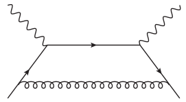
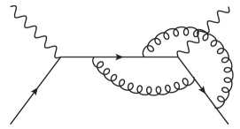
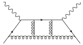
Figure 1: Sample Feynman diagrams for the scattering of an external current (wavy line) on a heavy quark (solid line). Taken from Ref. [14].

A constructive way to compute the HQET parameters in perturbation is given by the Small Velocity (SM) sum rules [11]. Here, one considers the scattering of a heavy quark $Q$ on a current $J$. The current transfers energy to the quark $Q$ and excites it, causing possibly emissions of further gluons or quarks. We denote the inclusive final state as $X_{Q}$. Working in the rest frame of the initial heavy quark we can define the excitation energy $\omega$ by

$$\omega =q_{0}-q_{0}^{\rm min}=q_{0}-\left(\sqrt{\vec{q}^{2}+m_{Q}^{2}}-m_{Q}\right)~{},$$ (3)

where $q=(q_{0},\vec{q})$ is the 4-momentum of the current. The velocity of the system $X_{Q}$ after the scattering is given by $\vec{v}=\vec{q}/m_{Q}$. The perturbative versions of the operator matrix elements can then be given by

$$[\overline{\Lambda}]_{\rm pert} =\lim\limits_{\vec{v}\to 0}\lim\limits_{m_{Q}\to\infty}\frac{2}{\vec{v}^{2}}\frac{\int_{0}^{\mu}\omega\,W(\omega,\vec{v})d\omega}{\int_{0}^{\mu}W(\omega,\vec{v})d\omega}~{},$$ (4)

$$[\mu_{\pi}^{2}]_{\rm pert} =\lim\limits_{\vec{v}\to 0}\lim\limits_{m_{Q}\to\infty}\frac{3}{\vec{v}^{2}}\frac{\int_{0}^{\mu}\omega^{2}\,W(\omega,\vec{v})d\omega}{\int_{0}^{\mu}W(\omega,\vec{v})d\omega}~{},$$ (5)

where $W(\omega,\vec{v})$ is the structure function corresponding to the scattering and the parameter $\mu$ is introduced as a Wilsonian cut-off in order to separate low and high energy effects. The perturbative versions of the operator matrix elements are therefore given by moments of the scattering cross section. However, the non-relativistic description in terms of excitation energy and velocity given in Eqs. (4) and (5) do not allow a straight forward expansion on the level of Feynman diagrams. For the calculation we followed the following strategy (see Ref. [14] for a more detailed discussion):

• We utilize the optical theorem and consider the discontinuity of the $bJ\to bJ$ forward scattering diagrams (see Figure 1 for example diagrams).

• We express the non-relativistic quantities $\omega$ and $\vec{v}^{2}$ in terms of the Lorentz invariants

  $$y=m_{Q}-s=-m_{Q}\omega(2+\vec{v}^{2})+\mathcal{O}(\omega^{2},\vec{v}^{4})~{},$$ (6)

  $$q^{2}=-m_{Q}\vec{v}^{2}(m_{Q}-\omega)+\mathcal{O}(\omega^{2},\vec{v}^{4})~{}.$$ (7)

• The limit $m_{Q}\to\infty$ can now be realized as the asymptotic expansion around the threshold $s=m_{Q}^{2}$ (or equivalently $y=0$) for which we use the strategy of expansion by region [17, 18]. The limit $\vec{v}\to 0$ can subsequently be realized by a naive Taylor expansion in $q$. When the leading terms in $y$ and $q^{2}$ of the structure function have been extracted we use Eqs. (6) and (7) to go back to the non-relativistic quantities and re-expand.

This strategy now allows to use the full machinery of multi-loop calculations, i.e. we generate one-, two- and three-loop forward scattering diagrams with qgraf [19] and use FORM [20] to insert the Feynman rules, perform the Dirac and color algebra and expand all loop-momenta according to the rules of asymptotic expansion. In the present case the momenta can either scale hard ($k_{i}\sim m_{b}$) or ultrasoft ($k_{i}\sim y/m_{b}$). The corresponding regions have been cross-checked with the program Asy.m [21]. After the expansion the denominators become linearly dependent, so a partial fraction decomposition becomes necessary. For this we used the program LIMIT [22], which automatizes this step. This program also maps each scalar integral to a unique integral family, so that we were able to reduce all integrals to a small set of master integrals using the programs FIRE [23] and LiteRed [24].

If the loop momenta in the asymptotic expansion scale hard ($k_{i}\sim m_{b}$), the master integrals are given by on-shell propagator integrals, which are well studied in the literature [25, 26, 27]. For ultrasoft momenta ($k_{i}\sim y/m_{b}$) new types of master integrals appear which were evaluated using Mellin-Barnes techniques and differential equations in auxillary parameters.

The final result is given by

$$\frac{m^{\text{kin}}}{m^{\text{OS}}} =1-\frac{\alpha_{s}^{(n_{l})}}{\pi}C_{F}\biggl{(}\frac{4}{3}\frac{\mu}{m^{\text{OS}}}+\frac{1}{2}\frac{\mu^{2}}{\left({m^{\text{OS}}}\right)^{2}}\biggr{)}+\left(\frac{\alpha_{s}^{(n_{l})}}{\pi}\right)^{2}C_{F}\Biggl{\{}\frac{\mu}{{m^{\text{OS}}}}\Biggl{[}C_{A}\biggl{(}-\frac{215}{27}+\frac{2\pi^{2}}{9}+\frac{22}{9}l_{\mu}\biggr{)}$$

$$\mbox{}+n_{l}T_{F}\biggl{(}\frac{64}{27}-\frac{8}{9}l_{\mu}\biggr{)}\Biggr{]}+\frac{\mu^{2}}{\left({m^{\text{OS}}}\right)^{2}}\Biggl{[}C_{A}\biggl{(}-\frac{91}{36}+\frac{\pi^{2}}{12}+\frac{11}{12}l_{\mu}\biggr{)}+n_{l}T_{F}\biggl{(}\frac{13}{18}-\frac{1}{3}l_{\mu}\biggr{)}\Biggr{]}\Biggr{\}}$$

$$\mbox{}+\left(\frac{\alpha_{s}^{(n_{l})}}{\pi}\right)^{3}C_{F}\Biggl{\{}\frac{\mu}{{m^{\text{OS}}}}\Biggl{[}C_{A}^{2}\biggl{(}-\frac{130867}{1944}+\frac{511\pi^{2}}{162}+\frac{19\zeta_{3}}{2}-\frac{\pi^{4}}{18}+\biggl{(}\frac{2518}{81}-\frac{22\pi^{2}}{27}\biggr{)}l_{\mu}-\frac{121}{27}l_{\mu}^{2}\biggr{)}$$

$$\mbox{}+C_{A}n_{l}T_{F}\biggl{(}\frac{19453}{486}-\frac{104\pi^{2}}{81}-2\zeta_{3}+\biggl{(}-\frac{1654}{81}+\frac{8\pi^{2}}{27}\biggr{)}l_{\mu}+\frac{88}{27}l_{\mu}^{2}\biggr{)}+C_{F}n_{l}T_{F}\biggl{(}\frac{11}{4}-\frac{4\zeta_{3}}{3}-\frac{2}{3}l_{\mu}\biggr{)}$$

$$\mbox{}+n_{l}^{2}T_{F}^{2}\biggl{(}-\frac{1292}{243}+\frac{8\pi^{2}}{81}+\frac{256}{81}l_{\mu}-\frac{16}{27}l_{\mu}^{2}\biggr{)}\Biggr{]}+\frac{\mu^{2}}{\left({m^{\text{OS}}}\right)^{2}}\Biggl{[}C_{A}^{2}\biggl{(}-\frac{96295}{5184}+\frac{445\pi^{2}}{432}+\frac{57\zeta_{3}}{16}-\frac{\pi^{4}}{48}$$

$$\mbox{}+\biggl{(}\frac{2155}{216}-\frac{11\pi^{2}}{36}\biggr{)}l_{\mu}-\frac{121}{72}l_{\mu}^{2}\biggr{)}+C_{A}n_{l}T_{F}\biggl{(}\frac{13699}{1296}-\frac{23\pi^{2}}{54}-\frac{3\zeta_{3}}{4}+\biggl{(}-\frac{695}{108}+\frac{\pi^{2}}{9}\biggr{)}l_{\mu}+\frac{11}{9}l_{\mu}^{2}\biggr{)}$$

$$\mbox{}+C_{F}n_{l}T_{F}\biggl{(}\frac{29}{32}-\frac{\zeta_{3}}{2}-\frac{1}{4}l_{\mu}\biggr{)}+n_{l}^{2}T_{F}^{2}\biggl{(}-\frac{209}{162}+\frac{\pi^{2}}{27}+\frac{26}{27}l_{\mu}-\frac{2}{9}l_{\mu}^{2}\biggr{)}\Biggr{]}\Biggr{\}}~{},$$ (8)

with $l_{\mu}=\ln\frac{2\mu}{\mu_{s}}$ ($\mu$ denotes the Wilsonian cutoff and $\mu_{s}$ the renormalization scale of the strong coupling constant) and the $SU(N_{c})$ color factors are given by $C_{F}=(N_{c}^{2}-1)/2N_{c}$, $C_{A}=N_{c}$ and $T_{F}=1/2$. Note that this relation takes into account finite charm quark mass effects. These effects are given by decoupling effects only, which we showed by explicit calculation. The conversion between the kinetic mass and other mass schemes has been included in the public programs RunDec [28] and REvolver [29].

3 The Semileptonic Decay Width to $\mathcal{O}(\alpha_{s}^{3})$

For the computation of the semileptonic decay width, we need to calculate the process

$$b(q)\to X_{c}(p_{x})\ell(p_{\ell})\overline{\nu}(p_{\nu}),$$ (9)

where $X_{c}$ is an inclusive state containing at least one charm quark and potentially other light quarks and gluons. We can again use the optical theorem and consider the imaginary parts of 5-loop forward scattering diagrams (see Figure 2).

Figure 2: Sample Feynman diagrams for calculation of the semileptonic decay rate at $\mathcal{O}(\alpha_{s}^{3})$. Straight, curly and dashed lines represent quarks, gluons and leptons, respectively. The weak interaction mediated by the $W$ boson is shown as a blob. Taken from Ref. [15].

Since a calculation with complete analytical dependence on the charm and bottom mass seems out of reach, we consider the diagrams in an asymptotic expansion around

$$\delta =1-\frac{m_{c}}{m_{b}}~{}.$$ (10)

Although the expansion parameter is large for physical values of $m_{c}$ and $m_{b}$ ($\delta\sim 0.7$), it has been shown in Ref.[30] at $\mathcal{O}(\alpha_{s}^{2})$ that this expansion converges well at the physical point and can even be extended down to $m_{c}\to 0$ ($\delta\to 1$) with reasonable precision. Furthermore, it turns out that in this limit the calculation simplifies:

• For the asymptotic expansion in the limit $\delta\to 0$ we can use expansion by regions. Here, the loop momenta can be either hard $k_{i}\sim m_{b}$ or ultrasoft $k_{i}\sim\delta m_{b}$ again.

• The leptonic momenta have to be ultrasoft in order to generate an imaginary part. This reduces the number of regions to be considered.

• In the $\delta$-expansion one can completely factorize the leptonic system and integrate it out without IBP reduction. We are therefore left with 3-loop integrals, although we started from 5-loop diagrams.

For the remaining 3-loop diagrams the scaling of the loop momenta can again either be hard or ultrasoft and the calculation can be performed in close analogy to the one of the kinetic mass relation discussed before. However, since we are not only interested in the leading term of the expansion in $\delta$ but aim for 8 terms in the expansion, we encounter huge intermediate expressions of $\mathcal{O}(100\,\text{GB})$ for individual diagrams and $\mathcal{O}(10^{7})$ scalar integrals with positive and negative indices up to 12 which needed to be reduced to master integrals. Furthermore, the wave function and mass renormalization constants at $\mathcal{O}(\alpha_{s}^{3})$ allowing for two massive quarks, where only a few term in the expansion $m_{c}\to 0$ had been known analytically before (see Ref. [31]), needed to be extended in order to renormalize the present calculation (see Ref. [32]).

Parametrizing the total decay rate as

$$\Gamma = \Gamma_{0}\left(X_{0}+C_{F}\sum\limits_{i=1}^{\infty}\left(\frac{\alpha_{s}}{\pi}\right)^{i}X_{i}\right)$$ (11)

we obtain the following contributions at $\mathcal{O}(\alpha_{s}^{3})$

$$X_{3} =\delta^{5}\biggl{(}\frac{266929}{810}-\frac{5248a_{4}}{27}+\frac{2186\pi^{2}\zeta_{3}}{45}-\frac{4094\zeta_{3}}{45}-\frac{1544\zeta_{5}}{9}-\frac{656l_{2}^{4}}{81}+\frac{1336}{405}\pi^{2}l_{2}^{2}+\frac{44888\pi^{2}l_{2}}{135}$$

$$\mbox{}-\frac{9944\pi^{4}}{2025}-\frac{608201\pi^{2}}{2430}\biggr{)}+\mathcal{O}(\delta^{6}).$$ (12)

We used the notations $l_{2}=\ln(2)$, $a_{4}=\text{Li}_{4}(1/2)$ and $\zeta_{i}$ is Riemanns zeta function. In the result above the color factors are specified to QCD and the renormalization scale $\mu_{s}=m_{b}$ has been chosen. The full result with general color factors and expanded up to $\mathcal{O}(\delta^{12})$ can be found in the ancillary file to Ref. [15]. Recently the results of a subset of color factors has been confirmed up to $\mathcal{O}(\delta^{9})$ in Ref. [33].

4 Phenomenological Results

Using the values $\alpha_{s}^{(5)}(M_{Z})=0.1179$ [34], $\overline{m}_{c}(3\,\text{GeV})=993~{}\text{MeV}$ [35] and $\overline{m}_{b}(\overline{m}_{b})=4163~{}\text{MeV}$ [36], we obtain

$$m_{b}^{\rm kin}(\mu=1\,\text{GeV}) =(4163+259+78+26\pm 13)\,\text{MeV}=(4526\pm 13)\,\text{MeV}~{}.$$ (13)

We estimate the error as half the $\mathcal{O}(\alpha_{s}^{3})$ correction, which is also consistent with the residual scale uncertainty and known contributions in the large $\beta_{0}$ approximation at 4-loop. The same approach at $\mathcal{O}(\alpha_{s}^{2})$ leads to an uncertainty of $39\,\text{MeV}$, the three-loop results therefore reduce the perturbative uncertainty by about a factor of two.

For the semileptonic decay rate in the on-shell scheme with $m_{b}^{\rm OS}=m_{b}=4.7\,\text{GeV}$ and $m_{c}^{\rm OS}=m_{c}=1.3\,\text{GeV}$ we obtain

$$\Gamma(m_{b},m_{c}) =\Gamma_{0}X_{0}\left[1-1.72\frac{\alpha_{s}^{(5)}}{\pi}-13.09\left(\frac{\alpha_{s}^{(5)}}{\pi}\right)^{2}-162.82\left(\frac{\alpha_{s}^{(5)}}{\pi}\right)^{3}\right]$$ (14)

One observes the expected bad convergence of the perturbative series. Using the kinetic scheme for the bottom quark and the $\overline{\text{MS}}$ scheme for the charm quark mass we obtain

$$\Gamma(m_{b}^{\rm kin},\overline{m}_{c}(3\,\text{GeV})) =\Gamma_{0}X_{0}\left[1-1.67\frac{\alpha_{s}^{(4)}}{\pi}-7.25\left(\frac{\alpha_{s}^{(4)}}{\pi}\right)^{2}-28.6\left(\frac{\alpha_{s}^{(4)}}{\pi}\right)^{3}\right]$$ (15)

Similar improvements in der perturbative behavior are also observed using other threshold mass schemes for the bottom quark mass. For a more detailed discussion see Ref. [15].

Both results have already been used to update the inclusive determination of $|V_{cb}|$ [5]. The inclusion of the presented $\mathcal{O}(\alpha_{s}^{3})$ corrections resulted in a small shift of the central value but reduced the uncertainty due to the semileptonic width $\Gamma$ by a factor of two.

References

- [1] C.W. Bauer, Z. Ligeti, M. Luke, A.V. Manohar and M. Trott, Global analysis of inclusive B decays, Phys. Rev. D 70 (2004) 094017 [hep-ph/0408002].
- [2] P. Gambino and C. Schwanda, Inclusive semileptonic fits, heavy quark masses, and , Phys. Rev. D 89 (2014) 014022 [1307.4551].
- [3] A. Alberti, P. Gambino, K.J. Healey and S. Nandi, Precision Determination of the Cabibbo-Kobayashi-Maskawa Element , Phys. Rev. Lett. 114 (2015) 061802 [1411.6560].
- [4] P. Gambino, K.J. Healey and S. Turczyk, Taming the higher power corrections in semileptonic B decays, Phys. Lett. B 763 (2016) 60 [1606.06174].
- [5] M. Bordone, B. Capdevila and P. Gambino, Three loop calculations and inclusive Vcb, Phys. Lett. B 822 (2021) 136679 [2107.00604].
- [6] M. Beneke and V.M. Braun, Heavy quark effective theory beyond perturbation theory: Renormalons, the pole mass and the residual mass term, Nucl. Phys. B 426 (1994) 301 [hep-ph/9402364].
- [7] I.I.Y. Bigi, M.A. Shifman, N.G. Uraltsev and A.I. Vainshtein, The Pole mass of the heavy quark. Perturbation theory and beyond, Phys. Rev. D 50 (1994) 2234 [hep-ph/9402360].
- [8] A.H. Hoang, Z. Ligeti and A.V. Manohar, B decay and the Upsilon mass, Phys. Rev. Lett. 82 (1999) 277 [hep-ph/9809423].
- [9] A.H. Hoang, Z. Ligeti and A.V. Manohar, B decays in the upsilon expansion, Phys. Rev. D 59 (1999) 074017 [hep-ph/9811239].
- [10] A.H. Hoang and A.V. Manohar, Charm effects in the MS-bar bottom quark mass from Upsilon mesons, Phys. Lett. B 483 (2000) 94 [hep-ph/9911461].
- [11] I.I.Y. Bigi, M.A. Shifman, N.G. Uraltsev and A.I. Vainshtein, Sum rules for heavy flavor transitions in the SV limit, Phys. Rev. D 52 (1995) 196 [hep-ph/9405410].
- [12] I.I.Y. Bigi, M.A. Shifman, N. Uraltsev and A.I. Vainshtein, High power n of m(b) in beauty widths and n=5 — infinity limit, Phys. Rev. D 56 (1997) 4017 [hep-ph/9704245].
- [13] M. Fael, K. Schönwald and M. Steinhauser, Kinetic Heavy Quark Mass to Three Loops, Phys. Rev. Lett. 125 (2020) 052003 [2005.06487].
- [14] M. Fael, K. Schönwald and M. Steinhauser, Relation between the and the kinetic mass of heavy quarks, Phys. Rev. D 103 (2021) 014005 [2011.11655].
- [15] M. Fael, K. Schönwald and M. Steinhauser, Third order corrections to the semileptonic b→c and the muon decays, Phys. Rev. D 104 (2021) 016003 [2011.13654].
- [16] A. Czarnecki, K. Melnikov and N. Uraltsev, NonAbelian dipole radiation and the heavy quark expansion, Phys. Rev. Lett. 80 (1998) 3189 [hep-ph/9708372].
- [17] M. Beneke and V.A. Smirnov, Asymptotic expansion of Feynman integrals near threshold, Nucl. Phys. B 522 (1998) 321 [hep-ph/9711391].
- [18] V.A. Smirnov, Analytic tools for Feynman integrals, vol. 250, Springer (2012), 10.1007/978-3-642-34886-0.
- [19] P. Nogueira, Automatic Feynman graph generation, J. Comput. Phys. 105 (1993) 279.
- [20] B. Ruijl, T. Ueda and J. Vermaseren, FORM version 4.2, 1707.06453.
- [21] B. Jantzen, A.V. Smirnov and V.A. Smirnov, Expansion by regions: revealing potential and Glauber regions automatically, Eur. Phys. J. C 72 (2012) 2139 [1206.0546].
- [22] F. Herren, Precision Calculations for Higgs Boson Physics at the LHC - Four-Loop Corrections to Gluon-Fusion Processes and Higgs Boson Pair-Production at NNLO, Ph.D. thesis, KIT, Karlsruhe, 2020. 10.5445/IR/1000125521.
- [23] A.V. Smirnov and F.S. Chuharev, FIRE6: Feynman Integral REduction with Modular Arithmetic, Comput. Phys. Commun. 247 (2020) 106877 [1901.07808].
- [24] R.N. Lee, LiteRed 1.4: a powerful tool for reduction of multiloop integrals, J. Phys. Conf. Ser. 523 (2014) 012059 [1310.1145].
- [25] S. Laporta and E. Remiddi, The Analytical value of the electron (g-2) at order alpha**3 in QED, Phys. Lett. B 379 (1996) 283 [hep-ph/9602417].
- [26] K. Melnikov and T. van Ritbergen, The Three loop on-shell renormalization of QCD and QED, Nucl. Phys. B 591 (2000) 515 [hep-ph/0005131].
- [27] R.N. Lee and V.A. Smirnov, Analytic Epsilon Expansions of Master Integrals Corresponding to Massless Three-Loop Form Factors and Three-Loop g-2 up to Four-Loop Transcendentality Weight, JHEP 02 (2011) 102 [1010.1334].
- [28] F. Herren and M. Steinhauser, Version 3 of RunDec and CRunDec, Comput. Phys. Commun. 224 (2018) 333 [1703.03751].
- [29] A.H. Hoang, C. Lepenik and V. Mateu, REvolver: Automated running and matching of couplings and masses in QCD, Comput. Phys. Commun. 270 (2022) 108145 [2102.01085].
- [30] M. Dowling, J.H. Piclum and A. Czarnecki, Semileptonic decays in the limit of a heavy daughter quark, Phys. Rev. D 78 (2008) 074024 [0810.0543].
- [31] S. Bekavac, A. Grozin, D. Seidel and M. Steinhauser, Light quark mass effects in the on-shell renormalization constants, JHEP 10 (2007) 006 [0708.1729].
- [32] M. Fael, K. Schönwald and M. Steinhauser, Exact results for and with two mass scales and up to three loops, JHEP 10 (2020) 087 [2008.01102].
- [33] M. Czakon, A. Czarnecki and M. Dowling, Three-loop corrections to the muon and heavy quark decay rates, Phys. Rev. D 103 (2021) L111301 [2104.05804].
- [34] Particle Data Group collaboration, Review of Particle Physics, PTEP 2020 (2020) 083C01.
- [35] K.G. Chetyrkin, J.H. Kuhn, A. Maier, P. Maierhofer, P. Marquard, M. Steinhauser et al., Addendum to “Charm and bottom quark masses: An update”, 1710.04249.
- [36] K.G. Chetyrkin, J.H. Kuhn, A. Maier, P. Maierhofer, P. Marquard, M. Steinhauser et al., Charm and Bottom Quark Masses: An Update, Phys. Rev. D 80 (2009) 074010 [0907.2110].