Elevated Hot Gas and High-Mass X-ray Binary Emission in Low Metallicity Galaxies: Implications for Nebular Ionization and Intergalactic Medium Heating in the Early Universe

Abstract

High-energy emission associated with star formation has been proposed as a significant source of interstellar medium (ISM) ionization in low-metallicity starbursts and an important contributor to the heating of the intergalactic medium (IGM) in the high-redshift ($z\lower 2.15277pt\hbox{$\;\buildrel>\over{\sim}\;$}8$) Universe. Using Chandra observations of a sample of 30 galaxies at $D\approx$ 200–450 Mpc that have high specific star-formation rates of 3–9 Gyr^-1 and metallicities near $Z\approx 0.3Z_{\_}\odot$, we provide new measurements of the average 0.5–8 keV spectral shape and normalization per unit star-formation rate (SFR). We model the sample-combined X-ray spectrum as a combination of hot gas and high-mass X-ray binary (HMXB) populations and constrain their relative contributions. We derive scaling relations of $\log L_{\_}{\rm 0.5-8keV}^{\rm HMXB}$/SFR $=40.19\pm 0.06$ and $\log L_{\_}{\rm 0.5-2keV}^{\rm gas}$/SFR $=39.58^{+0.17}_{\_}{-0.28}$; significantly elevated compared to local relations. The HMXB scaling is also somewhat higher than $L_{\_}{\rm 0.5-8keV}^{\rm HMXB}$-SFR-$Z$ relations presented in the literature, potentially due to our galaxies having relatively low HMXB obscuration and young and X-ray luminous stellar populations. The elevation of the hot gas scaling relation is at the level expected for diminished attenuation due to a reduction of metals; however, we cannot conclude that an $L_{\_}{\rm 0.5-2keV}^{\rm gas}$-SFR-$Z$ relation is driven solely by changes in ISM metal content. Finally, we present SFR-scaled spectral models (both emergent and intrinsic) that span the X-ray–to–IR band, providing new benchmarks for studies of the impact of ISM ionization and IGM heating in the early Universe.

1 Introduction

The X-ray power output from normal galaxies (i.e., galaxies that do not harbor luminous active galactic nuclei [AGN]) is dominated by diffuse hot gas and X-ray binaries (XRBs), with additional minor contributions from supernovae and their remnants (see, e.g., Fabbiano, 1989, 2006, 2019, for reviews). The Chandra X-ray Observatory (hereafter, Chandra) has provided resolved views of the X-ray emission on subgalactic scales for 100s of relatively nearby ($D<30$ Mpc) galaxies, and XMM-Newton has provided unprecedented spectral constraints and physical insight into the emission from several of these objects.

For star-forming normal galaxies, it has been shown that the galaxy-wide X-ray power output, $L_{\_}{\rm X}$, scales linearly with star-formation rate (hereafter, $L_{\_}{\rm X}$-SFR relations; see, e.g., Ranalli et al., 2003; Persic & Rephaeli, 2007; Lehmer et al., 2008, 2010; Basu-Zych et al., 2013a; Mineo et al., 2014; Symeonidis et al., 2014; Kouroumpatzakis et al., 2020). More detailed investigations of galaxy components (both from spatial and spectral analyses) reveal separate linear $L_{\_}{\rm X}$-SFR relations for diffuse hot gas (e.g., Strickland & Stevens, 2000; Tyler et al., 2004; Li & Wang, 2013a; Mineo et al., 2012a) and high-mass XRBs (HMXBs) (e.g., Grimm et al., 2003; Mineo et al., 2012b; Lehmer et al., 2019). However, the levels of statistical fluctuations in these relations is larger than that expected from photometric scatter, suggesting that additional physical variations, beyond SFR, influence $L_{\_}{\rm X}$.

With the advent of computationally intensive XRB population synthesis models (e.g., Fragos et al., 2008, 2013b, 2013a; Linden et al., 2010; Madau & Fragos, 2017; Wiktorowicz et al., 2017), it has become clear that the $L_{\_}{\rm X}$-SFR relation for HMXBs should not be universal, and should have additional non-negligible dependencies on star-formation history and metallicity. Metallicity, in particular, is expected to have a significant impact on the local $L_{\_}{\rm X}$-SFR relation and its scatter, given the breadth of galaxy metallicities present in local-galaxy samples. Low metallicity stellar populations are expected to have relatively weak mass loss from stellar winds, resulting in less angular momentum loss from binary systems, less binary widening over stellar evolutionary timescales, and more numerous and massive compact objects. These ingredients are predicted to result in an anticorrelation between $L_{\_}{\rm X}$/SFR and metallicity.

One of the key predictions by the Fragos et al. (2013b) XRB population synthesis model is that the typical $L_{\_}{\rm X}$(HMXB)/SFR ratio for galaxies in the Universe should rise with increasing redshift, due to the corresponding decline in galaxy-average metallicity. Using stacking analyses in the Chandra Deep Field-South, Lehmer et al. (2016) showed that there is indeed observable redshift evolution in the $L_{\_}{\rm X}$/SFR relation across the redshift range $z\approx$ 0–2, such that $L_{\_}{\rm X}$/SFR $\propto(1+z)$, consistent with some of the most viable models from Fragos et al. (2013b). Additional investigations have since reached consistent conclusions out to $z\approx$ 6 (e.g., Vito et al., 2016; Aird et al., 2017; Saxena et al., 2021). Studies of local galaxies have further corroborated the connection between HMXB population formation and metallicity, showing unambiguously that $L_{\_}{\rm X}$(HMXB)/SFR increases with decreasing metallicity ($Z$), in a claimed $L_{\_}{\rm X}$(HMXB)-SFR-$Z$ plane (see, e.g., Basu-Zych et al., 2013b, 2016; Prestwich et al., 2013; Douna et al., 2015; Brorby et al., 2016; Kovlakas et al., 2020; Lehmer et al., 2021; Vulic et al., 2021). Recently, Fornasini et al. (2019, 2020) showed more directly that $z\approx$ 0.1–2.6 galaxies with spectroscopically constrained metallicities fall onto the $L_{\_}{\rm X}$(HMXB)-SFR-$Z$ plane and can explain the observed redshift evolution.

The recently established connection between the $L_{\_}{\rm X}$(HMXB)-SFR relation and metallicity has led to a surge in interest in HMXBs as potentially important sources of ionizing radiation in low-metallicity galaxies, and several observations have found enhanced X-ray emission in galaxies selected by extreme ionization signatures, including Ly$\alpha$ and He II emitters, green peas, and Lyman-continuum galaxies (see, e.g., Brorby & Kaaret, 2017; Bluem et al., 2019; Svoboda et al., 2019; Bayliss et al., 2020; Dittenber et al., 2020; Gross et al., 2021). Notably, X-ray emission (particularly from HMXBs) has been implicated as a potential solution to the long-standing problem of how nebular He II is produced in low-metallicity star-forming galaxies (see, e.g., Pakull & Angebault, 1986; Schaerer, 1996; Shirazi & Brinchmann, 2012; Jaskot & Oey, 2013; Crowther et al., 2016; Senchyna et al., 2019; Berg et al., 2021; Olivier et al., 2021, for discussions of He II production in galaxies); however, uncertainties in the extrapolations of the intrinsic spectral energy distribution (SED) into the EUV (near the He II ionization energy of 54 eV) has resulted in the connection between He II and X-ray emission being a topic of active debate (e.g., Schaerer et al., 2019; Senchyna et al., 2020; Saxena et al., 2020; Kehrig et al., 2021; Rickards Vaught et al., 2021; Simmonds et al., 2021).

In addition to the X-ray/extreme-ionization connection, the metallicity-dependent $L_{\_}{\rm X}$-SFR relation has been actively studied for its role in heating the intergalactic medium (IGM) in the early Universe. Extrapolation of the most viable Fragos et al. (2013a) $L_{\_}{\rm X}$(HMXB)/SFR models to redshifts beyond those constrained by Lehmer et al. (2016, $z\approx$ 0–2) suggests that HMXBs would have dominated the X-ray emissivity of the $z\lower 2.15277pt\hbox{$\;\buildrel>\over{\sim}\;$}$8 Universe, surpassing the contributions from AGN. X-ray emission from HMXBs is promising as a source of IGM heating, since the emission both persists on timescales longer than that of ionizing far-UV emission from young massive stars and traverses longer path lengths before being absorbed (e.g., Mirabel et al., 2011; Madau & Fragos, 2017). Cosmological simulations that track the spin temperature evolution of the very early Universe ($z\lower 2.15277pt\hbox{$\;\buildrel>\over{\sim}\;$}10$) have implicated X-ray emission as potentially the main source of heating the neutral IGM, prior to reionization (see, e.g., Mesinger et al., 2013; Pacucci et al., 2014; Park et al., 2019; Eide et al., 2020; Heneka & Mesinger, 2020). However, similar to studies of He II, the impact of X-ray heating depends upon knowledge of the X-ray spectrum at low energies; in this case, the emergent X-ray spectrum at $E\lower 2.15277pt\hbox{$\;\buildrel<\over{\sim}\;$}1$ keV is of critical importance (e.g., Pacucci et al., 2014; Das et al., 2017).

As discussed above, the impact of X-ray emitting components as sources of ionization and high-redshift IGM heating depend critically on knowledge of the intrinsic and emergent SEDs from low-metallicity galaxies. Thus far, constraints on low-metallicity galaxy X-ray spectra are based on either small numbers of objects (e.g., Thuan et al., 2004; Lehmer et al., 2015; Garofali et al., 2020) or shallow observations of relatively nearby dwarf galaxies (Prestwich et al., 2013; Douna et al., 2015), which are subject to very large statistical scatter in their HMXB luminosity scaling with SFR (see, e.g., Lehmer et al., 2021). Nonetheless, from these observations, Garofali et al. (2020) showed that the low-metallicity star-forming galaxies NGC 3310 and VV114 exhibit enhanced power output per SFR relative to nearly solar-metallicity galaxies, across the full 0.3–30 keV spectral range, motivating future studies of larger galaxy populations.

Here we provide a new benchmark characterizing how the average X-ray spectra of star-forming galaxies scales with SFR for a sample of galaxies selected to have characteristics in common with high-redshift galaxies (e.g., low-metallicity and evidence of active star formation from young stellar populations). We present Chandra observations for a sample of 30 relatively nearby star-forming-active galaxies, with $12+\log({\rm O}/{\rm H})$ $\approx$ 8.1–8.2 ($Z\approx$ 0.3 $Z_{\_}\odot$), SFR $\approx$ 0.5–15 $M_{\odot}$ yr^-1, and $\log M_{\_}\star/M_{\_}\odot\approx$ 8–9.3. Our sample size and high SFR values allow us to provide statistically meaningful constraints on the population-average 0.5–8 keV SED and its statistical scatter.

In §2, we describe the selection of our low-metallicity galaxy sample. In §3, we describe our multiwavelength FUV to mid-IR SED fitting and present derived physical properties for our galaxy sample. In §4, we describe our new Chandra observations, and discuss our data reduction and X-ray spectral modeling procedure. In §5, we show modeling of the average X-ray spectrum scaling with SFR for our sample, disentangle and constrain HMXB and hot gas contributions to the overall spectral shape, and investigate the spectra of individual galaxies. In §6, we study the $L_{\_}{\rm X}$/SFR relation, its statistical scatter, and its dependence on metallicity for both HMXBs and hot gas. We further present new constraints and extrapolations of the emergent and intrinsic average SED of the population, spanning the mid-IR to X-rays. Finally, in §7, we summarize the key results of the paper.

Throughout this paper, we make reference to X-ray fluxes that have been corrected for Galactic absorption, but not intrinsic absorption. Similarly, X-ray luminosities are always reported as “observed” quantities that are not corrected for intrinsic absorption; however, our presentation of intrinsic X-ray spectra contain corrections for intrinsic absorption as described in the text. For comparisons with past studies, we make use of a Kroupa (2001) initial mass function (IMF) when deriving physical properties from multiwavelength UV–to–IR SED fitting, and we utilize a $\Lambda$CDM cosmology, with values of $H_{\_}0$ = 70 km s^-1 Mpc^-1, $\Omega_{\_}{\rm M}$ = 0.3, and $\Omega_{\_}{\Lambda}$ = 0.7 adopted (e.g., Spergel et al., 2003).

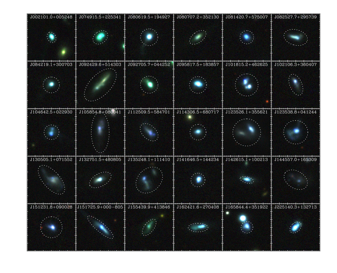
Figure 1: PanSTARRS three-band images ($g$ = blue, $i$ = green, and $z$ = red) for the 30 galaxies in our sample. Each image is 30 $\times$ 30 arcsec² in extent. The dotted circular or elliptical regions indicate the regions used to extract X-ray source counts; the parameters of these regions (i.e., central locations, major and minor axes, and position angles) are specified in Table 1.

2 Sample Selection

Our goal was to select a statistically meaningful sample of galaxies that would allow us to accurately characterize the SFR-scaled X-ray emission in the low-metallicity regime. Such a characterization is critical for developing a fundamental understanding of the X-ray heating of the IGM by the first galaxies and the ionizing emission from X-ray sources in low-metallicity galaxies. We started by using the starlight-subtracted emission-line fluxes published in the SDSS DR7 MPA-JHU value added catalogs to identify potential AGN and calculate metallicities for a sample of galaxies that had H$\alpha$, H$\beta$, O III, and N II emission-line fluxes detected at the $>$3$\sigma$ level. We removed objects that were clearly AGN, based on BPT diagnostics; however, we recognize that obscured or low-luminosity AGN may still remain, and we revisit potential AGN in our sample based on X-ray characteristics in § 5.2. For the remaining galaxies, we used the “PP04 O3N2” method (Pettini & Pagel, 2004, hereafter, PP04) to convert strong emission-line flux ratios into metallicities. This method uses an empirical calibration of the OIII]/[H$\beta$]–to–[NII]/[H$\alpha$] emission-line ratio versus metallicity for $>$100 H II regions. The conversion has been shown to provide accurate gas-phase metallicities for galaxies with $12+\log({\rm O}/{\rm H})$ $>8.09$ (or $Z\lower 2.15277pt\hbox{$\;\buildrel>\over{\sim}\;$}0.25Z_{\_}\odot$), and it provides one of the most robust metallicity diagnostics and avoids introducing additional scatter (up to 0.7 dex) from applying different metallicity methods (e.g. Kewley & Ellison, 2008). Furthermore, this metallicity calibration allows for direct comparisons with the Lehmer et al. (2021, hereafter, L21) study of the metallicity-depdendent HMXB X-ray luminosity function scaling relation, which is also based on the PP04 calibration. L21 provides the most up-to-date $L_{\_}{\rm X}$(HMXB)-SFR-$Z$ relation and quantifies the SFR-dependent scatter of the relation.

For sample selection purposes, we selected all galaxies with metallicities in the narrow range of $12+\log({\rm O}/{\rm H})$ $=$ 8.1–8.2 ($Z\approx 0.26$–0.32 $Z_{\_}\odot$), near the lowest limit by which the PP04 diagnostic is accurate. For context, e.g., Madau & Fragos (2017, see their Fig. 2) and Guo et al. (2010) show that a metallicity of $Z\approx 0.3Z_{\_}\odot$ corresponds to the mass-weighted metallicity of the Universe at $z\approx 6$ and the metallicity of relatively massive galaxies $\log M_{\_}\star/M_{\_}\odot\approx$ 9–10 at $z\approx 10$, where the knee of the stellar mass function is estimated to be $\mathcal{M}_{\_}\star^{*}\approx 10^{9.5}$ $M_{\odot}$ (e.g., Stefanon et al., 2021). To further identify galaxies that were more explicitly similar to $z\approx 10$ massive galaxies, we made use of the SFR and $M_{\_}\star$ estimates from Salim et al. (2016), and filtered our sample to contain galaxies with SFR $\approx$ 2–20 $M_{\odot}$ yr^-1 and $\log M_{\_}\star/M_{\_}\odot\approx$ 8.5–10 (see, e.g., Guo et al., 2010; Salmon et al., 2015; Song et al., 2016). We note that the properties of these galaxies will not precisely match $z\approx 10$ galaxies in morphology, stellar density, and star-formation history; however, the three properties of selection used here (i.e., metallicity, SFR, and $M_{\_}\star$) are expected to be among the most important for XRB formation (e.g., Fragos et al., 2013b, a; Wiktorowicz et al., 2017) and can lead to new insight regarding the X-ray emission from such galaxy populations.

To optimize our sample for observation, we sorted our initial sample by the quantity SFR/$d_{\_}L^{2}$, which is a proxy for the X-ray brightness of a given galaxy. We performed simulations to assess how galaxy-to-galaxy scatter influence the overall average spectral shape and found that constraints based on a sample of the first 30 galaxies in our sample would give a robust measurement of the galaxy-population averaged spectrum and SFR scaling with minimal impact from statistical scatter. We therefore selected the first 30 galaxies in the sample for observation with Chandra. The full sample of 30 galaxies was observed by Chandra through the combination of archival observations for three galaxies (J002101.0+005248.1, J080619.5+194927.3, and J225140.3+132713.4; see Basu-Zych et al., 2013b) and new observations of the remaining 27 objects (PI: Lehmer). In Table 1, we list the galaxies in our sample in order of right ascension (R.A.), and in Figure 1, we show corresponding Pan-STARRS $giz$ (blue, green, red) image cutouts. These cutouts illustrate that galaxies in our sample have blue optical colors, clearly indicative of active star formation, and have irregular and complex morphological types, many of which indicate interacting systems. These properties are similar to those of Lyman break analogs (LBAs), which have been the focus of other X-ray studies of high-redshift analogs (see, e.g., Basu-Zych et al., 2013b; Brorby et al., 2016).

3 Galaxy Physical Properties

Given the morphological variety and multiple components that are apparent for some of our galaxies, we chose to perform our own detailed photometric extraction and SED fitting of the available FUV-to-mid-IR data to derive physical properties. We made use of the Lightning SED fitting code (see Eufrasio et al., 2017), which fits broadband SEDs using a non-parametric star-formation history (SFH) model, including prescriptions for attenuation and nebular and dust emission (see Doore et al., 2021, for further details). A detailed account of the SED fitting of this sample and its results will be presented in a forthcoming paper (Eufrasio et al. in-prep); however, for completeness, we describe the salient details and results below.

We extracted broadband photometry from GALEX (Morrissey et al., 2007), SDSS (Alam et al., 2015), PanSTARRS (Chambers et al., 2016; Waters et al., 2020), 2MASS (2MASS Team, 2020), and WISE (WISE Team, 2020) for all galaxies, providing SED constraints from 0.15–22$\mu$m. For all galaxies, we specified either circular or elliptical galactic regions by visual analysis of the PanSTARRS $g$-band images. The central positions and dimensions of these regions are provided in Table 1 as Col.(2)–(3) and Col.(6)–(8), respectively, and they are overlaid in Figure 1. For a given bandbass, we extracted on-source photometry using expanded versions of these regions, which consisted of the galactic regions plus four times the half-width at half max PSF appropriate for the bandpass. In this process, we subtracted emission from unrelated nearby Galactic stars (J165844.4+351922) following the procedures in Eufrasio et al. (2017). Galactic stars can contribute non-negligible emission in bandpasses at wavelengths shortward of the WISE bands. Furthermore, in the case of J105854.8+080041, we found that the relatively large PSF of WISE permitted significant contributions from a nearby unrelated galaxy in the WISE bands that dominated over the target source. Since these contributions were inseparable, we chose to model this SED excluding the WISE data.

Local backgrounds for all bands were estimated using annuli that were located 2–4 times the expanded regions that were used for on-source photometry. Within these regions, we adopted the mode of the background distribution of the pixels as the local background level. This local background was appropriately rescaled and subtracted from the on-source photometry.

Using the background-subtracted 0.15–22$\mu$m photometry, we fit each galaxy SED with Lightning using a SFH model that consisted of five discrete time steps, of constant SFR, at 0–10 Myr, 10–100 Myr, 0.1–1 Gyr, 1–5 Gyr, and 5–13.6 Gyr. The SFH model specifies the intrinsic stellar and nebular spectral shape, which is further modified by attenuation by dust and re-emission of the absorbed radiation in the infrared. We modeled the attenuation using a three-parameter, modified Calzetti et al. (2000) extinction curve (as described in Eufrasio et al., 2017), and dust emission was modeled using Draine & Li (2007) models (with the five-parameter implementation described in Doore et al., 2021).

For each galaxy, we used the derived SFHs to calculate SFR and $M_{\_}\star$ values following:

$${\rm SFR}=\frac{1}{100~{}{\rm Myr}}\int_{\_}0^{\rm 100~{}Myr}\psi(t)\;dt,$$ (1)

and

$$M_{\_}\star=\int_{\_}0^{\rm 13.6~{}Gyr}R(t)\;\psi(t)\;dt,$$ (2)

where $t$ represents the look-back time and $\psi(t)$ represents the instantaneous SFR at look-back time $t$ (e.g., $\psi(0)$ is the instantaneous SFR at the present day), and $R(t)$ converts the mass of stars formed in the interval between $t$ and $t+dt$ to its contribution to the present-day stellar mass at $t=0$. In Eqn. 1 (and hereafter), SFR is defined as the mean value of $\psi(t)$ over the last 100 Myr; this definition is compatible with those used for widely-used scaling relations that convert intrinsic UV luminosity to SFR (e.g., Kennicutt, 1998; Hao et al., 2011).

In Figure 2, we show the SFR versus $M_{\_}\star$ and specific-SFR (sSFR $\equiv$ SFR/$M_{\_}\star$) versus metallicity for galaxies in our sample. By construction, based on the properties presented in Salim et al. (2016) (see § 2), the range of parameters span the area of SFR $\approx$ 0.5–15 $M_{\odot}$ yr^-1, $\log M_{\_}\star/M_{\_}\odot=$ 8.0–9.3, and $12+\log({\rm O}/{\rm H})$ $=$ 8.1–8.2. Figure 2 also shows the properties of relevant comparison samples that have been used to place constraints on X-ray scaling relations among star-forming galaxies. These samples include (1) five local galaxies with excellent global X-ray spectral constraints from Lehmer et al. (2015) and Garofali et al. (2020) (NGC 3310, NGC 253, NGC 3256, M83, VV114); (2) the 33 star-forming galaxies presented in the main sample of L21, who characterized how the HMXB X-ray luminosity function (XLF) and $L_{\_}{\rm X}$(HMXB)/SFR scaling varies with metallicity; (3) stacked galaxy subsamples of $z=$ 0.1–2.6 galaxies in the COSMOS and Chandra Deep Field-South (CDF-S) surveys that have been used to directly constrain the $L_{\_}{\rm X}$-SFR-$Z$ relation for large galaxy samples (Fornasini et al., 2019, 2020); and (4) three green pea galaxies with high SFRs that have been studied in X-rays by Svoboda et al. (2019).

Our sample appears to have SFR, $M_{\_}\star$, and metallicity values that overlap NGC 3310, and has very high sSFR values of 3–9 Gyr^-1, comparable to green peas and extreme emission line galaxies at $z\approx$ 7–9 that have intense UV emission from very young stellar populations (e.g., Mainali et al., 2017, 2018; Stark et al., 2017). As such, we expect that our galaxies host stellar populations that are young relative to our comparison samples, which span a broader sSFR range.

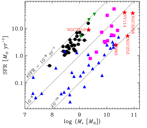
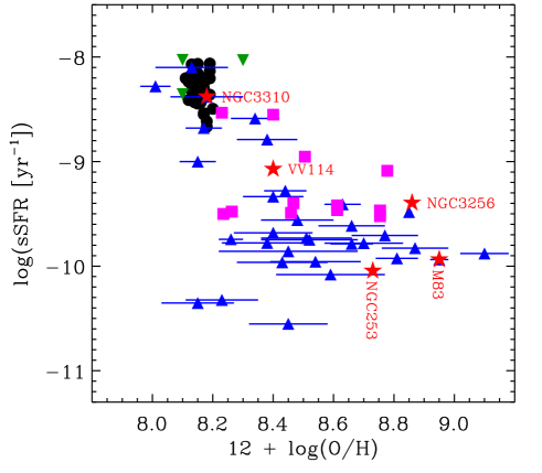
Figure 2: ($a$) SFR versus logarithm of the stellar mass for the 30 galaxies in our sample (black circles) and comparison samples from (1) five well-studied galaxies with spectral constraints across the 0.3–30 keV band from Garofali et al. (2020, red stars with annotated labels); (2) the main sample of nearby ($D<30$ Mpc) star-forming galaxies from L21 (blue triangles); (3) three “green pea” galaxies with relatively high SFR that were classified as star-forming galaxies (Svoboda et al., 2019, green downward triangles); (4) the Chandra stacked samples from Fornasini et al. (2019, 2020, magenta squares). ($b$) Logarithm of the specific-SFR (sSFR = SFR/$M_{\_}\star$) versus gas-phase metallicity ($12+\log({\rm O}/{\rm H})$) for our sample and the comparison samples.

Table 1: Galaxy Sample Properties

					Size Parameters
Galaxy	Central Position		$N_{\_}{\rm H,gal}$	$D$	$a$	$b$	PA	$\log M_{\_}\star$	SFR	$12+\log({\rm O/H})$
Name	$\alpha_{\_}{\rm J2000}$	$\delta_{\_}{\rm J2000}$	(1020 cm-2)	(Mpc)	(arcsec)		(deg)	($M_{\_}\odot$)	($M_{\odot}$ yr-1)	(dex)
(1)	(2)	(3)	(4)	(5)	(6)	(7)	(8)	(9)	(10)	(11)
J002101.0+005248.1	00 21 01.0	+00 52 48.0	2.62	452.4	3.47	2.59	26	9.32${}^{+0.06}_{\_}{-0.07}$	15.32${}^{+0.82}_{\_}{-0.67}$	8.19
J074915.5+225342.2	07 49 15.5	+22 53 41.9	4.95	203.0	5.03	3.69	128	8.62${}^{+0.07}_{\_}{-0.06}$	1.77${}^{+0.10}_{\_}{-0.10}$	8.18
J080619.5+194927.3	08 06 19.5	+19 49 27.3	3.44	314.6	5.29	…	…	9.01${}^{+0.06}_{\_}{-0.05}$	7.10${}^{+0.36}_{\_}{-0.36}$	8.15
J080707.2+352130.3	08 07 07.2	+35 21 30.3	4.98	280.4	5.85	3.24	127	8.84${}^{+0.11}_{\_}{-0.11}$	1.48${}^{+0.13}_{\_}{-0.17}$	8.18
J081420.8+575008.0	08 14 20.7	+57 50 08.0	4.38	246.6	4.19	…	…	8.53${}^{+0.09}_{\_}{-0.10}$	1.42${}^{+0.12}_{\_}{-0.14}$	8.16
J082527.7+295739.3	08 25 27.7	+29 57 39.8	3.83	223.5	7.39	4.86	254	8.60${}^{+0.09}_{\_}{-0.10}$	1.28${}^{+0.11}_{\_}{-0.11}$	8.20
J084219.1+300703.6	08 42 19.1	+30 07 03.4	4.15	382.8	5.03	…	…	9.18${}^{+0.10}_{\_}{-0.10}$	3.66${}^{+0.35}_{\_}{-0.48}$	8.18
J092429.9+514301.2	09 24 29.6	+51 43 03.2	1.45	214.0	12.66	6.46	137	8.53${}^{+0.09}_{\_}{-0.11}$	1.24${}^{+0.14}_{\_}{-0.16}$	8.14
J092705.7+044251.9	09 27 05.7	+04 42 52.0	3.69	272.4	5.37	…	…	8.95${}^{+0.07}_{\_}{-0.07}$	2.61${}^{+0.14}_{\_}{-0.18}$	8.17
J095817.5+183858.1	09 58 17.5	+18 38 57.8	2.98	278.1	5.26	…	…	8.90${}^{+0.08}_{\_}{-0.07}$	5.11${}^{+0.30}_{\_}{-0.29}$	8.18
J101815.1+462623.9	10 18 15.2	+46 26 25.2	0.99	364.6	6.99	…	…	9.09${}^{+0.12}_{\_}{-0.12}$	5.74${}^{+0.61}_{\_}{-0.42}$	8.15
J102106.4+360408.8	10 21 06.3	+36 04 07.1	1.27	335.2	7.01	3.69	22	8.77${}^{+0.09}_{\_}{-0.11}$	2.42${}^{+0.14}_{\_}{-0.19}$	8.16
J104642.5+022930.0	10 46 42.5	+02 29 30.7	3.82	396.4	4.58	…	…	8.68${}^{+0.07}_{\_}{-0.08}$	2.98${}^{+0.10}_{\_}{-0.11}$	8.19
J105854.8+080044.1	10 46 42.5	+02 29 30.7	2.95	226.5	12.87	5.49	0	8.44${}^{+0.12}_{\_}{-0.14}$	1.37${}^{+0.12}_{\_}{-0.12}$	8.15
J112509.5+584700.8	11 25 09.5	+58 47 01.3	0.91	272.2	6.59	4.14	45	8.41${}^{+0.07}_{\_}{-0.07}$	1.44${}^{+0.11}_{\_}{-0.11}$	8.17
J114306.5+680717.8	11 43 06.5	+68 07 17.5	1.44	217.3	4.95	…	…	8.53${}^{+0.09}_{\_}{-0.12}$	2.11${}^{+0.29}_{\_}{-0.22}$	8.14
J123525.9+355622.9	12 35 26.1	+35 56 21.0	1.37	187.6	8.57	…	…	8.59${}^{+0.09}_{\_}{-0.09}$	2.01${}^{+0.16}_{\_}{-0.15}$	8.17
J123538.7+041244.8	12 35 38.8	+04 12 44.4	1.85	328.3	7.43	…	…	8.83${}^{+0.10}_{\_}{-0.10}$	3.96${}^{+0.23}_{\_}{-0.25}$	8.12
J130505.1+071552.0	13 05 05.1	+07 15 52.4	2.13	277.1	11.07	5.19	40	8.72${}^{+0.08}_{\_}{-0.10}$	2.27${}^{+0.36}_{\_}{-0.21}$	8.19
J132751.6+480805.3	13 27 51.5	+48 08 05.2	1.40	270.9	7.31	3.99	119	8.79${}^{+0.10}_{\_}{-0.08}$	1.74${}^{+0.18}_{\_}{-0.16}$	8.17
J135248.3+111410.4	13 52 48.1	+11 14 10.1	1.90	286.8	9.24	6.99	135	8.46${}^{+0.12}_{\_}{-0.10}$	1.38${}^{+0.12}_{\_}{-0.12}$	8.13
J141646.5+144235.1	14 16 46.5	+14 42 34.8	1.39	326.6	4.30	…	…	8.65${}^{+0.06}_{\_}{-0.06}$	3.77${}^{+0.14}_{\_}{-0.10}$	8.13
J142615.1+100213.5	14 26 15.1	+10 02 13.5	2.03	258.3	4.24	1.96	75	8.39${}^{+0.05}_{\_}{-0.04}$	2.14${}^{+0.07}_{\_}{-0.06}$	8.19
J144556.9+165308.7	14 45 57.0	+16 53 09.7	1.93	207.2	7.83	5.36	57	7.90${}^{+0.08}_{\_}{-0.11}$	0.42${}^{+0.03}_{\_}{-0.03}$	8.14
J151231.8+090028.0	14 45 57.0	+16 53 09.7	2.59	375.1	6.65	…	…	8.90${}^{+0.07}_{\_}{-0.06}$	5.12${}^{+0.17}_{\_}{-0.21}$	8.12
J151725.9-000805.4	15 17 25.9	$-$00 08 05.1	4.74	236.4	10.31	2.74	48	8.57${}^{+0.07}_{\_}{-0.09}$	2.33${}^{+0.12}_{\_}{-0.12}$	8.11
J155440.0+413846.9	15 54 39.9	+41 38 46.7	1.60	273.7	6.02	2.92	144	8.45${}^{+0.09}_{\_}{-0.09}$	1.03${}^{+0.09}_{\_}{-0.09}$	8.16
J162421.4+270408.7	16 24 21.6	+27 04 08.1	3.53	275.3	6.08	2.73	90	8.82${}^{+0.07}_{\_}{-0.11}$	2.37${}^{+0.21}_{\_}{-0.16}$	8.15
J165844.5+351923.0	16 58 44.4	+35 19 22.7	1.82	315.4	3.65	…	…	8.98${}^{+0.12}_{\_}{-0.10}$	3.72${}^{+0.25}_{\_}{-0.24}$	8.12
J225140.3+132713.4	22 51 40.3	+13 27 13.7	4.85	278.7	4.09	2.76	135	8.90${}^{+0.04}_{\_}{-0.05}$	6.85${}^{+0.18}_{\_}{-0.24}$	8.15

Note. — Col.(1): Adopted galaxy designation. Col.(2) and (3): Right ascension and declination of the center of the extraction circle or ellipse. Col.(4): Galactic column density based on the colden tool in CIAO. Col.(5): Adopted distance in units of Mpc. Col.(6)–(8): Parameters of the circular or elliptical extraction regions, including, respectively, semi-major axis (or radius for the circular case), $a$, semi-minor axis, $b$, and position angle of the semi-major axis east from north, PA. Col.(9) and (10): Logarithm of the galactic stellar mass, $M_{\_}\star$, and star-formation rate, SFR, respectively, for the target based on our SED fitting results. Col.(11): Adopted estimate of the average oxygen abundances, 12+$\log({\rm O/H})$. For consistency with other studies of XRB scaling relations that include metallicity, we have converted all abundances to the Pettini & Pagel (2004, PP04) calibration based on the ratio ([O III]$\lambda$5007/H$\beta$)/([N II]$\lambda$6584/H$\alpha$).

4 X-ray Data Analysis and Spectral Fitting Methodology

4.1 Data Preparation

Each galaxy was observed with Chandra using ACIS-S in a single ObsID. As discussed in Section 2, our galaxy sample was selected to contain the 30 brightest sources (in terms of SFR/$d_{\_}L^{2}$) given our source selection criteria (i.e., in terms of SFR, $M_{\_}\star$, and metallicity). For the 27 newly observed galaxies, the exposure times were chosen to detect comparable numbers of source counts for each of the galaxies in our sample and were thus proportional to $d_{\_}L^{2}$/SFR. The ObsIDs and exposure times for our sample galaxies are provided in Col.(2) and (3), respectively, in Table 2. The exposure times span a range of 11–24 ks, and constitute a total of 555 ks of Chandra observing time.

Our Chandra data reduction was carried out using CIAO v. 4.13 with CALDB v. 4.9.4. For each ObsID, we reprocessed pipeline products using the chandra_repro script. We removed bad pixels and columns, and filtered the events list and aspect solutions to include only good time intervals (GTI) without significant ($>$3 $\sigma$) flares above the background level. The exposure values listed in Col.(3) of Table 2 represent the GTI exposure times that were used in our analyses.

We next extracted on-source and background spectral (PI) files from each galaxy using the filtered exposure maps and aspect solutions. The spectral extractions were performed using the specextract tool using weighted ancillary response files (ARFs) and redistribution matrix files (RMFs), since the sources have non-negligible spatial extent. For our on-source extractions, we extracted events from the circular or elliptical regions specified in Table 1 and displayed in Figure 1 (see also $\S$3 for details). Background regions were obtained by image inspection in ds9, in which we selected 4–6 circular apertures for each galaxy that were located well outside of (but on the same CCD chip as) the on-source region and were free of any obvious X-ray bright sources. The background regions encompassed large numbers of background counts to ensure high-quality spectral characterization of the local background.

In Table 2, we list, in Col.(4), the total extracted 0.5–8 keV counts from the on-source apertures, $S_{\_}{\rm cnts}$, as well as the expected numbers of background counts for the on-source regions, $B_{\_}{\rm cnts}$, in Col.(5). The background count estimates were obtained by rescaling the large number of background counts extracted from the 4–6 background regions (defined above) to the on-source region areas, after accounting for differences in responses between on-source and background regions. The estimated net counts (i.e., on-source counts minus estimated background counts) of our sample ranges from $-$3.7 to 51 with a mean of 8.6 counts per source. As an ensemble, our sample contains a total of 259 net counts, with 395 on-source counts that contain an estimated 136 background counts.

Table 2: X-ray Properties of Sample

		$t_{\_}{\rm exp}$			Source Model							Global Model
Galaxy	ObsID	(ks)	$S_{\_}{\rm cnts}$	$B_{\_}{\rm cnts}$	$A_{\_}{\rm cnst}$	$C^{\rm src}$	$C_{\_}{\rm exp}^{\rm src}$	$C_{\_}{\rm var}^{\rm src}$	$P_{\_}{\rm null}^{\rm src}$	$F_{\_}{\rm 0.5-8~{}keV}$	$L_{\_}{\rm 0.5-8~{}keV}$	$C^{\rm gl}$	$C_{\_}{\rm exp}^{\rm gl}$	$C_{\_}{\rm var}^{\rm gl}$	$P_{\_}{\rm null}^{\rm gl}$
(1)	(2)	(3)	(4)	(5)	(6)	(7)	(8)	(9)	(10)	(11)	(12)	(13)	(14)	(15)	(16)
J002101.0+005248.1	13014	19	35	1.1	1.04${}^{+0.20}_{\_}{-0.19}$	131	139	334	0.651	127.3${}^{+24.4}_{\_}{-23.1}$	311.9${}^{+59.8}_{\_}{-56.7}$	131	130	333	0.952
J074915.5+225342.2	22499	20	6	2.7	0.45${}^{+0.29}_{\_}{-0.22}$	42	62	309	0.244	31.8${}^{+20.6}_{\_}{-15.7}$	15.7${}^{+10.2}_{\_}{-7.7}$	45	85	332	0.027
J080619.5+194927.3	13015	20	35	3.6	0.95${}^{+0.22}_{\_}{-0.20}$	145	144	344	0.943	110.9${}^{+25.6}_{\_}{-23.1}$	131.4${}^{+30.3}_{\_}{-27.4}$	145	141	345	0.822
J080707.2+352130.3	22512	21	2	3.0	0.03${}^{+0.34}_{\_}{-0.03}$	22	38	276	0.334	0.9${}^{+10.4}_{\_}{-0.9}$	0.8${}^{+9.8}_{\_}{-0.8}$	28	62	309	0.055
J081420.8+575008.0	22510	23	4	3.1	0.15${}^{+0.38}_{\_}{-0.15}$	40	41	280	0.995	5.6${}^{+14.6}_{\_}{-5.6}$	4.1${}^{+10.6}_{\_}{-4.1}$	45	68	317	0.184
J082527.7+295739.3	22513	24	7	6.1	0.21${}^{+0.35}_{\_}{-0.21}$	56	64	314	0.652	8.9${}^{+14.6}_{\_}{-8.9}$	5.3${}^{+8.7}_{\_}{-5.3}$	60	91	343	0.099
J084219.1+300703.6	22505	21	9	4.2	1.00${}^{+0.55}_{\_}{-0.44}$	65	76	326	0.528	40.8${}^{+22.3}_{\_}{-17.8}$	71.6${}^{+39.1}_{\_}{-31.2}$	65	76	326	0.543
J092429.9+514301.2	22506	21	19	12.7	1.16${}^{+0.63}_{\_}{-0.52}$	112	122	376	0.604	51.5${}^{+27.8}_{\_}{-23.0}$	28.2${}^{+15.3}_{\_}{-12.6}$	113	118	374	0.792
J092705.7+044251.9	22491	14	8	2.7	0.89${}^{+0.54}_{\_}{-0.43}$	65	63	309	0.872	51.4${}^{+31.2}_{\_}{-24.8}$	45.6${}^{+27.7}_{\_}{-22.0}$	65	66	313	0.990
J095817.5+183858.1	22487	11	6	2.2	0.43${}^{+0.33}_{\_}{-0.25}$	50	54	298	0.828	46.7${}^{+36.0}_{\_}{-26.9}$	43.2${}^{+33.3}_{\_}{-24.9}$	52	75	322	0.197
J101815.1+462623.9	22501	21	26	7.5	1.41${}^{+0.49}_{\_}{-0.42}$	162	126	368	0.061	99.3${}^{+34.7}_{\_}{-29.7}$	158.0${}^{+55.2}_{\_}{-47.2}$	163	109	359	0.004
J102106.4+360408.8	22508	23	6	4.8	0.32${}^{+0.44}_{\_}{-0.31}$	54	56	304	0.905	11.2${}^{+15.6}_{\_}{-10.8}$	15.1${}^{+21.0}_{\_}{-14.6}$	57	77	328	0.256
J104642.5+022930.0	22494	16	5	2.7	1.23${}^{+0.77}_{\_}{-0.58}$	39	57	303	0.282	38.3${}^{+24.0}_{\_}{-18.1}$	72.0${}^{+45.2}_{\_}{-34.0}$	39	54	300	0.368
J105854.8+080044.1	22500	20	20	9.9	1.58${}^{+0.72}_{\_}{-0.61}$	127	118	369	0.664	68.9${}^{+31.5}_{\_}{-26.6}$	42.3${}^{+19.4}_{\_}{-16.4}$	128	104	359	0.213
J112509.5+584700.8	22503	21	5	4.3	0.58${}^{+0.56}_{\_}{-0.42}$	42	59	306	0.339	18.4${}^{+17.9}_{\_}{-13.2}$	16.4${}^{+15.9}_{\_}{-11.7}$	42	69	319	0.134
J114306.5+680717.8	22509	23	19	4.2	1.38${}^{+0.42}_{\_}{-0.35}$	108	115	355	0.730	100.8${}^{+30.8}_{\_}{-25.9}$	57.0${}^{+17.4}_{\_}{-14.7}$	110	97	345	0.474
J123525.9+355622.9	22488	12	18	9.5	0.81${}^{+0.51}_{\_}{-0.41}$	119	104	359	0.446	75.4${}^{+47.4}_{\_}{-38.2}$	31.7${}^{+19.9}_{\_}{-16.1}$	119	110	363	0.636
J123538.7+041244.8	22409	13	18	5.2	2.32${}^{+0.81}_{\_}{-0.68}$	113	109	353	0.828	139.5${}^{+48.6}_{\_}{-41.1}$	179.9${}^{+62.7}_{\_}{-53.1}$	117	78	330	0.032
J130505.1+071552.0	22502	21	17	9.7	1.00${}^{+0.57}_{\_}{-0.48}$	109	108	362	0.947	48.3${}^{+27.8}_{\_}{-23.2}$	44.4${}^{+25.6}_{\_}{-21.3}$	109	107	362	0.921
J132751.6+480805.3	22493	16	6	3.2	0.84${}^{+0.63}_{\_}{-0.48}$	45	57	303	0.509	32.6${}^{+24.6}_{\_}{-18.6}$	28.6${}^{+21.6}_{\_}{-16.3}$	45	61	308	0.376
J135248.3+111410.4	22495	15	5	8.7	0.39${}^{+0.76}_{\_}{-0.39}$	47	69	322	0.215	10.8${}^{+20.8}_{\_}{-10.8}$	10.6${}^{+20.5}_{\_}{-10.6}$	49	84	339	0.058
J141646.5+144235.1	22498	18	9	2.7	0.77${}^{+0.43}_{\_}{-0.34}$	61	66	313	0.775	44.3${}^{+24.8}_{\_}{-19.4}$	56.5${}^{+31.7}_{\_}{-24.8}$	61	73	321	0.511
J142615.1+100213.5	22507	23	13	1.4	1.24${}^{+0.46}_{\_}{-0.38}$	88	82	326	0.739	64.9${}^{+24.0}_{\_}{-19.8}$	51.8${}^{+19.1}_{\_}{-15.8}$	88	72	317	0.350
J144556.9+165308.7	22492	13	9	3.7	4.52${}^{+2.10}_{\_}{-1.73}$	61	75	325	0.415	72.4${}^{+33.6}_{\_}{-27.7}$	37.2${}^{+17.3}_{\_}{-14.2}$	66	50	295	0.366
J151231.8+090028.0	22497	18	6	5.5	0.21${}^{+0.35}_{\_}{-0.21}$	52	61	309	0.642	12.4${}^{+20.8}_{\_}{-12.4}$	20.8${}^{+35.0}_{\_}{-20.8}$	56	89	340	0.076
J151725.9-000805.4	22496	17	12	3.3	0.89${}^{+0.43}_{\_}{-0.36}$	89	78	326	0.554	60.5${}^{+29.4}_{\_}{-24.3}$	40.4${}^{+19.6}_{\_}{-16.2}$	88	81	329	0.686
J155440.0+413846.9	22511	23	5	3.0	0.38${}^{+0.61}_{\_}{-0.38}$	48	42	282	0.725	8.4${}^{+13.6}_{\_}{-8.4}$	7.6${}^{+12.2}_{\_}{-7.6}$	49	57	303	0.659
J162421.4+270408.7	22489	12	9	1.4	1.67${}^{+0.75}_{\_}{-0.60}$	67	66	311	0.944	85.2${}^{+38.5}_{\_}{-30.8}$	77.3${}^{+34.9}_{\_}{-27.9}$	68	52	296	0.350
J165844.5+351923.0	22504	22	3	2.1	0.17${}^{+0.23}_{\_}{-0.15}$	26	44	285	0.280	10.3${}^{+13.8}_{\_}{-9.3}$	12.3${}^{+16.4}_{\_}{-11.1}$	33	81	327	0.008
J225140.3+132713.4	13013	20	53	1.7	1.35${}^{+0.22}_{\_}{-0.21}$	167	173	354	0.752	194.7${}^{+32.4}_{\_}{-30.4}$	180.9${}^{+30.1}_{\_}{-28.2}$	174	144	341	0.109

Note. — Col.(1): Adopted galaxy designation. Col.(2): Chandra ObsID. Col.(3): Exposure time in ks. Col.(4): Total 0.5–8 keV counts extracted from the apertures defined in Table 1. Col.(5): Estimated 0.5–8 keV counts associated with the background (see Section 4.1). Col.(6): Best-fit constant scaling factor, and 16–84% confidence interval, for the fixed spectral-shape model described in Section 5.2. Col.(7): $C$-statistic of the best-fit model. All models are fit using 512 spectral bins that span the 0.5–8 keV range. Col.(8) and (9): Expected value of the $C$ statistic and its variance, respectively, appropriate for the best-fit model (see methodology in Bonamente, 2019). Col.(10): Null-hypothesis probability, which we define here as the integral of the $C_{\_}{\rm exp}$ distribution from $C$ to $\infty$. Col.(11) and (12): Model 0.5–8 keV fluxes (10^-16 erg cm^-2 s^-1) and luminosities ($10^{39}$ erg s^-1), along with their 16–84% confidence intervals. Col.(13)–(16): $C$ statistic, model-predicted value $C_{\_}{\rm exp}$, variance on $C_{\_}{\rm exp}$, and null-hypothesis probability for the best-fit global model described in Section 5.1.

4.2 Spectral Fitting Procedure

As discussed in §1, our goals are to both obtain an average SFR-scaled SED characteristic of the low-metallicity galaxies in our sample and quantify the scatter in the resulting $L_{\_}{\rm X}$/SFR relation. Since the number of detected counts per source is low, we are unable to constrain well the X-ray spectral shapes of individual galaxies. Therefore, to address our goals, we start by developing a single “global” model that characterizes the sample-averaged spectral shape and SFR scaling by fitting all data simultaneously. Next, we fit the X-ray data for each galaxy individually by fixing the global-model spectral shape and fitting for a multiplicative renormalization constant (i.e., a single fitting parameter for each galaxy).

We chose to perform our spectral fitting using Sherpa v4.13.0 (Burke et al., 2021) with models from XSPEC (Arnaud, 1996). Given the small numbers of counts for each source, we made use of Poisson statistics in our spectral analyses using unbinned data. We limited our data to the 0.5–8 keV energy range to cover where Chandra is most sensitive. Across this energy range, a given spectral data set (e.g., an on-source extraction region spectrum) consists of $n_{\_}E=512$ unique spectral channels (or energies). For a given spectral fit, we make use of the Poisson-derived $C$ statistic (Cash, 1979; Kaastra, 2017; Bonamente, 2019), which is defined for an individual galaxy as

$$C_{\_}j=2\sum_{\_}{i=1}^{n_{\_}E}M_{\_}{ij}-N_{\_}{ij}+N_{\_}{ij}\ln(N_{\_}{ij}/M_{\_}{ij}),$$ (3)

where $M_{\_}{ij}$ and $N_{\_}{ij}$ are the number of counts for the model and data in the $i$th energy channel and the $j$th galaxy in the sample. For our global model, we use the simple summation

$$C=\sum_{\_}{j=1}^{n_{\_}{\rm gal}=30}C_{\_}j$$ (4)

as our model statistic.

For all spectral fits, we started by modeling the local background of each galaxy independently (see §4.1 for description of background data extraction). Our local background model consists of the non-physical piecewise-linear CPLINEAR model at 10 fixed energies that span 0.5–8 keV plus six additional emission lines (GAUSSIAN) following Bartalucci et al. (2014). These lines have fixed energies at $E\approx$ {1.1, 1.5, 1.8, 2.1, 5.9, 7.6} keV and line widths spanning $\sigma_{\_}E\approx 10^{-5}$ to 0.2 keV. Since our goal here is to model the background shape and normalization, without interest in its physical origins, we chose to modify the background ARF to be uniform (flat) across all energies. This choice provides flexibility in the CPLINEAR model to match the observed background spectral shape. To fit our background model to a given background data set, we let the normalizations of the 10 energies in the CPLINEAR model and the six emission line intensities vary for the purpose of minimizing the $C$ statistic (via Eqn 3).

For all fits in this paper, we modeled the on-source spectrum as the sum of an on-source background model plus a galaxy model that is absorbed by a fixed Galactic column density (Col.(4) in Table 1). For the on-source background, we fixed all parameters of our background model to their best-fit values and rescaled the model to the source region using the get_bkg_scale method in Sherpa. Thus, the on-source background component contains no degrees of freedom in our fits. Given that X-ray emission across the 0.5–8 keV range has been observed to contain significant contributions from hot gas and HMXBs (e.g., Mineo et al., 2012a; Pacucci et al., 2014; Lehmer et al., 2015; Smith et al., 2018, 2019; Garofali et al., 2020), we therefore chose to build our galaxy model as consisting of the sum of hot gas and HMXB components, with obscuration by Galactic absorption folded through the on-source response (i.e., the ARF and RMF).

For the hot gas component, previous X-ray studies of star-forming galaxies have shown that single or two-temperature thermal plasma models often provide good fits to diffuse emission observed with Chandra and XMM-Newton (see, e.g., Grimes et al., 2005; Owen & Warwick, 2009; Mineo et al., 2012a; Li & Wang, 2013a, b). In a systematic study of the point-source-excised diffuse emission of 21 nearby star-forming galaxies, Mineo et al. (2012a) found that all galaxies in their sample required a $kT=$ 0.2–0.3 keV gas component, and 1/3 of the sample required an additional “hot” component with $kT=$ 0.7–0.8 keV.

Given the above results from previous studies, we chose to start by utilizing a two-temperature plasma model component (two APEC components) with Gaussian priors on the temperatures that are based on the results from Mineo et al. (2012a). Specifically, we implemented priors $kT_{\_}1=$ $0.24\pm 0.05$ keV and $kT_{\_}2=$ $0.71\pm 0.11$ keV, where the 1$\sigma$ values represent statistical scatter of the Mineo et al. (2012a) sample. Typically the gas components are moderately obscured by the interstellar medium (ISM) (column density $N_{\_}{\rm H}\sim 10^{21}$ cm²; see, e.g., Mineo et al., 2012a), and we model this obscuration using TBABS. We note that the TBABS model assumes solar abundances, and in lower-metallicity environments like those studied in this paper, the TBABS model will underestimate the true hydrogen column density. In §6.2, we discuss the effects of variable abundances on trends in the emergent hot-gas emission.

Currently, there are few constraints on how the hot gas emission varies with metallicity. However, studies of the nearby low-metallicity galaxies NGC 3310 (Lehmer et al., 2015) and VV114 (Garofali et al., 2020) have shown that the modeled hot gas temperatures are consistent with those found by Mineo et al. (2012a), within uncertainties, albeit with luminosities per unit SFR ($L_{\_}{\rm X}^{\rm gas}$/SFR) potentially enhanced compared to solar-metallicity galaxies. Enhanced $L_{\_}{\rm X}^{\rm gas}$/SFR is plausibly expected due to relatively low intrinsic absorption from the low metallicity ISM and/or lower intrinsic column densities in low-metallicity systems.

For the HMXB model component, we adopted an obscured power-law model (TBABS${}_{\_}{\rm HMXB}*$POW${}_{\_}{\rm HMXB}$). For the HMXB catalog presented in L21, we find that luminous sources with $L_{\_}{\rm X}\geq 10^{38}$ erg s^-1 have luminosity-weighted mean column density $\langle N_{\_}{\rm H,HMXB}\rangle=(6\pm 1)\times 10^{21}$ cm² and photon index $\langle\Gamma\rangle=1.8\pm 0.1$, where the uncertainties represent 1$\sigma$ errors on the luminosity-weighted mean values. We expect the average spectra of luminous HMXBs to remain consistent with those found in other galaxies, so we chose to adopt a Gaussian prior with mean and widths corresponding to the luminosity-weighted mean $\Gamma$ and its 1$\sigma$ uncertainty, respectively. However, given that our galaxy sample is selected to be significantly different from typical local galaxies, it is unclear whether the average absorbing ISM in local galaxies is applicable to this sample. We therefore adopted a flat prior on $N_{\_}{\rm H,HMXB}$ with a range from 0 to infinity, and independently compare the recovered average column density to that found in local galaxies. In the next section, we outline in detail our global model and present resulting fits to our data.

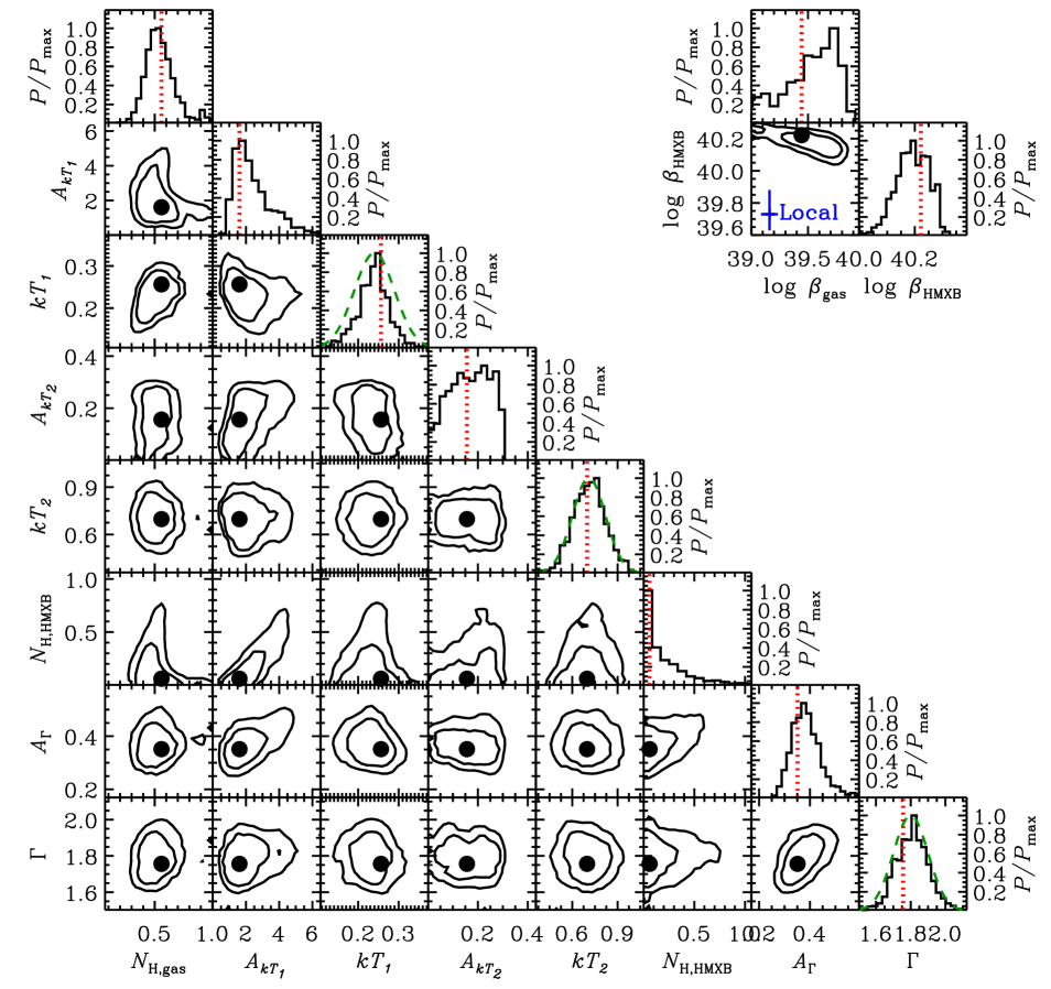
Figure 3: Marginalized 1D and 2D probability distribution functions (PDFs) for the eight parameters in our global model (main corner plot), along with the PDFs for the model-implied scaling relations $\beta_{\_}{\rm HMXB}=L_{\_}{\rm X}$(HMXB)/SFR and $\beta_{\_}{\rm gas}=L_{\_}{\rm X}$(gas)/SFR (upper right). Contours represent 68% and 90% confidence levels. The median model parameter values are shown as vertical dotted lined and filled circles for the 1D and 2D PDFs. The adopted prior distributions on $kT_{\_}1$, $kT_{\_}2$, and $\Gamma$ are shown as dashed curves in their respective 1D PDF diagrams. In the panel showing the 2D PDFs for the scaling relations (i.e., upper right), we show comparison relations for typical local galaxies from Mineo et al. (2012a, hot gas) and Lehmer et al. (2019, HMXBs) (blue cross representing 1$\sigma$ uncertainties). Our model suggests that our sample of low-metallicity star-forming galaxies have both elevated hot gas and HMXB scaling relations over those of typical local galaxies.

5 Results

5.1 The Global Model

As discussed in §4.2, we first fit a photon-energy ($E$) dependent “global” spectral model, $\ell_{\_}E$, which we define as the SFR-normalized intrinsic spectrum in units of luminosity per energy per SFR (e.g., ergs s^-1 keV^-1 yr $M_{\_}\odot^{-1}$). As such, we chose to adopt XSPEC model normalizations that are in intrinsic units. Thus, the $j$th galaxy in our sample will have a model count-rate spectrum, $\phi_{\_}{E,j}$ (uncorrected counts per energy per second per area), and a response-folded model count spectrum, $S_{\_}{E,j}$ (i.e., detected counts per energy channel), calculated following:

$$\phi_{\_}{E,j}={\tt TBABS}_{\_}{\rm Gal,j}*\left(\frac{{\rm SFR}_{\_}j}{4\pi d_{\_}{L,j}^{2}}\frac{\ell_{\_}E}{E}\right)$$ (5)

and

$$S_{\_}{E,j}=\left[{\tt RSP}_{\_}j\left(\phi_{\_}{E,j}\Delta E\right)+{\tt URSP}_{\_}j\left({\rm Bkg}_{\_}{E,j}\right)\right]\times t_{\_}{{\rm exp},j},$$ (6)

where ${\tt TBABS}_{\_}{{\rm Gal},j}$ is the Galactic absorption for the $j$th galaxy (using the $N_{\_}{\rm H,gal}$ values in Col.4 of Table 1), $\Delta E$ represents the energy-dependent channel bin width (in energy units), RSP${}_{\_}j$ and URSP${}_{\_}j$ indicate the use of instrument and flat (unity) responses for the source and background models, respectively, and $t_{\_}{{\rm exp},j}$ is the exposure time for the $j$th galaxy.

The intrinsic model consists of the sum of gas and HMXB contributions, $\ell_{\_}E=\ell_{\_}E({\rm gas})+\ell_{\_}E({\rm HMXB})$, and can be specified in terms of XSPEC models as:

$$\ell_{\_}E({\rm gas})=E{\tt TBABS}_{\_}{\rm gas}*\left({\tt APEC}_{\_}{\rm 1}+{\tt APEC}_{\_}{\rm 2}\right),$$

$$\ell_{\_}E({\rm HMXB})=E\left({\tt TBABS}_{\_}{\rm HMXB}*{\tt POW}_{\_}{\rm HMXB}\right).$$ (7)

Our global fit contains eight free parameters. These include (1) the three normalization terms for the ${\tt APEC}_{\_}{\rm 1}$, ${\tt APEC}_{\_}{\rm 2}$, and ${\tt POW}_{\_}{\rm HMXB}$ components, $A_{\_}{kT_{\_}{\rm 1}}$, $A_{\_}{kT_{\_}{\rm 2}}$, and $A_{\_}\Gamma$, respectively, which have flat priors; (2) the ${\tt TBABS}_{\_}{\rm gas}$ and ${\tt TBABS}_{\_}{\rm HMXB}$ absorption components, $N_{\_}{\rm H,gas}$ and $N_{\_}{\rm H,HMXB}$, respectively, which also have flat priors; (3) the ${\tt APEC}_{\_}{\rm 1}$ and ${\tt APEC}_{\_}{\rm 2}$ temperatures, for which we adopt Gaussian priors with mean and standard deviations $kT_{\_}1=$ $0.24\pm 0.05$ keV and $kT_{\_}2=$ $0.71\pm 0.11$ keV, respectively; and (4) the ${\tt POW}_{\_}{\rm HMXB}$ slope, which has Gaussian priors with mean and standard deviation of $\Gamma=1.8\pm 0.1$.

To fit the data, we started by minimizing $C$ in Eqn. 4 using Sherpa’s optimization algorithm with $kT_{\_}1$, $kT_{\_}2$, and $\Gamma_{\_}{\rm HMXB}$ held fixed at the mean values of their prior distributions. This provides a set of parameters close to the best-fit solution. To sample the full posterior distribution function (PDF) of our model parameters, we utilized a customized adaptive Markov Chain Monte Carlo (MCMC) procedure. In this procedure, we incorporated the additional uncertainties on the limited parameters $kT_{\_}1$, $kT_{\_}2$, and $\Gamma_{\_}{\rm HMXB}$ using their adopted prior distributions (see above). Our MCMC algorithm employs the Metropolis Hastings method (Hastings, 1970), with a vanishing adaptive procedure (see Algorithm 4 from Andrieu & Thoms, 2008). Model parameters are stepped in accordance with a covariance matrix. The covariance matrix is initially set as a diagonal matrix consisting of the Sherpa-derived variances on the five parameters with flat priors that were intially fit (i.e., $N_{\_}{\rm H,gas}$, $A_{\_}{kT_{\_}{\rm 1}}$, $A_{\_}{kT_{\_}{\rm 2}}$, $N_{\_}{\rm H,HMXB}$, and $A_{\_}\Gamma$), plus the prior distribution variances for $kT_{\_}1$, $kT_{\_}2$, and $\Gamma_{\_}{\rm HMXB}$. The covariance matrix is updated at each MCMC step based on the MCMC chain histories, and then used to direct subsequent MCMC steps. The algorithm updates the step sizes in accordance with the covariance matrix until a target optimal acceptance fraction is achieved (Gelman et al., 1996). To satisfy the reversibility criterion for Markov Chains, the adaptive aspect of the algorithm quickly vanishes, and is held fixed for the final 80% of the MCMC trials. The first 20% of the chains are discarded (i.e., “burned”) and the remaining parameter MCMC chains are used to calculate marginalized parameter distributions.

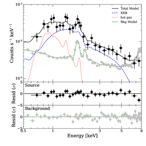
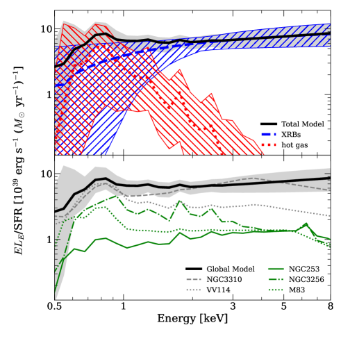
Figure 4: (Left) Stacked average on-source spectrum for the full sample (black circles), $\langle\phi_{\_}E\rangle$ (see Eqn. 5), and rescaled background spectrum (gray circles). For illustrative purposes, the data have been binned by 12 counts and 120 counts for the on-source and background spectra, respectively. Our best-fit global model is shown as a solid black curve, which contains contributions from HMXBs (blue dashed curve), hot gas (red dotted curve), and background (green dashed curve). Residuals to the source and background models are shown in the bottom two panels. (Right) Unfolded global model spectrum, $EL_{\_}E$/SFR, and 16–84% confidence range (black curve with gray envelope). In the top panel, we show model contributions along with their 16–84% confidence ranges (hatched-shaded regions), and in the bottom panel we compare our SED constraint with the NuSTAR comparison galaxies. Our SFR-scaled best-fit spectrum appears elevated over galaxies with nearly solar metallicity (green curves; NGC 253, NGC 3256, and M83) and low-metallicity galaxy VV114 ($\approx$0.3 $Z_{\_}\odot$), but similar to the low-metallicity galaxy NGC 3310 ($\approx$0.2 $Z_{\_}{\odot}$).

Using an MCMC run of 20,000 trials, we sampled the PDF and identified the model that most closely maximizes the posterior as our “best-fit” global model. We note that, given our implementation of non-flat priors, this model is not the same as the model that minimizes the $C$ statistic. To test whether our best-fit global model provides a good fit to the on-source data set for the full sample, we made use of the methods outlined in Bonamente (2019) for calculating the expected value of the $C$ statistic, $C_{\_}{\rm exp}$, and its variance $C_{\_}{\rm var}$, which in the limit of large numbers of bins ($\;\buildrel>\over{\sim}\;$10 bins) and counts ($\;\buildrel>\over{\sim}\;$10 counts) can be taken as a Gaussian distribution that can be used to test the null hypothesis. We computed $C_{\_}{\rm exp}$ and $C_{\_}{\rm var}$ using Eqn. 11 of Bonamente (2019) and computed the null hypothesis probability as

$$p_{\_}{\rm null}=1-{\rm erf}\left(\sqrt{\frac{(C-C_{\_}{\rm exp})^{2}}{2\;C_{\_}{\rm var}}}\right).$$ (8)

Under the above definition, a value of $p_{\_}{\rm null}\approx 1$ indicates $C\approx C_{\_}{\rm exp}$, while deviations of $C$ away from $C_{\_}{\rm exp}$, both low and high, act to reduce the value of $p_{\_}{\rm null}$. For our global model, we calculate $p_{\_}{\rm null}=$ 0.133 (with $C$ being lower than $C_{\_}{\rm exp}$), which indicates that the model is fully compatible with the full data set.

In Figure 3, we show the marginalized 1D and 2D PDFs for the model parameters, and in Table LABEL:tab:glo, we report the values of our best-fit model parameter values, their medians, and 16–84% parameter confidence ranges. In the left panels of Figure 4, we show the stacked best-fit on-source and background spectra for our full sample and the best-fit global and background models and their residuals. In this figure, the background data, and corresponding background model, have been rescaled properly to the source regions, and for illustrative purposes, the data have been binned to 120 background counts per bin and 12 on-source counts per bin; however, note that all fits are performed on unbinned data. The on-source spectrum is best modeled with significant contributions from the three major components, including dominant contributions from hot gas at $\;\buildrel<\over{\sim}\;$1 keV (red dotted curve), HMXBs at $\;\buildrel>\over{\sim}\;$1 keV (blue dashed curve), and background at $\;\buildrel<\over{\sim}\;$0.6 keV and $\;\buildrel>\over{\sim}\;$4 keV (green dashed curve).

Table 3: Global Model Fit Results

Parameter	Units	Best (50% $\pm$ 34%)
$N_{\_}{\rm H,gas}$	$10^{22}$ cm-2	0.56 (0.55${}^{+0.12}_{\_}{-0.10}$)
$A_{\_}{kT_{\_}1}^{\dagger}$		1.61 (3.00${}^{+1.85}_{\_}{-1.20}$)
$kT_{\_}1$	(keV)	0.26 (0.24${}^{+0.03}_{\_}{-0.04}$)
$A_{\_}{kT_{\_}2}^{\dagger}$		0.16 (0.21${}^{+0.06}_{\_}{-0.09}$)
$kT_{\_}2$	(keV)	0.70 (0.73${}^{+0.11}_{\_}{-0.11}$)
$N_{\_}{{\rm H,HMXB}}$	$10^{22}$ cm-2	0.06 (0.50${}^{+0.51}_{\_}{-0.31}$)
$A_{\_}\Gamma^{\ddagger}$		0.35 (0.39${}^{+0.07}_{\_}{-0.05}$)
$\Gamma$		1.76 (1.82${}^{+0.09}_{\_}{-0.10}$)
Scaling Relations⋆
$\log L_{\_}{\rm 0.5-8~{}keV}$/SFR	ergs s-1 ($M_{\odot}$ yr-1)-1	40.29 (40.29${}^{+0.03}_{\_}{-0.03}$)
$\log L_{\_}{\rm 0.5-2~{}keV}^{\rm gas}$/SFR	ergs s-1 ($M_{\odot}$ yr-1)-1	39.44 (39.58${}^{+0.17}_{\_}{-0.28}$)
$\log L_{\_}{\rm 0.5-8~{}keV}^{\rm HMXB}$/SFR	ergs s-1 ($M_{\odot}$ yr-1)-1	40.22 (40.19${}^{+0.06}_{\_}{-0.06}$)
$\log L_{\_}{\rm 0.2-2~{}keV}$/SFR	ergs s-1 ($M_{\odot}$ yr-1)-1	39.96 (39.94${}^{+0.04}_{\_}{-0.03}$)
Goodness of Fit Evaluation
$C$		2426
$C_{\_}{\rm exp}$		2576
$C_{\_}{\rm var}$		9908
$p_{\_}{\rm null}$		0.133

^†The values of the hot gas normalization represent the quantity $4\pi d_{\_}L^{2}$/SFR $10^{-14}/(4\pi d_{\_}A^{2}[1+z]^{2})\int_{\_}Vn_{\_}{\rm H}n_{\_}edV$ cm^-5 ($M_{\_}\odot$ yr^-1)^-1 Mpc², where $d_{\_}L$ is the luminosity distance in Mpc, SFR is in units of $M_{\_}\odot$ yr^-1, $d_{\_}A$ is the angular diameter distance in cm, $z$ is the redshift, $n_{\_}{\rm H}$ and $n_{\_}e$ are hydrogen and electron densities in units of cm^-3. See https://heasarc.gsfc.nasa.gov/xanadu/xspec/manual/XSmodelApec.html for a full description of the APEC model.
^‡ The power law model normalization has units of photons keV^-1 cm^-2 s^-1 ($M_{\_}\odot$ yr^-1)^-1 Mpc² at 1 keV.
^⋆Uncertainties on scaling relations are based on MCMC chains of the scaling relations themselves and represent 16–84% 1D uncertainties marginalized over all parameters.

In the top-right panel of Figure 4, we show the unfolded global model spectrum, in terms $EL_{\_}E$/SFR (where $L_{\_}E\equiv\ell_{\_}E$ SFR and $EL_{\_}E=\nu L_{\_}\nu$) and its HMXB and hot gas model contributions. The gray shaded region shows the full range of spectral models for the 68% of models with the highest posterior probabilities. The bottom-right panel of Figure 4 displays the same spectrum, but with comparisons to the galaxies presented in Lehmer et al. (2015) and Garofali et al. (2020) (see red stars in Fig. 2 for property comparison). For ease of comparison, we used gray coloring for NGC 3310 (dashed) and VV114 (dotted), which have low metallicities of $Z\approx 0.2Z_{\_}\odot$ and $0.3Z_{\_}\odot$, respectively, that are comparable to the galaxies in our sample. The remaining galaxies (i.e., NGC 253, NGC 3256, and M83, shown as green curves in Fig. 4) are nearly solar metallicity.

We find that the SFR-normalized X-ray spectrum for our low-metallicity galaxy sample is elevated compared to solar-metallicity galaxies, somewhat elevated compared to VV114, and similar to the low-metallicity galaxy NGC 3310. The elevation of our sample X-ray spectrum over that found in solar-metallicity galaxies appears to apply to both XRB and hot gas components; however, the effect is of larger magnitude for the HMXB component. Integration of our global model provides a prediction for the luminosity scaling relation with SFR. Given the construction of our model, this integration can be performed for both the full spectrum and portions of the spectrum of interest, such as the HMXB and hot gas components. To calculate confidence intervals, we computed such integrations at each step of our MCMC procedure and thus sampled their marginalized PDFs. Throughout the remainder of this paper, we choose to assess HMXB scaling relations with SFR using the 0.5–8 keV band and hot-gas scaling relations with SFR using the 0.5–2 keV band; hereafter we define these relations as $\beta_{\_}{\rm HMXB}=L_{\_}{\rm 0.5-8~{}keV}^{\rm HMXB}$/SFR and $\beta_{\_}{\rm gas}=L_{\_}{\rm 0.5-2~{}keV}^{\rm gas}$/SFR, where $\beta$ is quoted in units of erg s^-1 ($M_{\odot}$ yr^-1)^-1. These choices were adopted due to both components providing significant contributions to the overall spectra in the chosen bands and the availability of published scaling relations that use the same bandpasses (e.g., Mineo et al., 2012a; Lehmer et al., 2019, 2021).

In the upper-right panels of Fig. 3 we display the 1D and 2D marginalized PDFs for $\beta_{\_}{\rm HMXB}$ and $\beta_{\_}{\rm gas}$ and show comparison values from the local studies of Lehmer et al. (2019) and Mineo et al. (2012a), respectively. The median values and 16–84% confidence intervals for $\beta_{\_}{\rm HMXB}$ and $\beta_{\_}{\rm gas}$ are

$$\log L_{\_}{\rm 0.5-8~{}keV}^{\rm HMXB}{\rm/SFR}=\log\beta_{\_}{\rm HMXB}=40.19\pm 0.06,$$ (9)

$$\log L_{\_}{\rm 0.5-2~{}keV}^{\rm gas}{\rm/SFR}=\log\beta_{\_}{\rm gas}=39.58^{+0.17}_{\_}{-0.28},$$ (10)

which are listed in Table LABEL:tab:glo along with the maximum posterior values. Here, we note that our derived values of $\beta_{\_}{\rm HMXB}$ and $\beta_{\_}{\rm gas}$ for our sample are both significantly elevated compared to local scaling relations. In § 6 below, we discuss in more detail possible explanations for the elevation of these relations.

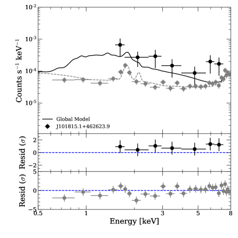
Figure 5: Chandra spectrum of J101815.1+462623.9 (filled black circle with 1$\sigma$ uncertainties), the only galaxy in our sample that is poorly fit by both our rescaled and global models (black curve). The residuals to the global model (middle panel) suggest that this source has a somewhat flatter X-ray spectrum than the sample average, and contains notable excesses near the Fe K region at 6–7 keV. As such, this object plausibly contains a heavily-obscured/Compton-thick AGN.

5.2 Individual Source Models

To investigate galaxy-to-galaxy variations in the spectra of the galaxies in our sample, we fit each galaxy spectrum individually using a “scaled model,” which consists of our global model (§ 5.1) rescaled by a multiplicative constant factor (CONSTANT in xspec). Here, all parameters of the global model were held fixed at the global best-fit values displayed in Table LABEL:tab:glo, and we fit each galaxy using a single multiplicative scaling parameter $A_{\_}{\rm cnst}$.

For each galaxy, we identified best-fit values and PDFs of $A_{\_}{\rm cnst}$ using $C$ in Eqn 3 (here we adopt minimum $C$ values as our best-fit models), and we calculated null-hypothesis probabilities using Eqn 8. In Col.(6) of Table 2, we report the best-fit values of $A_{\_}{\rm cnst}$, the statistical results of the fit, and calculated 0.5–8 keV fluxes and luminosities for the single-parameter model (see Col.7–12). We also provide, in Col.(13)–(16), the results for the case of the global model (i.e., $A_{\_}{\rm cnst}=1$) for comparison.

From random statistical scatter, we expect $\approx$1–2 objects will have $p_{\_}{\rm null}^{\rm src}\lower 2.15277pt\hbox{$\;\buildrel<\over{\sim}\;$}0.05$, which we adopt as a threshold for statistical acceptability. We find that all scaled-model fits are statistically acceptable, with $p_{\_}{\rm null}^{\rm src}>0.05$, suggesting that our modeling does not require variations in spectral shape to describe the data. We note, however, that our galaxies have small numbers of net counts and poor constraints on individual bases.

For the global model itself, which has no free parameters for an individual galaxy, we find that most galaxies are in good agreement with the direct model predictions, with the exception of four sources that show some tension with the model ($p_{\_}{\rm null}^{\rm gl}\leq 0.05$). Among these four sources, the poorest fitting sources are J165844.5+351923.0 and J101815.1+462623.9. The former object appears to have a deficit of observed counts, compared to those expected from the relation. We expect that this could plausibly arise due to stochastic sampling of the HMXB XLF, which has been shown to produce an additional source of galaxy-to-galaxy scatter that skews the distribution of $L_{\_}{\rm 0.5-8~{}keV}^{\rm HMXB}$ to low values (see, e.g., Gilfanov et al., 2004; Justham & Schawinski, 2012; Lehmer et al., 2019).

The latter galaxy that is poorly fit by our global model, J101815.1+462623.9, is also the most poorly fit by our scaled model, suggesting some deviation of the spectral shape of this source with respect to the global-model shape. In Fig 5, we show the spectrum of J101815.1+462623.9 and the global model prediction of its spectrum. Visual inspection of the spectrum and its residuals to the global model suggest that this source has a somewhat flatter spectral shape (i.e., lower values of $\Gamma$) with elevated residuals between 6–7 keV, where the Fe K line complex is found. These spectral features (flat spectral slope and potential Fe K feature), along with the fact that our objects were selected to have optical spectral features consistent with normal star-forming galaxies, suggests that this object is a good candidate for harboring a heavily-obscured or Compton-thick AGN. However, given that this source has been detected with only $\approx$20 net counts, we do not attempt to derive any detailed parameters using more complex models.

6 Discussion

6.1 The HMXB X-ray/SFR Scaling Relation and Scatter

In Figure 6, we display the HMXB model component luminosity, $L_{\_}{\rm 0.5-8~{}keV}^{\rm HMXB}$, versus SFR for our sample. The HMXB luminosities were computed using the scaled model fits to each galaxy. We have overlaid our global scaling relation, $\log\beta_{\_}{\rm HMXB}=40.19\pm 0.06$. Given that the global model provides a reasonable description of the majority of the galaxy X-ray spectra without adjustment, it is not surprising that the global model agrees well with the majority of the $L_{\_}{\rm 0.5-8~{}keV}^{\rm HMXB}$ values.

The metallicity-dependent HMXB XLF work by L21 provides direct constraints on the $L_{\_}{\rm 0.5-8~{}keV}^{\rm HMXB}$-SFR relation as a function of metallicity through the integration of their HMXB XLF models. By construction, our sample contains a narrow distribution of metallicities, with mean and 1$\sigma$ standard deviation of $12+\log({\rm O}/{\rm H})$ = $8.16\pm 0.03$ ($Z=[0.29\pm 0.02$] $Z_{\_}\odot$). At the sample mean, L21 predict $\log\beta_{\_}{\rm HMXB}^{\rm L21}(Z=0.3Z_{\_}\odot)=39.97\pm 0.12$, which we display in Figure 6 as a dashed orange line with hatched uncertainty region. This value is somewhat lower than the value found for our sample, albeit within the current uncertainties.

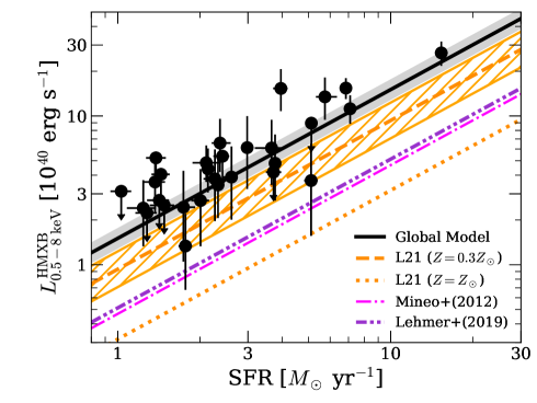
Figure 6: HMXB component 0.5–8 keV luminosity, $L_{\_}{\rm 0.5-8~{}keV}^{\rm HMXB}$ versus SFR for the 30 galaxies in our sample (filled circles with 1$\sigma$ error bars or 90% confidence upper limits). $L_{\_}{\rm 0.5-8~{}keV}^{\rm HMXB}$ was calculated for each galaxy using the scaled model described in § 5.2. Our global best-fit model scaling relation, $\beta_{\_}{\rm HMXB}$, is displayed as a solid black line with a grey shaded region representing the 1$\sigma$ uncertainty. For comparison, we show the local HMXB relations from Mineo et al. (2012b, magenta dot-dashed line) and Lehmer et al. (2019, purple dot-dot-dashed line), as well as the metallicity-dependent scaling relation from L21 for solar metallicity (dotted orange line) and 0.3 $Z_{\_}\odot$ (dashed orange line with 1$\sigma$ hatched region), the latter of which is representative of the metallicity of our sample.

For comparison, we also display Figure 6, the solar-metallicity model from L21, which lies at $\log\beta_{\_}{\rm HMXB}^{\rm L21}(Z=Z_{\_}\odot)=39.50\pm 0.11$, a factor of $\approx$4 times lower than our sample. We also show “local” estimates of $\log\beta_{\_}{\rm HMXB}$ from the work of Mineo et al. (2012b) and Lehmer et al. (2019), which are based on samples of nearby star-forming galaxies that span a non-negligible range of metallicity. After correcting for differences in the Mineo et al. (2012b) IMF, these samples have values of $\log\beta_{\_}{\rm HMXB}=39.67\pm 0.06$ and $\log\beta_{\_}{\rm HMXB}=39.71^{+0.14}_{\_}{-0.09}$ for Mineo et al. (2012b) and Lehmer et al. (2019), respectively. These values lie between those of our sample and the L21 solar-metallicity prediction. For the Lehmer et al. (2019) sample, which quotes metallicity values, galaxies with sSFR $\lower 2.15277pt\hbox{$\;\buildrel>\over{\sim}\;$}10^{-10}$ yr^-1, which are dominated by HMXB populations, have metallicities of $\approx$0.8 $Z_{\_}\odot$. At this metallicity, L21 predict $\log\beta_{\_}{\rm HMXB}^{\rm L21}(Z=0.8Z_{\_}\odot)=39.64\pm 0.11$, consistent with the Lehmer et al. (2019) value for local galaxies.

The above comparisons of point-source studies of HMXBs with the constraints from our galaxies, suggests near consistency when the $L_{\_}{\rm X}$(HMXB)/SFR scaling relation is put into context with galaxy metallicity. To further test this connection, we investigated the scatter of the X-ray emission from our galaxy population, as measured by the distribution of 0.5–8 keV counts. As discussed in § 5.1 of L21, incomplete sampling of the HMXB XLF can lead to non-negligible scatter of $L_{\_}{\rm X}$(HMXB) for a given SFR. The magnitude of this scatter is predicted to increase with decreasing SFR. For the L21 HMXB XLF model at $\approx$0.3 $Z_{\_}\odot$, the scatter is expected to decline from $\approx$0.5 dex to 0.1 dex over SFR = 1–10 $M_{\odot}$ yr^-1, a range covered by our galaxy sample.

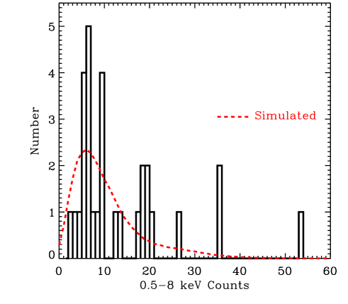
Figure 7: Observed distribution of on-source 0.5–8 keV counts (black histogram; see Col.(4) in Table 2). The dashed red curve shows the expected distribution from simulations that include HMXB emission and stochastic fluctuations from sampling of the L21 HMXB model XLF, plus minor contributions from hot gas, local background levels, and Poisson fluctuations. A K-S test indicates that the observed and expected distributions are consistent, suggesting the scatter in our galaxy sample is also consistent with expected scatter from HMXB populations.

To test more explicitly whether our sample data are consistent with HMXB XLF model framework from L21, we simulated the expected distributions of on-source counts for each of our galaxies and compared those distributions to our observations. For a given galaxy, we first used the SFR and $12+\log({\rm O}/{\rm H})$ values as input to the L21 HMXB XLF model, which specifies the expected HMXB XLF shape and normalization for the galaxy. Next, treating the HMXB XLF model as a probability distribution function, we drew HMXB luminosities from that distribution to generate simulated HMXB populations that could plausibly be expected from within the galaxy. Summing the luminosity contributions from a given simulated HMXB population provides an estimate of the integrated HMXB population luminosity. We performed 5000 simulations for each galaxy to form a distribution of expected HMXB luminosities expected from the population. We then converted the simulated HMXB luminosities into contributions to the source counts, using the $L_{\_}{\rm 0.5-8~{}keV}^{\rm HMXB}$–to–counts conversion factor appropriate for the galaxy. We then added the background count estimate from Col.(5) in Table 2 and the expected hot gas model contribution to the total counts based on our best-fit model. We note that while some variation in the intrinsic hot gas emission is expected, this variation has not been well characterized observationally or theoretically and is not included in our simulations. However, our best-fit model predicts that HMXBs provide a factor of $\approx$2–4 (median 3.8) times more counts than the hot gas component, suggesting that unmodeled variations in hot gas emission are likely to have a negligible impact on our results.

For a given simulation, the combined HMXB, hot gas, and background counts estimates for a given galaxy are summed and subsequently perturbed using a Poisson distribution with a mean equal to the summed counts. This results in 5,000 distributions of simulated on-source counts for the sample. Combining all of the simulations together provides a smooth distribution of model-expected on-source counts for our sample, which we display in Figure 7, along with the actual observed counts distribution. A two-sided K-S test between the simulated counts and our data suggest that the two distributions are statistically consistent with each other ($p_{\_}{KS}=0.18$). Thus, the observed distribution of counts from our sources is consistent with the combination of noise from our data and expected HMXB XLF scatter.

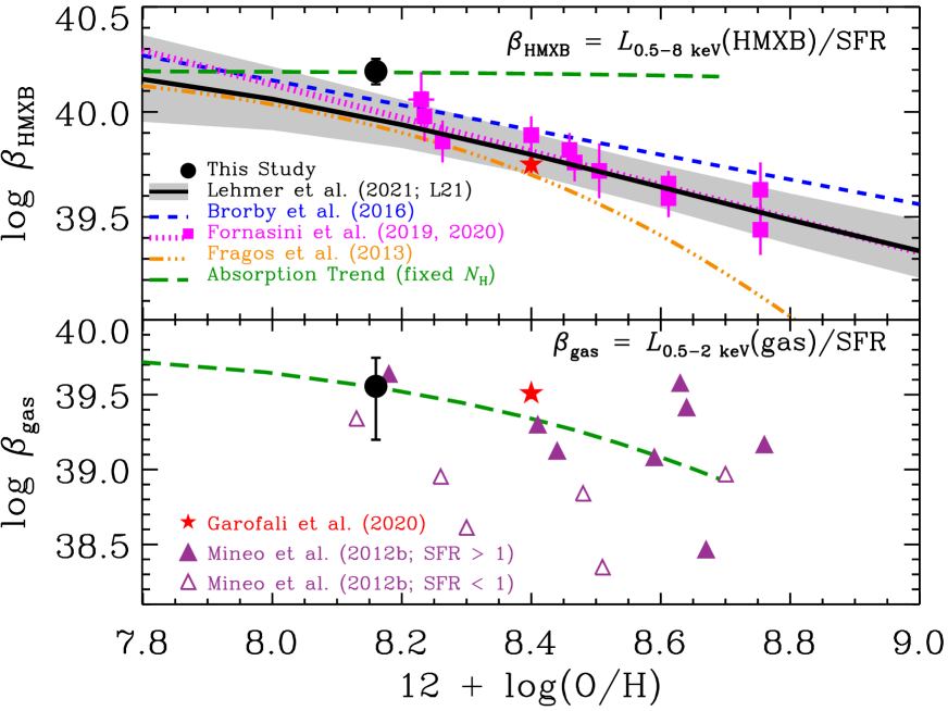
Figure 8: ($a$) Logarithm of the 0.5–8 keV HMXB luminosity per SFR, $\beta_{\_}{\rm HMXB}$ versus galaxy metallicity for our galaxy sample (black filled circle with 1$\sigma$ uncertainties) and 12 stacked subsamples of $z\approx$ 0.1–2.6 galaxies from Fornasini et al. (2019, 2020, magenta filled squares with 1$\sigma$ uncertainties). The L21 relation and its 16–84% confidence interval are shown as a solid curve and gray shaded region, respectively. For comparison, the empirical relations from Fornasini et al. (2020, dotted magenta curve) and Brorby et al. (2016, short-dashed blue curve), as well as the XRB population synthesis model prediction from Fragos et al. (2013b, triple-dot-dashed orange curve) are overlaid. Our new constraint on $\beta_{\_}{\rm HMXB}$ is somewhat elevated compared to that expected from $L_{\_}{\rm X}$-SFR-$Z$ relations in the literature, potentially due to our galaxies containing relatively young and unobscured HMXB populations. The green long-dashed curve highlights the expected effect of varying metallicity for a fixed column density of $N_{\_}{\rm H}=6\times 10^{21}$ cm^-2, and illustrates that the data are not consistent with being driven solely by the effects of metallicity on absorption. ($b$) Logarithm of the 0.5–2 keV hot gas luminosity per SFR, $\beta_{\_}{\rm gas}$, versus metallicity ($12+\log({\rm O}/{\rm H})$) for our sample and the point-source-excised analyses of 16 galaxies with metallicity estimates in Mineo et al. (2012a, purple triangles) and VV114 (Garofali et al., 2020, filled red star). The Mineo et al. (2012a) sample spans a broader range of SFR than our sample, and we use filled triangles to represent galaxies with SFR $>1$ $M_{\odot}$ yr^-1, consistent with the range of our sample, and open triangles represent galaxies with SFR $<1$ $M_{\odot}$ yr^-1. The effects of metallicity on absorption (green long-dashed curve) are expected to be significant for $\beta_{\_}{\rm gas}$ and may play a role in the observed trend.

6.2 Metallicity Dependence of HMXB and Hot Gas Scaling Relations

In § 5.1, we showed that our global fit yields constraints on the scaling relations $\beta_{\_}{\rm HMXB}$ and $\beta_{\_}{\rm gas}$ that are elevated compared to scaling relations derived for more representative local galaxies (e.g., Mineo et al., 2012b, a; Lehmer et al., 2019, see marginalized distributions in Fig. 3). As shown in §6.1, the elevation of $\beta_{\_}{\rm HMXB}$ can be attributed primarly to the metallicity-dependence of the $L_{\_}{\rm X}$(HMXB)-SFR-$Z$ relation, as has been presented in the literature (see §1); however, there is some evidence that our relation is further enhanced over such relations.

To provide context to our results in terms of potential metallicity dependencies, we constructed Figure 8, which displays $\beta_{\_}{\rm HMXB}$ (Fig. 8$a$) and $\beta_{\_}{\rm gas}$ (Fig. 8$b$) as a function of metallicity. The black curve in Figure 8$a$ shows the L21 relation and its 1$\sigma$ uncertainty. For comparison, we also show the XRB population synthesis prediction from Fragos et al. (2013b, orange triple-dot-dashed curve), the $L_{\_}{\rm X}$(HMXB)-SFR-$Z$ relations from Brorby et al. (2016, blue short-dashed line) and Fornasini et al. (2020, magenta dotted line), and the stacked constraints from Fornasini et al. (2019, 2020, magenta filled squares with 1$\sigma$ error bars), the latter of which are based on $z\approx$ 0.1–2.6 galaxy samples that include 20–400 galaxies per data point. In this context, our estimate of $\beta_{\_}{\rm HMXB}$ (black filled circle with 1$\sigma$ error bars) is elevated by a factor of 1.2–1.5 times that expected from L21, Fornasini et al. (2020), and Brorby et al. (2016) relations.

We speculate that an elevated value of $\beta_{\_}{\rm HMXB}$ for our sample, compared with $L_{\_}{\rm X}$(HMXB)-SFR-$Z$ relations may be expected due to our sample having (1) somewhat lower HMXB intrinsic absorption than other samples (e.g., $N_{\_}{\rm H,HMXB}\lower 2.15277pt\hbox{$\;\buildrel<\over{\sim}\;$}10^{21}$ cm^-2 for our sample versus $\approx 6\times 10^{21}$ cm^-2 from L21; see $\S$ 5.1); and (2) relatively high sSFRs, and thus, younger stellar populations compared to the galaxies used to derive local relations (see Fig. 2 for comparison with other samples). Regarding the latter point, a recent study of galaxies in the Chandra Deep Field-South by Gilbertson et al. (2021) found that $L_{\_}{\rm X}/M_{\_}\star$ for HMXBs declines by nearly an order of magnitude from 10 Myr to 100 Myr. As such, galaxies with relatively young stellar populations, like our sample, may have elevated $\beta_{\_}{\rm HMXB}$ compared to more representative galaxy samples. Additional evidence for enhanced X-ray emission (relative to relations) has been noted for galaxy samples that are selected explicitly to have signatures of very young stellar populations (e.g., from Lyman-continuum emitters and green peas; Bluem et al., 2019; Svoboda et al., 2019; Franeck et al., 2022). For example, Svoboda et al. (2019) find that the two X-ray-detected green peas in their sample have soft spectra with X-ray luminosities on the order of $10^{42}$ erg s^-1. Given their SFR $\approx$ 20–40 $M_{\odot}$ yr^-1 (after correcting to our adopted IMF; see green downward triangles in Fig. 2), these $L_{\_}{\rm X}$/SFR values are $\approx$2–3 times higher than observed for the galaxies in our sample. Considering the stellar masses of these galaxies of $\approx$few $\times 10^{9}$ $M_{\odot}$, this implies $L_{\_}{\rm X}/M_{\_}\star\approx 10^{31}$ ergs s^-1 $M_{\_}\odot^{-1}$, a value consistent with stellar populations of $\;\buildrel<\over{\sim}\;$100 Myr in age (see Gilbertson et al., 2021, for details).

Fewer constraints on the metallicity dependence of $\beta_{\_}{\rm gas}$ are available in the literature, and no formal relations have been proposed. In Figure 8$b$, we show our estimate of $\beta_{\_}{\rm gas}$ along with estimates for 14 individual galaxies from Mineo et al. (2012a, purple triangles) that have metallicities extracted from the literature (see Basu-Zych et al. 2013a for details) and VV114 from Garofali et al. (2020, red star). The Mineo et al. (2012a) and Garofali et al. (2020) constraints on $\beta_{\_}{\rm gas}$ are based on careful measurements of the diffuse emission after excising X-ray point source contributions and are expected to be highly reliable. A Spearman’s rank test suggests that there is no significant correlation between $\beta_{\_}{\rm gas}$ and $12+\log({\rm O}/{\rm H})$, when including our constraint and those in the literature ($\rho=-0.32$ for 16 data points). However, if we restrict the comparison sample to include only galaxies with SFR $\;\buildrel>\over{\sim}\;$ 1 $M_{\odot}$ yr^-1 that are comparable to our sample and less subject to statistical scatter than lower-SFR galaxies, we find a 95% significant ($\rho=-0.63$ for 10 data points) anticorrelation.

If $\beta_{\_}{\rm gas}$ is indeed anticorrelated with metallicity, there are potential physical reasons that could explain such a trend. As highlighted in §4.2, hot gas emission has been studied extensively in nearby galaxies (see discussion and citations in §4.2). While we expect that our simple thermal model – a two-temperature plasma with absorption by an ISM with solar abundance – will be sufficient to extract a reliable measurement of $\beta_{\_}{\rm gas}$, we do not assume that our model provides a faithful description of the full physical picture. Detailed studies of resolved nearby galaxies find that distributions of plasma temperatures are inevitably present (e.g., Strickland & Stevens, 2000; Strickland et al., 2004; Kuntz & Snowden, 2010; Lopez et al., 2020; Wang et al., 2021) and the efficiency of converting mechanical heating of the ISM into hot gas X-ray emission depends on star-formation timescales that are shorter than those measured for typical galaxies (e.g., McQuinn et al., 2018; Gilbertson et al., 2021). Therefore, it seems plausible that variations in star-formation history and physical environment (e.g., galaxy morphology and gravitational potential) will lead to variations in $\beta_{\_}{\rm gas}$. For local galaxies, these factors are often correlated with metallicity. We can also expect that both the absorbing and emitting ISM will be influenced by metallicity. For a fixed hydrogen column density and fixed intrinsic $L_{\_}{\rm X}^{\rm gas}$/SFR ratio, the escaping low-energy emission (i.e., $\beta_{\_}{\rm gas}$) will decline with increasing metallicity due to the increasing impact of metal absorption lines (particularly from C, O, Ne, and Fe L).

While the low signal-to-noise X-ray spectra in this study and in the literature are insufficient to reliably constrain directly the metallicities of the absorbing ISMs, we can determine theoretically the effect of varying ISM abundance on emergent X-ray emission. In Figure 8, we show how $\beta_{\_}{\rm HMXB}$ and $\beta_{\_}{\rm gas}$ would be impacted by metallicity variations for fixed values of $N_{\_}{\rm H}$ and intrinsic $L_{\_}{\rm X}$/SFR (green dashed curves). The displayed curves are anchored to the best-fit values of $\beta_{\_}{\rm HMXB}$ and $\beta_{\_}{\rm gas}$ and mean $12+\log({\rm O}/{\rm H})$ from this study and assume the best-fit $N_{\_}{\rm H}$ values (see Table LABEL:tab:glo). Since absorption primarily affects the emergent low-energy emission, $\beta_{\_}{\rm HMXB}$ (calculated for the 0.5–8 keV band) is not strongly impacted by metallicity-dependent absorption, and the observed $L_{\_}{\rm X}$(HMXB)-SFR-$Z$ relation is inconsistent with being driven by absorption (at least in the 0.5–8 keV band). However, the predicted impact on $\beta_{\_}{\rm gas}$ (derived in the 0.5–2 keV band) is significant across $Z\approx$ 0.2–1 $Z_{\_}\odot$, and the metallicity-dependent trajectory appears to be consistent with the published constraints for SFR $\;\buildrel>\over{\sim}\;$ 1 $M_{\odot}$ yr^-1 galaxies (by visual inspection).

While a detailed investigation of the dependencies of $\beta_{\_}{\rm gas}$ on physical properties is beyond the scope of the current paper, this tantalizing result calls for future studies on how hot gas emission varies with galaxy properties like metallicity and star-formation history. As we outline in the next section, since hot gas emission dominates at low X-ray energies in star-forming galaxies, it may also provide important contributions to ISM ionization and IGM heating in low-metallicity galaxies.

6.3 The X-ray–to–IR Emergent and Intrinsic SED

As discussed in §1, sources of high-energy emission, like hot gas and HMXBs, could provide substantial long-range heating of the IGM in the early Universe and ionizing radiation to galaxy ISMs. However, the potential for these sources to have significant impacts depends on how these models are extrapolated into the EUV and soft X-ray bands (0.01–0.5 keV), where no direct observational constraints are available. Here we provide model constraints on the SFR-normalized SED of our sample across a broad wavelength range, spanning the near-IR ($\approx$1$\mu$m) to hard X-rays ($\approx$30 keV). Our models include contributions from stellar, nebular, and dust models from Lightning, as discussed in §3, and global-model constraints to the hot gas and HMXB emission (see §§4.2 and 5.1).

Table 4: SFR-Normalized Model SED

		$EL_{\_}E$/SFR ($10^{40}$ erg s-1 ($M_{\odot}$ yr-1)-1)
		Emergent SED				Intrinsic SED
$\log\lambda($Å$)$	$\log E({\rm keV})$	stellar	hot gas	HMXBs	Total	stellar	hot gas	HMXBs	Total
(1)	(2)	(3)	(4)	(5)	(6)	(7)	(8)	(9)	(10)
4.07	$-$2.98	441	0.0150	0.0552	442	445	0.0150	0.0552	446
4.02	$-$2.93	493	0.0084	0.0569	494	500	0.0084	0.0569	501
3.98	$-$2.88	531	0.0000	0.0587	532	542	0.0000	0.0587	543
3.93	$-$2.84	554	0.0110	0.0605	555	569	0.0110	0.0605	569
3.89	$-$2.79	592	0.0462	0.0624	592	611	0.0462	0.0624	612
3.84	$-$2.75	650	0.0232	0.0644	650	668	0.0232	0.0644	669
3.79	$-$2.70	698	0.0173	0.0665	698	733	0.0173	0.0665	733
3.75	$-$2.65	752	0.0866	0.0687	753	800	0.0866	0.0687	800
3.70	$-$2.61	848	0.0184	0.0709	849	882	0.0184	0.0709	883
3.66	$-$2.56	878	0.0305	0.0737	879	959	0.0305	0.0737	960

Note. — This table is available in its entirety in machine-readable form. Only an abbreviated version of the table is shown here to illustrate form and content.

For the purpose of obtaining interpolations of our models into the EUV and soft X-ray range that are as realistic as possible, we modified the stellar and HMXB components used to model our data in the following ways. For the stellar model, we utilized our Lightning-based SED for wavelengths shorter than the Lyman break at 912 Å, and extrapolated the models into the EUV using BPASS v. 2.2.1 (Eldridge et al., 2017; Stanway & Eldridge, 2018) SEDs. This choice is motivated by the fact that the BPASS models both extend further into the EUV than those of Lightning and include modeling of stellar atmospheres in interacting binary stars, which can provide important contributions to the EUV. For this extrapolation, we adopted the binary-star BPASS models corresponding to a metallicity of $Z\approx 0.3Z_{\_}\odot$ and a Chabrier (2003) IMF with an upper-mass cutoff at 300 $M_{\_}\odot$. When adopting the SFH obtained by Lightning, we found that the BPASS SED was similar to our Lightning-based SED at wavelengths longer than the Lyman break, where the SEDs are constrained by our data.

We modified the HMXB model component from a simple power-law model to a more physically motivated ULX model that is consistent with our X-ray data. To identify a suitable physically motivated HMXB component, we inspected the ULX spectra studied by Walton et al. (2018) and found that the spectral model for Ho IX X-1 was the most similar in 0.5–8 keV shape to that of our X-ray spectral model and chose to adopt the Ho IX X-1 model fits for our extrapolations. Walton et al. (2018) model Ho IX X-1 using the combination of a standard radiatively-efficient accretion disk (DISKBB) for the outer portions of the accretion disk, a geometrically thick disk with modified temperature gradient (DISKPBB) for the inner portion of the accretion disk, and a cut-off power-law to account for Comptonization from either an accretion column (for a NS accretor) or a funnel-like beaming medium (BH case Walton et al., 2017). We thus constructed our modified HMXB SED component using the Ho IX X-1 model from Walton et al. (2018), but with our best-fit value of the absorption column density and normalization adjusted to fit our data. We found that this approach produced a nearly equivalent quality fit to the observed data as that reported in §5.1.

In Figure 9, we show the resulting model over the energy range $E=$ 0.001–30 keV ($\lambda=$ 0.4–12,400Å) both as the emergent SED (Fig. 9$a$) and intrinsic SED (Figs. 9$b$ and 9$c$) models. The emergent SED model includes stellar, nebular, and dust emission, attenuation from the nebula and dust, as well as attenuated hot gas and HMXB emission. The intrinsic SED model includes unattenuated stellar, hot gas, and HMXB emission, and does not include attenuation and emission from nebulae and dust. In Table 4, we tabulate the numerical values of our model spanning the broader wavelength range of 1$\mu$m to 30 keV. We also provide model-based uncertainties for our emergent SED following the procedures discussed in $\S$5.1, and the gray shaded region in Figure 9$a$ represents 16–84% confidence intervals for both the combined Lightning SED models and our global model fits to the Chandra data. Despite our efforts to provide uncertainties, we emphasize that these uncertainties are underestimated in the EUV range (0.01–0.5 keV), as they only include uncertainties on extrapolated model components constrained outside of this range. Additional emission in the EUV range may arise from varied model extrapolations or additional hot thermal components that do not contribute significantly outside the EUV.

6.3.1 The Emergent SED

The emergent SED of our sample (Fig. 9$a$) provides a benchmark for comparing with 21 cm studies of the impact of X-ray heating on the high-redshift IGM (see §1 for discussion). A recent first result from the HERA collaboration (The HERA Collaboration et al., 2021) provided new upper limits on the 21 cm power-spectrum fluctuations from the IGM at $z\approx$ 8 and 10. Using the HERA limits, along with galaxy and IGM property constraints (e.g., galaxy UV luminosity function and Ly$\alpha$ forest constraints on the IGM opacity), they placed constraints on the spin temperature and the average galaxy $L_{\_}{\rm<2~{}keV}^{\rm ion}$/SFR ratio required to heat the IGM to those levels. The quantity $L_{\_}{\rm<2~{}keV}^{\rm ion}$/SFR is defined as the ionizing X-ray radiation between 0.2–2 keV that escapes to the IGM.

As discussed in §2, our galaxy sample was selected to have properties that were comparable to star-forming active galaxies that may have provided a substantial fraction of the X-ray radiation field at $z\sim$ 6–10. Although a detailed estimate of the average $L_{\_}{\rm<2~{}keV}^{\rm ion}$/SFR ratio for galaxies at $z\sim 10$ would require detailed knowledge of the distribution of metallicities and X-ray spectral models for galaxies with a variety of properties, it is instructive to compare our sample constraints with those from HERA. For our models, we calculate the quantity $L_{\_}{\rm 0.2-2~{}keV}$/SFR (equivalent to $L_{\_}{\rm<2~{}keV}^{\rm ion}$/SFR) and propagate its uncertainties following the methods discussed in §5.1. The HERA collaboration find $\log L_{\_}{\rm<2~{}keV}^{\rm ion}$/SFR = 40.2–41.9 (68% confidence highest posterior density), as compared with our value of $\log L_{\_}{\rm 0.2-2~{}keV}$/SFR = $39.94^{+0.04}_{\_}{-0.03}$ for our model. We note that the HERA 1D PDF has a broad tail toward low values of $\log L_{\_}{\rm<2~{}keV}^{\rm ion}$/SFR, and our value of $\log L_{\_}{\rm 0.2-2~{}keV}$/SFR is well within the 95% confidence range, which extends to just below $\log L_{\_}{\rm 0.2-2~{}keV}$/SFR $\approx 39$. Thus, our constraints are currently compatible with those of HERA. Future, improved constraints from HERA are expected to help put into context the X-ray spectral constraints established here and the X-ray radiation field generated from galaxies in the early Universe (at $z\approx 10$).

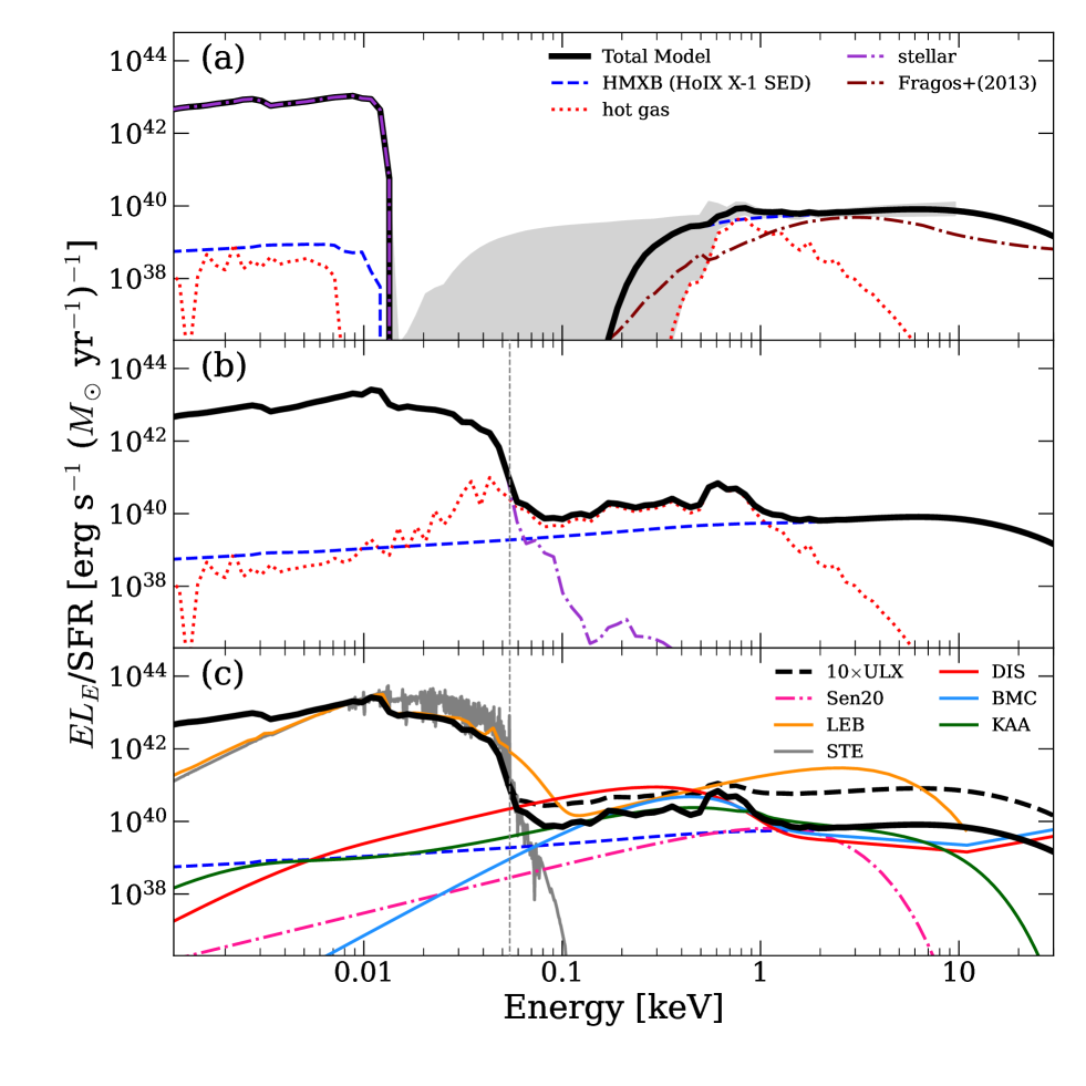
Figure 9: Broad band ($E=$ 0.001–30 keV; $\lambda=$ 0.4–12,400 Å) SFR-normalized model SEDs for our full sample. We display both the “observed” ($a$) and “intrinsic” ($b$ and $c$) SED models. The observed SED model consists of contributions from stellar, nebular, and dust emission (dot-dashed lavendar curve), along with attenuated emission from hot gas (dotted red curve) and HMXBs (dashed blue curve) (see § 6.3 for details). The gray shaded region surrounding the total observed model represents the 16–84% confidence range for the best-fit models. We note that these uncertainties are expected to be underestimated in the EUV (0.01–0.5 keV), where no data are present. For comparison, we show that the Fragos et al. (2013b) XRB models for $Z\approx 0.3Z_{\_}\odot$ galaxies (dot-dashed maroon curve) compare well with our HMXB SED constraint. The Fragos et al. (2013b) model has been used in assessing the impact of X-ray emission on the IGM in the high-redshift Universe (e.g., Das et al., 2017). The intrinsic SED model consists of the stellar emission, without nebular or dust absorption and emission, plus the unattenuated hot gas and HMXB emission (see panel $b$). In panel $c$, we show the intrinsic model compared with other SEDs in the literature. These include, the model for XRBs from Senchyna et al. (2020) (Sen20) at $L_{\_}{\rm X}$/SFR $=10^{40}$ erg s^-1, and various SEDs presented in Simmonds et al. (2021) (see annotations and discussion in § 6.3.2 for details). Statistical fluctuations of the ULX populations in dwarf galaxies are common and could lead to elevated $L_{\_}{\rm X}$/SFR values (e.g., the dashed black curve representing a factor of 10 enhanced ULX rate) that could yield high levels of ionizing radiation sufficient to power He II emission.

6.3.2 The Intrinsic SED

Turning now to the intrinsic SED, the EUV and soft-X-ray components of the spectrum provide a measure of the ionizing photon budget for a variety of atomic species, including those that have been observed in nebulae, but are not readily produced by stellar populations (e.g., He II, C IV, O IV, and Ne V). As discussed in §1, He II nebular emission, in particular, has been studied extensively in the literature, and its connection to X-ray emitting sources is under debate. For example, Schaerer et al. (2019) showed that the intensity of the high-ionization He II $\lambda$4686 line, relative to H$\beta$ $\lambda$4861, correlates with metallicity, following a similar relation to the $L_{\_}{\rm X}$(HMXB)-SFR-$Z$ plane, thus implicating HMXBs as a potential source of the He II ionization. In an attempt to extrapolate HMXB spectral models into the EUV, Senchyna et al. (2020, hereafter, Sen20) used multicolor accretion disk models to show HMXBs would fall short of producing the requisite levels of ionizing photons needed to power He II $\lambda$4686 in low-metallicity galaxies, unless $L_{\_}{\rm X}$/SFR $\lower 2.15277pt\hbox{$\;\buildrel>\over{\sim}\;$}10^{42}$ erg s^-1, a value that is $\approx$100 times that observed for typical galaxies. Also, it has been noted that the spatial extent of He II $\lambda$4686 and X-ray emission do not always coincide (e.g., Kehrig et al., 2021), arguing against a direct causal connection. However, in more recent works it has been argued that the extrapolations into the EUV from Sen20 are likely to be unrealistic for fits to actual ULXs (e.g., Simmonds et al., 2021, hereafter, Sim21; see below), and the effects of ULX beaming may not yield direct spatial coincidence between ULXs and the nebulae that they irradiate (Rickards Vaught et al., 2021).

In Figures 9$b$ and 9$c$, we show our intrinsic SED model, after the removal of obscuration and nebular/dust emission from our observed models. From Figure 9$b$, our extrapolation suggests that the EUV flux is dominated by X-ray emission from hot gas, with significant contributions from stellar emission near the He II ionization potential at 0.054 keV (denoted as a vertical line). For our adopted model, the HMXB (or ULX) contribution is a factor of $\approx$2–10 times below that of the hot gas across the EUV range. However, it is important to note that the HMXB versus hot gas normalization ratio is highly uncertain and subject to large galaxy-to-galaxy statistical fluctuations, especially for galaxies with low SFRs, due to stochastic sampling of the HMXB XLF and variations in ULX spectra. Stochastic fluctuations are expected to be amplified with decreasing metallicity as the bright end of the HMXB XLF flattens (see, e.g., §5.1 of L21 for details). As such, the relative ULX-to-hot-gas components could easily fluctuate by an order of magnitude or more for galaxies with SFR $\lower 2.15277pt\hbox{$\;\buildrel<\over{\sim}\;$}0.1$ $M_{\odot}$ yr^-1, and HMXBs (ULXs, in particular) may indeed play an important role in the overall EUV photon budget.

To provide context to our constraint, in Figure 9$c$ we have overlaid the SED of Sen20 (magenta dash-dot curve) normalized to a value of $L_{\_}{\rm X}$(HMXB)/SFR = $10^{40}$ erg s^-1 ($M_{\odot}$ yr^-1)^-1, comparable to the average value of our sample. For a fixed $L_{\_}{\rm X}$(HMXB)/SFR, extrapolation of the Sen20 curve results in a factor of $\approx$10–100 times lower intensity than our model produce from 0.054–0.5 keV where He II ionizing photons are important. If we boost the $L_{\_}{\rm X}$(HMXB)/SFR value of our model by a factor of 10, while holding the hot gas component fixed (see dashed curve in Figure 9$c$), the ionizing photon rate would consistently exceed the Sen20 rate by a factor of $\approx$100 across the EUV. Such a large positive fluctuation in $L_{\_}{\rm X}$(HMXB)/SFR to just above $10^{41}$ erg s^-1 ($M_{\odot}$ yr^-1)^-1 is readily observed in dwarf galaxies, and is comparable to that observed for I Zw 18, which has been studied extensively for its He II emission signatures (e.g., Kehrig et al., 2021; Rickards Vaught et al., 2021).

For further comparison, we have displayed in Figure 9$c$ the SED models considered by Sim21, who evaluated the impact of various ULX model extrapolations on high-ionization nebular emission lines He II $\lambda$4686 and [Ne V] $\lambda$3426. Three of the Sim21 models include a stellar component of age 1 Myr, based on BPASS models (“STE”) that is combined with three ULX models, including: (1) an accretion disk irradiated by an inner corona (“DIS”; Gierliński et al., 2009; Berghea & Dudik, 2012); (2) thermal photons produced in the inner region of an accretion disk that are Comptonized by material undergoing relativistic bulk motion (“BMC”; Titarchuk et al., 1997; Berghea & Dudik, 2012); and (3) a Comptonization model (Poutanen & Svensson, 1996) with a multicolor accretion disk that was used to fit NGC 5408 X-1, a ULX surrounded by a He II nebula (“KAA”; Kaaret & Corbel, 2009). In addition to these three ULX-based models, Sim21 analyze the optical–to–X-ray SED model presented in Lebouteiller et al. (2017, “LEB”;), which includes the combination of stellar plus accretion disk components that successfully model the observed optical and X-ray spectra of I Zw 18 and provide the requisite ionizing flux to power the observed He II emission in that galaxy.

For the three ULX models, Sim21 varied the ratio of intrinsic $L_{\_}{\rm X}^{\rm int}$/SFR (where SFR is estimated using the 1500 Å luminosity) and used photoionization modeling to show that He II $\lambda$4686 and [Ne V] $\lambda$3426 could be produced at the observed levels for values $L_{\_}{\rm X}^{\rm int}$/SFR $\lower 2.15277pt\hbox{$\;\buildrel>\over{\sim}\;$}10^{40}$ erg s^-1 ($M_{\odot}$ yr^-1)^-1 for the DIS model and $L_{\_}{\rm X}^{\rm int}$/SFR $\;\buildrel>\over{\sim}\;$ $3\times 10^{40}$ erg s^-1 ($M_{\odot}$ yr^-1)^-1 for the BMC and KAA models. For illustrative purposes, the Sim21 models displayed in Figure 9$c$ have been normalized to $L_{\_}{\rm X}^{\rm int}$/SFR $=3\times 10^{40}$ erg s^-1 ($M_{\odot}$ yr^-1)^-1  a level that is sufficient to power the He II. These models produce comparable levels of ionizing photons in the EUV and similar values of observed $L_{\_}{\rm X}$/SFR (i.e., $\beta_{\_}{\rm HMXB}$) to our nominal model. Furthermore, we find that observed statistical fluctuations of $\beta_{\_}{\rm HMXB}$ that are a factor of $\approx$10 above the average value can produce enhanced levels of ionizing emission over those of the Sim21 BCM and KAA models with $L_{\_}{\rm X}^{\rm int}$/SFR $=3\times 10^{40}$ erg s^-1 ($M_{\odot}$ yr^-1)^-1. Given the large uncertainties in extrapolating to the EUV, it is therefore not possible to exclude X-ray emitting sources as potentially important sources of producing these high-ionization emission lines.

7 Summary

We have combined UV–to–IR data and new Chandra observations of a sample of relatively low metallicity ($Z\approx 0.3Z_{\_}\odot$) star-forming galaxies, located at $D\approx$ 200–450 Mpc, to characterize the population average 0.5–8 keV spectral shape and normalization per SFR. We spectrally disentangled the relative HMXB and hot gas emission components of the spectrum and evaluated how $L_{\_}{\rm X}$/SFR for both components in these low-metallicity galaxies compares with more typical (and higher metallicity) populations in the nearby Universe. Our findings are summarized as follows:

1. Our $Z\approx 0.3Z_{\_}\odot$ galaxy sample was constructed to have relatively high SFR values (0.5–15 $M_{\odot}$ yr^-1) and low stellar masses ($\log M_{\_}\star/M_{\_}\odot=$ 8.0–9.3) with very high sSFRs (3–9 Gyr^-1) to ensure the X-ray emitting populations are dominated by HMXBs and hot gas, which are associated with young star-formation. As such, our sample is biased towards young stellar ages, and the HMXB populations may be associated with populations that are younger and more luminous than those presented in the literature with similar galaxy metallicities.

2. Chandra observations were conducted to obtain sufficient X-ray counts for constraining the sample-average 0.5–8 keV spectral shape. The relatively large size of our sample, compared to past studies of low-metallicity galaxies, minimizes the expected effects of stochastic variations on the average scaling relation.

3. Using the full Chandra data set, we constructed a global SFR-scaled spectral model that consisted of an absorbed two-temperature plasma (hot gas) with $kT\approx 0.2$ and 0.7 keV plus an absorbed power-law component (HMXBs) with photon index $\Gamma\approx 1.8$. Our global model provides a statistically acceptable description of the Chandra spectral data set, taken as a whole, with the majority of the galaxies being well fit on an individual basis. We identify only a single potential AGN (J101815.1+462623.9), which contains an excess of counts over our model near 6–7 keV, plausibly indicating the presence of a heavily-obscured/Compton-thick AGN.

4. Our global model provides a means for extracting scaling relations between SFR and the X-ray emission from hot gas and HMXBs separately. We find that the SFR-scaled HMXB X-ray luminosity (i.e., $L_{\_}{\rm 0.5-8~{}keV}^{\rm HMXB}$/SFR) is elevated for our $Z\approx 0.3Z_{\_}\odot$ galaxies compared with higher-metallicity galaxy samples. Specifically, we find $L_{\_}{\rm 0.5-8~{}keV}^{\rm HMXB}$/SFR $=40.19\pm 0.06$, which is $\approx$4 times higher than the solar-metallicity scaling relation. This value is also somewhat elevated (by a factor of $\approx$1.2–1.5) compared with extrapolated $L_{\_}{\rm X}$-SFR-$Z$ relations in the literature, which we speculate may be due to our sample having relatively low intrinsic HMXB obscuration and elevated HMXB emission from relatively young and X-ray-luminous HMXB populations.

5. For the hot gas component, we find a SFR scaling of $L_{\_}{\rm 0.5-2~{}keV}^{\rm gas}$/SFR = $39.58_{\_}{-0.28}^{+0.17}$ for our low-metallicity sample. We use our constraints, along with measurements from local galaxies with comparable SFR values (Mineo et al., 2012a), to show that $L_{\_}{\rm 0.5-2~{}keV}^{\rm gas}$/SFR declines with metallicity. The level of this trend is consistent with increased soft X-ray absorption from metal lines and edges with increasing metal abundances for a fixed hydrogen column density. However, this trend is only weakly constrained, and more detailed studies are required to both verify the trend and uncover its physical nature.

6. Using our X-ray global model, along with stellar, nebular, and dust emission and absorption models of the UV–to–IR data, we construct both emergent (observed) and intrinsic IR–to–X-ray SFR-scaled SED models. We show that by making reasonable interpolations into the EUV, our constraints on low-metallicity galaxy emergent emission are consistent with recent HERA constraints on X-ray emission from high-redshift galaxies, which are expected to contain low-metallicity galaxies. We also find that our intrinsic SED model produces significant EUV emission, and with modest fluctuations in the ULX population luminosity, which are commonly observed in dwarf galaxies, the EUV emission can exceed that required to power observed He II nebulae.

Acknowledgements: We thank the anonymous referee for their helpful comments on the manuscript. We thank Charlotte Simmonds for kindly providing spectral energy distribution models to compare with our results. We gratefully acknowledge financial support from Chandra X-ray Center (CXC) grant GO0-2J076A (B.D.L., R.T.E., A.B.) and NASA Astrophysics Data Analysis Program 80NSSC20K0444 (B.D.L.,R.T.E.). Some of the material is based upon work supported by NASA under award number 80GSFC21M0002 (A.B.). K.G. acknowledges support by the NASA Postdoctoral Program at Goddard Space Flight Center, administered by Oak Ridge Associated Universities under contract with NASA. A.M. gratefully acknowledges support by the European Research Council (ERC) under the European Union’s Horizon 2020 research and innovation programme (grant agreement No 638809 – AIDA). The results presented here reflect the authors’ views; the ERC is not responsible for their use.

This research has made use of the NASA/IPAC Extragalactic Database (NED), which is operated by the Jet Propulsion Laboratory, California Institute of Technology, under contract with the National Aeronautics and Space Administration.

References

- 2MASS Team (2020) 2MASS Team. 2020, 2MASS All-Sky Atlas Image Service, IPAC, doi: 10.26131/IRSA121
- Aird et al. (2017) Aird, J., Coil, A. L., & Georgakakis, A. 2017, MNRAS, 465, 3390, doi: 10.1093/mnras/stw2932
- Alam et al. (2015) Alam, S., Albareti, F. D., Allende Prieto, C., et al. 2015, ApJS, 219, 12, doi: 10.1088/0067-0049/219/1/12
- Andrieu & Thoms (2008) Andrieu, C., & Thoms, J. 2008, Statistics and Computing, 18, 343, doi: 10.1007/s11222-008-9110-y
- Arnaud (1996) Arnaud, K. A. 1996, in Astronomical Society of the Pacific Conference Series, Vol. 101, Astronomical Data Analysis Software and Systems V, ed. G. H. Jacoby & J. Barnes, 17
- Bartalucci et al. (2014) Bartalucci, I., Mazzotta, P., Bourdin, H., & Vikhlinin, A. 2014, A&A, 566, A25, doi: 10.1051/0004-6361/201423443
- Basu-Zych et al. (2016) Basu-Zych, A. R., Lehmer, B., Fragos, T., et al. 2016, ApJ, 818, 140, doi: 10.3847/0004-637X/818/2/140
- Basu-Zych et al. (2013a) Basu-Zych, A. R., Lehmer, B. D., Hornschemeier, A. E., et al. 2013a, ApJ, 762, 45, doi: 10.1088/0004-637X/762/1/45
- Basu-Zych et al. (2013b) —. 2013b, ApJ, 774, 152, doi: 10.1088/0004-637X/774/2/152
- Bayliss et al. (2020) Bayliss, M. B., McDonald, M., Sharon, K., et al. 2020, Nature Astronomy, 4, 159, doi: 10.1038/s41550-019-0888-7
- Berg et al. (2021) Berg, D. A., Chisholm, J., Erb, D. K., et al. 2021, ApJ, 922, 170, doi: 10.3847/1538-4357/ac141b
- Berghea & Dudik (2012) Berghea, C. T., & Dudik, R. P. 2012, ApJ, 751, 104, doi: 10.1088/0004-637X/751/2/104
- Bluem et al. (2019) Bluem, J., Kaaret, P., Prestwich, A., & Brorby, M. 2019, MNRAS, 487, 4093, doi: 10.1093/mnras/stz1574
- Bonamente (2019) Bonamente, M. 2019, arXiv e-prints, arXiv:1912.05444. https://arxiv.org/abs/1912.05444
- Brorby & Kaaret (2017) Brorby, M., & Kaaret, P. 2017, MNRAS, 470, 606, doi: 10.1093/mnras/stx1286
- Brorby et al. (2016) Brorby, M., Kaaret, P., Prestwich, A., & Mirabel, I. F. 2016, MNRAS, 457, 4081, doi: 10.1093/mnras/stw284
- Burke et al. (2021) Burke, D., Laurino, O., wmclaugh, et al. 2021, sherpa/sherpa: Sherpa 4.13.0, 4.13.0, Zenodo, doi: 10.5281/zenodo.4428938
- Calzetti et al. (2000) Calzetti, D., Armus, L., Bohlin, R. C., et al. 2000, ApJ, 533, 682, doi: 10.1086/308692
- Cash (1979) Cash, W. 1979, ApJ, 228, 939, doi: 10.1086/156922
- Chabrier (2003) Chabrier, G. 2003, PASP, 115, 763, doi: 10.1086/376392
- Chambers et al. (2016) Chambers, K. C., Magnier, E. A., Metcalfe, N., et al. 2016, arXiv e-prints, arXiv:1612.05560. https://arxiv.org/abs/1612.05560
- Crowther et al. (2016) Crowther, P. A., Caballero-Nieves, S. M., Bostroem, K. A., et al. 2016, MNRAS, 458, 624, doi: 10.1093/mnras/stw273
- Das et al. (2017) Das, A., Mesinger, A., Pallottini, A., Ferrara, A., & Wise, J. H. 2017, MNRAS, 469, 1166, doi: 10.1093/mnras/stx943
- Dittenber et al. (2020) Dittenber, B., Oey, M. S., Hodges-Kluck, E., et al. 2020, ApJL, 890, L12, doi: 10.3847/2041-8213/ab723e
- Doore et al. (2021) Doore, K., Eufrasio, R. T., Lehmer, B. D., et al. 2021, ApJ, 923, 26, doi: 10.3847/1538-4357/ac25f3
- Douna et al. (2015) Douna, V. M., Pellizza, L. J., Mirabel, I. F., & Pedrosa, S. E. 2015, A&A, 579, A44, doi: 10.1051/0004-6361/201525617
- Draine & Li (2007) Draine, B. T., & Li, A. 2007, ApJ, 657, 810, doi: 10.1086/511055
- Eide et al. (2020) Eide, M. B., Ciardi, B., Graziani, L., et al. 2020, MNRAS, 498, 6083, doi: 10.1093/mnras/staa2774
- Eldridge et al. (2017) Eldridge, J. J., Stanway, E. R., Xiao, L., et al. 2017, PASA, 34, e058, doi: 10.1017/pasa.2017.51
- Eufrasio et al. (2017) Eufrasio, R. T., Lehmer, B. D., Zezas, A., et al. 2017, ApJ, 851, 10, doi: 10.3847/1538-4357/aa9569
- Fabbiano (1989) Fabbiano, G. 1989, ARA&A, 27, 87, doi: 10.1146/annurev.aa.27.090189.000511
- Fabbiano (2006) —. 2006, ARA&A, 44, 323, doi: 10.1146/annurev.astro.44.051905.092519
- Fabbiano (2019) —. 2019, X-Rays from Galaxies, ed. B. Wilkes & W. Tucker, 7–1, doi: 10.1088/2514-3433/ab43dcch7
- Fioc & Rocca-Volmerange (1997) Fioc, M., & Rocca-Volmerange, B. 1997, A&A, 326, 950. https://arxiv.org/abs/astro-ph/9707017
- Fornasini et al. (2020) Fornasini, F. M., Civano, F., & Suh, H. 2020, MNRAS, 495, 771, doi: 10.1093/mnras/staa1211
- Fornasini et al. (2019) Fornasini, F. M., Kriek, M., Sanders, R. L., et al. 2019, ApJ, 885, 65, doi: 10.3847/1538-4357/ab4653
- Fragos et al. (2013a) Fragos, T., Lehmer, B. D., Naoz, S., Zezas, A., & Basu-Zych, A. 2013a, ApJL, 776, L31, doi: 10.1088/2041-8205/776/2/L31
- Fragos et al. (2008) Fragos, T., Kalogera, V., Belczynski, K., et al. 2008, ApJ, 683, 346, doi: 10.1086/588456
- Fragos et al. (2013b) Fragos, T., Lehmer, B., Tremmel, M., et al. 2013b, ApJ, 764, 41, doi: 10.1088/0004-637X/764/1/41
- Franeck et al. (2022) Franeck, A., Wünsch, R., Martínez-González, S., et al. 2022, arXiv e-prints, arXiv:2201.12339. https://arxiv.org/abs/2201.12339
- Fruscione et al. (2006) Fruscione, A., McDowell, J. C., Allen, G. E., et al. 2006, in Society of Photo-Optical Instrumentation Engineers (SPIE) Conference Series, Vol. 6270, Society of Photo-Optical Instrumentation Engineers (SPIE) Conference Series, ed. D. R. Silva & R. E. Doxsey, 62701V, doi: 10.1117/12.671760
- Garofali et al. (2020) Garofali, K., Lehmer, B. D., Basu-Zych, A., et al. 2020, ApJ, 903, 79, doi: 10.3847/1538-4357/abba2d
- Gelman et al. (1996) Gelman, A., Roberts, G., & Gilks, W. 1996, Statistica Sinica, 6, 733. www.jstor.org/stable/24306036
- Gierliński et al. (2009) Gierliński, M., Done, C., & Page, K. 2009, MNRAS, 392, 1106, doi: 10.1111/j.1365-2966.2008.14166.x
- Gilbertson et al. (2021) Gilbertson, W., Lehmer, B., Doore, K., et al. 2021, arXiv e-prints, arXiv:2112.03194. https://arxiv.org/abs/2112.03194
- Gilfanov et al. (2004) Gilfanov, M., Grimm, H. J., & Sunyaev, R. 2004, MNRAS, 351, 1365, doi: 10.1111/j.1365-2966.2004.07874.x
- Grimes et al. (2005) Grimes, J. P., Heckman, T., Strickland, D., & Ptak, A. 2005, ApJ, 628, 187, doi: 10.1086/430692
- Grimm et al. (2003) Grimm, H. J., Gilfanov, M., & Sunyaev, R. 2003, MNRAS, 339, 793, doi: 10.1046/j.1365-8711.2003.06224.x
- Gross et al. (2021) Gross, A. C., Prestwich, A., & Kaaret, P. 2021, MNRAS, 505, 610, doi: 10.1093/mnras/stab1331
- Guo et al. (2010) Guo, Q., White, S., Li, C., & Boylan-Kolchin, M. 2010, MNRAS, 404, 1111, doi: 10.1111/j.1365-2966.2010.16341.x
- Hao et al. (2011) Hao, C.-N., Kennicutt, R. C., Johnson, B. D., et al. 2011, ApJ, 741, 124, doi: 10.1088/0004-637X/741/2/124
- Hastings (1970) Hastings, W. K. 1970, Biometrika, 57, 97, doi: 10.1093/biomet/57.1.97
- Heneka & Mesinger (2020) Heneka, C., & Mesinger, A. 2020, MNRAS, 496, 581, doi: 10.1093/mnras/staa1517
- Jaskot & Oey (2013) Jaskot, A. E., & Oey, M. S. 2013, ApJ, 766, 91, doi: 10.1088/0004-637X/766/2/91
- Joye & Mandel (2003) Joye, W. A., & Mandel, E. 2003, in Astronomical Society of the Pacific Conference Series, Vol. 295, Astronomical Data Analysis Software and Systems XII, ed. H. E. Payne, R. I. Jedrzejewski, & R. N. Hook, 489
- Justham & Schawinski (2012) Justham, S., & Schawinski, K. 2012, MNRAS, 423, 1641, doi: 10.1111/j.1365-2966.2012.20985.x
- Kaaret & Corbel (2009) Kaaret, P., & Corbel, S. 2009, ApJ, 697, 950, doi: 10.1088/0004-637X/697/1/950
- Kaastra (2017) Kaastra, J. S. 2017, A&A, 605, A51, doi: 10.1051/0004-6361/201629319
- Kehrig et al. (2021) Kehrig, C., Guerrero, M. A., Vílchez, J. M., & Ramos-Larios, G. 2021, ApJL, 908, L54, doi: 10.3847/2041-8213/abe41b
- Kennicutt (1998) Kennicutt, Robert C., J. 1998, ApJ, 498, 541, doi: 10.1086/305588
- Kewley & Ellison (2008) Kewley, L. J., & Ellison, S. L. 2008, ApJ, 681, 1183, doi: 10.1086/587500
- Kouroumpatzakis et al. (2020) Kouroumpatzakis, K., Zezas, A., Sell, P., et al. 2020, MNRAS, 494, 5967, doi: 10.1093/mnras/staa1063
- Kovlakas et al. (2020) Kovlakas, K., Zezas, A., Andrews, J. J., et al. 2020, MNRAS, 498, 4790, doi: 10.1093/mnras/staa2481
- Kroupa (2001) Kroupa, P. 2001, MNRAS, 322, 231, doi: 10.1046/j.1365-8711.2001.04022.x
- Kuntz & Snowden (2010) Kuntz, K. D., & Snowden, S. L. 2010, ApJS, 188, 46, doi: 10.1088/0067-0049/188/1/46
- Lebouteiller et al. (2017) Lebouteiller, V., Péquignot, D., Cormier, D., et al. 2017, A&A, 602, A45, doi: 10.1051/0004-6361/201629675
- Lehmer et al. (2010) Lehmer, B. D., Alexander, D. M., Bauer, F. E., et al. 2010, ApJ, 724, 559, doi: 10.1088/0004-637X/724/1/559
- Lehmer et al. (2008) Lehmer, B. D., Brandt, W. N., Alexander, D. M., et al. 2008, ApJ, 681, 1163, doi: 10.1086/588459
- Lehmer et al. (2015) Lehmer, B. D., Tyler, J. B., Hornschemeier, A. E., et al. 2015, ApJ, 806, 126, doi: 10.1088/0004-637X/806/1/126
- Lehmer et al. (2016) Lehmer, B. D., Basu-Zych, A. R., Mineo, S., et al. 2016, ApJ, 825, 7, doi: 10.3847/0004-637X/825/1/7
- Lehmer et al. (2019) Lehmer, B. D., Eufrasio, R. T., Tzanavaris, P., et al. 2019, ApJS, 243, 3, doi: 10.3847/1538-4365/ab22a8
- Lehmer et al. (2021) Lehmer, B. D., Eufrasio, R. T., Basu-Zych, A., et al. 2021, ApJ, 907, 17, doi: 10.3847/1538-4357/abcec1
- Li & Wang (2013a) Li, J.-T., & Wang, Q. D. 2013a, MNRAS, 428, 2085, doi: 10.1093/mnras/sts183
- Li & Wang (2013b) —. 2013b, MNRAS, 435, 3071, doi: 10.1093/mnras/stt1501
- Linden et al. (2010) Linden, T., Kalogera, V., Sepinsky, J. F., et al. 2010, ApJ, 725, 1984, doi: 10.1088/0004-637X/725/2/1984
- Lopez et al. (2020) Lopez, L. A., Mathur, S., Nguyen, D. D., Thompson, T. A., & Olivier, G. M. 2020, ApJ, 904, 152, doi: 10.3847/1538-4357/abc010
- Madau & Fragos (2017) Madau, P., & Fragos, T. 2017, ApJ, 840, 39, doi: 10.3847/1538-4357/aa6af9
- Mainali et al. (2017) Mainali, R., Kollmeier, J. A., Stark, D. P., et al. 2017, ApJL, 836, L14, doi: 10.3847/2041-8213/836/1/L14
- Mainali et al. (2018) Mainali, R., Zitrin, A., Stark, D. P., et al. 2018, MNRAS, 479, 1180, doi: 10.1093/mnras/sty1640
- McQuinn et al. (2018) McQuinn, K. B. W., Skillman, E. D., Heilman, T. N., Mitchell, N. P., & Kelley, T. 2018, MNRAS, 477, 3164, doi: 10.1093/mnras/sty839
- Mesinger et al. (2013) Mesinger, A., Ferrara, A., & Spiegel, D. S. 2013, MNRAS, 431, 621, doi: 10.1093/mnras/stt198
- Mineo et al. (2014) Mineo, S., Gilfanov, M., Lehmer, B. D., Morrison, G. E., & Sunyaev, R. 2014, MNRAS, 437, 1698, doi: 10.1093/mnras/stt1999
- Mineo et al. (2012a) Mineo, S., Gilfanov, M., & Sunyaev, R. 2012a, MNRAS, 426, 1870, doi: 10.1111/j.1365-2966.2012.21831.x
- Mineo et al. (2012b) —. 2012b, MNRAS, 419, 2095, doi: 10.1111/j.1365-2966.2011.19862.x
- Mirabel et al. (2011) Mirabel, I. F., Dijkstra, M., Laurent, P., Loeb, A., & Pritchard, J. R. 2011, A&A, 528, A149, doi: 10.1051/0004-6361/201016357
- Morrissey et al. (2007) Morrissey, P., Conrow, T., Barlow, T. A., et al. 2007, ApJS, 173, 682, doi: 10.1086/520512
- Olivier et al. (2021) Olivier, G. M., Berg, D. A., Chisholm, J., et al. 2021, arXiv e-prints, arXiv:2109.06725. https://arxiv.org/abs/2109.06725
- Owen & Warwick (2009) Owen, R. A., & Warwick, R. S. 2009, MNRAS, 394, 1741, doi: 10.1111/j.1365-2966.2009.14464.x
- Pacucci et al. (2014) Pacucci, F., Mesinger, A., Mineo, S., & Ferrara, A. 2014, MNRAS, 443, 678, doi: 10.1093/mnras/stu1240
- Pakull & Angebault (1986) Pakull, M. W., & Angebault, L. P. 1986, Nature, 322, 511, doi: 10.1038/322511a0
- Park et al. (2019) Park, J., Mesinger, A., Greig, B., & Gillet, N. 2019, MNRAS, 484, 933, doi: 10.1093/mnras/stz032
- Persic & Rephaeli (2007) Persic, M., & Rephaeli, Y. 2007, A&A, 463, 481, doi: 10.1051/0004-6361:20054146
- Pettini & Pagel (2004) Pettini, M., & Pagel, B. E. J. 2004, MNRAS, 348, L59, doi: 10.1111/j.1365-2966.2004.07591.x
- Poutanen & Svensson (1996) Poutanen, J., & Svensson, R. 1996, ApJ, 470, 249, doi: 10.1086/177865
- Prestwich et al. (2013) Prestwich, A. H., Tsantaki, M., Zezas, A., et al. 2013, ApJ, 769, 92, doi: 10.1088/0004-637X/769/2/92
- Ranalli et al. (2003) Ranalli, P., Comastri, A., & Setti, G. 2003, A&A, 399, 39, doi: 10.1051/0004-6361:20021600
- Rickards Vaught et al. (2021) Rickards Vaught, R. J., Sandstrom, K. M., & Hunt, L. K. 2021, ApJL, 911, L17, doi: 10.3847/2041-8213/abf09b
- Salim et al. (2016) Salim, S., Lee, J. C., Janowiecki, S., et al. 2016, ApJS, 227, 2, doi: 10.3847/0067-0049/227/1/2
- Salmon et al. (2015) Salmon, B., Papovich, C., Finkelstein, S. L., et al. 2015, ApJ, 799, 183, doi: 10.1088/0004-637X/799/2/183
- Saxena et al. (2020) Saxena, A., Pentericci, L., Schaerer, D., et al. 2020, MNRAS, 496, 3796, doi: 10.1093/mnras/staa1805
- Saxena et al. (2021) Saxena, A., Ellis, R. S., Forster, P. U., et al. 2021, arXiv e-prints, arXiv:2104.02624. https://arxiv.org/abs/2104.02624
- Schaerer (1996) Schaerer, D. 1996, ApJL, 467, L17, doi: 10.1086/310193
- Schaerer et al. (2019) Schaerer, D., Fragos, T., & Izotov, Y. I. 2019, A&A, 622, L10, doi: 10.1051/0004-6361/201935005
- Senchyna et al. (2019) Senchyna, P., Stark, D. P., Chevallard, J., et al. 2019, MNRAS, 488, 3492, doi: 10.1093/mnras/stz1907
- Senchyna et al. (2020) Senchyna, P., Stark, D. P., Mirocha, J., et al. 2020, MNRAS, 494, 941, doi: 10.1093/mnras/staa586
- Shirazi & Brinchmann (2012) Shirazi, M., & Brinchmann, J. 2012, MNRAS, 421, 1043, doi: 10.1111/j.1365-2966.2012.20439.x
- Simmonds et al. (2021) Simmonds, C., Schaerer, D., & Verhamme, A. 2021, arXiv e-prints, arXiv:2108.12438. https://arxiv.org/abs/2108.12438
- Smith et al. (2018) Smith, B. J., Campbell, K., Struck, C., et al. 2018, AJ, 155, 81, doi: 10.3847/1538-3881/aaa1a6
- Smith et al. (2019) Smith, B. J., Wagstaff, P., Struck, C., et al. 2019, AJ, 158, 169, doi: 10.3847/1538-3881/ab3e72
- Song et al. (2016) Song, M., Finkelstein, S. L., Ashby, M. L. N., et al. 2016, ApJ, 825, 5, doi: 10.3847/0004-637X/825/1/5
- Spergel et al. (2003) Spergel, D. N., Verde, L., Peiris, H. V., et al. 2003, ApJS, 148, 175, doi: 10.1086/377226
- Stanway & Eldridge (2018) Stanway, E. R., & Eldridge, J. J. 2018, MNRAS, 479, 75, doi: 10.1093/mnras/sty1353
- Stark et al. (2017) Stark, D. P., Ellis, R. S., Charlot, S., et al. 2017, MNRAS, 464, 469, doi: 10.1093/mnras/stw2233
- Stefanon et al. (2021) Stefanon, M., Bouwens, R. J., Labbé, I., et al. 2021, ApJ, 922, 29, doi: 10.3847/1538-4357/ac1bb6
- Strickland et al. (2004) Strickland, D. K., Heckman, T. M., Colbert, E. J. M., Hoopes, C. G., & Weaver, K. A. 2004, ApJS, 151, 193, doi: 10.1086/382214
- Strickland & Stevens (2000) Strickland, D. K., & Stevens, I. R. 2000, MNRAS, 314, 511, doi: 10.1046/j.1365-8711.2000.03391.x
- Svoboda et al. (2019) Svoboda, J., Douna, V., Orlitová, I., & Ehle, M. 2019, ApJ, 880, 144, doi: 10.3847/1538-4357/ab2b39
- Symeonidis et al. (2014) Symeonidis, M., Georgakakis, A., Page, M. J., et al. 2014, MNRAS, 443, 3728, doi: 10.1093/mnras/stu1441
- The HERA Collaboration et al. (2021) The HERA Collaboration, Abdurashidova, Z., Aguirre, J. E., et al. 2021, arXiv e-prints, arXiv:2108.07282. https://arxiv.org/abs/2108.07282
- Thuan et al. (2004) Thuan, T. X., Bauer, F. E., Papaderos, P., & Izotov, Y. I. 2004, ApJ, 606, 213, doi: 10.1086/382949
- Titarchuk et al. (1997) Titarchuk, L., Mastichiadis, A., & Kylafis, N. D. 1997, ApJ, 487, 834, doi: 10.1086/304617
- Tyler et al. (2004) Tyler, K., Quillen, A. C., LaPage, A., & Rieke, G. H. 2004, ApJ, 610, 213, doi: 10.1086/421544
- Vito et al. (2016) Vito, F., Gilli, R., Vignali, C., et al. 2016, MNRAS, 463, 348, doi: 10.1093/mnras/stw1998
- Vulic et al. (2021) Vulic, N., Hornschemeier, A. E., Haberl, F., et al. 2021, arXiv e-prints, arXiv:2106.14526. https://arxiv.org/abs/2106.14526
- Walton et al. (2017) Walton, D. J., Fürst, F., Harrison, F. A., et al. 2017, ApJ, 839, 105, doi: 10.3847/1538-4357/aa683e
- Walton et al. (2018) Walton, D. J., Fürst, F., Heida, M., et al. 2018, ApJ, 856, 128, doi: 10.3847/1538-4357/aab610
- Wang et al. (2021) Wang, Q. D., Zeng, Y., Bogda, A., & Ji, L. 2021, arXiv e-prints, arXiv:2110.06995. https://arxiv.org/abs/2110.06995
- Waters et al. (2020) Waters, C. Z., Magnier, E. A., Price, P. A., et al. 2020, ApJS, 251, 4, doi: 10.3847/1538-4365/abb82b
- Wiktorowicz et al. (2017) Wiktorowicz, G., Sobolewska, M., Lasota, J.-P., & Belczynski, K. 2017, ApJ, 846, 17, doi: 10.3847/1538-4357/aa821d
- WISE Team (2020) WISE Team. 2020, AllWISE Atlas (L3a) Coadd Images, IPAC, doi: 10.26131/IRSA153