Parallel framework for Dynamic Domain Decomposition of Data Assimilation problems

Abstract

[Abstract]We focus on PDE-based Data Assimilation problems (DA) solved by means of variational approaches and Kalman Filter algorithm. Recently, we presented a Domain Decomposition framework (we call it DD-DA, for short) performing a decomposition of the whole physical domain along space and time directions, and joining the idea of Schwarz’s methods and Parallel in Time (PinT)- based approaches. For effective parallelization of domain decomposition algorithms, the computational load assigned to sub domains must be equally distributed. Usually computational cost is proportional to the amount of data entities assigned to partitions. Good quality partitioning also requires the volume of communication during calculation to be kept at its minimum. In order to deal with DD-DA problems where the observations are non uniformly distributed and general sparse, in the present work we employ a parallel load balancing algorithm - based on adaptive and dynamic defining of boundaries of DD - which is aimed to balance workload according to data location. We call it DyDD. As the numerical model underlying DA problems arising from the so-called discretize-then-optimize approach is the Constrained Least Square model (CLS), we will use CLS as a reference state estimation problem and we validate DyDD on different scenarios.

1 Introduction

Data Assimilation (DA, for short) encompasses the entire sequence of operations that, starting from observations/measurements of physical quantities and from additional information - such as a mathematical model governing the evolution of these quantities - improve their estimate minimizing inherent uncertainties. DA problems are usually formulated as an optimization problem where the objective function measures the mismatch between the model predictions and the observed system states, weighted by the inverse of the error covariance matrices^{12, 34}. In operational DA the amount of observations is insufficient to fully describe the system and one cannot strongly rely on a data driven approach: the model is paramount. It is the model that fills the spatial and temporal gaps in the observational network: it propagates information from observed to unobserved areas. Thus, DA methods are designed to achieve the best possible use of a never sufficient (albeit constantly growing) amount of data, and to attain an efficient data model fusion, in a short period of time. This poses a formidable computational challenge, and makes DA an example of big data inverse problems^{3, 4, 5, 14}. There is a lot of DA algorithms. Two main approaches gained acceptance as powerful methods: variational approach (namely 3DVAR and 4DVAR) and Kalman Filter (KF) ^{24, 29, 37}. Variational approaches are based on the minimization of the objective function estimating the discrepancy between numerical results and observations. These approaches assume that the two sources of information, forecast and observations, have errors that are adequately described by stationary error covariances. In contrast to variational methods, KF (and its variants) is a recursive filter solving the Euler-Lagrange equations. It uses a dynamic error covariance estimate evolving over a given time interval. The process is sequential, meaning that observations are assimilated in chronological order, and KF alternates a forecast step, when the covariance is evolved, with an analysis step in which covariance of the filtering conditional is updated. In both kind of methods the model is integrated forward in time and the result is used to reinitialize the model before the integration continues. For any details interested readers are referred to³⁰.
Main operators of any DA algorithm are dynamic model and observation mapping. These are two main components of any variational approach and state estimation problem, too. In this regard, in the following, as proof of concept of the DyDD framework, we start considering CLS model, seen as a prototype of Data Assimilation model ²⁶. CLS is obtained combining two overdetermined linear systems, representing the state and the observation mapping, respectively. In this regards, in ¹⁵ we presented a feaibility analysis on Constrained Least Square (CLS) models of an innovative Domain Decomposition (DD) framework for using CLS in large scale applications. DD framework, based on Schwarz approach, that properly combines localization and PDE-based model reduction inheriting the advantages of both techniques for effectively solving any kind of large scale and/or real time KF application. It involves decomposition of the physical domain, partitioning of the solution, filter localization and model reduction, both in space and in time. There is a quite different rationale behind the DD framework and the so called Model Order Reduction methods (MOR) ³⁶, even though they are closely related each other. The primary motivation of Schwarz based DD methods was the inherent parallelism arising from a flexible, adaptive and independent decomposition of the given problem into several subproblems, though they can also reduce the complexity of sequential solvers. Schwarz Methods and theoretical frameworks are, to date, the most mature for this class of problems ^{20, 26, 38}. MOR techniques are based on projection of the full order model onto a lower dimensional space spanned by a reduced order basis. These methods has been used extensively in a variety of fields for efficient simulations of highly intensive computational problems. But all numerical issues concerning the quality of approximation still are of paramount importance ²⁸. As mentioned previously DD-DA framework makes it natural to switch from a full scale solver to a model order reduction solver for solution of subproblems for which no relevant low-dimensional reduced space should be constructed. In the same way, DD-DA framework allows to employ a model reduction in space and time which is coherent with the filter localization. In conclusion, main advantage of the DD framework is to combine in the same theoretical framework model reduction, along the space and time directions, with filter localization, while providing a flexible, adaptive, reliable and robust decomposition. That said, any interest reader who wants to apply DD framework in a real-world application, i.e. with a (PDE-based) model state and an observation mapping, once the dynamic (PDE-based) model state has been discretized, he should rewrite the state estimation problem under consideration as a CLS model problem (cfr Section 3.1) and then to apply DD algorithm. In other words, she/he should follow the discretize-then-optmize approach, common to most Data Assimilation problems and state estimation problems, before employing the DD framework. Summarizing, main topics of DD framework can be listed as follows.

1. DD step: we begin by partitioning along space and time the domain into subdomains and then extending each subdomain to overlap its neighbors by an amount. Partitioning can be adapted according to the availability of measurements and data.

2. Filter Localization and MOR: on each subdomain we formulate a local DA problem analogous to the original one, combining filter localization and model order reduction approaches.

3. Regularization constraints: in order to enforce the matching of local solutions on the overlapping regions, local DA problems are slightly modified by adding a correction term. Such a correction term balances localization errors and computational efforts, acting as a regularization constraint on local solutions. This is a typical approach for solving ill posed inverse problems (see for instance 33).

4. Parallel in Time: as the dynamic model is coupled with DA operator, at each integration step we employ, as initial and boundary values of all reduced models, estimates provided by the DA model itself, as soon as these are available.

5. Conditioning: localization excludes remote observations from each analyzed location, thereby improving the conditioning of the error covariance matrices. To the best of our knowledge, such ab-initio space and time decomposition of DA models has never been investigated before. A spatially distributed KF into sensor based reduced-order models, implemented on a sensor networks where multiple sensors are mounted on a robot platform for target tracking, is presented in ^{6, 31}.

1.1 Contribution of the present work

In this work we focus on the introduction of a dynamic redefining of the DD, aimed to efficiently deal with DA problems where observations are non uniformly distributed and general sparse. Indeed, in such cases a static and/or a-priori DD strategy could not ensure a well balanced workload, while a way to re-partition the domain so that subdomains maintain a nearly equal number of observations plays an essential role in the success of any effective DD approach. We present a revision of DD framework such that a dynamic load balancing algorithm allows for a minimal data movement restricted to the neighboring processors. This is achieved by considering a connected graph induced by the domain partitioning whose vertices represent a subdomain associated with a scalar representing the number of observations on that sub domain. Once the domain has been partitioned, a load balancing schedule (scheduling step) should make the load on each subdomain equals to the average load providing the amount of load to be sent to adjacent subdomains (migrations step). The most intensive kernel is the scheduling step which defines a schedule for computing the load imbalance (which we quantify in terms of number of observations) among neighbouring subdomains. Such quantity is then used to update the shifting the adjacent boundaries of sub domains (Migration step) which are finally re mapped to achieve a balanced decomposition. We are assuming that load balancing is restricted to the neighbouring domains so that we reduce the overhead processing time. Finally, following ¹⁸ we use a diffusion type scheduling algorithm minimizing the euclidean norm of data movement. The resulting constrained optimization problem leads to normal equations whose matrix is associated to the decomposition graph. The disadvantage is that the overhead time, due to the final balance between sub domains, strongly depends on the degree of the vertices of processors graph, i.e. on the number of neighbouring subdomains for each subdomain. Such overhead represents the surface-to-volume ratio whose impact on the overall performance of the parallel algorithm decreases as the problem size increases.

1.2 Related Works

There has been widespread interests in load balancing since the introduction of large scale multiprocessors. Applications requiring dynamic load balancing mainly include parallel solution of a partial differential equation (PDE) by finite elements on an unstructured grids ¹⁶ or parallelized particle simulations ¹⁹. Load balancing is one of the central problems which have to be solved in designing parallel algorithms. Moreover, problems whose workload changes during the computation or it depends on data layout which may be unknown a priori, will necessitate the redistribution of the data in order to retain efficiency. Such a strategy is known as dynamic load balancing. Algorithms for dynamic load balancing, as in ^{11, 7, 39, 40}, are based on transferring an amount of work among processors to neighbours; the process is iterated until the load difference between any two processors is smaller than a specified value, consequently it will not provide a balanced solution immediately. A multilevel diffusion method for dynamic load balancing ¹⁷, is based on bisection of processor graph. The disadvantage is that, to ensure the connectivity of subgraphs, movement of data between non-neighbouring processors can occur. The mentioned algorithms do not take into account one important factor, namely that the data movement resulting from the load balancing schedule should be kept to minimum.

1.2.1 Organization of the work

The present work is organized as follows. As we apply the proposed framework to CLS model which can be seen as prototype of variational DA models, in order to improve the readability of the article, in Section §2 we give a brief overview of DA methods, i.e. both Kalman Filter and Variational DA, the variational formulation of KF and finally we give a brief description of CLS model. In Section §3 we describe main features of DD framework and its application to CLS model. DyDD is presented in Section §4, through a graphical description and the numerical algorithm. Validation and performance results are presented in Section §5 and, finally, in Section §6 we give conclusions and future works.

2 The Background

In order to improve the readability of the article, in this section we give a brief overview of DA methods, i.e. both Kalman Filter and Variational DA, then we review CLS model as prototype of DA models. To this end, we also review the variational formulation of KF, i.e. the so-called VAR–KF formulation, obtained minimizing the sum of the weighted Euclidean norm of the model error and the weighted Euclidean norm of the observation error.

2.1 Kalman Filter (KF)

Given $x_{0}\in\mathbb{R}^{n}$, let $x(t)\in\mathbb{R}^{n}$, $\forall t\in[0,T]$, denote the state of a dynamic system governed by the mathematical model $\mathcal{M}_{t,t+\Delta t}[x(t)]$, $\Delta t>0$:

$$\left\{\begin{array}[]{ll}x(t+\Delta t)&=\mathcal{M}_{t,t+\Delta t}(x(t)),\ \ \forall t,t+\Delta t\in[0,T]\\ x(0)&=x_{0}\end{array},\right.$$ (1)

and let:

$$y(t+\Delta t)=\mathcal{H}_{t+\Delta t}[x(t+\Delta t)],$$ (2)

denote the observations where $\mathcal{H}_{t+\Delta t}$ is the observations mapping. Chosen $r\in\mathbb{N}$, we consider $r+2$ points in $[0,T]$ and $\Delta t=\frac{T}{r+1}$.
Let $\{t_{k}\}_{k=0,1,\ldots,r+1}$ be a discretization of $[0,T]$, where $t_{k}=k\Delta t$, and let $\widehat{x}_{k}$ be the state estimate at time $t_{k}$, for $k=1,...,r+1$; we will use the following operators ³⁷: , for $k=0,1,...,r$, $M_{k,k+1}\in\mathbb{R}^{n\times n}$, denoting the discretization of a linear approximation of $\mathcal{M}_{t_{k},t_{k+1}}$ and for $k=0,1,...,r+1$, $H_{k}\in\mathbb{R}^{m\times n}$ which is the discretization of a linear approximation of $\mathcal{H}_{t}$ with $m>n$. Moreover, we let $w_{k}\in\mathbb{R}^{n}$ and $v_{k}\in\mathbb{R}^{m}$ be model and observation errors with normal distribution and zero mean such that $E[w_{k}v_{i}^{T}]=0$, for $i,k=0,1,...,r+1$, where $E[\cdot]$ denotes the expected value; $Q_{k}\in\mathbb{R}^{n\times n}$ and $R_{k}\in\mathbb{R}^{m\times m}$, are covariance matrices of the errors on the model and on the observations, respectively i.e.

$$Q_{k}:=E[w_{k}w_{k}^{T}]\quad R_{k}:=E[v_{k}v_{k}^{T}]\quad\textit{$\forall$ $k=0,1,...,r+1$}.$$

These matrices are symmetric and positive definite.

KF method: KF method consists in calculating the estimate $\widehat{x}_{k+1}$, at time $t_{k+1}$, of the state $x_{k+1}\in\mathbb{R}^{n}$:

$$x_{k+1}=M_{k,k+1}x_{k}+w_{k},\quad\textit{$\forall k=0,1,...,r$}$$ (3)

such that

$$y_{k+1}=H_{k+1}{x}_{k+1}+v_{k+1},\quad\textit{$\forall k=0,1,...,r$}.$$ (4)

KF algorithm: Given $\widehat{x}_{0}\in\mathbb{R}^{n}$ and $P_{0}=O\in\mathbb{R}^{n\times n}$ a null matrix, for each $k=0,1,\ldots,r$ KF algorithm is made by two main operations: the Predicted phase, consisting of the computation of the predicted state estimate:

$$x_{k+1}=M_{k,k+1}\widehat{x}_{k};$$ (5)

and of the predicted error covariance matrix:

$$P_{k+1}=M_{k,k+1}P_{k}M_{k,k+1}^{T}+Q_{k};$$ (6)

and the Corrector phase, consisting of the computation of Kalman gain:

$$K_{k+1}=P_{k+1}H_{k+1}^{T}(H_{k+1}P_{k+1}H_{k+1}^{T}+R_{k+1})^{-1},$$ (7)

of Kalman covariance matrix:

$$P_{k+1}=(I-K_{k+1}H_{k+1})P_{k+1},$$

and of Kalman state estimate:

$$\widehat{x}_{k+1}=x_{k+1}+K_{k+1}(y_{k+1}-H_{k+1}x_{k+1}).$$ (8)

Finally, we introduce the VAR-KF model. For $k=0,1,\ldots,r$:

$$\begin{array}[]{ll}\widehat{x}_{k+1}&=argmin_{x_{k+1}\in\mathbb{R}^{n}}J_{k+1}(x_{k+1})\\ &=argmin_{x_{k+1}\in\mathbb{R}^{n}}\left\{||x_{k+1}-M_{k,k+1}\widehat{x}_{k}||_{Q_{k}}^{2}+||y_{k+1}-H_{k+1}{x}_{k+1}||_{R_{k+1}}^{2}\right\}.\end{array}$$

3 VAR DA model Set Up

If $\Omega\subset\mathbb{R}^{n}$, $n\in\mathbb{N}$, is a spatial domain with a Lipschitz boundary, let:

$$\left\{\begin{array}[]{ll}u(t+h,x)=\mathcal{M}_{t,t+h}[u(t,x)]&\textrm{$\forall x\in\Omega$, $t,t+h\in[0,T]$, $(h>0)$}\\ u(t_{0},x)=u_{0}(x)&\textrm{$t_{0}\equiv 0,\ \ x\in\Omega$}\\ u(t,x)=f(x)&\textrm{$x\in\partial\Omega$, $\forall t\in[0,T]$}\\ \end{array},\right.$$ (9)

be a symbolic description of the 4D–DA model of interest where

$$u:(t,x)\in[0,T]\times\Omega\mapsto u(t,x)=[u[1](t,x),u[2](t,x),\ldots,u[pv](t,x)],$$

is the state function of $\mathcal{M}$ with $pv\in\mathbb{N}$ the number of physical variables, $f$ is a known function defined on the boundary $\partial\Omega$, and let

$$v:(t,x)\in[0,T]\times\Omega\mapsto v(t,x),$$

be the observations function, and

$$\mathcal{H}:u(t,x)\mapsto v(t,x),\ \ \ \ \ \forall(t,x)\in[0,T]\times\Omega,$$

denote the non-linear observations mapping. To simplify future treatments we assume $pv\equiv 1$. We consider $N_{p}$ points of $\Omega\subset\mathbb{R}^{n}$ $:$ $\{x_{j}\}_{j=1,\ldots,N_{p}}\subset\Omega$; $n_{obs}$ points of $\Omega$, where $n_{obs}<<N_{p}$, $:$ $\{y_{j}\}_{j=1,\ldots,n_{obs}}$; $N$ points of [0,T] $:$ $D([0,T])=\{t_{l}\}_{l=0,1,\ldots,N-1}$ with $t_{l}=t_{0}+l(hT)$; the vector

$$u_{0}=\{u_{0,j}\}_{j=1,\ldots,N_{p}}\equiv\{u_{0}(x_{j})\}_{j=1,\ldots,N_{p}}\in\mathbb{R}^{N_{p}},$$

which is the state at time $t_{0}$; the operator

$$M_{l-1,l}\in\mathbb{R}^{N_{p}\times N_{p}},\ \ \ l=1,\ldots,N,$$

representing a discretization of a linear approximation of $\mathcal{M}_{t_{l-1},t_{l}}$ from $t_{l-1}$ to $t_{l}$; the vector $b\in\mathbb{R}^{N_{p}}$ accounting boundary conditions; the vector

$$u^{b}:=\{u_{l,j}^{b}\}_{l=1,\ldots,N-1;j=1,\ldots,N_{p}}\equiv\{u^{b}(t_{l},x_{j})\}_{l=1,\ldots,N-1;j=1,\ldots,N_{p}}\in\mathbb{R}^{N_{p}\cdot(N-1)},$$

representing solution of $M_{l-1,l}$ at $t_{l}$ for $l=1,\ldots,N$, i.e. the background; the vector

$$v_{l}\equiv\{v(t_{l},y_{j})\}_{j=1,\ldots,n_{obs}}\in\mathbb{R}^{l\cdot n_{obs}},$$

consisting of observations at $t_{l}$, for $l=0,\ldots,N-1$; the linear operator

$$H_{l}\in\mathbb{R}^{n_{obs}\times N_{p}},\ \ \ l=0,\ldots,N-1,$$

representing a linear approximation of $\mathcal{H}$; matrix $G\equiv G_{N-1}\in\mathbb{R}^{(N\cdot n_{obs})\times N_{p}}$ such that

$$G_{l}=\left\{\begin{array}[]{ll}\left[\begin{array}[]{ll}H_{0}\\ H_{1}\\ \vdots\\ H_{l-1}\end{array}\right]&\textrm{$l>1$}\\ \\ H_{0}&\textrm{$l=1$}\end{array},\right.$$

and $\textbf{R}=diag(\textbf{R}_{0},\textbf{R}_{1},\ldots,\textbf{R}_{N-1})$ and Q$=\textbf{V}\textbf{V}^{T}$, covariance matrices of the errors on observations and background, respectively. We now define the 4D–DA inverse problem ³³.

Definition 3.1.

(The 4D-DA inverse problem). Given the vectors $v=\{v_{l}\}_{l=0,\ldots,N-1}\in\mathbb{R}^{N\cdot n_{obs}},\ \ u_{0}\in\mathbb{R}^{N_{p}},$ and the block matrix $G\in\mathbb{R}^{(N\cdot n_{obs})\times N_{p}},$ a 4D–DA problem concerns the computation of

$$u^{DA}\in\mathbb{R}^{N_{p}},$$

such that

$$v=G\cdot u^{DA},$$ (10)

subject to the constraint that $u_{0}^{DA}=u_{0}.$

We also introduce the regularized 4D-DA inverse problem, i.e. the 4D–VAR DA problem.

Definition 3.2.

(The 4D–VAR DA problem). The 4D–VAR DA problem concerns the computation of:

$$u^{DA}=argmin_{u\in\mathbb{R}^{N_{p}}}J(u),$$ (11)

with

$$J(u)=\alpha||u-u^{b}||_{\textbf{Q}^{-1}}^{2}+||Gu-v||_{\textbf{R}^{-1}}^{2},$$ (12)

where $\alpha$ is the regularization parameter.

Remark: It is worth noting that here we are considering a linear approximation of the observation operator, hence a linear operator $G$, although this is not at all required, at least in the formulation of the 4D–VAR problem. A more general approach for numerically linearize and solve 4D–VAR DA problem consists in defining a sequence of local approximations of $\mathbf{J}$ where each member of the sequence is minimized by employing Newton’s method or one its variants. More precisely, two approaches could be employed:

1. by truncating Taylor’s series expansion of $\mathbf{J}$ at the second order, giving a quadratic approximation of $\mathbf{J}$, let us say $\mathbf{J}^{QN}$. Newton’methods (including LBFGS and Levenberg-Marquardt) use $\mathbf{J}^{QD}$. The minimum is computed solving the linear system involving the Hessian matrix $\nabla^{2}\mathbf{{J}}$, and the negative gradient $-\nabla\mathbf{{J}}$.

2. by truncating Taylor’s series expansion of $\mathbf{J}$ at the first order which gives a linear approximation of $\mathbf{J}$, let us say let us say $\mathbf{J}^{TL}$. Gauss-Newton’s methods (including Truncated or Approximated Gauss-Newton uses $\mathbf{J}^{TL}$). The minimum is computed solving the normal equations arising from the local Linear Least Squares problem.

Both approaches will employ the Tangent Linear Model (TLM) and the adjoint operator of the observation mapping and of the model of interest ⁹.

Remark: Computational kernel of variational approaches (namely 3D-Var and 4D-Var) is a linear system, generally solved by means of iterative methods; the iteration matrix is related to matrix Q, which usually has a Gaussian correlation structure ¹⁴. Matrix Q can be written in the form Q$=\textbf{V}\textbf{V}^{T}$, where V is the square root of Q, namely it is a Gaussian matrix. As a consequence, products of V and a vector z are Gaussian convolutions which can be efficiently computed by applying Gaussian recursive filters as in ¹³.
In our case study we carry out on CLS model, we apply KF and DD-KF to CLS model, then in this case it results that matrix Q is the null matrix while matrix R is diagonal ¹⁵.

3.1 Constrained Least Squares (CLS) Problem

Let

$$H_{0}x_{0}=y_{0},\quad H_{0}\in\mathbb{R}^{m_{0}\times n},\quad y_{0}\in\mathbb{R}^{m_{0}},\quad x_{0}\in\mathbb{R}^{n}$$ (13)

be the overdetermined linear system (the state), where $rank(H_{0})=n>0$, $m_{0}>n$.
Given $H_{1}\in\mathbb{R}^{m_{1}\times n}$, $y_{1}\in\mathbb{R}^{m_{1}}$, $x_{1}\in\mathbb{R}^{n}$, $x\in\mathbb{R}^{n}$ (the observations), we consider the system

$$S:\ \ Ax=b$$ (14)

where

$$A=\left[\begin{array}[]{llll}H_{0}\\ H_{1}\\ \end{array}\right]\in\mathbb{R}^{(m_{0}+m_{1})\times n},\quad b=\left[\begin{array}[]{llll}y_{0}\\ y_{1}\\ \end{array}\right]\in\mathbb{R}^{m_{0}+m_{1}},$$ (15)

and $m_{1}>0$. Let $R_{0}\in\mathbb{R}^{m_{0}\times m_{0}}$, $R_{1}\in\mathbb{R}^{m_{1}\times m_{1}}$ be weight matrices and $R=diag(R_{0},R_{1})\in\mathbb{R}^{(m_{0}+m_{1})\times(m_{0}+m_{1})}$.
CLS problem consists in the computation of $\widehat{x}$ such that:

$$CLS:\ \ \widehat{x}=argmin_{x\in\mathbb{R}^{n}}J(x)$$ (16)

with

$$\begin{array}[]{ll}J(x)=||Ax-b||_{R}^{2}=||H_{0}x-y_{0}||_{{R}_{0}}^{2}+||H_{1}x-y_{1}||_{{R}_{1}}^{2},\end{array}$$ (17)

where $\widehat{x}$ is given by

$$(A^{T}RA)\widehat{x}=A^{T}Rb\Rightarrow\ \widehat{x}=(A^{T}RA)^{-1}A^{T}Rb$$ (18)

or,

$$\widehat{x}=(H_{0}^{T}R_{0}H_{0}+H_{1}^{T}R_{1}H_{1})^{-1}(H_{0}^{T}R_{0}y_{0}+H_{1}^{T}R_{1}y_{1}).$$ (19)

We refer to $\widehat{x}$ as solution in least squares sense of system in (14).

Remark: Besides covariance matrices of errors, main components of KF algorithm are dynamic model and observation mapping. These are two main components of any variational Data Assimilation operator and state estimation problem, too. In this regard, in the following, as proof of concept of DD framework, we start considering CLS model as a prototype of a variational Data Assimilation model, at a given time. CLS is obtained combining two overdetermined linear systems, representing the state and the observation mapping, respectively. Then, we introduce VAR-KF method as reference data sampling method solving CLS model problem. VAR-KF will be decomposed by using the proposed DD framework. That said, any interest reader who wants to apply DD framework in a real-world application, i.e. with a (PDE-based) model state and an observation mapping, once the dynamic (PDE-based) model state has been discretized, he should rewrite the state estimation problem under consideration as a CLS model problem (cfr Section 3.1) and then to apply CLS algorithm. In other words, she/he should follow the discretize-then-optmize approach, common to most Data Assimilation problems and state estimation problems, before employing DyDD framework.

4 DD-framework

As DyDD is the refinement of initial DD, in the following we first give mathematical settings useful to define the domain decomposition framework. Then, in next section we focus on DyDD.

4.1 DD set up

Definition 4.1.

(Matrix Reduction) Let $B=[B^{1}\ B^{2}\ \dots\ B^{n}]\in\mathbb{R}^{m\times n}$ be a matrix with $m,n\geq 1$ and $B^{j}$ the $j-th$ column of $B$ and $I_{j}=\{1,\dots,j\}$ and $I_{i,j}=\{i,\dots,j\}$ for $i=1,\dots,n-1$; $j=2,\dots,n$, and $i<j$ for every $(i,j)$. Reduction of $B$ to $I_{j}$ is:

$$|_{I_{j}}:\ B\in\mathbb{R}^{m\times n}\rightarrow\ B|_{I_{j}}=[B^{1}\ B^{2}\ \dots\ B^{j}]\in\mathbb{R}^{m\times j},\quad\textit{ $j=2,\dots,n$},$$

and to $I_{i,j}$

$$|_{I_{i,j}}:\ B\in\mathbb{R}^{m\times n}\rightarrow\ B|_{I_{i,j}}=[B^{i}\ B^{i+1}\ \dots\ B^{j}]\in\mathbb{R}^{m\times j-i},\quad\textit{ $i=1,\dots,n-1$, $j>i$},$$

where $B|_{I_{j}}$ and $B|_{I_{i,j}}$ denote reduction of $B$ to $I_{j}$ and $I_{i,j}$, respectively.

Definition 4.2.

(Vector Reduction) Let $w=[w_{t}\ w_{t+1}\ \dots\ w_{n}]^{T}\in\mathbb{R}^{s}$ be a vector with $t\geq 1$, $n>0$, $s=n-t$ and $I_{1,r}=\{1,\dots,r\}$, $r>n$ and $n>t$. The extension of $w$ to $I_{r}$ is:

$$EO_{I_{r}}:\ w\in\mathbb{R}^{s}\rightarrow\ EO_{I_{r}}(w)=[\bar{w}_{1}\ \bar{w}_{2}\ \dots\ \bar{w}_{r}]^{T}\in\mathbb{R}^{r},$$

where $i=1,\ldots,r$

$$\bar{w}_{i}=\left\{\begin{array}[]{ll}w_{i}&\textit{if $t\leq i\leq n$}\\ 0&\textit{if $i>n$ and $i<t$}\\ \end{array}\right.\quad.$$

We introduce reduction of $J$, as given in (17).

Definition 4.3.

(Model Reduction) Let us consider $A\in\mathbb{R}^{(m_{0}+m_{1})\times n}$, $b\in\mathbb{R}^{m_{0}+m_{1}}$, the matrix and the vector defined in (15), $I_{1}=\{1,\ldots,n_{1}\}$, $I_{2}=\{1,\ldots,n_{2}\}$ with $n_{1},n_{2}>0$ and the vectors $x\in\mathbb{R}^{n}$. Let

$$J|_{(I_{i},I_{j})}:(x|_{I_{i}},x|_{I_{j}})\longmapsto J|_{(I_{i},I_{j})}(x|_{I_{i}},x|_{I_{j}})\quad\textit{$\forall i,j=1,2$}$$

denote the reduction of $J$ defined in (17). It is defined as

$$J|_{(I_{i},I_{j})}(x|_{I_{i}},x|_{I_{j}})=||H_{0}|_{I_{i}}x|_{I_{i}}-(y_{0}+H_{0}|_{I_{j}}x|_{I_{j}})||_{R_{0}}^{2}+||H_{1}|_{I_{i}}x|_{I_{i}}-(y_{1}+H_{1}|_{I_{j}}x|_{I_{j}})||_{R_{1}}^{2},$$ (20)

for $i,j=1,2$.

For simplicity of notations we let $J_{i,j}\equiv J|_{(I_{i},I_{j})}$.

4.2 DD-CLS problems: DD of CLS model

We apply DD approach for solving system $S$ in (14). Here, for simplicity of notations, we consider two subdomains.

Definition 4.4.

(DD-CLS model¹⁵) Let $S$ be the overdetermined linear system in (14) and $A\in\mathbb{R}^{(m_{0}+m_{1})\times n}$, $b\in\mathbb{R}^{m_{0}+m_{1}}$ the matrix and the vector defined in (15) and ${R}_{0}\in\mathbb{R}^{m_{0}\times m_{0}}$, ${R}_{1}\in\mathbb{R}^{m_{1}\times m_{1}}$, $R=diag(R_{0},{R}_{1})\in\mathbb{R}^{(m_{0}+m_{1})\times(m_{0}+m_{1})}$ be the weight matrices with $m_{0}>n$ and $m_{1}>0$. Let us consider the index set of columns of $A$, $I=\{1,\dots,n\}$. DD-CLS model consists of:

• DD step. It consists of DD of $I$:

  $$I_{1}=\{1,\ldots,n_{1}\},\ \ \ I_{2}=\{n_{1}-s+1,\ldots,n\},$$ (21)

  where $s\geq 0$ is the number of indexes in common, $|I_{1}|=n_{1}>0$, $|I_{2}|=n_{2}>0$, and the overlap sets

  $${I}_{1,2}=\{{n}_{1}-s+1,\ldots,n_{1}\},$$ (22)

  If $s=0$, then $I$ is decomposed without using the overlap, i.e. $I_{1}\cap I_{2}=\emptyset$ and ${I}_{1,2}\neq\emptyset$, instead if $s>0$ i.e. $I$ is decomposed using overlap, i.e. $I_{1}\cap I_{2}\neq\emptyset$ and ${I}_{1,2}=\emptyset$; restrictions of $A$ to $I_{1}$ and $I_{2}$ defined in (21)

  $${A}_{1}=A|_{{I}_{1}}\in\mathbb{R}^{(m_{0}+m_{1})\times n_{1}},\quad{A}_{2}=A|_{{I}_{2}}\in\mathbb{R}^{(m_{0}+m_{1})\times n_{2}},$$ (23)

• DD-CLS step: given $x_{2}^{0}\in\mathbb{R}^{n_{2}}$, according to the ASM (Alternating Schwarz Method) in ²⁶, DD-CLS approach consists in solving for $n=0,1,2,\ldots$ the following overdetermined linear systems:

  $$S_{1}^{n+1}:\ \ {A}_{1}x_{1}^{n+1}={b}-A_{2}x_{2}^{n};\quad S_{2}^{n+1}:\ \ {A}_{2}x_{2}^{n+1}={b}-A_{1}x_{1}^{n+1},$$ (24)

  by employing a regularized VAR-KF model. It means that DD-CLS consists of a sequence of two subproblems:

  $$\begin{array}[]{ll}P_{1}^{n+1}:\ \widehat{x}_{1}^{n+1}&=argmin_{x_{1}^{n+1}\in\mathbb{R}^{n_{1}}}J_{1}(x_{1}^{n+1},x_{2}^{n})\\ &=argmin_{x_{1}^{n+1}\in\mathbb{R}^{n_{1}}}\left[J|_{(I_{1},I_{2})}(x_{1}^{n+1},x_{2}^{n})+\mu\cdot\mathcal{O}_{1,2}(x_{1}^{n+1},x_{2}^{n})\right]\end{array}$$ (25)

  $$\begin{array}[]{ll}P_{2}^{n+1}:\ \widehat{x}_{2}^{n+1}&=argmin_{x_{2}^{n+1}\in\mathbb{R}^{n_{2}}}J_{2}(x_{2}^{n+1},x_{1}^{n+1})\\ &=argmin_{x_{2}^{n+1}\in\mathbb{R}^{n_{2}}}\left[J|_{(I_{2},I_{1})}(x_{2}^{n+1},x_{1}^{n+1})+\mu\cdot\mathcal{O}_{1,2}(x_{2}^{n+1},x_{1}^{n+1})\right]\end{array}$$ (26)

  where ${I_{i}}$ is defined in (21) and $J|_{I_{i},I_{j}}$ is defined in (20), $\mathcal{O}_{1,2}$ is the overlapping operator and $\mu>0$ is the regularization parameter.

Remark 4.5.

If $I$ is decomposed without using overlap (i.e. $s=0$), then $\widehat{x}_{1}^{n+1}\in\mathbb{R}^{n_{1}}$ and $\widehat{x}_{2}^{n+1}\in\mathbb{R}^{n_{2}}$ can be written in terms of normal equations as follows

$$\begin{array}[]{ll}\tilde{S}_{1}^{n+1}:\ (A_{1}^{T}RA_{1})\widehat{x}_{1}^{n+1}=A_{1}^{T}R(b-A_{2}x_{2}^{n})&\Rightarrow\widehat{x}_{1}^{n+1}=(A_{1}^{T}RA_{1})^{-1}A_{1}^{T}Rb_{1}^{n}\\ \tilde{S}_{2}^{n+1}:\ (A_{2}^{T}RA_{2})\widehat{x}_{2}^{n+1}=A_{2}^{T}R(b-A_{1}x_{1}^{n+1})&\Rightarrow\widehat{x}_{2}^{n+1}=(A_{2}^{T}RA_{2})^{-1}A_{2}^{T}Rb_{2}^{n+1},\end{array}$$ (27)

where $b_{1}^{n}=b-A_{2}x_{2}^{n}$ and $b_{2}^{n+1}=b-A_{1}x_{1}^{n+1}$.

Remark 4.6.

Regarding the operator $\mathcal{O}_{1,2}$, we consider $x_{1}\in\mathbb{R}^{n_{1}}$ and $x_{2}\in\mathbb{R}^{n_{2}}$, and we pose

$$\mathcal{O}_{1,2}(x_{i},x_{j})=||EO_{I_{i}}({x}_{i}|_{{I}_{1,2}})-EO_{I_{i}}({{x}_{j}}|_{{I}_{1,2}})||,\ \textit{$i,j=1,2$}$$

with $EO_{I_{i}}({x}_{1}|_{I_{1,2}})$, $EO_{I_{i}}({x}_{2}|_{I_{1,2}})$ be the extension to $I_{i}$, of restriction to ${I}_{1,2}$ in (22) of $x_{1}\in\mathbb{R}^{n_{1}}$ and $x_{2}\in\mathbb{R}^{n_{2}}$, respectively. Operator $\mathcal{O}_{1,2}$ represents the exchange of data on the overlap $I_{1,2}$ in (22).

Remark 4.7.

DD-CLS gives to sequences $\{x^{n+1}\}_{n\in\mathbb{N}_{0}}$:

$$x^{n+1}=\left\{\begin{array}[]{ll}\widehat{x}_{1}^{n+1}|_{I_{1}\setminus I_{1,2}}&\textit{on $I_{1}\setminus I_{1,2}$}\\ \frac{\mu}{2}(\widehat{x}_{2}^{n+1}|_{I_{1,2}}+\widehat{x}_{1}^{n+1}|_{I_{1,2}})&\textit{on $I_{1,2}$}\\ \widehat{x}_{2}^{n+1}|_{I_{2}\setminus I_{1,2}}&\textit{on $I_{2}\setminus I_{1,2}$}\\ \end{array},\right.$$ (28)

where $I_{1}$, $I_{2}$ are defined in (21) and $I_{1,2}$ in (22).

Remark 4.8.

For DD-CLS model we considered, DD of $I=\{1,\ldots,n\}\subset\mathbb{N}$ i.e. the index set of columns of m $A$, similarly we can apply DD approach to 2D domain $I\times J\subset\mathbb{N}\times\mathbb{N}$, where $J=\{1,\ldots,(m_{0}+m_{1})\}$ is the rows index set of $A$. Sub domains obtained are $I_{1}\times J_{1}=\{1,\ldots,n_{1}\}\times\{1,\ldots,m^{1}\}$ and $I_{2}\times J_{2}=\{n_{1}-s_{I}+1,\ldots,n\}\times\{m^{1}-s_{J}+1,\ldots,(m_{0}+m_{1})\}$, where $s_{I},s_{J}\geq 0$ are the number of indexes in common between $I_{1}$ and $I_{2}$, $J_{1}$ and $J_{2}$, respectively. Restrictions of $A$ to $I_{1}\times J_{1}$ and $I_{2}\times J_{2}$ are $A_{1}:=A|_{I_{1}\times J_{1}}$ and $A_{2}:=A|_{I_{2}\times J_{2}}$.

Remark 4.9.

The cardinality of $J$, i.e. the index set of rows of matrix $A$, represents the number of observations available at time of the analysis, so that DD of $I\times J$ allows us to define DD-CLS model after dynamic load balancing of observations by appropriately restricting matrix $A$.

5 DyDD: Dynamic DD framework

For effective parallelization of DD based algorithms, domain partitioning into sub domains must satisfy certain conditions. Firstly the computational load assigned to sub domains must be equally distributed. Usually, computational cost is proportional to the amount of data entities assigned to partitions. Good quality partitioning also requires the volume of communication during calculation to be kept at its minimum. We employ a dynamic load balancing scheme based on adaptive and dynamic redefining of initial DD aimed to balance workload between processors. Redefining of initial partitioning is performed by shifting the boundaries of neighbouring domains (this step is referred to as Migration step).
DyDD algorithm we implement is described by procedure DyDD shown in Table 13. To the aim of giving a clear and immediate view of DyDD algorithm, in the following figures (Figures 1-4) we outline algorithm workout on a reference initial DD configuration made of eight subdomains. We assume that at each point of the mesh we have the value of numerical simulation result (the so called background) while the circles denote observations. DyDD framework consists in four steps:

1. DD step: starting from the initial partition of $\Omega$ provided by DD-DA framework, DyDD performs a check of the initial partitioning. If a subdomain is empty, it decomposes subdomain adjacent to that domain which has maximum load (decomposition is performed in $2$ subdomains). See Figure 1.

2. Scheduling step: DyDD computes the amount of observations needed for achieving the average load in each sub domain; this is performed by introducing a diffusion type algorithm (by using the connected graph G associated to the DD) derived by minimizing the Euclidean norm of the cost transfer. Solution of the laplacian system associated to the graph G gives the amount of data to migrate. See Figure 2.

3. Migration step: DyDD shifts the boundaries of adjacent sub domains to achieve a balanced workload. See Figure 3.

4. Update step: DyDD redefines subdomains such that each one contains the number of observations computed during the scheduling step and it redistributes subdomains among processors grids. See Figure 4.

Scheduling step is the computational kernel of DyDD algorithm. In particular, it requires definition of laplacian matrix and load imbalance associated to initial DD and its solution. Let us give a brief overview of this computation. Generic element $L_{ij}$ of laplacian matrix is defined as follows¹⁸:

$$L_{ij}=\left\{\begin{array}[]{ll}-1&i\neq j\,and\,edge\,(i,j)\in G\\ deg(i)&i=j,\\ 0&otherwise\end{array}\right.$$ (29)

and the load imbalance $b=\left(l\left(i\right)-\bar{l}\right)$, where $d\left(i\right)$ is the degree of vertex $i$, $l\left(i\right)$ and $\bar{l}$ are the number of observations and the average workload, respectively. Hence, as more edges are in G (as the number of subdomains which are adjacent to each other increases) as more non zero elements are in $L$.

Laplacian system $L\lambda=b$, related to the example described below, is the following:

$$L=\left[\begin{array}[]{ccccccccc}2&-1&-1&0&0&0&0&0\\ -1&3&-1&-1&0&0&0&0\\ -1&-1&4&-1&-1&0&0&0\\ 0&-1&-1&2&0&0&0&0\\ 0&0&-1&0&2&-1&0&0\\ 0&0&0&0&-1&3&-1&-1\\ 0&0&0&0&0&-1&2&-1&\\ 0&0&0&0&0&-1&-1&2&\\ \end{array}\right]$$ (30)

while the right hand side is the vector whose $i$-th component is given by the load imbalance, computed with respect to the average load. In this example, solution of the laplacian system gives

$$\lambda=(0.36,0.25,0.,1.12,-1.,-5.,-6.33,-6.67)$$

so that the amount of load (rounded to the nearest integer) which should be migrated from $\Omega_{i}$ to $\Omega_{j}$ is

$$\begin{array}[]{c}\delta_{1,2}=1;\delta_{1,3}=0;\delta_{3,2}=0;\delta_{3,4}=1;\delta_{3,5}=1;\delta_{5,6}=2;\delta_{6,7}=0;\delta_{6,8}=1;\delta_{7,8}=1.\end{array}$$

i.e. $\delta_{i,j}$ is the nearest integer of $(\lambda_{i}-\lambda_{j})$.

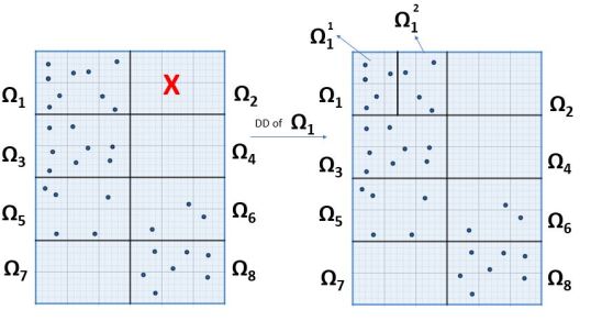
((a)) $\Omega_{1}$ is identified as having the maximum load w.r.t. its neighbourhoods.

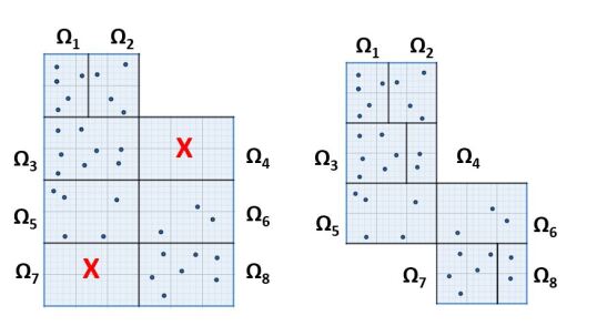
((b)) $\Omega_{4}$ and $\Omega_{7}$ are identified as having the maximum load w.r.t. their neighbourhoods.

Figure 1: DyDD framework - Step 1. Check of the initial partitioning, identification of subdomains which do not have data or they suffer of any load imbalance and redefinition of subdomains. We observe that the workload of each subdomain after this re-partitioning is now $l_{r}(1)=5$, $l_{r}(2)=4$, $l_{r}(3)=6$, $l_{r}(4)=2$, $l_{r}(5)=5$, $l_{r}(6)=3$, $l_{r}(7)=5$ and $l_{r}(8)=2.$ The average load is then $\bar{l}=4$.

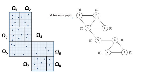
Figure 2: DyDD framework - Step 2. Scheduling. On the right, the graph G associated to the DD of $\Omega$. In brackets the number $l_{r}(i)$ is displayed.

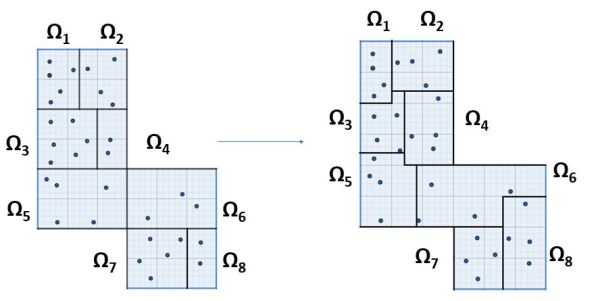
Figure 3: DyDD framework - Step 3. Migration. Redefinition of the boundaries of adjacent subdomains.

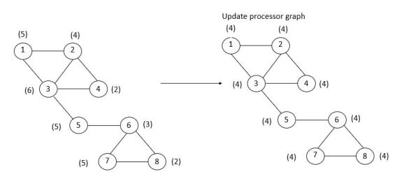
Figure 4: DyDD framework - Step 4. Update step. Updating of the processor graph. In brackets, the number of observations $l_{fi}(i)$ after DyDD is displayed. We observe that the workload of each subdomain after DyDD is equal to the average load $\bar{l}=4$.

6 Validation Results

Simulations were aimed to validate the proposed approach by measuring performance of DyDD algorithm. Performance evaluation was carried out using Parallel Computing Toolbox of MATLABR2013a on the High Performance hybrid Computing (HPC) architecture of the SCoPE (Sistema Cooperativo Per Elaborazioni scientifiche multidiscipliari) data center, located at University of Naples Federico II. More precisely, the HPC architecture is made of $8$ nodes, consisting of distributed memory DELL M600 blades connected by a $10$ Gigabit Ethernet technology. Each blade consists of $2$ Intel Xeon@2.33GHz quadcore processors sharing $16$ GB RAM memory for a total of 8 cores/blade and of $64$ cores, in total. In this case for testing the algorithm we consider up to $n_{sub}=64$ sub domains equally distributed among the cores. This is an intra-node configuration implementing a coarse-grained parallelization strategy on multiprocessor systems with many-core CPUs.

DyDD set up. We will refer to the following quantities: $\Omega\subset\mathbb{R}^{2}$: spatial domain; $n=2048$: mesh size; $m:$ number of observations; $p$: number of subdomains and processing units; $i$: identification number of processing unit, which is the same of the associated subdomain; for $i=1,\ldots,p$, $deg(i)$: degree of $i$, i.e. number of subdomains adjacent to $\Omega_{i}$; $i_{ad}(i)\in\mathbb{N}$: identification of subdomains adjacent to $\Omega_{i}$; $l_{in}(i)\in\mathbb{N}$: number of observations in $\Omega_{i}$ before the dynamic load balancing; $l_{r}(i)\in\mathbb{N}$: number of observations in $\Omega_{i}$ after DD step of DyDD procedure; $l_{fi}(i)\in\mathbb{N}$: number of observations in $\Omega_{i}$ after the dynamic load balancing; $T^{p}_{DyDD}(m)$: time (in seconds) needed to perform DyDD on $p$ processing units; $T_{r}(m)$: time (in seconds) needed to perform re-partitioning of $\Omega$; $Oh_{DyDD}(m)=\frac{T_{r}(m)}{T^{p}_{DyDD}(m)}$ overhead time to the dynamic load balancing. As measure of the load balance introduced by DyDD algorithm, we use:

$$\mathcal{E}=\frac{\min_{i}({l_{fi}(i)})}{\max_{i}({l_{fi}(i)})}\\$$

i.e. we compute the ratio of the minimum to the maximum of the number of observations of subdomains $\Omega_{1},\ldots,\Omega_{p}$ after DyDD, respectively. As a consequence, $\mathcal{E}$ = 1 indicates a perfectly balanced system.

Regarding DD-DA, we let $n_{loc}:=\frac{n}{p}$ be local problem size and we consider as performance metrics, the following quantities: $T^{1}\left(m,n\right)$ denoting sequential time (in seconds) to perform KF solving CLS problem; $T_{DD-DA}^{p}\left(m,n_{loc}\right)$ denoting time (in seconds) needed to perform in parallel DD-KF solving CLS problem after DyDD; $T_{oh}^{p}\left(m,n_{loc}\right)$ being the overhead time (measured in seconds) due to synchronization, memory accesses and communication time among $p$ cores; $\widehat{x}_{KF}\in\mathbb{R}^{n}$ denoting KF estimate obtained by applying the KF procedure on CLS problem after DyDD; $\widehat{x}_{DD-DA}\in\mathbb{R}^{n}$ denoting DD estimate obtained by applying DD-KF on CLS problem after DyDD; $error_{DD-DA}:=\|\widehat{x}_{KF}-\widehat{x}_{DD-DA}\|$ denoting the error introduced by the DD framework; $S^{p}\left(m,n_{loc}\right):=\frac{T^{1}\left(m,n\right)}{T_{DD-DA}^{p}(m,n_{loc})}$, which refers to the speed-up of DD-KF parallel algorithm; $E^{p}\left(m,n_{loc}\right):=\frac{S^{p}\left(m,n_{loc}\right)}{p}$ which denotes the efficiency of DD-KF parallel algorithm.

In the following tables we report results obtained by employing three scenarios, which are defined such that each one is gradually more articulated than the previous one. It means that the number of subdomains which are adjacent to each subdomain increases, or the number of observations and the number of subdomains increase. In this way the workload re distribution increases.

Example 1: First configuration: $p=2$ subdomains and $m=1500$ observations. In Case1, both $\Omega_{1}$ and $\Omega_{2}$ have data i.e. observations, but they are unbalanced. In Case2, $\Omega_{1}$ has observations and $\Omega_{2}$ is empty. In Table 1 and Table 2, respectively, we report values of the parameters after applying DyDD algorithm. This is the simplest configuration we consider just to validate DyDD framework. In both cases, $l_{fi}(1)$ and $l_{fi}(2)$, i.e. number of observations of $\Omega_{1}$ and $\Omega_{2}$, are equal to the average load $\bar{l}=750$ and $\mathcal{E}$ = 1. As the workload re distribution of Case 1 and Case 2 is the same, DD-KF performance results of Case 1 and Case 2 are the same, and they are reported in Table 9, for $p=2$ only. In Table 3 we report performance results of DyDD algorithm.

Table 1: Example 1. DyDD parameters in Case 1. Both subdomains have data but they are unbalanced. We report values of $p$, which is the number of subdomains, $i$ the identification number of processing unit, $deg(i)$ degree of $i$, i.e. number of subdomains adjacent to $\Omega_{i}$, $l_{in}(i)$ which is number of observations in $\Omega_{i}$ before dynamic load balancing, $l_{fi}(i)$ number of observations in $\Omega_{i}$ after dynamic load balancing, $i_{ad}$ identification of subdomains adjacent to $\Omega_{i}$.

p	$i$	$deg(i)$	${l_{in}}$	$l_{fin}$	$i_{ad}$
2	1	1	1000	750	2
	2	1	500	750	1

Table 2: Example 1. DyDD parameters in Case 2. $\Omega_{2}$ is empty. We report values of $p$ i.e. number of subdomains, $i$ identification number of processing unit, $deg(i)$ degree of $i$, i.e. number of subdomains adjacent to $\Omega_{i}$, $l_{in}(i)$ which is number of observations in $\Omega_{i}$ before dynamic load balancing, $l_{r}(i)$ number of observations in $\Omega_{i}$ after DD step of DyDD procedure, $l_{fi}(i)$ number of observations in $\Omega_{i}$ after dynamic load balancing, $i_{ad}$ which is identification of subdomains which are adjacent to $\Omega_{i}$.

p	$i$	$deg(i)$	$l_{in}$	$l_{r}$	$l_{fin}$	$i_{ad}$
2	1	1	1500	1000	750	2
	2	1	0	500	750	1

Table 3: Example 1. Execution times: we report values of $T^{p}_{DyDD}(m)$, time (in seconds) needed to perform DyDD on $p$ processing units, $T_{r}(m)$, time (in seconds) needed to perform re-partitioning of $\Omega$, $Oh_{DyDD}(m)$ overhead time due to dynamic load balancing and $\mathcal{E}$ measuring load balance.

Case	$T^{p}_{DyDD}(m)$	$T_{r}(m)$	$Oh_{DyDD}(m)$	$\mathcal{E}$
1	$4.11\times 10^{-2}$	0	0	1
2	$3.49\times 10^{-2}$	$4.00\times 10^{-6}$	$1.15\times 10^{-4}$	1

Example 2: Second configuration. In this experiment we consider $p=4$ subdomains and $m=1500$ observations, and four cases which are such that the number of subdomains not having observations, increases from $0$ up to $3$. In particular, in Case 1, all subdomains have observations. See Table 4. In Case 2, only one subdomain is empty, namely $\Omega_{2}$. See Table 5. In Case 3, two subdomains are empty, namely $\Omega_{1}$ and $\Omega_{2}$ are empty. See Table 6. In Case 4, three subdomains are empty, namely $\Omega_{j}$, for $j=1,2,3$, is empty. See Table 7. In all cases, $\mathcal{E}$ reaches the ideal value 1 and $l_{fin}(i)=\bar{l}=375$, $i=1,2,3,4$. Then, DD-KF performance results of all cases are the same and they are reported in Table 9 for $p=4$. In Table 8 we report performance results of the four cases.

Example 3. We consider $m=1032$ observations and a number of subdomains $p$ equals to $p=2,4,8,16,32$. We assume that all subdomains $\Omega_{i}$ has observations, i.e. for $i=1,\ldots,p$, $l_{in}(i)\neq 0$; $\Omega_{1}$ has $p-1$ adjacent subdomains, i.e. $n_{ad}:=deg(1)=p-1$; $\Omega_{i}$ has 1 adjacent subdomain i.e. for $i=2,\ldots,p$, $deg(i)=1$; finally $i=1,\ldots,p$, we let the maximum and the minimum number of observations in $\Omega_{i}$ be such that $l_{max}=max_{i}(l_{fin}(i))$ and $l_{min}=min_{i}(l_{fin}(i))$. Table 10 shows performance results and Figure 5 reports the error of DD-KF with respect to KF.

Example 4 We consider $m=2000$ observations and $p=2,4,8,16,32$ we assume that $\Omega_{i}$ has observations, i.e. for $i=1,\ldots,p$, $l_{in}(i)\neq 0$; $\Omega_{1}$ and $\Omega_{p}$ have 1 adjacent subdomain i.e. $deg(1)=deg(p)=1$; $\Omega_{i}$ and $\Omega_{p}$ have 2 adjacent subdomains i.e. for $i=2,\ldots,p-1$, $deg(i)=2$. In Table 12 we report performance results and in Figure 5 the error of DD-KF with respect to KF is shown.

Table 4: Example 2. DyDD parameters in Case 1. All subdomains have data. We report values of $p$, which is the number of subdomains, $i$ identification number of processing unit, $deg(i)$ degree of $i$, i.e. number of subdomains adjacent to $\Omega_{i}$, $l_{in}(i)$ the number of observations in $\Omega_{i}$ before dynamic load balancing, $l_{fi}(i)$ the number of observations in $\Omega_{i}$ after dynamic load balancing, $i_{ad}$ identification of subdomains which are adjacent to $\Omega_{i}$.

p	$i$	$deg(i)$	${l_{in}}$	${l_{fin}}$	$i_{ad}$
4	1	2	150	375	[ 2 4 ]
	2	2	300	375	[ 3 1 ]
	3	2	450	375	[ 4 2 ]
	4	2	600	375	[ 3 1 ]

Table 5: Example 2. DyDD parameters in Case 2. $\Omega_{2}$ is empty. We report values of $p$, which is number of subdomains, $i$ i.e. identification number of processing unit, $deg(i)$ i.e. degree of $i$, i.e. number of subdomains which are adjacent to $\Omega_{i}$, $l_{in}(i)$ i.e. number of observations in $\Omega_{i}$ before dynamic load balancing, $l_{fi}(i)$ number of observations in $\Omega_{i}$ after dynamic load balancing, $i_{ad}$ identification of subdomains adjacent to $\Omega_{i}$.

p	$i$	$deg(i)$	${l_{in}}$	$l_{r}$	${l_{fin}}$	$i_{ad}$
4	1	2	450	450	375	[ 2 4 ]
	2	2	0	225	375	[ 3 1 ]
	3	2	450	225	375	[ 4 2 ]
	4	2	600	600	375	[ 3 1 ]

Table 6: Example 2. DyDD parameters in Case 3. $\Omega_{1}$ and $\Omega_{2}$ are empty. We report values of $p$, which is the number of subdomains, $i$ identification number of processing unit, $deg(i)$ i.e. degree of $i$, i.e. number of subdomains adjacent to $\Omega_{i}$, $l_{in}(i)$ number of observations in $\Omega_{i}$ before dynamic load balancing, $l_{fi}(i)$ number of observations in $\Omega_{i}$ after dynamic load balancing, $i_{ad}$ identification of subdomains which are adjacent to $\Omega_{i}$.

p	$i$	$deg(i)$	${l_{in}}$	$l_{r}$	${l_{fin}}$	$i_{ad}$
4	1	2	0	300	375	[ 2 4 ]
	2	2	0	450	375	[ 3 1 ]
	3	2	900	450	375	[ 4 2 ]
	4	2	300	600	375	[ 3 1 ]

Table 7: Example 2. DyDD parameters in Case 4. $\Omega_{1}$, $\Omega_{2}$ and $\Omega_{3}$ are empty. We report values of $p$ i.e. number of subdomains, $i$ identification number of processing unit, $deg(i)$ degree of $i$, i.e. i.e. number of subdomains which are adjacent to $\Omega_{i}$, $l_{in}(i)$ the number of observations in $\Omega_{i}$ before dynamic load balancing, $l_{fi}(i)$ number of observations in $\Omega_{i}$ after dynamic load balancing and $i_{ad}$ identification of subdomains which are adjacent to $\Omega_{i}$.

p	$i$	$deg(i)$	${l_{in}}$	$l_{r}$	${l_{fin}}$	$i_{ad}$
4	1	2	0	500	375	[ 2 4 ]
	2	2	0	250	375	[ 3 1 ]
	3	2	0	250	375	[ 4 2 ]
	4	2	1500	500	375	[ 3 1 ]

Table 8: Example2. Execution times: we report values of $T^{p}_{DyDD}(m)$, i.e. time (in seconds) needed to perform DyDD algorithm on $p$ processing units, $T_{r}(m)$ time (in seconds) needed to perform re-partitioning of $\Omega$, $Oh_{DyDD}(m)$ overhead time to the dynamic load balancing and $\mathcal{E}$ parameter of load balance.

Case	$T^{p}_{DyDD}(m)$	$T_{r}(m)$	$Oh_{DyDD}(m)$	$\mathcal{E}$
1	$5.40\times 10^{-2}$	0	0	1
2	$5.84\times 10^{-2}$	$2.35\times 10^{-4}$	$0.4\cdot 10^{-2}$	1
3	$4.98\times 10^{-2}$	$3.92\times 10^{-4}$	$0.8\cdot 10^{-2}$	1
4	$4.63\times 10^{-2}$	$5.78\times 10^{-4}$	$0.1\cdot 10^{-1}$	1

Table 9: Example 1-2: DD-KF performance results in Example 1 and Example 2. We report values of $p$, which is the number of subdomains, $n$ mesh size, $n_{loc}$ i.e. local problem size, $m$ number of observations, $T^{1}\left(m,n\right)$ sequential time (in seconds) to perform KF solving CLS problem, $T_{DD-DA}^{p}\left(m,n_{loc}\right)$ time (in seconds) needed to perform in parallel DD-KF solving CLS problem with DyDD, $S^{p}\left(m,n_{loc}\right)$ and $E^{p}\left(m,n_{loc}\right)$ the speed-up and efficiency of DD-KF parallel algorithm, respectively. We applied DyDD to all cases of Example 1 and Example 2 and obtained the perfect load balance, as reported in Table 3 and Table 8, respectively. As the workload distribution is the same, DD-KF performance results are the same in all cases of Example 1, then we show results for $p=2$, only. In the same way, for all cases of Example 2, we show results for $p=4$, only.

$p=1$	$n=2048$	$m=1500$		$T^{1}(m,n)=5.67\times 10^{0}$
$p$	$n_{loc}$	$T_{DD-DA}^{p}\left(m,n_{loc}\right)$	$S^{p}\left(m,n_{loc}\right)$	$E^{p}\left(m,n_{loc}\right)$
2	1024	$4.95\times 10^{0}$	$1.15\times 10^{0}$	$5.73\times 10^{-1}$
4	512	$2.48\times 10^{0}$	$2.29\times 10^{0}$	$5.72\times 10^{-1}$

Finally, regarding the accuracy of the DD-DA framework with respect to computed solution, in Table 11 (Examples 1-2) and in Figure 5 (Examples 3-4), we get values of $error_{DD-DA}$ . We observe that the order of magnitude is about $10^{-11}$ consequently, we may say that the accuracy of local solutions of DD-DA and hence of local KF estimates, are not impaired by DD approach.

From these experiments, we observe that as the number of adjacent subdomains increases, data communications required by the workload re-partitioning among sub domains increases too. Accordingly, the overhead due to the load balancing increases (for instance see Table 8). As expected, the impact of such overhead on the performance of the whole algorithm strongly depends on the problem size and the number of available computing elements. Indeed, in Case 1 of Example 1 and of Example 2, when $p$ is small in relation to $n_{loc}$ (see Table 9) this aspect is quite evident. In Example 4, instead, as $p$ increases up to $32$, and $n_{loc}$ decreases the overhead does not affect performance results (see Table 12). In conclusion, we recognize a sort of trade off between the overhead due to the workload re-partitioning and the subsequent parallel computation.

Table 10: Example 3. Execution times: we report values of $p$, i.e. the number of subdomains, $n_{ad}$, the number of adjacent subdomains to $\Omega_{1}$, $T^{p}_{DyDD}(m)$, time (in seconds) needed to perform DyDD on $p$ processing units, $\mathcal{E}$ which measures load balance, $l_{max}$ and $l_{min}$ i.e. maximum and minimum number of observations between subdomains after DyDD, respectively. $\mathcal{E}$ depends on $n_{ad}(\equiv deg(1))$, i.e. as $n_{ad}(\equiv deg(1))$ increases (consequently $p$ increases), then $\mathcal{E}$ decreases. For $i=1,\ldots,p$, subdomain $\Omega_{i}$ has observations, i.e. $l_{in}(i)\neq 0$, consequently we do not need to perform re-partitioning of $\Omega$, then $T_{r}(m)\equiv 0$.

p	$n_{ad}$	$T^{p}_{DyDD}(m)$	$l_{max}$	$l_{min}$	$\mathcal{E}$
2	1	$6.20\times 10^{-3}$	$516$	$515$	$9.98\times 10^{-1}$
4	3	$2.60\times 10^{-2}$	$258$	$257$	$9.96\times 10^{-1}$
8	7	$9.29\times 10^{-2}$	$129$	$128$	$9.92\times 10^{-1}$
16	15	$1.11\times 10^{-1}$	$71$	$64$	$8.88\times 10^{-1}$
32	31	$1.36\times 10^{-1}$	$39$	$32$	$8.21\times 10^{-1}$

Table 11: Examples 1-2. We report values of $error_{DD-DA}$, i.e. the error introduced by the DyDD framework, in Example 1 (with $p=2$) and Example 2 (with $p=4$).

p	$error_{DD-DA}$
2	$8.16\times 10^{-11}$
4	$8.82\times 10^{-11}$

Table 12: Example 4. Performance results of DyDD framework: we report values of $p$, whic is the number of subdomains, $n$ i.e. the mesh size, $n_{loc}$ i.e. the local problem size, $m$ the number of observations, $T^{1}\left(m,n\right)$ i.e. sequential time (in seconds) needed to perform KF, $T^{p}_{DyDD}(m)$ i.e. time (in seconds) needed to perform DyDD on $p$ processing units, $T_{DD-DA}^{p}\left(m,n_{loc}\right)$ i.e. time (in seconds) needed to perform in parallel DD-DA with DyDD, $S^{p}\left(m,n_{loc}\right)$ and $E^{p}\left(m,n_{loc}\right)$, i.e. speed-up and efficiency of DD-DA parallel algorithm, respectively.

$p$	$n=2048$	$m=2000$	$T^{1}(m,n)=4.88\times 10^{0}$
$p$	$n_{loc}$	$T^{p}_{DyDD}(m)$	$T_{DD-DA}^{p}\left(m,n_{loc}\right)$	$S^{p}\left(m,n_{loc}\right)$	$E^{p}\left(m,n_{loc}\right)$
2	1024	$4.10\times 10^{-3}$	$4.71\times 10^{0}$	$1.04\times 10^{0}$	$5.18\times 10^{-1}$
4	512	$4.29\times 10^{-2}$	$2.61\times 10^{0}$	$1.87\times 10^{0}$	$4.67\times 10^{-1}$
8	256	$1.07\times 10^{-1}$	$8.43\times 10^{-1}$	$5.79\times 10^{0}$	$6.72\times 10^{-1}$
16	128	$1.42\times 10^{-1}$	$3.46\times 10^{-1}$	$1.41\times 10^{1}$	$8.81\times 10^{-1}$
32	64	$3.49\times 10^{-1}$	$1.66\times 10^{-1}$	$2.94\times 10^{1}$	$9.19\times 10^{-1}$

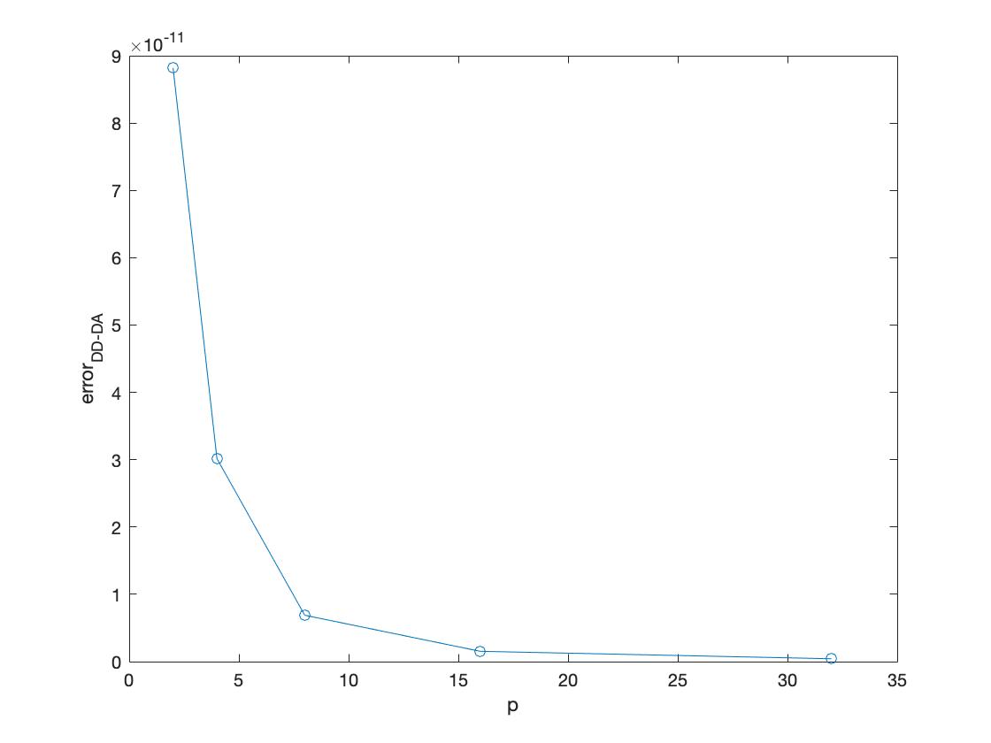
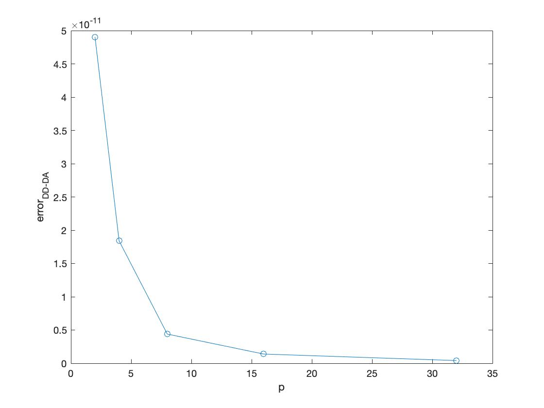
Figure 5: Examples 3 (left)- 4 (right). We report values of $error_{DD-DA}$ versus $p$.

7 Conclusions

For effective domain decomposition based parallelization, the partitioning into sub domains must satisfy certain conditions. Firstly the computational load assigned to sub domains must be equally distributed. Usually the computational cost is proportional to the amount of data entities assigned to partitions. Good quality partitioning also requires the volume of communication during calculation to be kept at its minimum. In the present work we employed a dynamic load balancing scheme based on an adaptive and dynamic redefining of initial DD aimed to balance load between processors according to data location. We call it DyDD. A mechanism for dynamically balancing the loads encountered in particular DD configurations has been included in the parallel DD framework we implement for solving large scale DA models. In particular, we focused on the introduction of a dynamic redefining of initial DD in order to deal with problems where the observations are non uniformly distributed and general sparse. This is a quite common issue in Data Assimilation. We presented first results obtained by applying DyDD in space of CLS problems using different scenarios of the initial DD. Performance results confirm the effectiveness of the algorithm. We observed that the impact of data communications required by the workload re-partitioning among sub domains affects the performance of the whole algorithm depending on the problem size and the number of available computing elements. As expected, we recognized a sort of trade off between the overhead due to the workload re-partitioning and the subsequent parallel computation. As in the assimilation window the number and the distribution of observations change, the difficulty to overcome is to implement a load balancing algorithm, which should have to dynamically allow each subdomain to move independently with time i.e. to balance observations with neighbouring subdomains, at each instant time. We are working on extending DyDD framework to such configurations.

Table 13: Procedure DyDD

Procedure DyDD-Dynamic Load Balancing(in: $p$, $\Omega$, out: $l_{1}$,…,$l_{p}$)

%Procedure DyDD allows to balance observations between adjacent subdomains

% Domain $\Omega$ is decomposed in $p$ subdomains and some of them may be empty.

% DBL procedure is composed by: DD step, Scheduling step and Migration Step.

% DD step partitions $\Omega$ in subdomains and if some subdomains have not any observations, partitions adjacent subdomains with maximum load

%in 2 subdomains and redefines the subdomains.

% Scheduling step computes the amount of observations needed for shifting boundaries of neighbouring subdomains

%Migration step decides which sub domains should be reconfigured to achieve a balanced load.

% Finally, the Update step redefines the DD.

DD step

% DD step partitions $\Omega$ in $(\Omega_{1},\Omega_{2},\ldots,\Omega_{p})$

Define $n_{i}$, the number of adjacent subdomains of $\Omega_{i}$

Define $l_{i}$: the amount of observations in $\Omega_{i}$

repeat

% identification of $\Omega_{m}$, the adjacent subdomain of $\Omega_{i}$ with the maximum load

Compute $l_{m}=max_{j=1,\ldots,n_{i}}\ (l_{j})$: the maximum amount of observations

Decompose $\Omega_{m}$ in 2 subdomains: $\Omega_{m}\leftarrow(\Omega_{m}^{1},\Omega_{m}^{2})$

until ($l_{i}\neq 0$)

end of DD Step

Begin Scheduling step

Define $G$: the graph associated with initial partition: vertex $i$ corresponds to $\Omega_{i}$

Distribute the amount of observations $l_{i}$ on $\Omega_{i}$

Define $deg(i)=n_{i}$, the degree of node $i$ of $G$:

repeat

Compute the average load: $\bar{l}=\frac{\sum_{i=1}^{p}l_{i}}{p}$

Compute load imbalance: $b={(l_{i}-\bar{l})_{i=1,\ldots,p}}$

Compute $L$, Laplacian matrix of $G$

Call solve(in:$L,b$, out:$\lambda_{i}$) % algorithm solving the linear system $L\lambda_{i}=b$

Compute $\delta_{i,j}$, the load increment between the adjacent subdomains $\Omega_{i}$ and $\Omega_{j}$. $\delta_{i,j}$ is the nearest integer of $(\lambda_{i}-\lambda_{j})$

Define $n_{s_{i}},n_{r_{i}}$, number of those subdomains whose configuration has to be updated

Update graph $G$

Update amount of observations of $\Omega_{i}$: $l_{i}=l_{i}-\sum_{j=1}^{n_{s_{i}}}\delta_{i,j}+\sum_{j=1}^{n_{r_{i}}}\delta_{j,i}$

until $(max\|l_{i}-\bar{l}\|==\frac{deg(i)}{2})$ % i.e. maximum load-difference is $deg(i)/2$

end Scheduling step

Begin Migration Step

Shift boundaries of two adjacent sub domains in order to achieve a balanced load.

end Migration Step

Update DD of $\Omega$

end Procedure DyDD

Luisa D’Amore Luisa D’Amore has the degree in Mathematics, and the Ph.D. in Applied Mathematics and Computer Science. She is professor of Numerical Analysis at University of Naples Federico II. She is member of the Academic Board of the Ph.D. in Mathematics and Applications, at University of Naples Federico II where she teaches courses of Numerical Analysis, Scientific Computing and Parallel Computing. Research activity is placed in the context of Scientific Computing. Her main interest is devoted to designing effective numerical algorithms solving ill-posed inverse problems arising in the applications, such as image analysis, medical imaging, astronomy, digital restoration of films and data assimilation. The need of computing the numerical solution within a suitable time, requires the use of advanced computing architectures. This involves designing and development of parallel algorithms and software capable of exploiting the high performance of emerging computing infrastructures. Research produces a total of about 200 publications in refereed journals and conference proceedings.

Rosalba Cacciapuoti Rosalba Cacciapuoti received the degree in Mathematics at University of Naples Federico II. She is a student of the PhD course in Mathematics and Applications at the University of Naples, Federico II. Her research activity is focused on designing of parallel algorithms for solving Data Assimilation problems.

References

- 1 L. Antonelli, L. Carracciuolo, M. Ceccarelli, L. D’Amore, A. Murli - Total Variation Regularization for Edge Preserving 3D SPECT Imaging in High Performance Computing Environments, Sloot P.M.A., Hoekstra A.G., Tan C.J.K., Dongarra J.J. (eds) Computational Science, ICCS 2002. ICCS 2002. Lecture Notes in Computer Science, vol 2330. Springer, Berlin, Heidelberg
- 2 R. Arcucci, L. D’Amore, J. Pistoia, R. Toumi, A.Murli, On the variational data assimilation problem solving and sensitivity analysis, Journal of Computational Physics, 335, pp.311-326, 2017.
- 3 Arcucci, R., D’Amore, L., Carracciuolo, L., Scotti, G., Laccetti, G. (2017). A Decomposition of the Tikhonov Regularization Functional oriented to exploit hybrid multilevel parallelism. INTERNATIONAL JOURNAL OF PARALLEL PROGRAMMING, vol. 45, p. 1214-1235, ISSN: 0885-7458, doi: 10.1007/s10766-016-0460-3
- 4 Arcucci, R., D’Amore, L., Carracciuolo, L., On the problem-decomposition of scalable 4D-Var Data Assimilation model, Proceedings of the 2015 International Conference on High Performance Computing and Simulation, HPCS 2015 2 September 2015, Pages 589-594, 13th International Conference on High Performance Computing and Simulation, HPCS 2015; Amsterdam; Netherlands; 20 July 2015 through 24 July 2015.
- 5 Arcucci, R., D’Amore, L., Celestino, S., Laccetti, G., Murli, A. (2016). A Scalable Numerical Algorithm for Solving Tikhonov Regularization Problems. In: Parallel Processing and Applied Mathematics. LECTURE NOTES IN COMPUTER SCIENCE, vol. 9574, p. 45-54, HEIDELBERG:SPRINGER, ISBN: 978-3-319-32152-3, ISSN: 0302-9743, doi: 10.1007/978-3-319-32152-3-5
- 6 G. Battistelli, L. Chisci, Stability of consensus extended Kalman filter for distributed state, Automatica Volume 68, June 2016, pp. 169-178
- 7 J. E. Boillat - Load balancing and Poisson equation in a graph, Concurrency: Practice and Experience, 2, 289-313, 1990.
- 8 M. M. Bronstein, J. Bruna, Y. LeCun, A. Szlam, P. Vandergheynst, Geometric deep learning: going beyond Euclidean, IEEE SIG PROC MAG, arXiv:1611.08097v2 [cs.CV], 3 May 2017
- 9 D.G. Cacuci. Sensitivity and Uncertanty Analysis , Chapman, Hall/Crc, NY, 2003
- 10 T. F. Chan, T. P. Mathew, Domain Decomposition algorithms, Acta Numerica, 1994, pp. 61-143.
- 11 G. Cybenco - Dynamic load balancing for distributed memory multiprocessors, Journal of Parallel and Distributed Computing, 7, 279-301, 1989.
- 12 S. E. Cohn, An introduction to estimation theory, J. Meteor. Soc. Japan, 75 (1B) (1997), pp. 257-288.
- 13 S. Cuomo, G. Severino, A. Sommella, G. D’Urso, Numerical Effects of the Gaussian Recursive Filters in Solving Linear Systems in the 3Dvar Case Study, Water Resources Research, 53 (10), pp. 8614-8625. DOI: 10.1002/2017WR020904, 2017.
- 14 L. D’Amore, R. Cacciapuoti, Model Reduction in Space and Time for decomposing ab initio 4D Variational Data Assimilation Problems, Applied Numerical Mathematics, 2021, Volume 160, pp. 242-264 Elsevier, https://doi.org/10.1016/j.apnum.2020.10.003.
- 15 D’Amore, L., Cacciapuoti, R., V. Mele - Ab initio Domain Decomposition Approaches for Large Scale Kalman Filter Methods: a case study to Constrained Least Square Problems, 13th International Conference, PPAM 2019, Bialystok, Poland, September 8-11, 2019, 10.1007/978-3-030-43222-5, LNCS Vol. 12044, Springer.
- 16 P. Diniz, S. Plimpton, B. Hendrickson, and R. Leland, Parallel algorithms for dynamically partitioning unstructured grids, in Proc. 7th SIAM Conf. Parallel Processing for Scientific Computing, SIAM, 1995, pp. 615-620.
- 17 G. Horton - A multi-level diffusion method for dynamic load balancing. Parallel Computing, 9, 209-218, 1993.
- 18 Y.F. Hu, R.J. Blake and D.R. Emerson - An optimal migration algorithm for dynamic load balancing, Concurrency: Practice and Experience 10(6):467-483, 1998.
- 19 G.A. Kohring - Dynamic load balancing for parallelized particle simulations on MIMD computers, Parallel Computing 21 pp.683-693, Elsevier, 1998.
- 20 D’Amore, L., Cacciapuoti, R., A note on domain decomposition approaches for solving 3D variational data assimilation models, Ricerche di Matematica, 2019.doi:10.1007/s11587-019-00432-4
- 21 D’Amore, L., Arcucci, R., Carracciuolo, L., Murli, A. (2014). A scalable approach for Variational Data Assimilation. JOURNAL OF SCIENTIFIC COMPUTING, vol. 61, p. 239-257, ISSN: 0885-7474, doi: 10.1007/s10915-014-9824-2
- 22 L. D’Amore, G. Laccetti, D. Romano, G. Scotti, A. Murli - Towards a parallel component in a GPU–CUDA environment: a case study with the L-BFGS Harwell routine, International Journal of Computer Mathematics Volume 92, 2015. Issue 1, https://doi.org/10.1080/00207160.2014.899589
- 23 L. D’Amore, V. Mele, D. Romano, G. Laccetti, D. Romano, A Multilevel Algebraic Approach for Performance Analysis of Parallel Algorithms, Computing and Informatics, 38 (4), DOI:10.31577/cai20194817, 2019
- 24 G. Evensen, The ensemble Kalman filter: Theoretical formulation and practical implementation, Ocean Dynam. 53 (2003) 343-367.
- 25 M. Fujimoto, M. Kawahara, Domain Decomposition for Kalman Filter Method and Its Application to Tidal Flow at Onjuku Coast, Proceedings of 12th International Conference on Domain Decomposition Methods, 2001 Editors: Tony Chan, Takashi Kako, Hideo Kawarada, Olivier Pironneau, ISBN 4-901404-00-8.
- 26 M. J. Gander, Schwarz methods over the course of time, ETNA, 31:228-255, 2008.
- 27 W. Gander, Least squares with a quadratic constraint, Numerische Mathematik, vol. 36, pp. 291-307, 1980.
- 28 C. Homescu, L. R. Petzold, R. Seban, Error Estimation for REduced Order Models of Dynamical Systems, UCRL-TR-2011494, December 2003.
- 29 R. E. Kalman, A New Approach to Linear Filtering and Prediction Problems, Transaction of the ASME - Journal of Basic Engineering, pp. 35-45, 1960.
- 30 E. Kalnay, Atmospheric Modeling, Data Assimilation and Predictability Cambridge University Press, 2003
- 31 U. A. Khan, Distributing the Kalman Filter for Large-Scale Systems, IEEE TRANSACTIONS ON SIGNAL PROCESSING, VOL. 56, NO. 10, OCTOBER 2008
- 32 A. Murli, L. D’Amore, G. Laccetti, F. Gregoretti, G. Oliva, A multi-grained distributed implementation of the parallel Block Conjugate Gradient algorithm, Concurrency Computation Practice and Experience Volume 22, Issue 15, October 2010, Pages 2053-2072
- 33 A. Murli, L. D’Amore. Regularization of a Fourier series method for the Laplace transform inversion with real data, Inverse Problems, Vol 18(4), 2002.
- 34 N. K. Nichols, Mathematical concepts of data assimilation. In: Lahoz, W., Khattatov, B. and Menard, R. (eds.) Data assimilation: making sense of observations. Springer, pp. 13-40, 2010.
- 35 J. Nocedal, S.J. Wright - Numerical Optimization, Springer-Verlag, 1999.
- 36 D. Rozier, F. Birol, E. Cosme, P. Brasseur,J. M. Brankart, J. Verron, A Reduced-Order Kalman Filter for Data Assimilation in Physical Oceanography, SIAM REVIEW, Vol. 49, No. 3, pp. 449-465, 2007
- 37 H. W. Sorenson, Least square estimation: from Gauss to Kalman, IEEE Spectrum, Vol. 7, pp. 63-68, 1970.
- 38 H.A. Schwarz. Journal fur die reine und angewandte Mathematik, 70:105-120, 1869.
- 39 C. Z. Xu and F. C. M. Lau - Analysis of the generalizes dimension exchange method for dynamic load balancing, Journal of Parallel and Distributed Computing, 16, 385-393, 1992.
- 40 C. Z. Xu and F. C. M. Lau - The generalized dimension exchange method for load balancing in K-ary ncubes and variants, Journal of Parallel and Distributed Computing, 24, 72-85, 1995.