Hadronic vacuum polarization contribution to
the muon $g-2$ in holographic QCD

Abstract

We evaluate the leading-order hadronic vacuum polarization contribution to the anomalous magnetic moment of the muon with two light flavors in minimal hard-wall and soft-wall holographic QCD models, as well as in simple generalizations thereof, and compare with the rather precise results available from dispersive and lattice approaches. While holographic QCD cannot be expected to shed light on the existing small discrepancies between the latter, this comparison in turn provides useful information on the holographic models, which have been used to evaluate hadronic light-by-light contributions where errors in data-driven and lattice approaches are more sizable. In particular, in the hard-wall model that has recently been used to implement the Melnikov-Vainshtein short-distance constraint on hadronic light-by-light contributions, a matching of the hadronic vacuum polarization to the data-driven approach points to the same correction of parameters that has been proposed recently in order to account for next-to-leading order effects.

I Introduction

Currently there is a $4.2\sigma$ discrepancy between the Standard Model prediction for the anomalous magnetic moment of the muon $a_{\mu}=(g-2)_{\mu}/2$ as assembled in the White Paper (WP) Aoyama:2020ynm and the new experimental result, obtained by combining the BNL and the Fermilab E989 values, involving an experimental error of $41\times 10^{-11}$, which is expected to be reduced further by additional data taking and future experiments. The uncertainty in the Standard Model prediction has a similar magnitude; it is almost entirely due to hadronic contributions from hadronic vacuum polarization (HVP) and from hadronic light-by-light scattering (HLbL), which according to Aoyama:2020ynm amount to

$$a_{\mu}^{\text{HVP,WP}} = (6845\pm 40)\times 10^{-11},$$ (1)

$$a_{\mu}^{\text{HLbL,WP}} = (92\pm 19)\times 10^{-11}.$$ (2)

The data-driven computation of HVP thus claims an accuracy of 0.6%, whereas the much smaller HLbL contribution has about 20% uncertainty. To match the experimental progress, improvements in the theoretical predictions for both contributions are called for.

However, the data-driven HVP result has recently been questioned by a direct lattice QCD calculation Borsanyi:2020mff by the BMW collaboration which claims a similar error of $0.8\%$

$$a_{\mu}^{\text{HVP,BMW}}=(7075\pm 55)\times 10^{-11}$$ (3)

but deviating from (1) by about 3% or $2.1\sigma$. Taken at face value this would reduce the discrepancy between experiment and theory in the case of $a_{\mu}$ to about $1.5\sigma$, while it may give rise to tensions with electroweak precision fits of the hadronic contribution to the running of the electromagnetic coupling Passera:2008jk ; Crivellin:2020zul ; Keshavarzi:2020bfy .

Once this critical issue has been resolved, it will also be crucial to reduce the theoretical uncertainty in the HLbL contribution. In the latter, an important question has been the implementation of certain short-distance constraints in hadronic models Melnikov:2003xd ; Ludtke:2020moa ; Colangelo:2021nkr , where recently holographic QCD has helped to shed light on the role of axial-vector mesons Leutgeb:2019gbz ; Cappiello:2019hwh ; Leutgeb:2021mpu ; Leutgeb:2021bpo . Holographic QCD also makes interesting quantitative predictions given the large spread of results in other hadronic models, which have led to a 100% uncertainty for the estimated contribution of axial-vector mesons in the WP. Being an approach which is based on the large color number $N_{c}$ limit, it cannot be expected to help with the percent-level discrepancies in the highly constrained HVP contribution. However, given that it typically achieves an accuracy of 10-20%, it can provide potentially useful information in the case of HLbL. Investigating the performance in the case of HVP allows us to test the holographic QCD models with regard to their ability to describe photon-hadron interactions quantitatively.

In this paper we evaluate the leading-order HVP (LO-HVP) contribution of the minimal bottom-up holographic QCD models that have been employed in the study of the HLbL contribution, as well as simple generalizations thereof, and compare with relevant results obtained within the data-driven approach, in particular for the contributions of the lightest quark flavors, revisiting and extending the study of Hong, Kim, and Matsuzaki Hong:2009jv .

As shown in Blum:2002ii ; Aubin:2006xv , the leading order HVP contributions to the muon $g-2$ is related to the hadronic vacuum polarization function through

$$a_{\mu}^{\text{LO-HVP}}=4\pi^{2}\left(\frac{\alpha}{\pi}\right)^{2}\int_{0}^{\infty}dQ^{2}f(Q^{2})\Pi_{\text{em}}^{\mathrm{had}}(Q^{2}),$$ (4)

where $Q^{2}=-q^{2}$ is the Euclidean momentum squared and

$$f(Q^{2})=\frac{m^{2}_{\mu}Q^{2}Z^{3}\left(1-Q^{2}Z\right)}{1+m^{2}_{\mu}Q^{2}Z^{2}},\quad Z=-\frac{Q^{2}-\sqrt{Q^{4}+4m^{2}_{\mu}Q^{2}}}{2m^{2}_{\mu}Q^{2}}.$$ (5)

The hadronic vacuum polarization function needs to be renormalized such that $\Pi_{\text{em}}^{\mathrm{had}}(0)=0$. It is given by the vector-current correlator, defined by

$$i\int d^{4}xe^{iqx}\langle 0|T\{J_{V}^{a\mu}(x)J_{V}^{b\nu}(0)\}|0\rangle=\delta^{ab}\left(q^{2}\eta^{\mu\nu}-q^{\mu}q^{\nu}\right)\Pi_{V}\left(-q^{2}\right)$$ (6)

in the flavor-symmetric case, via

$$\Pi_{\text{em}}^{\mathrm{had}}\left(-q^{2}\right)=2\operatorname{Tr}Q_{\text{em}}^{2}\Pi_{V}\left(-q^{2}\right),$$ (7)

where $Q_{\text{em}}=\operatorname{diag}(\frac{2}{3},-\frac{1}{3},\ldots)$ is the quark charge matrix.

As we shall show, the holographic results can deviate by up to 50% from the data-driven result, even after accounting for the fact that the holographic QCD results, being essentially a large-$N_{c}$ approximation, can only account for a subset of multi-hadron intermediate states. However, the simplest HW model that can simultaneously fit the rho meson mass and the pion decay constant as well as the leading-order short-distance behavior of the vector correlator is performing quite reasonably. Interestingly, the amount of correction expected from next-to-leading order effects in the large-momentum domain, where perturbative corrections to the asymptotic behavior proportional to $\alpha_{s}/\pi$ should play a role, turn out to be consistent with the corrections proposed recently by two of us in the case of the HLbL contribution Leutgeb:2021mpu .

In the next section, we shall review the minimal holographic QCD models included in our study to the extent necessary for evaluating the LO-HVP contribution to $a_{\mu}$ in Sect. III. Sect. IV summarizes our conclusions.

II Minimal holographic QCD models

In this work we shall limit ourselves to holographic QCD models with a minimal set of adjustable parameters with anti-de Sitter background geometry and simple generalizations thereof.

II.1 Hard-wall models

In hard-wall (HW) AdS/QCD models, a five-dimensional anti-de Sitter (AdS) background geometry is chosen. In terms of a holographic radial coordinate $z$ where the conformal boundary is at $z=0$, the line element is given by (using a mostly-minus metric convention)

$$ds^{2}=g_{MN}dx^{M}dx^{N}=\frac{1}{z^{2}}\left(\eta_{\mu\nu}dx^{\mu}dx^{\nu}-dz^{2}\right),\quad 0<z\leq z_{0}.$$ (8)

Conformal invariance is broken by a hard cutoff at $z=z_{0}$, where suitable boundary conditions for bulk fields dual to the quantum operators of the four-dimensional (large-$N_{c}$) gauge theory are imposed.

The fields dual to left and right quark bilinears $\bar{\psi}\gamma^{\mu}T^{a}P_{L,R}\psi$ are five-dimensional $U(N_{f})_{L,R}$ gauge fields $A^{(L,R)}$, where chiral symmetry breaking can be implemented through spontaneous symmetry breaking by a bifundamental scalar $X$ Erlich:2005qh ; DaRold:2005mxj or through different boundary conditions Hirn:2005nr on vector and axial-vector fields, $V=\frac{1}{2}[A^{(L)}+A^{(R)}]$ and $A=\frac{1}{2}[A^{(L)}-A^{(R)}]$, or both Domenech:2010aq .

The five-dimensional action of models with a bifundamental scalar $X$ introduced first by Erlich et al. Erlich:2005qh (termed HW1 in the following) reads

$$S=\int d^{5}x\sqrt{g}\operatorname{Tr}\left\{|DX|^{2}+3|X|^{2}-\frac{1}{4g_{5}^{2}}\left(F_{L}^{2}+F_{R}^{2}\right)\right\},$$ (9)

whereas the model of Hirn and Sanz (termed HW2) has only the Yang-Mills part.

In both cases, the field equations for transverse vector fields $\partial_{\mu}V^{\mu}=0$ are given by

$$\partial_{z}\left(\frac{1}{z}\partial_{z}V_{\mu}^{a}(q,z)\right)+\frac{q^{2}}{z}V_{\mu}^{a}(q,z)=0,$$ (10)

where we have Fourier transformed with respect to the spacetime coordinates of the boundary theory. Splitting the vector field further as $V_{\mu}^{a}(q,z)=V(q,z)v^{a}_{\mu}$, the on-shell action, given by the boundary term

$$S=-\left.\frac{1}{2g_{5}^{2}}\int d^{4}x\left(\frac{1}{z}V_{\mu}^{a}\partial_{z}V^{\mu a}\right)\right|_{z=\epsilon},$$ (11)

is interpreted as generating functional for QCD flavor currents. In both HW1 and HW2 models, boundary conditions on $V$ are such that there is no contribution from $z=z_{0}$, while the conformal boundary at $z=0$ needs regularization by a finite cutoff $z=\epsilon$ when imposing $V(q,\epsilon)=1$.

Thus we find

$$\Pi_{V}\left(-q^{2}\right)=-\left.\frac{1}{g_{5}^{2}q^{2}}\frac{\partial_{z}V(q,z)}{z}\right|_{z=\epsilon}.$$ (12)

The equations of motion (10) can be solved in terms of Bessel functions. Using the boundary conditions $V(q,\epsilon)=1$ and $\left.\partial_{z}V(q,z)\right|_{z=z_{0}}=0$ yields

$$V(q,z)=\left.\frac{zJ_{1}(qz)Y_{0}\left(qz_{0}\right)-zY_{1}(qz)J_{0}\left(qz_{0}\right)}{\epsilon J_{1}(q\epsilon)Y_{0}\left(qz_{0}\right)-\epsilon Y_{1}(q\epsilon)J_{0}\left(qz_{0}\right)}\right|_{\epsilon\rightarrow 0}.$$ (13)

Plugging this result into equation (12) yields

$$\Pi_{V}\left(-q^{2}\right)=-\frac{1}{g_{5}^{2}}\frac{1}{q\epsilon}\frac{J_{0}\left(qz_{0}\right)Y_{0}(q\epsilon)-Y_{0}\left(qz_{0}\right)J_{0}(q\epsilon)}{J_{0}\left(qz_{0}\right)Y_{1}(q\epsilon)-Y_{0}\left(qz_{0}\right)J_{1}(q\epsilon)},$$ (14)

and expanding this at $\epsilon\rightarrow 0$ gives

$$\Pi_{V}\left(-q^{2}\right)=\frac{1}{g_{5}^{2}}\left[-\frac{\pi}{2}\frac{Y_{0}\left(qz_{0}\right)}{J_{0}\left(qz_{0}\right)}+\gamma-\log 2+\log q\epsilon+\mathcal{O}\left(\epsilon^{2}\right)\right],$$ (15)

where $\gamma$ is the Euler-Mascheroni constant. This expression is divergent for $\epsilon\rightarrow 0$ and has to be renormalized. Adding a counterterm

$$S_{\mathrm{c.t.}}(\mu)=\int d^{4}x\left(\frac{1}{2g_{5}^{2}}\ln\epsilon\mu\right)\operatorname{tr}\left[F_{\mu\nu}(x,\epsilon)\right]^{2}$$ (16)

to the action gives rise to an additional term

$$\Pi_{V}^{\mathrm{c.t.}}=-\frac{1}{g_{5}^{2}}\log(\mu\epsilon),$$ (17)

which cancels the divergent part of (15). The resulting renormalized vacuum polarization is

$$\Pi_{V}^{\mathrm{ren}}\left(-q^{2}\right)=\lim_{\epsilon\rightarrow 0}\left[\Pi_{V}\left(-q^{2}\right)+\Pi_{V}^{\mathrm{c.t.}}\left(-q^{2}\right)\right]=\frac{1}{g_{5}^{2}}\left[-\frac{\pi}{2}\frac{Y_{0}\left(qz_{0}\right)}{J_{0}\left(qz_{0}\right)}+\gamma+\ln\frac{q}{2\mu}\right],$$ (18)

where $\mu$ can be chosen such that $\Pi_{V}^{\mathrm{ren}}(0)=0$ holds, as required for $\alpha$ in (4) to be identified with the standard fine structure constant in the Thomson limit. For Euclidean momenta this yields

$$\Pi_{V}^{\mathrm{ren}}\left(Q^{2}\right)=\frac{1}{g_{5}^{2}}\left[\frac{K_{0}\left(Qz_{0}\right)}{I_{0}\left(Qz_{0}\right)}+\ln\frac{Qz_{0}}{2}+\gamma\right].$$ (19)

As can be seen from (18), in the time-like domain the vacuum polarization function has an infinite series of poles at $q^{2}=m_{n}^{2}$ with $m_{n}$ given determined by $J_{0}(m_{n}z_{0})=0$, corresponding to an infinite tower of (stable) vector mesons (as expected in a large-$N_{c}$ limit). The latter are described by normalizable solutions of

$$\partial_{z}\left(\frac{1}{z}\partial_{z}\psi_{n}\right)+\frac{m_{n}^{2}}{z}\psi_{n}=0,$$ (20)

with boundary conditions $\psi_{n}^{\prime}(z_{0})=0$, $\psi_{n}(0)=0$, and are explicitly given by

$$\psi_{{n}}(z)=\frac{\sqrt{2}zJ_{1}\left(m_{n}z\right)}{z_{0}J_{1}\left(m_{n}z_{0}\right)}.$$ (21)

The unrenormalized vector current correlator can then be represented as

$$\Pi_{V}(q^{2})=\sum_{n=1}^{\infty}\frac{F_{n}^{2}}{(q^{2}-m_{n}^{2})m_{n}^{2}}$$ (22)

with decay constants $F_{n}$, defined as $\langle 0|J_{V}^{a\mu}(0)|V_{n}^{b}\rangle=F_{n}\delta^{ab}\varepsilon^{\mu}$, given by

$$F_{n}=\lim_{\epsilon\rightarrow 0}\frac{1}{g_{5}}\psi_{n}^{\prime}(\epsilon)/\epsilon=\frac{1}{g_{5}}\frac{\sqrt{2}m_{n}}{z_{0}J_{1}(m_{n}z_{0})}.$$ (23)

II.1.1 Parameters of the HW1 model

In the chiral limit, the HW1 model has only three free parameters, $g_{5}$, $z_{0}$, and the chiral condensate described by $X(z_{0})$. In the application to HLbL contributions Leutgeb:2019gbz , those were matched to the pion decay constant $f_{\pi}$, the $\rho$ meson mass, and $g_{5}$ was set such that the short-distance constraint on $\Pi_{V}$ from QCD Shifman:1978bx ; Reinders:1984sr

$$\Pi_{V}\left(Q^{2}\right)=\frac{N_{c}}{24\pi^{2}}\left(1+\frac{\alpha_{s}}{\pi}\right)\log\left(\frac{Q^{2}}{\mu^{2}}\right)-\frac{\alpha_{s}}{24\pi}\frac{N_{c}}{3}\frac{\left\langle G^{2}\right\rangle}{Q^{4}}+\frac{14N_{c}}{27}\frac{\pi\alpha_{s}\langle q\bar{q}\rangle^{2}}{Q^{6}}$$ (24)

is satisfied to leading order. This determines

$$\frac{1}{g_{5}^{2}}=\frac{N_{c}}{12\pi^{2}},$$ (25)

which holds true in other bottom-up models with bulk geometry that is at least asymptotically AdS.

The HW cutoff $z_{0}$ directly determines the mass of the lightest vector meson, which we choose as $m_{\rho}=775$ MeV, corresponding to

$$z_{0}=3.103\>\mathrm{GeV}^{-1}.$$ (26)

This remains unchanged when finite quark masses are introduced in the HW1 model; the latter modify, however, axial-vector meson masses and vector meson masses with open flavor quantum numbers Abidin:2009aj .

II.1.2 Parameters in the HW2 model

In the inherently chiral HW2 model due to Hirn and Sanz Hirn:2005nr , chiral symmetry breaking is implemented without a symmetry breaking bifundamental scalar $X$, through different boundary conditions for vector and axial-vector fields.

When $g_{5}$ and $z_{0}$ are chosen as above, the pion decay constant can no longer be fitted to phenomenological values. In the application to HLbL contributions for the muon anomalous magnetic moment Cappiello:2010uy ; Leutgeb:2019zpq ; Leutgeb:2019gbz ; Cappiello:2019hwh , which are dominated by the coupling of pions to two photons, $f_{\pi}$ is fixed first, leaving the choice of matching either the infrared parameter $m_{\rho}$ through $z_{0}$ or the ultraviolet behavior through $g_{5}$. In Leutgeb:2019zpq ; Leutgeb:2019gbz , the former option, with physical values for $f_{\pi}$ and $m_{\rho}$, is referred to as HW2 model. This matches the short-distance constraints on transition form factors and also the Melnikov-Vainshtein short-distant constraint Melnikov:2003xd only at the level of 61%. Conversely, the leading term in (24) is too large at the level of 164%. Matching these constraints at the expense of a much too heavy rho meson (987 MeV) was called HW2(UV-fit).

The symmetry breaking boundary conditions can in fact also be used in conjunction with the symmetry breaking scalar $X$. This possibility has been proposed in Domenech:2010aq and also explored in Leutgeb:2021mpu for HLbL contributions to $a_{\mu}$, where it was referred to as HW3. In the vector sector, however, this coincides with the HW1 model so that our HVP results for the latter also pertain to the HW3 case.

Summarizing the values of the parameters for the three different fits we have, for $N_{c}=3$,

$$\text{ HW1 }: \quad g_{5}=2\pi,\quad z_{0}=3.103\>\mathrm{GeV}^{-1};$$ (27)

$$\text{ HW2 }: \quad g_{5}=4.932,\quad z_{0}=3.103\>\mathrm{GeV}^{-1};$$

$$\text{ HW2 (UV-fit)}: \quad g_{5}=2\pi,\quad z_{0}=2.4359\>\mathrm{GeV}^{-1}.$$

II.2 Soft-wall model (SW)

A shortcoming of the HW models is that the masses of highly excited vector mesons do not rise as $m_{n}^{2}\sim\sigma n$ as expected from linear confinement with string constant $\sigma$, but instead like $m_{n}^{2}\sim n^{2}$.

The so-called soft-wall model introduced in Karch:2006pv (a precursor of which appeared in Ghoroku:2005vt ) achieves a strictly linear dependence of $m_{n}^{2}$ on $n$ by introducing a dilaton $\Phi(z)=\kappa^{2}z^{2}$ as an additional background field in the five-dimensional Lagrangian Karch:2006pv ; Kwee:2007dd

$$S=\int d^{5}xe^{-\Phi(z)}\sqrt{g}\operatorname{Tr}\left\{|DX|^{2}+3|X|^{2}-\frac{1}{2g_{5}^{2}}\left(F_{L}^{2}+F_{R}^{2}\right)\right\},$$ (28)

while keeping the AdS metric (8). The $z$-coordinate is, however, now unbounded from above, $z\in[0,\infty)$.

Solving the correspondingly modified field equation

$$\partial_{z}\left(\frac{e^{-\Phi}}{z}\partial_{z}V_{\mu}^{a}\right)+\frac{q^{2}e^{-\Phi}}{z}V_{\mu}^{a}=0$$ (29)

with the boundary conditions $V(q,\epsilon)=1$ in the limit $\epsilon\rightarrow 0$ and $\lim_{z\rightarrow\infty}V(q,z)=0$ gives Grigoryan:2007my

$$V(q,z)=\Gamma\left(1-\frac{q^{2}}{4\kappa^{2}}\right)U\left(\frac{-q^{2}}{4\kappa^{2}},0,(\kappa z)^{2}\right),$$ (30)

with the confluent hypergeometric function of second kind $U$ (also known as Tricomi function). Plugging this into

$$\Pi_{\mathrm{V}}\left(-q^{2}\right)=-\left.\frac{e^{-\Phi}}{g_{5}^{2}}\frac{\partial_{z}V(q,z)}{q^{2}z}\right|_{z=\epsilon}=-\left.\frac{1}{g_{5}^{2}}\frac{\partial_{z}V(q,z)}{q^{2}z}\right|_{z=\epsilon},$$ (31)

switching to the Euclidean momentum $Q^{2}=-q^{2}$ and expanding in a series for small $\epsilon$ gives

$$\Pi_{V}\left(Q^{2}\right)=\frac{1}{2g_{5}^{2}}\left[\psi\left(\frac{Q^{2}}{4\kappa^{2}}+1\right)+\ln\left(\kappa^{2}\epsilon^{2}\right)+2\gamma\right]+\mathcal{O}(\epsilon),$$ (32)

where $\psi(z)=d\ln\Gamma(z)/dz.$ Renormalizing as above and using $\psi(0)=-\gamma$ we find

$$\Pi^{\mathrm{ren}}(Q^{2})=\frac{1}{2g_{5}^{2}}\left[\psi\left(\frac{Q^{2}}{4\kappa^{2}}+1\right)+\gamma\right],$$ (33)

with $g_{5}$ fixed as in the HW1 model.

From the poles of the digamma function $\psi$ one can see that the spectrum of vector mesons is now given by

$$m_{n}^{2}=4\kappa^{2}n,\qquad n=1,2,3,\ldots.$$ (34)

Alternatively, the hadronic vacuum polarization can be calculated as above from the normalizable solutions given by Karch:2006pv ; Grigoryan:2007my

$$\psi_{n}(z)=\sqrt{\frac{2}{n}}\kappa^{2}z^{2}L_{n-1}^{1}(\kappa^{2}z^{2}),$$ (35)

where the $L_{n}^{1}$ are the generalized Laguerre polynomials of order one, leading to decay constants

$$F_{n}=\frac{1}{g_{5}}\psi_{n}^{\prime\prime}(0)=\frac{1}{g_{5}}\kappa^{2}\sqrt{8n}.$$ (36)

II.3 Interpolating models

The phenomenological study of pion form factors for HW and SW models in Kwee:2007dd came to the conclusion that the HW1 model generally performed better than the SW model. In Kwee:2007dd ; Kwee:2007nq , a simple interpolating model was proposed that combines features of HW and SW models, whereas in Casero:2007ae ; Iatrakis:2010zf ; Iatrakis:2010jb a more sophisticated version including a dynamical tachyon for chiral symmetry breaking was developed, which achieves a similar behavior.

II.3.1 Semi-hard wall model (SHW)

In the model proposed by Kwee and Lebed in Kwee:2007dd ; Kwee:2007nq , a semi-hard wall was set up by replacing the dilaton background of the SW model $e^{-\Phi}=e^{-\kappa^{2}z^{2}}$ with a background given by

$$e^{-\Phi(z)}=\frac{e^{\lambda^{2}z_{0}^{2}}-1}{e^{\lambda^{2}z_{0}^{2}}+e^{\lambda^{2}z^{2}}-2}.$$ (37)

The HW model is recovered by $\lambda z_{0}\to\infty$ at fixed $z_{0}$, whereas at large $z$ the dilaton behaves as $\Phi(z)\sim\lambda^{2}z^{2}$.

In Kwee:2007nq two sets of parameters were considered, involving $\lambda z_{0}=2.1$ and $1$, where the first choice was found to give a good agreement with the pion form factor $F_{\pi}(Q^{2})$ comparable to that of the HW1 model, albeit at the cost of not matching the pion decay constant very well; the second choice led to a similar prediction for $F_{\pi}(Q^{2})$ as the SW model.

In the following we shall choose the two free parameters $\lambda$ and $z_{0}$ such that in addition to the mass of the lightest rho meson this model reproduces the mass of $\rho(1450)$, which PDG20 lists as 1465$\pm 25$ MeV. This leads to

$$\lambda z_{0}=1.697,\quad z_{0}=2.9738\,\text{GeV}^{-1},$$ (38)

which is right in between the two parameter sets explored in Kwee:2007nq .

With (37) closed analytical results are no longer available and one has to resort to numerical solutions of the equations of motion for the vector modes. In contrast to the SW model, $m_{n}^{2}$ becomes a linear function of $n$ only for large $n$, where the spacing is determined by $m_{n+1}^{2}-m_{n}^{2}\sim 4\lambda^{2}n$ ($\approx 1.3\,\text{GeV}^{2}$ for our choice (38)). The decay constants are again given by $F_{n}=\psi^{\prime\prime}(0)/g_{5}$ with $g_{5}$ still determined by (25). Table 1 lists the results for the first 8 modes.

The full subtracted self energy function with $\Pi_{V}^{\text{ren}}(0)=0$ can then be calculated through

$$\Pi_{V}^{\text{ren }}\left(-q^{2}\right)=\sum_{n=1}^{m}\frac{q^{2}F_{{n}}^{2}}{\left(q^{2}-m_{{n}}^{2}\right)m_{{n}}^{4}}+\mathcal{O}\left(\frac{q^{2}}{m_{{m+1}}^{2}}\right).$$ (39)

II.3.2 Tachyon condensation model (TC)

Finally we consider a more sophisticated but still relatively simple bottom-up model, developed in Casero:2007ae ; Iatrakis:2010zf ; Iatrakis:2010jb , where chiral symmetry breaking is implemented by a brane-antibrane effective action with an open string tachyon mode as proposed by Sen Sen:2003tm . This is based on a pair of Dirac-Born-Infeld type Lagrangians augmented by a tachyon potential $V(|T|)$, which in the case of a single flavor reads

$$S=\int d^{4}xdzV(|T|)\left(\sqrt{\operatorname{det}\mathbf{A}^{(L)}}+\sqrt{\operatorname{det}\mathbf{A}^{(R)}}\right),$$ (40)

where

$$\mathbf{A}^{(L,R)}_{MN}=g_{MN}+\frac{2\pi\alpha^{\prime}}{g_{V}^{2}}F_{MN}^{(L,R)}+\pi\alpha^{\prime}\lambda\left[\left(D_{M}T\right)^{*}\left(D_{N}T\right)+\left(D_{N}T\right)^{*}\left(D_{M}T\right)\right],$$ (41)

and

$$D_{M}T=\left(\partial_{M}+iA_{M}^{(L)}-iA_{M}^{(R)}\right)T,\quad T=\tau e^{i\theta},$$ (42)

with a Gaussian potential

$$V=\mathcal{K}e^{-\frac{1}{2}\mu^{2}\tau^{2}}.$$ (43)

The background geometry is derived from a six-dimensional AdS soliton, which has been proposed by Kuperstein and Sonnenschein as a holographic model of four-dimensional Yang-Mills theory Kuperstein:2004yf . It is given by

$$ds_{5}^{2}=g_{tt}dt^{2}-g_{zz}dz^{2}-g_{xx}dx_{3}^{2}=\frac{R^{2}}{z^{2}}\left[dx_{1,3}^{2}-f_{\Lambda}^{-1}dz^{2}\right],$$ (44)

where $f_{\Lambda}=1-(z/z_{\Lambda})^{5}$.

Similarly to the case of the bifundamental scalar $X$ in the HW and SW models, the scalar $T$ mediates chiral symmetry breaking by its possible vacuum solutions. In order to match the scaling dimension of a quark bilinear, the AdS/CFT correspondence requires to set the mass of the field $\tau$ to

$$m_{\tau}^{2}R^{2}=-\frac{R^{2}\mu^{2}}{2\pi\alpha^{\prime}\lambda}=-3,$$ (45)

which leads to the differential equation for its profile $\tau(z)$

$$\tau^{\prime\prime}-\frac{4\mu^{2}zf_{\Lambda}}{3}\tau^{\prime 3}+\left(-\frac{3}{z}+\frac{f_{\Lambda}^{\prime}}{2f_{\Lambda}}\right)\tau^{\prime}+\left(\frac{3}{z^{2}f_{\Lambda}}+\mu^{2}\tau^{\prime 2}\right)\tau=0$$ (46)

and a UV asymptotic behavior parametrized by two constants $c_{1}$ and $c_{3}$

$$\tau=c_{1}z+\frac{\mu^{2}}{6}c_{1}^{3}z^{3}\log z+c_{3}z^{3}+\mathcal{O}\left(z^{5}\right).$$ (47)

Choosing the source parameter $c_{1}$ corresponding to the quark mass, the parameter $c_{3}$ is tuned such that the tachyon diverges exactly at $z=z_{\Lambda}$.

The parameter $\mu$ in the tachyon potential does not have a physical meaning as it can be absorbed in the definition of $\tau$; in the following it will be set to $\mu^{2}=\pi$. In Iatrakis:2010zf a fit of light unflavored mesons (composed of $u$ and $d$ quarks) gave

$$z_{\Lambda}^{-1}=522\mathrm{MeV},\quad\mathrm{c}_{1}=0.0125z_{\Lambda}^{-1}.$$ (48)

We will refer to this as TC (fit 1). In Iatrakis:2010jb the parameters are chosen as

$$z_{\Lambda}^{-1}=549\mathrm{MeV},\quad\mathrm{c}_{1}=0.0094z_{\Lambda}^{-1},$$ (49)

which gives a slightly higher mass for the lightest rho meson [referred to as TC (fit 2) in the following].

The function $\tau(z)$ we obtain as the solution of equation (46) is plotted in figure 1.

Figure 1: The tachyon field $\tau(z)$ for the parameters in (48).

The value we obtain for the other constant is

$$c_{3}\approx 0.37z_{\Lambda}^{-3}.$$ (50)

Given $\tau(z)$, one can proceed by expanding the action (40) up to quadratic order in the fields as in the other models above.

For the vector gauge fields $V_{\mu}=[A_{\mu}^{(L)}+A_{\mu}^{(R)}]/{2}$ and corresponding field strength $V_{\mu\nu}$ the action up to quadratic order reads

$$S_{V}=\frac{\left(2\pi\alpha^{\prime}\right)^{2}}{g_{V}^{4}}\mathcal{K}\int d^{4}xdze^{-\frac{1}{2}\mu^{2}\tau^{2}}\left[\frac{1}{2}\tilde{g}_{zz}^{\frac{1}{2}}V_{\mu\nu}V^{\mu\nu}+g_{xx}\tilde{g}_{zz}^{-\frac{1}{2}}\partial_{z}V_{\mu}\partial_{z}V^{\mu}\right],$$ (51)

where we have defined $\tilde{g}_{zz}=g_{zz}+2\pi\alpha^{\prime}\lambda\left(\partial_{z}\langle\tau\rangle\right)^{2}$. This leads to the mode equations

$$-\frac{1}{e^{-\frac{1}{2}\mu^{2}\tau^{2}}\tilde{g}_{zz}^{\frac{1}{2}}}\partial_{z}\left(e^{-\frac{1}{2}\mu^{2}\tau^{2}}g_{xx}\tilde{g}_{zz}^{-\frac{1}{2}}\partial_{z}\psi_{n}(z)\right)=m_{n}^{2}\psi_{n}(z).$$ (52)

As in the SHW model, solutions have to be obtained by relying on numerical calculations, which is best done by transforming the differential equations to Liouville normal form (see the Appendix of Iatrakis:2010jb ). The vector correlator, which is given by

$$\Pi_{{V}}\left(-q^{2}\right)=-\left.2\frac{\left(2\pi\alpha^{\prime}\right)^{2}\mathcal{K}R}{g_{V}^{4}}\frac{\partial_{z}V(q,z)}{q^{2}z}\right|_{z=\epsilon}.$$ (53)

for a solution with boundary condition $V(q,0)=1$, can then be calculated alternatively by summing a sufficiently large number of modes according to (39). The behavior at large $q^{2}$ can be shown Iatrakis:2010jb to be of a form similar to the SW model. Matching to the leading-order term of the OPE result leads to

$$\frac{2\left(2\pi\alpha^{\prime}\right)^{2}\mathcal{K}R}{g_{V}^{4}}=\frac{N_{c}}{12\pi^{2}}.$$ (54)

Like the SHW model, the TC model has a linear dependence of $m_{n}^{2}$ on $n$ only for large $n$, where it can be shown Iatrakis:2010jb that the spacing is given by $m_{n+1}^{2}-m_{n}^{2}\sim 6z_{\Lambda}^{-2}$ ($\approx 1.6\,\text{GeV}^{2}$ and $1.8\,\text{GeV}^{2}$ for (48) and (49), respectively).

III Numerical results

III.1 Masses and decay constants

In Table 1 we list our results for the masses and decay constants of the vector mesons in the various models. In the HW1, SW, SHW models we have fixed $m_{1}=775$ MeV while setting $g_{5}$ such that the asymptotic behavior of the vector correlator is matched. The extra parameter in the SHW model was used to additionally match $m_{2}=1465$ MeV, while in the TC model we have considered the two sets presented in Iatrakis:2010zf and Iatrakis:2010jb . The simpler HW2 model, which instead has fewer parameters, is considered in the two versions used in Leutgeb:2019gbz ; Cappiello:2019hwh for evaluating the HLbL contribution to the muon $g-2$: an IR fit where $m_{\rho}$ and $f_{\pi}$ is matched but short-distance constraints are only satisfied at the level of 61%, and a UV-fit where $f_{\pi}$ and the short-distance behavior are correct but $m_{\rho}$ too heavy by 27%.

In the HW models, the masses of excited rho mesons rise very quickly, asymptotically like $m_{n}^{2}\sim n^{2}$, whereas the SW, SHW, and TC models have $m_{n}^{2}\sim n$ as required by linear confinement. While in the HW models the first excited rho meson has a mass significantly higher than the experimental value $m_{2}=1465$ MeV, in the simple SW this value is 25% too low, this can be remedied in the SHW by our choice for its parameters, and also by the overall fits Iatrakis:2010zf ; Iatrakis:2010jb in the TC model. In the SHW and TC models, also $m_{3}$ and $m_{4}$ are well compatible with the next states on the radial Regge trajectory, which in Masjuan:2012gc were assumed to be $\rho(1900)$ and $\rho(2150)$. In Fig. 2 we plot the increments of the masses squared for the first 12 modes in the models with an asymptotically linear behavior, which shows that the simple SW model has a much smaller value ($m_{n+1}^{2}-m_{n}^{2}\equiv m_{\rho}^{2}\approx 0.601\,\text{GeV}^{2}$) than the SHW and TC models. The latter are in fact closer to the observed slope of radial Regge trajectories, which in Masjuan:2012gc was determined as $1.38(4)\,\text{GeV}^{2}$.

Regarding decay constants, sufficient experimental information is only available for the lightest rho meson through $\Gamma(\rho^{0}\to e^{+}e^{-})=7.04(6)$ keV PDG20 , which yields Donoghue:1992dd

$$F_{\rho^{0}}^{2}=3m_{\rho}^{3}\Gamma(\rho^{0}\to e^{+}e^{-})/(4\pi\alpha^{2})=[348(1)\,\text{MeV}]^{4}.$$ (55)

The largest deviations from this result, of about 25% and 20%, respectively, are found in the SW model and in the HW2(UV-fit) case, whereas the HW1 model are merely 5% too low. Note that $F_{n}\propto g_{5}^{-2}$, which implies that one could match the experimental result by a corresponding adjustment of $g_{5}$.

	HW1		HW2(IR$|$UV-fit)		SW		SHW		TC(fit$1|2$)
${n}$	$m_{n}$	$F_{n}^{1/2}$	$m_{n}$	$F_{n}^{1/2}$	$m_{n}$	$F_{n}^{1/2}$	$m_{n}$	$F_{{n}}^{1/2}$	$m_{n}$	$F_{{n}}^{1/2}$
$1$	775	$329.1$	775$|987.2$	$371.4|419.2$	775	$260.0$	775	314.0	$765.4|803.9$	$313.2|329.0$
$2$	$1779$	$615.8$	$1779|2266$	$695.1|784.5$	$1096$	$309.2$	1465	458.5	$1382|1453$	$418.0|438.9$
$3$	$2789$	$863.3$	$2789|3553$	$974.4|1100$	$1342$	$342.2$	1903	498.7	$1806|1899$	$488.7|513.0$
$4$	$3800$	$1089$	$3800|4841$	$1229|1387$	$1550$	$367.7$	2230	540.0	$2158|2269$	$538.4|564.9$
$5$	$4812$	$1300$	$4812|6130$	$1467|1656$	$1733$	$388.8$	2511	570.7	$2466|2593$	$577.3|605.4$
$6$	$5824$	$1500$	$5824|7419$	$1693|1911$	$1898$	$406.9$	2762	597.4	$2744|2885$	$610.4|639.6$
$7$	$6836$	$1692$	$6836|8708$	$1909|2155$	$2050$	$422.9$	2991	621.4	$2999|3153$	$639.4|669.7$
$8$	$7848$	$1876$	$7848|9997$	$2118|2390$	$2192$	$437.2$	3203	642.8	$3236|3402$	$665.5|696.6$

Table 1: Vector meson masses $m_{n}$ and decay constants $F_{n}^{1/2}$ in $\mathrm{MeV}$.

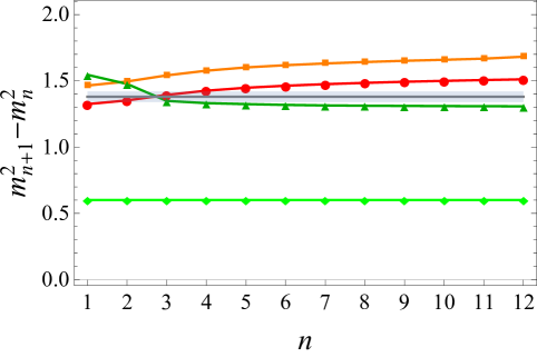
Figure 2: Plots of $m_{n+1}^{2}-m_{n}^{2}$ in GeV² in models where $m_{n}^{2}\sim n$ for large $n$: the SW model (light green), the SHW model (darker green), and the TC model (fit $1$ in red and fit $2$ in orange). The gray line is the phenomenological value given in Masjuan:2012gc as $1.38(4)\,\text{GeV}^{2}$, with the gray shaded region representing its uncertainty.

III.2 $N_{f}=2$ LO-HVP contribution to $a_{\mu}$

In Table 2 we finally give the results for the leading-order HVP contribution to the anomalous magnetic moment of the muon with two light flavors, $a_{\mu(N_{f}=2)}^{\textrm{LO-HVP}}$, by using equation (4). As mentioned above, for the HW and SW models we can use closed form expressions for $\Pi_{V}$. For the SHW and TC models we rely on numerical results and the expansion (39). The corresponding integrands in the master formula (4) are displayed in Fig. 3.

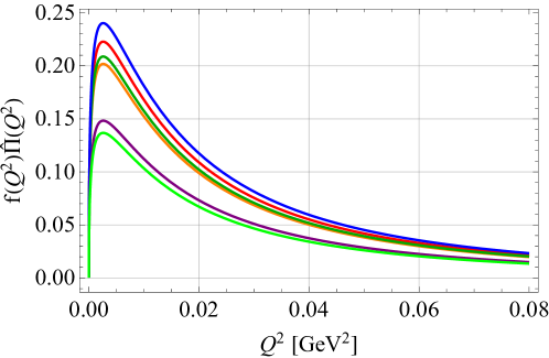
Figure 3: Plot of the integrand $f(Q^{2})\hat{\Pi}(Q^{2})=f(Q^{2})4\pi^{2}\Pi_{\text{em}}^{\mathrm{had}}(Q^{2})$ in (4) for the HW1 model (blue), SW model (light green), SHW model (darker green), and the TC model (red for fit $1$ and orange for fit $2$). The HW2 model is only shown in the version UV-fit (purple), where the UV behavior is reproduced at the expense of an unrealistically heavy rho meson; when $m_{\rho}$ and $f_{\pi}$ are fitted, the integrand peaks at about 0.39 and the UV behavior is about a factor 1.6 too large.

	$a_{\mu(N_{f}=2)}^{\text{LO-HVP}}$	mismatch
HW1	476.9	0.86
HW2(IR$|$UV-fit)	773.9$|$304.0	1.39$|$0.55
SW	$276.4$	0.50
SHW	$415.4$	0.75
TC (fit 1$|$2)	$442.3|403.6$	0.79$|$0.72

Table 2: Values of $a_{\mu}^{\text{LO-HVP}}$ with $N_{f}=2$ for the different hQCD models in multiples of $10^{-10}$. The last column gives the ratio of these results over $a_{\mu(\pi\pi,\pi\pi\pi,\pi\gamma)}^{\text{LO-HVP}}$ as obtained in the dispersive approach (56).

	DHMZ19 Davier:2019can	KNT19 Keshavarzi:2019abf
$\pi^{+}\pi^{-}$	$508(3)$	$504(2)$
$\pi^{+}\pi^{-}\pi^{0}$	$46(1)$	$47(1)$
$\pi^{0}\gamma$	4.4(1)	4.6(1)
Sum	$558(4)$	$555(3)$

Table 3: Rounded contributions of decay channels with one, two and three pions to $a_{\mu}^{\text{LO-HVP}}$ in multiples of $10^{-10}$ Aoyama:2020ynm .

With the exception of the model HW2 (with fitted $m_{\rho}$ and $f_{\pi}$), where the asymptotic behavior of $\Pi_{V}$ is about a factor 1.6 larger than the OPE result, the holographic results are much smaller than the results obtained for the $N_{f}=2$ contributions in dispersive and lattice approaches (the latter are about Aoyama:2020ynm $590\times 10^{-10}$ and Borsanyi:2020mff $640\times 10^{-10}$, respectively). However, the holographic QCD models should be viewed as (more or less crude) large-$N_{c}$ approximations. HVP contributions with multi-hadron states such as four pions correspond to higher-order contributions in the large-$N_{c}$ expansion so that it appears more reasonable to compare only with contributions from intermediate states corresponding to the $\rho$ and $\omega$ channels, which are dominated by two and three-pion states as well as $\pi^{0}\gamma$. Table 3 lists their contributions to $a_{\mu}$ according to Davier:2019can and Keshavarzi:2019abf , which combined give approximately

$$a_{\mu(\pi\pi,\pi\pi\pi,\pi\gamma)}^{\text{LO-HVP}}=557(3)\times 10^{-10}.$$ (56)

While the HW2 model in its two versions brackets this result, with rather large deviations on either side, the HW1 model, where $m_{\rho}$ and $f_{\pi}$ as well as the short-distance behavior can be fitted simultaneously, is only a factor 0.86 smaller, and thus comes closest of all models considered here.

The smallest result, at only 50%, is obtained with the SW model. As we have seen above, the SW model with a strictly linear dependence of $m_{n}^{2}$ on $n$ underestimates the masses of all excited rho mesons. While this should tend to overestimate $a_{\mu}^{\text{LO-HVP}}$, the decay constant squared of the ground-state rho meson is only at 30% of its experimental value, which is thus responsible for the strong attenuation. However, the simple modification (37) in the SHW model, which leads to a much improved mass spectrum, also brings the decay constants closer to realistic values, yielding a result for $a_{\mu}^{\text{LO-HVP}}$ that is only 25% below (56). The more sophisticated TC model turns out to be comparable, coming somewhat closer with parameters of fit 1.

Thus all models which reproduce $m_{\rho}$, $f_{\pi}$ and $F_{\rho^{0}}$ reasonably well also do not deviate too strongly from the dispersive result for $a_{\mu}^{\text{LO-HVP}}$, but uniformly underestimate it. Since the latter is proportional to $g_{5}^{-2}$, this suggests that its value, obtained from matching the leading-order term in the vector correlator (24), should be corrected to account for the next-to-leading order term, which is indeed positive. Exactly such a correction was proposed by two of us in the evaluation of the HLbL contribution within the (massive) HW1 and HW3 models Leutgeb:2021mpu ; Leutgeb:2021bpo , where it has the effect of reducing the holographic HLbL result, as this brings the asymptotic behavior of transition form factors down by amounts that are roughly consistent with perturbative corrections to the leading-order pQCD results at moderately high $Q^{2}$ values Melic:2002ij ; Bijnens:2021jqo . At the same time, the coefficient of the logarithm in the asymptotic expression (24) is increased by a similar amount, which is consistent with the next-to-leading order terms in this expression.

In the case of the HW1 model, $F_{\rho^{0}}$ can be matched by reducing $g_{5}^{2}$ by a factor $0.9$. This happens to bring the HW1 result for the $\pi^{0}$ pole contribution to the HLbL part of $a_{\mu}$ into perfect agreement with the dispersive result Leutgeb:2021mpu : $a_{\mu\text{(HW1,3)}}^{\pi^{0}}=(6.17\ldots 6.39)\times 10^{-10}$ while Hoferichter:2018kwz $a_{\mu\text{(disp.)}}^{\pi^{0}}=6.26^{+30}_{-25}\times 10^{-10}$.

With $F_{\rho^{0}}$ matched, the HW1 result for $a_{\mu}^{\text{LO-HVP}}$ becomes correspondingly larger, namely $533.2\times 10^{-10}$, which is less than 5% smaller than the dispersive result (56).

IV Conclusion

By considering a number of simple bottom-up holographic-QCD models we have found that their quantitative predictions are too spread out to be of help with the task of determining the HVP contribution to the anomalous magnetic moment of the muon, which is currently afflicted by the largest uncertainty with regard to the ongoing efforts of testing the Standard Model by a new round of experiments. However, a comparison of the holographic results for the LO-HVP contribution with the existing data-driven results at or below percent accuracy allows us to assess the various holographic models with regard to their ability to account for the relevant interactions between hadrons and photons. This is useful because holographic QCD can provide interesting estimates for HLbL contributions, where conventional approaches have uncertainties that are comparable with or larger than expected errors in the large-$N_{c}$ limit that holographic QCD is based upon.

In particular, we have considered the holographic SW and HW models that have been used previously for estimating the HLbL contributions of pseudoscalars and axial-vector mesons (see the recent review Leutgeb:2021bpo ), and we have also explored two simple extensions that aim at interpolating between the HW and SW models, while keeping their respective advantages.

We have found that the original HW1 model Erlich:2005qh turned out to come closest to the phenomenological value of the rho meson decay constant as well as to the value for $a_{\mu(N_{f}=2)}^{\text{LO-HVP}}$ obtained in dispersive approaches. The somewhat simpler HW2 model, which was used in holographic calculations of the axial-vector contribution in two versions which either fit IR or UV constraints, brackets the latter with rather large deviations in both directions. The SW model turns out to give the worst fit, but already the simple improvement of a semi-hard wall as proposed in Kwee:2007dd ; Kwee:2007nq reduces the deviation considerably; the more sophisticated TC model achieves roughly the same with the parameters considered previously in Casero:2007ae ; Iatrakis:2010zf ; Iatrakis:2010jb .

In the HW1 model, the LO-HVP result is simply proportional to the coupling $g_{5}^{-2}$ determining the asymptotic behavior of the vector correlator. Reducing $g_{5}^{2}$ by a factor 0.9 or 0.85 has been proposed in Leutgeb:2021mpu ; Leutgeb:2021bpo as a simple way to account for next-to-leading order QCD effects for the large-$Q^{2}$ behavior of transition form factors. In the case of the rho meson decay constant, a factor of 0.9 leads to a perfect fit with the phenomenological value and a result for $a_{\mu(N_{f}=2)}^{\text{LO-HVP}}$ that is only 5% too small. As shown already in Leutgeb:2021mpu ; Leutgeb:2021bpo , the same reduction of $g_{5}^{2}$ brings about a perfect agreement of the pion pole contribution in the HW1 model with the data-driven result of Hoferichter:2018kwz . We interpret this as a support for the predictions for pseudoscalar and axial-vector meson contributions obtained by two of us in various versions of the HW1 and HW3 model Leutgeb:2021mpu ; Leutgeb:2021bpo , where a theoretical error was formed by taking the unchanged results of these models as upper bound and those with $g_{5}^{2}$ reduced by a factor of 0.85 as lower bound. The corresponding values with the factor 0.9 could then be regarded as the best guess within these models.

As an outlook we would like to refer to the many possible improvements that can be considered for bottom-up holographic QCD models. In Kurachi:2013cha it has already been shown that incorporating the effects of a gluon condensate within a modified HW1 model leads to an increase of about 6% of the holographic value for $a_{\mu}^{\text{LO-HVP}}$, bringing it very close to the data-driven result. It would be interesting to study even more extensions such as models that relax the assumption $N_{f}\ll N_{c}$ of the ’t Hooft limit Jarvinen:2011qe .

- (1) T. Aoyama et al., The anomalous magnetic moment of the muon in the Standard Model, Phys. Rept. 887 (2020) 1–166, [arXiv:2006.04822].
- (2) S. Borsanyi et al., Leading hadronic contribution to the muon magnetic moment from lattice QCD, Nature 593 (2021) 51–55, [arXiv:2002.12347].
- (3) M. Passera, W. J. Marciano, and A. Sirlin, The Muon g-2 and the bounds on the Higgs boson mass, Phys. Rev. D 78 (2008) 013009, [arXiv:0804.1142].
- (4) A. Crivellin, M. Hoferichter, C. A. Manzari, and M. Montull, Hadronic Vacuum Polarization: versus Global Electroweak Fits, Phys. Rev. Lett. 125 (2020), no. 9 091801, [arXiv:2003.04886].
- (5) A. Keshavarzi, W. J. Marciano, M. Passera, and A. Sirlin, Muon and connection, Phys. Rev. D 102 (2020), no. 3 033002, [arXiv:2006.12666].
- (6) K. Melnikov and A. Vainshtein, Hadronic light-by-light scattering contribution to the muon anomalous magnetic moment revisited, Phys. Rev. D70 (2004) 113006, [hep-ph/0312226].
- (7) J. Lüdtke and M. Procura, Effects of longitudinal short-distance constraints on the hadronic light-by-light contribution to the muon , Eur. Phys. J. C 80 (2020), no. 12 1108, [arXiv:2006.00007].
- (8) G. Colangelo, F. Hagelstein, M. Hoferichter, L. Laub, and P. Stoffer, Short-distance constraints for the longitudinal component of the hadronic light-by-light amplitude: an update, Eur. Phys. J. C 81 (2021), no. 8 702, [arXiv:2106.13222].
- (9) J. Leutgeb and A. Rebhan, Axial vector transition form factors in holographic QCD and their contribution to the anomalous magnetic moment of the muon, Phys. Rev. D 101 (2020) 114015, [arXiv:1912.01596].
- (10) L. Cappiello, O. Catà, G. D’Ambrosio, D. Greynat, and A. Iyer, Axial-vector and pseudoscalar mesons in the hadronic light-by-light contribution to the muon , Phys. Rev. D 102 (2020) 016009, [arXiv:1912.02779].
- (11) J. Leutgeb and A. Rebhan, Hadronic light-by-light contribution to the muon g-2 from holographic QCD with massive pions, Phys. Rev. D 104 (2021), no. 9 094017, [arXiv:2108.12345].
- (12) J. Leutgeb, J. Mager, and A. Rebhan, Holographic QCD and the muon anomalous magnetic moment, Eur. Phys. J. C 81 (2021), no. 11 1008, [arXiv:2110.07458].
- (13) D. K. Hong, D. Kim, and S. Matsuzaki, Holographic calculation of hadronic contributions to muon g-2, Phys. Rev. D 81 (2010) 073005, [arXiv:0911.0560].
- (14) T. Blum, Lattice calculation of the lowest order hadronic contribution to the muon anomalous magnetic moment, Phys. Rev. Lett. 91 (2003) 052001, [hep-lat/0212018].
- (15) C. Aubin and T. Blum, Calculating the hadronic vacuum polarization and leading hadronic contribution to the muon anomalous magnetic moment with improved staggered quarks, Phys. Rev. D 75 (2007) 114502, [hep-lat/0608011].
- (16) J. Erlich, E. Katz, D. T. Son, and M. A. Stephanov, QCD and a holographic model of hadrons, Phys. Rev. Lett. 95 (2005) 261602, [hep-ph/0501128].
- (17) L. Da Rold and A. Pomarol, Chiral symmetry breaking from five-dimensional spaces, Nucl. Phys. B721 (2005) 79–97, [hep-ph/0501218].
- (18) J. Hirn and V. Sanz, Interpolating between low and high energy QCD via a 5-D Yang-Mills model, JHEP 12 (2005) 030, [hep-ph/0507049].
- (19) O. Domènech, G. Panico, and A. Wulzer, Massive Pions, Anomalies and Baryons in Holographic QCD, Nucl. Phys. A 853 (2011) 97–123, [arXiv:1009.0711].
- (20) M. A. Shifman, A. I. Vainshtein, and V. I. Zakharov, QCD and Resonance Physics. Theoretical Foundations, Nucl. Phys. B 147 (1979) 385–447.
- (21) L. Reinders, H. Rubinstein, and S. Yazaki, Hadron Properties from QCD Sum Rules, Phys. Rept. 127 (1985) 1.
- (22) M. Kurachi, S. Matsuzaki, and K. Yamawaki, Gluonic Effects on g-2: Holographic View, Phys. Rev. D 88 (2013) 055001, [arXiv:1306.3441].
- (23) Z. Abidin and C. E. Carlson, Strange hadrons and kaon-to-pion transition form factors from holography, Phys. Rev. D 80 (2009) 115010, [arXiv:0908.2452].
- (24) L. Cappiello, O. Cata, and G. D’Ambrosio, The hadronic light by light contribution to the with holographic models of QCD, Phys. Rev. D83 (2011) 093006, [arXiv:1009.1161].
- (25) J. Leutgeb, J. Mager, and A. Rebhan, Pseudoscalar transition form factors and the hadronic light-by-light contribution to the anomalous magnetic moment of the muon from holographic QCD, Phys. Rev. D100 (2019) 094038, [arXiv:1906.11795]. Erratum: Phys. Rev. D104, 059903 (2021).
- (26) A. Karch, E. Katz, D. T. Son, and M. A. Stephanov, Linear confinement and AdS/QCD, Phys. Rev. D74 (2006) 015005, [hep-ph/0602229].
- (27) K. Ghoroku, N. Maru, M. Tachibana, and M. Yahiro, Holographic model for hadrons in deformed AdS5 background, Phys. Lett. B 633 (2006) 602–606, [hep-ph/0510334].
- (28) H. J. Kwee and R. F. Lebed, Pion form-factors in holographic QCD, JHEP 01 (2008) 027, [arXiv:0708.4054].
- (29) H. R. Grigoryan and A. V. Radyushkin, Structure of vector mesons in holographic model with linear confinement, Phys. Rev. D76 (2007) 095007, [arXiv:0706.1543].
- (30) H. J. Kwee and R. F. Lebed, Pion Form Factor in Improved Holographic QCD Backgrounds, Phys. Rev. D 77 (2008) 115007, [arXiv:0712.1811].
- (31) R. Casero, E. Kiritsis, and A. Paredes, Chiral symmetry breaking as open string tachyon condensation, Nucl. Phys. B 787 (2007) 98–134, [hep-th/0702155].
- (32) I. Iatrakis, E. Kiritsis, and A. Paredes, An AdS/QCD model from Sen’s tachyon action, Phys. Rev. D 81 (2010) 115004, [arXiv:1003.2377].
- (33) I. Iatrakis, E. Kiritsis, and A. Paredes, An AdS/QCD model from tachyon condensation: II, JHEP 11 (2010) 123, [arXiv:1010.1364].
- (34) P. A. Zyla et al., Review of Particle Physics, Prog. Theor. Exp. Phys. 2020 (2020) 083C01. 2021 updates available on-line.
- (35) A. Sen, Dirac-Born-Infeld action on the tachyon kink and vortex, Phys. Rev. D 68 (2003) 066008, [hep-th/0303057].
- (36) S. Kuperstein and J. Sonnenschein, Non-critical, near extremal AdS6 background as a holographic laboratory of four dimensional YM theory, JHEP 11 (2004) 026, [hep-th/0411009].
- (37) P. Masjuan, E. Ruiz Arriola, and W. Broniowski, Systematics of radial and angular-momentum Regge trajectories of light non-strange -states, Phys. Rev. D 85 (2012) 094006, [arXiv:1203.4782].
- (38) J. F. Donoghue, E. Golowich, and B. R. Holstein, Dynamics of the standard model, 2nd edition. Cambridge University Press, 2014.
- (39) M. Davier, A. Hoecker, B. Malaescu, and Z. Zhang, A new evaluation of the hadronic vacuum polarisation contributions to the muon anomalous magnetic moment and to , Eur. Phys. J. C 80 (2020) 241, [arXiv:1908.00921].
- (40) A. Keshavarzi, D. Nomura, and T. Teubner, of charged leptons, , and the hyperfine splitting of muonium, Phys. Rev. D 101 (2020) 014029, [arXiv:1911.00367].
- (41) B. Melic, D. Mueller, and K. Passek-Kumericki, Next-to-next-to-leading prediction for the photon to pion transition form-factor, Phys. Rev. D68 (2003) 014013, [hep-ph/0212346].
- (42) J. Bijnens, N. Hermansson-Truedsson, L. Laub, and A. Rodríguez-Sánchez, The two-loop perturbative correction to the HLbL at short distances, JHEP 04 (2021) 240, [arXiv:2101.09169].
- (43) M. Hoferichter, B.-L. Hoid, B. Kubis, S. Leupold, and S. P. Schneider, Dispersion relation for hadronic light-by-light scattering: pion pole, JHEP 10 (2018) 141, [arXiv:1808.04823].
- (44) M. Järvinen and E. Kiritsis, Holographic Models for QCD in the Veneziano Limit, JHEP 03 (2012) 002, [arXiv:1112.1261].