Optimal Control of ensembles of dynamical systems

Abstract.

In this paper we consider the problem of the optimal control of an ensemble of affine-control systems. After proving the well-posedness of the minimization problem under examination, we establish a $\Gamma$-convergence result that allows us to substitute the original (and usually infinite) ensemble with a sequence of finite increasing-in-size sub-ensembles. The solutions of the optimal control problems involving these sub-ensembles provide approximations in the $L^{2}$-strong topology of the minimizers of the original problem. Using again a $\Gamma$-convergence argument, we manage to derive a Maximum Principle for ensemble optimal control problems with end-point cost. Moreover, in the case of finite sub-ensembles, we can address the minimization of the related cost through numerical schemes. In particular, we propose an algorithm that consists of a subspace projection of the gradient field induced on the space of admissible controls by the approximating cost functional. In addition, we consider an iterative method based on the Pontryagin Maximum Principle. Finally, we test the algorithms on an ensemble of linear systems in $\mathbb{R}^{2}$.

Keywords

Optimal control, Simultaneous control, $\Gamma$-convergence, Gradient-based minimization, Pontryagin Maximum Principle.

Mathematics Subject Classification

49J15, 49K15, 49M05.

Introduction

An ensemble of control systems is a parametrized family of controlled ODEs of the form

$$\begin{cases}\dot{x}^{\theta}(t)=G^{\theta}(x^{\theta}(t),u(t))&\mbox{a.e. in }[0,T],\\ x^{\theta}(0)=x_{0}^{\theta},\end{cases}$$ (0.1)

where $\theta\in\Theta\subset\mathbb{R}^{d}$ is the parameter of the ensemble, $u:[0,T]\to\mathbb{R}^{k}$ is the control, and, for every $\theta\in\Theta$, $G^{\theta}:\mathbb{R}^{n}\times\mathbb{R}^{k}\to\mathbb{R}^{n}$ is the function that prescribes the dynamics of the corresponding system. The peculiarity of this kind of problem is that the elements of the ensemble are simultaneously driven by the same control $u$. This framework is particularly suitable for modeling real-world control systems affected by data uncertainty (see, e.g., [28]), or the problem of controlling a large number of particles through a signal (see [9]). Also from the theoretical viewpoint, there is currently an active research interest in this topic. For instance, the problem of the controllability of ensembles of linear equations has been recently investigated in [13]. In [2] it was proved a generalization of the Chow–Rashevskii theorem for ensembles of linear-control systems. In [19, 20] ensembles were studied in the framework of nuclear magnetic resonance spectroscopy. Moreover, as regards ensembles in quantum control, we report the contributions [4, 5], and we recall the recent works [3, 11]. Finally, we mention that the interplay between Reinforced Learning and optimal control of systems affected by partially unknown dynamics has been investigated in [21, 25, 26, 24].

In the present paper, we focus on a particular instance of (0.1), corresponding to the case in which the dynamics has an affine dependence on the controls. More precisely, we consider ensembles with the following expression:

$$\begin{cases}\dot{x}^{\theta}(t)=F_{0}^{\theta}(x^{\theta}(t))+F^{\theta}(x^{\theta}(t))u(t)&\mbox{a.e. in }[0,1],\\ x^{\theta}(0)=x^{\theta}_{0},\end{cases}$$ (0.2)

where $\theta\in\Theta\subset\mathbb{R}^{d}$ varies in a compact set, and, for every $\theta\in\Theta$, the vector field $F_{0}^{\theta}:\mathbb{R}^{n}\to\mathbb{R}^{n}$ represents the drift, while the matrix-valued application $F^{\theta}=(F_{1}^{\theta},\ldots,F_{k}^{\theta}):\mathbb{R}^{n}\to\mathbb{R}^{n\times k}$ collects the controlled fields. We set $\mathcal{U}:=L^{2}([0,1],\mathbb{R}^{k})$ as the space of admissible controls, and, for every $\theta\in\Theta$, the curve $x_{u}^{\theta}:[0,1]\to\mathbb{R}^{n}$ denotes the trajectory of (0.2) corresponding to the parameter $\theta$ and to the control $u\in\mathcal{U}$. We are interested in the optimal control problem related to the minimization of a functional $\mathcal{F}:\mathcal{U}\to\mathbb{R}_{+}$ of the form

$$\mathcal{F}(u):=\int_{\Theta}\int_{0}^{1}a(t,x_{u}^{\theta}(t),\theta)\,d\nu(t)d\mu(\theta)+\frac{\beta}{2}||u||_{L^{2}}^{2}$$ (0.3)

for every $u\in\mathcal{U}$, where $a:[0,1]\times\mathbb{R}^{n}\times\Theta\to\mathbb{R}_{+}$ is a non-negative continuous function, while $\nu,\mu$ are Borel probability measures on $[0,1]$ and $\Theta$, respectively, and $\beta>0$ is a constant that tunes the $L^{2}$-squared regularization. When the support of the probability measure $\mu$ is not reduced to a finite set of points, the minimization of the functional $\mathcal{F}$ is often intractable in practical situations since a single evaluation of $\mathcal{F}$ potentially requires the resolution of an infinite number of Cauchy problems(0.2). Therefore, it is natural to try to replace $\mu$ with a sequence of probability measures $(\mu_{N})_{N\in\mathbb{N}}$ such that each of them charges a finite subset of $\Theta$, and such that $\mu_{N}\rightharpoonup^{*}\mu$ as $N\to\infty$. Then, we can consider the sequence of functionals $(\mathcal{F}^{N})_{N\in\mathbb{N}}$ defined as

$$\mathcal{F}^{N}(u):=\int_{\Theta}\int_{0}^{1}a(t,x_{u}^{\theta}(t),\theta)\,d\nu(t)d\mu_{N}(\theta)+\frac{\beta}{2}||u||_{L^{2}}^{2}$$ (0.4)

for every $u\in\mathcal{U}$ and for every $N\in\mathbb{N}$. One of the goals of the present work is to study in which sense the functionals defined in (0.4) approximate the cost $\mathcal{F}$. It turns out that, when considering the restrictions to bounded subsets of $\mathcal{U}$, the sequence $(\mathcal{F}^{N})_{N\in\mathbb{N}}$ is $\Gamma$-convergent to $\mathcal{F}$ with respect to the weak topology of $L^{2}$. We report that a similar approach was undertaken in [27], where the authors considered ensembles of control systems in the general form (0.1), and it was proved that the averaged approximations of the cost functional under examination are $\Gamma$-convergent to the original objective with respect to the strong topology of $L^{2}$. We insist on the fact that our result is not reduced to a particular case of the one studied in [27]. Indeed, on one hand, using the strong topology, in [27] it was possible to establish $\Gamma$-convergence for more general ensembles of control systems, and not only under the affine-control dynamics (0.2). On the other hand, in the general situation considered in [27] the functionals of the approximating sequence are not equi-coercive (often neither coercive) in the $L^{2}$-strong topology, and proving that the minimizers of the approximating functionals are (up to subsequences) convergent could be a challenging task. However, in the case of affine-control systems we manage to prove $\Gamma$-convergence even if the space of admissible controls $\mathcal{U}$ is equipped with the weak topology. Moreover, if for every $N\in\mathbb{N}$ we choose $u_{N}\in\arg\min_{\mathcal{U}}\mathcal{F}^{N}$, standard facts in the theory of $\Gamma$-convergence ensure that the sequence $(u_{N})_{N\in\mathbb{N}}$ is weakly pre-compact and that each of its limiting points is a minimizer of the original functional $\mathcal{F}$ defined in (0.3). What is more surprising is that –owing to the peculiar form of the cost (0.3)– it turns out that $(u_{N})_{N\in\mathbb{N}}$ is also pre-compact in the $L^{2}$-strong topology. Similar phenomena have been recently observed in [30] and [31], respectively in the frameworks of sub-Riemannian geodesics approximations and of data-driven diffeomorphisms reconstruction.

In the second part of the paper, we restrict our focus to the case of the average end-point cost, i.e., when $\nu=\delta_{t=1}$ in the integral at the right-hand side of (0.3) and (0.4). In this framework, from a direct application of the classical theory, we first derive the Pontryagin Maximum Principle for the problem of minimizing the functional $\mathcal{F}^{N}$ for $N\in\mathbb{N}$. Then, using again an argument based on the $\Gamma$-convergence, we manage to formulate the Pontryagin necessary conditions for local minimizers of the functional $\mathcal{F}$. We report that our analysis has been inspired by the results in [6], where the authors establish the Maximum Principle for a large class of ensemble optimal control problems with average end-point cost. Even though our strategy is analogous to the path described in [6] (i.e., first considering auxiliary problems involving discrete measures, and then recovering the Maximum Principle for the ensemble optimal control problem), our case is not covered by the results presented in [6]. Namely, in [6] it is required that, for every point in a neighborhood of an optimal trajectory, the set of the admissible velocities is bounded, and this fact is crucial to prove the continuity of the trajectories when the controls are equipped with the Ekeland metric (see [6, Lemma 5.1]). Moreover, we observe that in [6] the limiting process evokes Ekeland’s variational principle, while we employ $\Gamma$-convergence. Finally, we recall that in [33] the Maximum Principle for minimax optimal control was derived.

In the last part, we propose two numerical schemes for finite-ensemble optimal control problems with average end-point cost. More precisely, recalling that $\mathcal{U}$ is endowed with the usual Hilbert space structure, we first consider the gradient field induced by the functional $\mathcal{F}^{N}:\mathcal{U}\to\mathbb{R}_{+}$ on its domain. This is done by adapting to the affine-control case a result obtained in [30] for linear-control systems. Then, we construct Algorithm 1 as the orthogonal projection of this gradient field onto a subspace $\mathcal{U}_{M}\subset\mathcal{U}$ such that $\dim(\mathcal{U}_{M})<\infty$. On the other hand, Algorithm 2 is an adaptation to our problem of an iterative scheme originally proposed in [29], based on the Maximum Principle. Variants of Algorithm 1 and Algorithm 2 have been recently introduced in[31] as training procedures of a control-theoretic inspired Deep Learning architecture. We recall that a multi-shooting technique for ensemble optimal control has been recently investigated in [18].

We briefly outline the structure of this work.
In Section 1 we establish some preliminary results. In particular, we show that the trajectories of the ensemble (0.2) are uniformly $C^{0}$-stable for $L^{2}$-weakly convergent sequences of admissible controls. This property is peculiar to affine-control dynamics and plays a crucial role in the other sections.
In Section 2 we formulate the ensemble optimal control problem related to the minimization of the functional $\mathcal{F}:\mathcal{U}\to\mathbb{R}_{+}$ defined in (0.3), and we prove the existence of a solution using the direct method of calculus of variations.
In Section 3 we establish the approximation results by showing that the sequence of functionals $(\mathcal{F}^{N})_{N\in\mathbb{N}}$ defined as in (0.4) are $\Gamma$-convergent to $\mathcal{F}$ with respect to the weak topology of $L^{2}$.
In Section 4, for every $N\in\mathbb{N}$, we compute the gradient field induced by the functional $\mathcal{F}^{N}$ on the space of admissible controls, and we derive the Pontryagin Maximum Principle for the optimal control problem related to the minimization of $\mathcal{F}^{N}$. Starting from Section 4 we restrict our attention to the end-point integral cost, that corresponds to the choice $\nu=\delta_{t=1}$ in (0.3).
In Section 5 we prove the Maximum Principle for local minimizers of the functional $\mathcal{F}$, using a strategy based on $\Gamma$-convergence and the construction of auxiliary problems involving finite ensembles of control systems.
In Section 6 we construct two numerical schemes for the minimization of $\mathcal{F}^{N}$ in the case of end-point cost. The first method is based on the gradient field derived in Section 4, while for the second we make use of the Maximum Principle for finite ensembles.
Finally, in Section 7 we test the algorithms on an approximately controllable ensemble of systems in $\mathbb{R}^{2}$.

General Notations

We introduce below some basic notations. For every $d\geq 1$, we consider the space $\mathbb{R}^{d}$ endowed with the usual Euclidean norm $|z|_{2}:=\sqrt{\langle z,z\rangle_{\mathbb{R}^{d}}}$ for every $z\in\mathbb{R}^{d}$, induced by the scalar product

$$\langle x,y\rangle_{\mathbb{R}^{d}}:=\sum_{i=1}^{d}x_{i}y_{i}\qquad$$

for every $x=(x_{1},\ldots,x_{d}),y=(y_{1},\ldots,y_{d})\in\mathbb{R}^{d}$. We sometimes make use of the equivalent norm $|\cdot|_{1}$ defined as $|z|_{1}=\sum_{i=1}^{d}|z_{i}|$ for every $z\in\mathbb{R}^{d}$. We recall that the inequality

$$\frac{1}{\sqrt{d}}|z|_{2}\leq|z|_{1}\leq\sqrt{d}|z|_{2}$$ (0.5)

holds for every $z\in\mathbb{R}^{d}$.

1. Framework and Preliminary results

In this paper, we study ensembles of control systems in $\mathbb{R}^{n}$ with affine dependence in the control variable $u\in\mathbb{R}^{k}$. More precisely, given a compact set $\Theta$ embedded into a finite-dimensional Euclidean space, for every $\theta\in\Theta$ we are assigned an affine-control system of the form

$$\begin{cases}\dot{x}^{\theta}(t)=F_{0}^{\theta}(x^{\theta}(t))+F^{\theta}(x^{\theta}(t))u(t),\\ x^{\theta}(0)=x^{\theta}_{0},\end{cases}$$ (1.1)

where for every $\theta\in\Theta$ we require that $F_{0}^{\theta}:\mathbb{R}^{n}\to\mathbb{R}^{n}$ and $F^{\theta}:\mathbb{R}^{n}\to\mathbb{R}^{n\times k}$ are Lipschitz-continuous applications. We stress the fact that the control $u:[0,1]\to\mathbb{R}^{k}$ does not depend on $\theta$, so it is the same for every control system of the ensemble. Let us introduce $F_{0}:\mathbb{R}^{n}\times\Theta\to\mathbb{R}^{n}$ and $F:\mathbb{R}^{n}\times\Theta\to\mathbb{R}^{n\times k}$ defined respectively as

$$F_{0}(x,\theta):=F_{0}^{\theta}(x)\qquad\mbox{and}\qquad F(x,\theta):=F^{\theta}(x)$$ (1.2)

for every $(x,\theta)\in\mathbb{R}^{n}\times\Theta$. We assume that $F_{0}$ and $F$ are Lipschitz-continuous mappings, i.e., that there exists a constant $L>0$ such that

$$|F_{0}(x_{1},\theta_{1})-F_{0}(x_{2},\theta_{2})|_{2}\leq L\big{(}|x_{1}-x_{2}|_{2}+|\theta_{1}-\theta_{2}|_{2}\big{)}$$ (1.3)

and

$$\sup_{i=1,\ldots,k}|F_{i}(x_{1},\theta_{1})-F_{i}(x_{2},\theta_{2})|_{2}\leq L\big{(}|x_{1}-x_{2}|_{2}+|\theta_{1}-\theta_{2}|_{2}\big{)}$$ (1.4)

for every $(x_{1},\theta_{1}),(x_{2},\theta_{2})\in\mathbb{R}^{n}\times\Theta$. In (1.4) we used $F_{i}(x,\theta)$ to denote the vector obtained by taking the $i^{\mathrm{th}}$ column of the matrix $F(x,\theta)$, for every $i=1,\ldots,k$. Similarly, for every $\theta\in\Theta$ we shall use $F^{\theta}_{i}:\mathbb{R}^{n}\to\mathbb{R}^{n}$ to denote the vector field corresponding to the $i^{\mathrm{th}}$ column of the matrix-valued application $F^{\theta}:\mathbb{R}^{n}\to\mathbb{R}^{n\times k}$. We observe that (1.3)-(1.4) imply that the vector fields $F_{0}^{\theta},F_{1}^{\theta},\ldots,F_{k}^{\theta}$ are uniformly Lipschitz-continuous as $\theta$ varies in $\Theta$. Another consequence of the Lipschitz-continuity conditions (1.3)-(1.4) is that the vector fields constituting the affine-control system (1.1) have sub-linear growth, uniformly with respect to the dependence on $\theta$. Namely, we have that there exists a constant $C>0$ such that

$$\sup_{\theta\in\Theta}|F_{0}^{\theta}(x)|_{2}\leq C\big{(}|x|_{2}+1)$$ (1.5)

and

$$\sup_{\theta\in\Theta}\,\sup_{i=1,\ldots,k}|F^{\theta}_{i}(x)|_{2}\leq C\big{(}|x|_{2}+1)$$ (1.6)

for every $x\in\mathbb{R}^{n}$. Finally, let us consider the application $x_{0}:\Theta\to\mathbb{R}^{n}$ that prescribes the initial state of (1.1), i.e.,

$$x_{0}(\theta):=x_{0}^{\theta}$$ (1.7)

for every $\theta\in\Theta$. We assume that $x_{0}$ is continuous. As a matter of fact, there exists a constant $C^{\prime}>0$ such that

$$\sup_{\theta\in\Theta}|x_{0}(\theta)|_{2}\leq C^{\prime}.$$ (1.8)

We set $\mathcal{U}:=L^{2}([0,1],\mathbb{R}^{k})$ as the space of admissible controls, and we equip it with the usual Hilbert space structure given by the scalar product

$$\langle u,v\rangle_{L^{2}}:=\int_{0}^{1}\langle u(t),v(t)\rangle_{\mathbb{R}^{k}}\,dt$$ (1.9)

for every $u,v\in\mathcal{U}$. For every $u\in\mathcal{U}$ and $\theta\in\Theta$, the curve $x_{u}^{\theta}:[0,1]\to\mathbb{R}^{n}$ denotes the solution of the Cauchy problem (1.1) corresponding to the system identified by $\theta$ and to the admissible control $u$. We recall that, for every $u\in\mathcal{U}$ and $\theta\in\Theta$, the existence and uniqueness of the solution of (1.1) are guaranteed by the Carathéodory Theorem (see, e.g., [17, Theorem 5.3]). Given $u\in\mathcal{U}$, we describe the evolution of the ensemble of control systems (1.1) through the mapping $X_{u}:[0,1]\times\Theta\to\mathbb{R}^{n}$ defined as follows:

$$X_{u}(t,\theta):=x_{u}^{\theta}(t)$$ (1.10)

for every $(t,\theta)\in[0,1]\times\Theta$. In other words, for every $u\in\mathcal{U}$ the application $X_{u}$ collects the trajectories of the ensemble of control systems (1.1). We study the properties of the mapping $X_{u}$ in Subsection 1.2 below. Before proceeding, we recall some elementary facts in functional analysis.

1.1. General results in functional analysis

We begin by recalling some basic facts about the space of admissible controls $\mathcal{U}:=L^{2}([0,1],\mathbb{R}^{k})$. First of all, the linear inclusion $\mathcal{U}\hookrightarrow L^{1}([0,1],\mathbb{R}^{k})$ is continuous, and from (0.5) and the Jensen inequality it follows that

$$||u||_{L^{1}}:=\int_{0}^{1}|u(\tau)|_{1}\,d\tau\leq\sqrt{k}||u||_{L^{2}}$$ (1.11)

for every $u\in\mathcal{U}$. We shall often make use of $L^{2}$-weakly convergent sequences. Given a sequence $(u_{m})_{m\in\mathbb{N}}\subset\mathcal{U}$, we say that $(u_{m})_{m\in\mathbb{N}}$ is convergent to $u\in\mathcal{U}$ with respect to the weak topology of $L^{2}$ if

$$\lim_{m\to\infty}\langle v,u_{m}\rangle_{L^{2}}=\langle v,u\rangle_{L^{2}}$$

for every $v\in\mathcal{U}$, and we write $u_{m}\rightharpoonup_{L^{2}}u$ as $m\to\infty$. If $u_{m}\rightharpoonup_{L^{2}}u$ as $m\to\infty$, then we have

$$||u||_{L^{2}}\leq\liminf_{m\to\infty}||u_{m}||_{L^{2}}.$$ (1.12)

Finally, we recall that any bounded sequence $(u_{m})_{m\in\mathbb{N}}$ is pre-compact with respect to the $L^{2}$-weak topology. For further details on weak topologies of Banach spaces, the reader is referred to [8, Chapter 3]. We conclude this part with the following fact concerning the one-dimensional Sobolev space $H^{1}([a,b],\mathbb{R}^{d}):=W^{1,2}([a,b],\mathbb{R}^{d})$. For a complete survey on the topic, we recommend [8, Chapter 8].

Proposition 1.1.

Let $f:[a,b]\to\mathbb{R}^{d}$ be a function in $H^{1}([a,b],\mathbb{R}^{d})$. Then, $f$ is Hölder-continuous with exponent $\frac{1}{2}$, namely

$$|f(t_{1})-f(t_{2})|_{2}\leq||f^{\prime}||_{L^{2}}|t_{1}-t_{2}|^{\frac{1}{2}}$$

for every $t_{1},t_{2}\in[a,b]$, where $f^{\prime}\in L^{2}([0,1],\mathbb{R}^{d})$ denotes the weak derivative of $f$.

1.2. Trajectories of the controlled ensemble

We now investigate the evolution of the ensemble of control systems (1.1) when we consider a sequence of $L^{2}$-weakly convergent admissible controls. The proof is postponed to the end of the present subsection.

Proposition 1.2.

Let us consider a sequence of admissible controls $(u_{m})_{m\in\mathbb{N}}\subset\mathcal{U}$ such that $u_{m}\rightharpoonup_{L^{2}}u_{\infty}$ as $m\to\infty$. For every $m\in\mathbb{N}\cup\{\infty\}$, let $X_{m}:[0,1]\times\Theta\to\mathbb{R}^{n}$ be the application defined in (1.10) that collects the trajectories of the ensemble of control systems (1.1) corresponding to the admissible control $u_{m}$. Therefore, we have that

$$\lim_{m\to\infty}\,\sup_{(t,\theta)\in[0,1]\times\Theta}|X_{m}(t,\theta)-X_{\infty}(t,\theta)|_{2}=0.$$ (1.13)

Remark 1.

Proposition 1.2 is the cornerstone of the theoretical results presented in this paper. Indeed, the fact fact that the trajectories of the ensemble (1.1) are uniformly convergent when the corresponding controls are $L^{2}$-weakly convergent is used both to prove the existence of optimal controls (see Theorem 2.2) and to establish the $\Gamma$-convergence result (see Theorem 3.3). We stress that the fact that the systems in the ensemble (1.2) have affine dependence in the controls is crucial for the proof of Proposition 1.2.

In view of the next auxiliary result, we introduce some notations. For every $\theta\in\Theta$, we define $\tilde{F}^{\theta}:\mathbb{R}^{n}\to\mathbb{R}^{n\times(k+1)}$ as follows:

$$\tilde{F}^{\theta}(x):=(F_{0}^{\theta}(x),F^{\theta}(x)),$$ (1.14)

for every $x\in\mathbb{R}^{n}$, i.e., we add the column $F^{\theta}_{0}(x)$ to the $n\times k$ matrix $F^{\theta}(x)$. Similarly, for every $u\in\mathcal{U}=L^{2}([0,1],\mathbb{R}^{k})$, we consider the extended control $\tilde{u}\in\tilde{\mathcal{U}}:=L^{2}([0,1],\mathbb{R}^{k+1})$ defined as

$$\tilde{u}(t)=(1,u(t))^{T}$$ (1.15)

for every $t\in[0,1]$, i.e., we add the component $u_{0}=1$ to the column-vector $u(t)$.

Lemma 1.3.

Let us consider a sequence of admissible controls $(u_{m})_{m\in\mathbb{N}}\subset\mathcal{U}$ such that $u_{m}\rightharpoonup_{L^{2}}u_{\infty}$ as $m\to\infty$. For every $m\in\mathbb{N}\cup\{\infty\}$ and for every $\theta\in\Theta$, let $x_{m}^{\theta}:[0,1]\to\mathbb{R}^{n}$ be the solution of (1.1) corresponding to the ensemble parameter $\theta$ and to the admissible control $u_{m}$. Then, for every $\theta\in\Theta$ we have

$$\lim_{m\to\infty}||x_{m}^{\theta}-x_{\infty}^{\theta}||_{C^{0}}=0.$$ (1.16)

Proof.

Let us fix $\theta\in\Theta$. By means of the matrix-valued function $\tilde{F}:\mathbb{R}^{n}\to\mathbb{R}^{n\times(k+1)}$ and the extended control $\tilde{u}:[0,1]\to\mathbb{R}^{k+1}$ defined in (1.14) and (1.15) respectively, we can equivalently rewrite the affine-control system (1.1) corresponding to $\theta$ as follows:

$$\begin{cases}\dot{x}^{\theta}=\tilde{F}^{\theta}(x^{\theta})\tilde{u},\\ x^{\theta}(0)=x^{\theta}_{0},\end{cases}$$ (1.17)

for every $u\in\mathcal{U}$. In other words, any solution $x_{u}^{\theta}:[0,1]\to\mathbb{R}^{n}$ of (1.1) corresponding to the admissible control $u\in\mathcal{U}$ is in turn a solution of the linear-control system (1.17) corresponding to the extended control $\tilde{u}\in\tilde{\mathcal{U}}$. On the other hand, the convergence $u_{m}\rightharpoonup_{L^{2}}u_{\infty}$ as $m\to\infty$ implies the convergence of the respective extended controls, i.e., $\tilde{u}_{m}\rightharpoonup_{L^{2}}\tilde{u}_{\infty}$ as $m\to\infty$. Therefore, $(x_{m}^{\theta})_{m\in\mathbb{N}}$ is the sequence of solutions of the linear-control system (1.17) corresponding to the $L^{2}$-weakly convergent sequence of controls $(\tilde{u}_{m})_{m\in\mathbb{N}}$. Moreover, $x^{\theta}_{\infty}$ is the solution of (1.17) associated with the weak-limiting control $\tilde{u}_{\infty}$. Using [30, Lemma 7.1], we deduce (1.16). ∎

We are now in position to prove Proposition 1.2.

Proof of Proposition 1.2.

Let us consider a $L^{2}$-weakly convergent sequence $(u_{m})_{m\in\mathbb{N}}\subset\mathcal{U}$ such that $u_{m}\rightharpoonup_{L^{2}}u_{\infty}$ as $m\to\infty$. We immediately deduce that there exists $R>0$ such that $||u_{m}||_{L^{2}}^{2}\leq R$ for every $m\in\mathbb{N}\cup\{\infty\}$. Thus, in virtue of Lemma A.5, we deduce that the sequence of mappings $\{X_{m}:[0,1]\times\Theta\to\mathbb{R}^{n}\}_{m\in\mathbb{N}}$ is uniformly equi-continuous, while Lemma A.2 guarantees that it is uniformly equi-bounded. Therefore, applying the Ascoli-Arzelà Theorem (see, e.g., [8, Theorem 4.25]), we deduce that the family $(X_{m})_{m\in\mathbb{N}}$ is pre-compact with respect to the strong topology of the Banach space $C^{0}([0,1]\times\Theta,\mathbb{R}^{n})$. Finally, Lemma 1.3 implies that

$$\lim_{m\to\infty}X_{m}(t,\theta)=X_{\infty}(t,\theta)$$

for every $(t,\theta)\in[0,1]\times\Theta$. In particular, we deduce that the set of limiting points of the pre-compact sequence $(X_{m})_{m\in\mathbb{N}}$ is reduced to the single-element set $\{X_{\infty}\}$. This proves (1.13). ∎

1.3. Adjoint variables of the controlled ensemble

In this subsection we introduce a function $\Lambda_{u}$, which will play a crucial role in Section 5. Here we consider an assigned function $a:\mathbb{R}^{n}\times\Theta\to\mathbb{R}$ such that $(x,\theta)\mapsto\nabla_{x}a(x,\theta)$ is continuous. Moreover, we further require that $(x,\theta)\mapsto\frac{\partial}{\partial x}F_{i}(x,\theta)$ is continuous for every $i=0,\ldots,k$. For every $u\in\mathcal{U}$ and every $\theta\in\Theta$, we define the function $\lambda_{u}^{\theta}:[0,1]\to(\mathbb{R}^{n})^{*}$ as the solution of the following differential equation

$$\begin{cases}\dot{\lambda}_{u}^{\theta}(t)=-\lambda_{u}^{\theta}(t)\left(\frac{\partial F_{0}(x_{u}^{\theta}(t),\theta)}{\partial x}+\sum_{i=1}^{k}u_{i}(t)\frac{\partial F_{i}(x_{u}^{\theta}(t),\theta)}{\partial x}\right),\\ \lambda_{u}^{\theta}(1)=\nabla_{x}a(x_{u}^{\theta}(1),\theta),\end{cases}$$ (1.18)

where the curve $x_{u}^{\theta}:[0,1]\to\mathbb{R}^{n}$ is the solution of the Cauchy problem (1.1) corresponding to the system identified by $\theta$ and to the admissible control $u$. We insist on the fact that in this paper $\lambda_{u}^{\theta}$ is always understood as a row-vector, as well as any other element of $(\mathbb{R}^{n})^{*}$. The existence and the uniqueness of the solution of (1.18) follow as a standard application of the Carathéodory Theorem (see, e.g., [17, Theorem 5.3]). Similarly as done in the previous subsection, for every $u\in\mathcal{U}$ we introduce the function $\Lambda_{u}:[0,1]\times\Theta\to(\mathbb{R}^{n})^{*}$ defined as

$$\Lambda_{u}(t,\theta):=\lambda_{u}^{\theta}(t).$$ (1.19)

In the case of a sequence of weakly convergent controls $(u_{m})_{m\in\mathbb{N}}$, for the corresponding sequence $(\Lambda_{u_{m}})_{m\in\mathbb{N}}$ we can establish a result analogue to Proposition 1.2.

Proposition 1.4.

Let us assume that the mappings $(x,\theta)\mapsto\frac{\partial}{\partial x}F_{i}(x,\theta)$ are continuous for every $i=0,\ldots,k$, as well as the gradient $(x,\theta)\mapsto\nabla_{x}a(x,\theta)$. Let us consider a sequence of admissible controls $(u_{m})_{m\in\mathbb{N}}\subset\mathcal{U}$ such that $u_{m}\rightharpoonup_{L^{2}}u_{\infty}$ as $m\to\infty$. For every $m\in\mathbb{N}\cup\{\infty\}$, let $\Lambda_{m}:[0,1]\times\Theta\to(\mathbb{R}^{n})^{*}$ be the application defined in (1.19) that collects the adjoint variables (1.18) corresponding to the admissible control $u_{m}$. Then, we have that

$$\lim_{m\to\infty}\,\sup_{(t,\theta)\in[0,1]\times\Theta}|\Lambda_{m}(t,\theta)-\Lambda_{\infty}(t,\theta)|_{2}=0.$$ (1.20)

Before detailing the proof of Proposition 1.4, we establish an auxiliary result with a similar flavor as Lemma 1.3.

Lemma 1.5.

Let us assume that the mappings $(x,\theta)\mapsto\frac{\partial}{\partial x}F_{i}(x,\theta)$ are continuous for every $i=0,\ldots,k$, as well as the gradient $(x,\theta)\mapsto\nabla_{x}a(x,\theta)$. Let us consider a sequence of admissible controls $(u_{m})_{m\in\mathbb{N}}\subset\mathcal{U}$ such that $u_{m}\rightharpoonup_{L^{2}}u_{\infty}$ as $m\to\infty$. For every $m\in\mathbb{N}\cup\{\infty\}$ and for every $\theta\in\Theta$, let $\lambda_{m}^{\theta}:[0,1]\to(\mathbb{R}^{n})^{*}$ be the solution of (1.18) corresponding to the ensemble parameter $\theta$ and to the admissible control $u_{m}$. Then, for every $t\in[0,1]$ and for every $\theta\in\Theta$, we have

$$\lim_{m\to\infty}||\lambda_{m}^{\theta}(t)-\lambda_{\infty}^{\theta}(t)||_{C^{0}}=0.$$ (1.21)

Proof.

The weak convergence $u_{m}\rightharpoonup_{L^{2}}u_{\infty}$ as $m\to\infty$ implies that there exists $R>0$ such that $||u_{m}||_{L^{2}}\leq R$ for every $m\in\mathbb{N}\cup\{\infty\}$. Let us fix $\theta\in\Theta$. With the same argument as in the proof of Lemma B.2 we deduce that the sequence $(\lambda_{m}^{\theta})_{m\in\mathbb{N}}\subset H^{1}([0,1],\mathbb{R}^{k})$ is equi-bounded. Therefore, there exists a weakly convergent subsequence $(\lambda_{m_{\ell}}^{\theta})_{\ell\in\mathbb{N}}$ such that $\lambda_{m_{\ell}}^{\theta}\rightharpoonup_{H^{1}}\bar{\lambda}^{\theta}$ as $\ell\to\infty$. Moreover, this implies that $\dot{\lambda}_{m_{\ell}}^{\theta}\rightharpoonup_{L^{2}}\dot{\bar{\lambda}}^{\theta}$ as $\ell\to\infty$, while from the compact inclusion $H^{1}\hookrightarrow C^{0}$ we deduce that $\lambda_{m_{\ell}}^{\theta}\to_{C^{0}}\bar{\lambda}^{\theta}$ as $\ell\to\infty$. In particular, this last convergence and Lemma 1.3 imply that

$$\bar{\lambda}^{\theta}(1)=\lim_{\ell\to\infty}\lambda_{m_{\ell}}^{\theta}(1)=\lim_{\ell\to\infty}\nabla_{x}a(x^{\theta}_{m_{\ell}}(1),\theta)=\nabla_{x}a(x^{\theta}_{\infty}(1),\theta),$$ (1.22)

where for every $m\in\mathbb{N}\cup\{\infty\}$ the curve $x^{\theta}_{m}:[0,1]\to\mathbb{R}^{n}$ denotes the solution of (1.1) corresponding to the control $u_{m}$ and to the parameter $\theta$. We want to prove that $\bar{\lambda}^{\theta}:[0,1]\to(\mathbb{R}^{n})^{*}$ is the solution of (1.18) corresponding to the control $u_{\infty}$. We recall that

$$\dot{\lambda}_{m_{\ell}}^{\theta}=\lambda_{m_{\ell}}^{\theta}\left(\frac{\partial F_{0}(x_{m_{\ell}}^{\theta}(\cdot),\theta)}{\partial x}+\sum_{i=1}^{k}u_{i,{m_{\ell}}}\frac{\partial F_{i}(x_{m_{\ell}}^{\theta}(\cdot),\theta)}{\partial x}\right)$$ (1.23)

for every $\ell\in\mathbb{N}$. We observe that, in virtue of Lemma A.2, there exists $K_{R}\subset\mathbb{R}^{n}$ such that $x_{m}^{\theta}(t)\in K_{R}$ for every $m\in\mathbb{N}\cup\{\infty\}$ and for every $(t,\theta)\in[0,1]\times\Theta$. Then, owing to the continuity of the mappings $(x,\theta)\mapsto\frac{\partial}{\partial x}F_{i}(x,\theta)$ for every $i=0,\ldots,k$, we deduce the convergence $\frac{\partial}{\partial x}F_{i}(x_{m_{\ell}}(\cdot),\theta)\to_{C^{0}}\frac{\partial}{\partial x}F_{i}(x_{\infty}(\cdot),\theta)$ as $\ell\to\infty$ for every $i=0,\ldots,k$. Summarizing, we have that

$$\begin{cases}\dot{\lambda}_{m_{\ell}}^{\theta}\rightharpoonup_{L^{2}}\dot{\bar{\lambda}}^{\theta}\\ \lambda_{m_{\ell}}^{\theta}\to_{C^{0}}\bar{\lambda}^{\theta}\\ u_{i,m_{\ell}}\rightharpoonup_{L^{2}}u_{i,\infty}&\mbox{for every }i=1,\ldots,k,\\ \frac{\partial}{\partial x}F_{i}(x_{m_{\ell}}(\cdot),\theta)\to_{C^{0}}\frac{\partial}{\partial x}F_{i}(x_{\infty}(\cdot),\theta)&\mbox{for every }i=0,\ldots,k,\end{cases}\quad\mbox{ as }\ell\to\infty.$$ (1.24)

Combining (1.23) and (1.24), we derive that

$$\dot{\bar{\lambda}}^{\theta}=\bar{\lambda}^{\theta}\left(\frac{\partial F_{0}(x_{\infty}^{\theta}(\cdot),\theta)}{\partial x}+\sum_{i=1}^{k}u_{i,\infty}\frac{\partial F_{i}(x_{\infty}^{\theta}(\cdot),\theta)}{\partial x}\right).$$ (1.25)

The identities (1.22) and (1.25) show that $\bar{\lambda}^{\theta}\equiv\lambda_{\infty}^{\theta}$, where $\lambda_{\infty}^{\theta}:[0,1]\to(\mathbb{R}^{n})^{*}$ is the unique solution of (1.18) corresponding to the control $u_{\infty}$. Hence, since any $H^{1}$-weakly convergent subsequence of $(\lambda_{m}^{\theta})_{m\in\mathbb{N}}$ must converge to $\lambda_{\infty}^{\theta}$, we get (1.21). Since this argument holds for every choice of $\theta\in\Theta$, we deduce the thesis. ∎

We are now able to prove Proposition 1.4.

Proof of Proposition 1.4.

The argument is the same as in the proof of Proposition 1.2. Namely, Lemma 1.5 guarantees the pointwise convergence of the mappings $(\Lambda_{m})_{m\in\mathbb{N}}$ to $\Lambda_{\infty}$, while Lemma B.1 and Lemma B.4 ensure, respectively, that the elements of the sequence are uniformly equi-bounded and uniformly equi-continuous. ∎

1.4. Gradient field for affine-control systems with end-point cost

In this subsection we generalize to the case of affine-control systems some of the results obtained in [30] in the framework of linear-control systems with end-point cost. As we shall see, the strategy that we pursue consists in embedding the affine-control system into a larger linear-control system, similarly as done in the proof of Lemma 1.3. Therefore, we can exploit a consistent part of the machinery developed in [30] to cover the present case. Let us consider a single affine-control system on $\mathbb{R}^{n}$ of the form

$$\begin{cases}\dot{x}(t)=F_{0}(x(t))+F(x(t))u(t),&\mbox{for a.e. }t\in[0,1],\\ x(0)=x_{0},\end{cases}$$ (1.26)

where $F_{0}:\mathbb{R}^{n}\to\mathbb{R}^{n}$ and $F:\mathbb{R}^{n}\to\mathbb{R}^{n\times k}$ are $C^{2}$-regular applications that design the affine-control system, and $u\in\mathcal{U}=L^{2}([0,1],\mathbb{R}^{k})$ is the control. We introduce the functional $\mathcal{J}:\mathcal{U}\to\mathbb{R}$ defined on the space of admissible controls as follows:

$$\mathcal{J}(u):=a(x_{u}(1))+\frac{\beta}{2}||u||_{L^{2}}^{2}$$ (1.27)

for every $u\in\mathcal{U}$, where $a:\mathbb{R}^{n}\to\mathbb{R}$ is a $C^{2}$-regular function and $\beta>0$ a positive parameter. After proving that the functional $\mathcal{J}$ is differentiable, we provide the Riesz’s representation of the differential $d_{u}\mathcal{J}:\mathcal{U}\to\mathbb{R}$.

Before proceeding, it is convenient to introduce the linear-control system in which we embed (1.26). Similar to (1.14), let $\tilde{F}:\mathbb{R}^{n}\to\mathbb{R}^{n\times(k+1)}$ be the function defined as

$$\tilde{F}(x):=(F_{0}(x),F(x))$$ (1.28)

for every $x\in\mathbb{R}^{n}$. If we define the extended space of admissible controls as $\tilde{\mathcal{U}}:=L^{2}([0,1],\mathbb{R}^{k+1})$, we may consider the following linear-control system

$$\begin{cases}\dot{x}(t)=\tilde{F}(x(t))\tilde{u}(t)&\mbox{for a.e. }t\in[0,1],\\ x(0)=x_{0},\end{cases}$$ (1.29)

where $\tilde{u}\in\tilde{\mathcal{U}}$. We observe that we can recover the affine system (1.26) by restricting the set of admissible controls in (1.29) to the image of the affine embedding $i:\mathcal{U}\to\tilde{\mathcal{U}}$ defined as

$$i[u]:=\left(\begin{matrix}1\\ u\end{matrix}\right).$$ (1.30)

We introduce the extended cost functional $\tilde{\mathcal{J}}:\tilde{\mathcal{U}}\to\mathbb{R}$ as

$$\tilde{\mathcal{J}}(\tilde{u}):=a(x_{\tilde{u}}(1))+\frac{\beta}{2}||\tilde{u}||_{L^{2}}^{2}$$ (1.31)

for every $\tilde{u}\in\tilde{\mathcal{U}}$, where $x_{\tilde{u}}:[0,1]\to\mathbb{R}^{n}$ is the absolutely continuous solution of (1.29) corresponding to the control $\tilde{u}$. To avoid confusion, in the present subsection we denote by $\langle\cdot,\cdot\rangle_{\mathcal{U}}$ and $\langle\cdot,\cdot\rangle_{\tilde{\mathcal{U}}}$ the scalar products in $\mathcal{U}$ and $\tilde{\mathcal{U}}$, respectively. In the next result we prove that the functional $\mathcal{J}:\mathcal{U}\to\mathbb{R}$ defined in (1.27) is differentiable.

Proposition 1.6.

Let us assume that $F_{0}:\mathbb{R}^{n}\to\mathbb{R}^{n}$ and $F:\mathbb{R}^{n}\to\mathbb{R}^{n\times k}$ are $C^{1}$-regular, as well as the function $a:\mathbb{R}^{n}\to\mathbb{R}$ designing the end-point cost. Then, the functionals $\mathcal{J}:\mathcal{U}\to\mathbb{R}$ and $\tilde{\mathcal{J}}:\tilde{\mathcal{U}}\to\mathbb{R}$ defined, respectively, in (1.27) and in (1.31) are Gateaux differentiable at every point of their respective domains.

Proof.

We observe that the functional $\mathcal{J}:\mathcal{U}\to\mathbb{R}$ satisfies the following identity:

$$\mathcal{J}(u)=\tilde{\mathcal{J}}(i(u))-\frac{\beta}{2}$$ (1.32)

for every $u\in\mathcal{U}$, where $i:\mathcal{U}\to\tilde{\mathcal{U}}$ is the affine embedding reported in (1.30). Since $i:\mathcal{U}\to\tilde{\mathcal{U}}$ is analytic, the proof reduces to showing that the functional $\tilde{\mathcal{J}}:\tilde{\mathcal{U}}\to\mathbb{R}$ is Gateaux differentiable. This is actually the case, since $\tilde{u}\mapsto\frac{\beta}{2}||\tilde{u}||_{L^{2}}$ is smooth, while the first term at the right-hand side of (1.31) (i.e., the end-point cost) is Gateaux differentiable owing to [30, Lemma 3.1]. ∎

By differentiation of the identity (1.32), we deduce that

$$d_{u}\mathcal{J}(v)=d_{i[u]}\tilde{\mathcal{J}}\big{(}i_{\#}[v]\big{)}$$ (1.33)

for every $u,v\in\mathcal{U}$, where we have introduced the linear inclusion $i_{\#}:\mathcal{U}\to\tilde{\mathcal{U}}$ defined as

$$i_{\#}[v]:=\left(\begin{matrix}0\\ v\end{matrix}\right)$$ (1.34)

for every $v\in\mathcal{U}$. In virtue of Proposition 1.6, we can consider the vector field $\mathcal{G}:\mathcal{U}\to\mathcal{U}$ that represents the differential of the functional $\mathcal{J}:\mathcal{U}\to\mathbb{R}$. Namely, for every $u\in\mathcal{U}$, let $\mathcal{G}[u]$ be the unique element of $\mathcal{U}$ such that

$$\langle\mathcal{G}[u],v\rangle_{\mathcal{U}}=d_{u}\mathcal{J}(v)$$ (1.35)

for every $v\in\mathcal{U}$. Similarly, let us denote by $\tilde{\mathcal{G}}:\tilde{\mathcal{U}}\to\tilde{\mathcal{U}}$ the vector field such that

$$\langle\tilde{\mathcal{G}}[\tilde{u}],\tilde{v}\rangle_{\tilde{\mathcal{U}}}=d_{\tilde{u}}\tilde{\mathcal{J}}(\tilde{v})$$ (1.36)

for every $\tilde{u},\tilde{v}\in\tilde{\mathcal{U}}$. In [30] it was derived the expression of the vector field $\tilde{\mathcal{G}}$ associated with the linear-control system (1.29) and to the cost (1.31). In the next result we use it in order to obtain the expression of $\mathcal{G}$. We use the notation $F(x)^{T}$ to denote the matrix in $\mathbb{R}^{k\times n}$ obtained by the transposition of the matrix $F(x)\in\mathbb{R}^{n\times k}$, for every $x\in\mathbb{R}^{n}$. The analogue convention holds for $\tilde{F}(x)^{T}$, for every $x\in\mathbb{R}^{n}$.

Theorem 1.7.

Let us assume that $F_{0}:\mathbb{R}^{n}\to\mathbb{R}^{n}$ and $F:\mathbb{R}^{n}\to\mathbb{R}^{n\times k}$ are $C^{1}$-regular, as well as the function $a:\mathbb{R}^{n}\to\mathbb{R}$ designing the end-point cost. Let $\mathcal{G}:\mathcal{U}\to\mathcal{U}$ be the gradient vector field on $\mathcal{U}$ that satisfies (1.35). Then, for every $u\in\mathcal{U}$ we have

$$\mathcal{G}[u](t)=F(x_{u}(t))^{T}\lambda_{u}^{T}(t)+\beta u(t)$$ (1.37)

for a.e. $t\in[0,1]$, where $x_{u}:[0,1]\to\mathbb{R}^{n}$ is the solution of (1.26) corresponding to the control $u$, and $\lambda_{u}:[0,1]\to(\mathbb{R}^{n})^{*}$ is the absolutely continuous curve of covectors that solves

$$\begin{cases}\dot{\lambda}_{u}(t)=-\lambda_{u}(t)\left(\frac{\partial F_{0}(x_{u}(t))}{\partial x}+\sum_{i=1}^{k}u_{i}(t)\frac{\partial F_{i}(x_{u}(t))}{\partial x}\right)&\mbox{a.e. in }[0,1],\\ \lambda_{u}(1)=\nabla a(x_{u}(1)).\end{cases}$$ (1.38)

Remark 2.

In this paper, we understand the elements of $(\mathbb{R}^{n})^{*}$ as row-vectors. Therefore, for every $t\in[0,1]$, $\lambda_{u}(t)$ should be read as a row-vector. This should be considered to give meaning to (1.38).

Proof of Theorem 1.7.

In virtue of (1.33), from the definitions (1.35) and (1.36) we deduce that

$$\langle\mathcal{G}[u],v\rangle_{\mathcal{U}}=\langle\tilde{\mathcal{G}}[i[u]],i_{\#}[v]\rangle_{\tilde{\mathcal{U}}}=\langle\pi\tilde{\mathcal{G}}[i[u]],v\rangle_{\mathcal{U}}$$ (1.39)

for every $u,v\in\mathcal{U}$, where $\tilde{\mathcal{G}}:\tilde{\mathcal{U}}\to\tilde{\mathcal{U}}$ is the gradient vector field corresponding to the functional $\tilde{\mathcal{J}}:\tilde{\mathcal{U}}\to\mathbb{R}$, and $\pi:\tilde{\mathcal{U}}\to\mathcal{U}$ is the linear application

$$\pi:\left(\begin{matrix}\tilde{v}_{0}\\ \vdots\\ \tilde{v}_{k}\end{matrix}\right)\mapsto\left(\begin{matrix}\tilde{v}_{1}\\ \vdots\\ \tilde{v}_{k}\end{matrix}\right)$$ (1.40)

for every $\tilde{v}\in\tilde{\mathcal{U}}$. Therefore, we can rewrite (1.39) as

$$\mathcal{G}=\pi\circ\tilde{\mathcal{G}}\circ i,$$ (1.41)

where $i$ and $\pi$ are defined, respectively, in (1.30) and in (1.40). This implies that we can deduce the expression of $\mathcal{G}$ from the one of $\tilde{\mathcal{G}}$. In particular, from [30, Remark 8] it follows that for every $\tilde{u}\in\tilde{\mathcal{U}}$ we have

$$\tilde{\mathcal{G}}[\tilde{u}](t)=\tilde{F}(x_{\tilde{u}}(t))^{T}\lambda_{\tilde{u}}^{T}(t)+\beta\tilde{u}(t)$$ (1.42)

for a.e. $t\in[0,1]$, where $x_{\tilde{u}}:[0,1]\to\mathbb{R}^{n}$ is the solution of (1.29) corresponding to the control $\tilde{u}$, and $\lambda_{\tilde{u}}:[0,1]\to(\mathbb{R}^{n})^{*}$ is the absolutely continuous curve of covectors that solves

$$\begin{cases}\dot{\lambda}_{\tilde{u}}(t)=-\lambda_{\tilde{u}}(t)\sum_{i=0}^{k}\left(\tilde{u}_{i}(t)\frac{\partial\tilde{F}_{i}(x_{\tilde{u}}(t))}{\partial x}\right)&\mbox{for a.e. }t\in[0,1],\\ \lambda_{\tilde{u}}(1)=\nabla a(x_{\tilde{u}}(1)).\end{cases}$$ (1.43)

We stress the fact that the summation index in (1.43) starts from $0$. Then, the thesis follows immediately from (1.41)-(1.43). ∎

Remark 3.

The identity (1.41) implies that the gradient field $\mathcal{G}:\mathcal{U}\to\mathcal{U}$ is at least as regular as $\tilde{\mathcal{G}}:\tilde{\mathcal{U}}\to\tilde{\mathcal{U}}$. In particular, under the further assumption that $F_{0}:\mathbb{R}^{n}\to\mathbb{R}^{n}$, $F:\mathbb{R}^{n}\to\mathbb{R}^{n\times k}$ and $a:\mathbb{R}^{n}\to\mathbb{R}$ are $C^{2}$-regular, from [30, Lemma 3.2] it follows that $\tilde{\mathcal{G}}:\tilde{\mathcal{U}}\to\tilde{\mathcal{U}}$ is Lipschitz-continuous on the bounded sets of $\tilde{\mathcal{U}}$. In particular, under the same regularity hypotheses, $\mathcal{G}:\mathcal{U}\to\mathcal{U}$ is Lipschitz-continuous on the bounded sets of $\mathcal{U}$.

2. Optimal control of ensembles

In this section we formulate a minimization problem for the ensemble of affine-control systems (1.1). Namely, let us consider a non-negative continuous mapping $a:[0,1]\times\mathbb{R}^{n}\times\Theta\to\mathbb{R}_{+}$, a positive real number $\beta>0$ and a Borel probability measure $\nu$ on the time interval $[0,1]$. Therefore, for every $\theta\in\Theta$ we can study the following optimal control problem:

$$\int_{0}^{1}a(t,x_{u}^{\theta}(t),\theta)\,d\nu(t)+\frac{\beta}{2}||u||_{L^{2}}^{2}\to\min,$$ (2.1)

where the curve $x_{u}^{\theta}:[0,1]\to\mathbb{R}^{n}$ is the solution of (1.1) corresponding to the parameter $\theta\in\Theta$ and to the admissible control $u\in\mathcal{U}$. We recall that the ensemble of control systems (1.1) is aimed at modeling our partial knowledge of the data of the controlled dynamical system. Therefore, it is natural to assume that the space of parameters $\Theta$ is endowed with a Borel probability measure $\mu$ that quantifies this uncertainty. In view of this fact, we can formulate an optimal control problem for the ensemble of control systems (1.1) as follows:

$$\int_{\Theta}\int_{0}^{1}a(t,x_{u}^{\theta}(t),\theta)\,d\nu(t)\,d\mu(\theta)+\frac{\beta}{2}||u||_{L^{2}}^{2}\to\min.$$ (2.2)

The minimization problem (2.2) is obtained by averaging out the parameters $\theta\in\Theta$ in the optimal control problem (2.1) through the probability measure $\mu$.

In this section we study the variational problem (2.2), and we prove that it admits a solution. Before proceeding, we introduce the functional $\mathcal{F}:\mathcal{U}\to\mathbb{R}_{+}$ associated with the minimization problem (2.2). For every admissible control $u\in\mathcal{U}$, we set

$$\mathcal{F}(u):=\int_{\Theta}\int_{0}^{1}a(t,x_{u}^{\theta}(t),\theta)\,d\nu(t)\,d\mu(\theta)+\frac{\beta}{2}||u||_{L^{2}}^{2}.$$ (2.3)

We first prove an auxiliary lemma regarding the integral cost in (2.2).

Lemma 2.1.

Let us consider a sequence of admissible controls $(u_{m})_{m\in\mathbb{N}}\subset\mathcal{U}$ such that $u_{m}\rightharpoonup_{L^{2}}u_{\infty}$ as $m\to\infty$. For every $m\in\mathbb{N}\cup\{\infty\}$, let $Y_{m}:[0,1]\times\Theta\to\mathbb{R}_{+}$ be defined as follows:

$$Y_{m}(t,\theta):=a(t,X_{m}(t,\theta),\theta),$$ (2.4)

where $X_{m}:[0,1]\times\Theta\to\mathbb{R}^{n}$ is the application defined in (1.10) corresponding to the admissible control $u_{m}$. Then, we have that

$$\lim_{m\to\infty}\,\sup_{(t,\theta)\in[0,1]\times\Theta}|Y_{m}(t,\theta)-Y_{\infty}(t,\theta)|=0.$$ (2.5)

Proof.

Since the sequence $(u_{m})_{m\in\mathbb{N}}$ is weakly convergent, there exists $R>0$ such that $||u_{m}||_{L^{2}}\leq R$ for every $m\in\mathbb{N}\cup\{\infty\}$. For every $m\in\mathbb{N}\cup\{\infty\}$, let $X_{m}:[0,1]\times\Theta\to\mathbb{R}^{n}$ be the application defined in (1.10) corresponding to the control $u_{m}$. In virtue of Lemma A.2, there exists a compact set $K\subset\mathbb{R}^{n}$ such that

$$X_{m}(t,\theta)\in K$$

for every $(t,\theta)\in[0,1]\times\Theta$ and for every $m\in\mathbb{N}\cup\{\infty\}$. Recalling that the function $a:[0,1]\times\mathbb{R}^{n}\times\Theta\to\mathbb{R}_{+}$ that defines the integral term in (2.3) is assumed to be continuous, it follows that the restriction

$$\tilde{a}:=a|_{[0,1]\times K\times\Theta}$$

is uniformly continuous. In addition, Proposition 1.2 guarantees that $X_{m}\to_{C^{0}}X_{\infty}$ as $m\to\infty$. Therefore, observing that

$$Y_{m}(t,\theta)=\tilde{a}(t,X_{m}(t,\theta),\theta)$$ (2.6)

for every $(t,\theta)\in[0,1]\times\Theta$ and for every $m\in\mathbb{N}\cup\{\infty\}$, we deduce that (2.5) holds. ∎

We are now in position to prove that (2.2) admits a solution.

Theorem 2.2.

Let $\mathcal{F}:\mathcal{U}\to\mathbb{R}_{+}$ be the functional defined in (2.3). Then, there exists $\hat{u}\in\mathcal{U}$ such that

$$\mathcal{F}(\hat{u})=\inf_{\mathcal{U}}\mathcal{F}.$$

Proof.

We establish the thesis by means of the direct method of calculus of variations (see, e.g., [15, Theorem 1.15]). Namely, we show that the functional $\mathcal{F}$ is coercive and lower semi-continuous with respect to the weak topology of $L^{2}$. We first address the coercivity, i.e., we prove that the sub-level sets of the functional $\mathcal{F}$ are $L^{2}$-weakly pre-compact. To see that, it is sufficient to observe that for every $M\geq 0$ we have

$$\{u\in\mathcal{U}:\mathcal{F}(u)\leq M\}\subset\{u\in\mathcal{U}:||u||_{L^{2}}^{2}\leq 2M/\beta\},$$ (2.7)

where we used the fact that the first term at the right-hand side of (2.3) is non-negative. To study the lower semi-continuity, let us consider a sequence of admissible controls $(u_{m})_{m\in\mathbb{N}}\subset\mathcal{U}$ such that $u_{m}\rightharpoonup_{L^{2}}u_{\infty}$ as $m\to\infty$. Using the family of applications $(Y_{m})_{m\in\mathbb{N}\cup\{\infty\}}$ defined as in (2.4), we observe that the integral term at the right-hand side of (2.3) can be rewritten as follows

$$\int_{\Theta}\int_{0}^{1}a(t,x_{u_{m}}^{\theta}(t),\theta)\,d\nu(t)\,d\mu(\theta)=\int_{\Theta}\int_{0}^{1}Y_{m}(t,\theta)\,d\nu(t)\,d\mu(\theta)$$

for every $m\in\mathbb{N}\cup\{\infty\}$. Moreover, the uniform convergence $Y_{m}\to_{C^{0}}Y_{\infty}$ as $m\to\infty$ provided by Lemma 2.1 implies in particular the convergence of the integral term at the right-hand side of (2.3):

$$\lim_{m\to\infty}\int_{\Theta}\int_{0}^{1}a(t,x_{u_{m}}(t)^{\theta},\theta)\,d\nu(t)\,d\mu(\theta)=\int_{\Theta}\int_{0}^{1}a(t,x_{u_{\infty}}(t)^{\theta},\theta)\,d\nu(t)\,d\mu(\theta).$$ (2.8)

Finally, combining (1.12) with (2.8), we deduce that

$$\mathcal{F}(u_{\infty})\leq\liminf_{m\to\infty}\mathcal{F}(u_{m}).$$

This proves that the functional $\mathcal{F}$ is lower semi-continuous, and therefore we obtain the thesis. ∎

Remark 4.

The constant $\beta>0$ in (2.3) is aimed at balancing the effect of the squared $L^{2}$-norm regularization and of the integral term. This fact can be crucial in some cases, relevant for applications. Indeed, let us assume that, for every $\varepsilon>0$, there exists $u_{\varepsilon}\in\mathcal{U}$ such that

$$\int_{\Theta}\int_{0}^{1}a(t,x_{u_{\varepsilon}}^{\theta}(t),\theta)\,d\nu(t)\,d\mu(\theta)\leq\frac{\varepsilon}{2}.$$

Then, let us set

$$\beta=\frac{\varepsilon}{||u_{\varepsilon}||_{L^{2}}^{2}},$$

and let $\hat{u}\in\mathcal{U}$ be a minimizer for the functional $\mathcal{F}:\mathcal{U}\to\mathbb{R}_{+}$ defined as in (2.3). Therefore, we have that

$$\int_{\Theta}\int_{0}^{1}a(t,x_{\hat{u}}^{\theta}(t),\theta)\,d\nu(t)\,d\mu(\theta)\leq\mathcal{F}(\hat{u})\leq\mathcal{F}(u_{\varepsilon})\leq\varepsilon.$$

In particular, this means that, when the constant $\beta>0$ is chosen small enough, the integral cost achieved by the minimizers of $\mathcal{F}$ can be made arbitrarily small.

Remark 5.

The non-negativity assumption on the cost function $a:[0,1]\times\mathbb{R}^{n}\times\Theta\to\mathbb{R}_{+}$ is used to deduce the inclusion (2.7). This hypothesis can be relaxed by requiring, for example, that $a$ is bounded from below. More in general, our analysis is still valid for any continuous function $a:[0,1]\times\mathbb{R}^{n}\times\Theta\to\mathbb{R}$ such that the sublevels $\{u\in\mathcal{U}:\mathcal{F}(u)\leq M\}\subset\mathcal{U}$ are bounded in $L^{2}$ for every $M\in\mathbb{R}$. For simplicity, we will assume throughout the paper that $a$ is non-negative.

3. Reduction to finite ensembles via $\Gamma$-convergence

In this section we deal with the task of approximating infinite ensembles with growing-in-size finite ensembles, such that the minimizers of the corresponding ensemble optimal control problems are converging. In this framework, a natural attempt consists in approximating the assigned probability measure $\mu$ on the space of parameters $\Theta$ with a probability measure $\bar{\mu}$ that charges a finite number of elements of $\Theta$. Therefore, if $\mu$ and $\bar{\mu}$ are close in some appropriate sense, we may expect that the solutions of the minimization problem involving $\bar{\mu}$ provide approximations of the minimizers of the original ensemble optimal control problem (2.2). This argument can be made rigorous using the tools of $\Gamma$-convergence. We briefly recall below this notion. For a thorough introduction to this topic, we refer the reader to the textbook [15].

Definition 1.

Let $(\mathcal{X},d)$ be a metric space, and for every $N\geq 1$ let $\mathcal{F}^{N}:\mathcal{X}\to\mathbb{R}\cup\{+\infty\}$ be a functional defined over $X$. The sequence $(\mathcal{F}^{N})_{N\geq 1}$ is said to $\Gamma$-converge to a functional $\mathcal{F}:\mathcal{X}\to\mathbb{R}\cup\{+\infty\}$ if the following conditions holds:

• liminf condition: for every sequence $(u_{N})_{N\geq 1}\subset\mathcal{X}$ such that $u_{N}\to_{\mathcal{X}}u$ as $N\to\infty$ the following inequality holds

  $$\mathcal{F}(u)\leq\liminf_{N\to\infty}\mathcal{F}^{N}(u_{N});$$ (3.1)

• limsup condition: for every $x\in\mathcal{X}$ there exists a sequence $(u_{N})_{N\geq 1}\subset\mathcal{X}$ such that $u_{N}\to_{\mathcal{X}}u$ as $N\to\infty$ and such that the following inequality holds:

  $$\mathcal{F}(u)\geq\limsup_{N\to\infty}\mathcal{F}^{N}(u_{N}).$$ (3.2)

If the conditions listed above are satisfied, then we write $\mathcal{F}^{N}\to_{\Gamma}\mathcal{F}$ as $N\to\infty$.

The importance of the $\Gamma$-convergence is due to the fact that it relates the minimizers of the functionals $(\mathcal{F}^{N})_{N\geq 1}$ to the minimizers of the limiting functional $\mathcal{F}$. Namely, under the hypothesis that the functionals of the sequence $(\mathcal{F}^{N})_{N\geq 1}$ are equi-coercive, if $\hat{u}_{N}\in\mathrm{arg\,min}\,\mathcal{F}^{N}$ for every $N\geq 1$, then the sequence $(\hat{u}_{N})_{N\geq 1}$ is pre-compact in $\mathcal{X}$, and any of its limiting points is a minimizer for $\mathcal{F}$ (see [15, Corollary 7.20]). In other words, the problem of minimizing $\mathcal{F}$ can be approximated by the minimization of $\mathcal{F}^{N}$, when $N$ is sufficiently large.

We now focus on the ensemble optimal control problem (2.2) studied in Section 2 and on the functional $\mathcal{F}:\mathcal{U}\to\mathbb{R}_{+}$ defined in (2.3). As done in the proof of Theorem 2.2, it is convenient to equip the space of admissible controls $\mathcal{U}:=L^{2}([0,1],\mathbb{R}^{k})$ with the weak topology. However, Definition 1 requires the domain $\mathcal{X}$ where the limiting and the approximating functionals are defined to be a metric space. Unfortunately, the weak topology of $L^{2}$ is metrizable only when restricted to bounded sets (see, e.g., [8, Remark 3.3 and Theorem 3.29]). In the next lemma we see how we should choose the restriction without losing any of the minimizers of $\mathcal{F}$.

Lemma 3.1.

Let $\mathcal{F}:\mathcal{U}\to\mathbb{R}_{+}$ be the functional defined in (2.3). Therefore, there exists $\rho>0$ such that, if $\hat{u}\in\mathcal{U}$ satisfies $\mathcal{F}(\hat{u})=\inf_{\mathcal{U}}\mathcal{F}$, then

$$||\hat{u}||_{L^{2}}\leq\rho.$$ (3.3)

Proof.

Let us consider the control $\bar{u}\equiv 0$. If $\hat{u}\in\mathcal{U}$ is a minimizer for the functional $\mathcal{F}$, then we have $\mathcal{F}(\hat{u})\leq\mathcal{F}(\bar{u})$. Moreover, recalling that the function $a:[0,1]\times\mathbb{R}^{n}\times\Theta\to\mathbb{R}_{+}$ that designs the integral cost in (2.2) is non-negative, we deduce that

$$\frac{\beta}{2}||\hat{u}||_{L^{2}}^{2}\leq\mathcal{F}(\hat{u})\leq\mathcal{F}(\bar{u}).$$

Thus, to prove (3.3) it is sufficient to set $\rho:=\sqrt{2\mathcal{F}(\bar{u})/\beta}$. ∎

The previous result implies that the following inclusion holds

$$\mathrm{arg\,min}\,\mathcal{F}\subset\mathcal{X},$$

where we set

$$\mathcal{X}:=\{u\in\mathcal{U}:||u||_{L^{2}}\leq\rho\},$$ (3.4)

and where $\rho>0$ is provided by Lemma 3.1. Since $\mathcal{X}$ is a closed ball of $L^{2}$, the weak topology induced on $\mathcal{X}$ is metrizable. Hence, we can restrict the functional $\mathcal{F}:\mathcal{U}\to\mathbb{R}_{+}$ to $\mathcal{X}$ to construct an approximation in the sense of $\Gamma$-convergence. With a slight abuse of notations, we shall continue to denote by $\mathcal{F}$ the functional restricted to $\mathcal{X}$. As anticipated at the beginning of the present section, the construction of the functionals $(\mathcal{F}^{N})_{N\geq 1}$ relies on the introduction of a proper sequence of probability measures $(\mu_{N})_{N\geq 1}$ on $\Theta$ that approximate the probability measure $\mu$ prescribing the integral cost in (2.2). We first recall the notion of weak convergence of probability measures. For further details, see, e.g., the textbook [12, Definition 3.5.1].

Definition 2.

Let $(\mu_{N})_{N\geq 1}$ be a sequence of Borel probability measures on the compact set $\Theta$. The sequence $(\mu_{N})_{N\geq 1}$ is weakly convergent to the probability measure $\mu$ as $N\to\infty$ if the following identity holds

$$\lim_{N\to\infty}\int_{\Theta}f(\theta)\,d\mu_{N}(\theta)=\int_{\Theta}f(\theta)\,d\mu(\theta),$$ (3.5)

for every function $f\in C^{0}(\Theta,\mathbb{R})$. If the previous condition is satisfied, we write $\mu_{N}\rightharpoonup^{*}\mu$ as $N\to\infty$.

For every $N\geq 1$ we consider a subset $\{\theta_{1},\ldots,\theta_{N}\}\subset\Theta$ and a probability measure that charges these elements:

$$\mu_{N}:=\sum_{j=1}^{N}\alpha_{j}\delta_{\theta_{j}},\qquad\mbox{ where }\qquad\sum_{j=1}^{N}\alpha_{j}=1,\quad\alpha_{j}>0\quad\forall j=1,\ldots,N.$$ (3.6)

We assume that the sequence $(\mu_{N})_{N\geq 1}$ approximates the probability measure $\mu$ in the weak sense, i.e., we require that $\mu_{N}\rightharpoonup^{*}\mu$ as $N\to\infty$.

Remark 6.

In the applications, there are several feasible strategies to achieve the convergence $\mu_{N}\rightharpoonup^{*}\mu$ as $N\to\infty$, and the crucial aspect is whether the probability measure $\mu$ is explicitly known or not. If it is, the discrete approximating measures can be defined, for example, by following the construction proposed in [6, Lemma 5.2]. We observe that the problem of the optimal approximation of a probability measure with a convex combination of a fixed number of Dirac deltas is an active research field. For further details, see, e.g., the recent paper [22]. On the other hand, in the practice, it may happen that there is no direct access to the probability measure $\mu$, but it is only possible to collect samplings of random variables distributed as $\mu$. In this case, the discrete approximating measures can be produced through a data-driven approach. Namely, if $\{\theta_{1},\ldots,\theta_{N}\}$ are the empirically observed samplings, a natural choice is to set in (3.6) $\alpha^{j}=\frac{1}{N}$ for every $j=1,\ldots,N$.

We are now in position to introduce the family of functionals $(\mathcal{F}^{N})_{N\geq 1}$. For every $N\geq 1$, let $\mathcal{F}^{N}:\mathcal{X}\to\mathbb{R}_{+}$ be defined as follows

$$\mathcal{F}^{N}(u):=\int_{\Theta}\int_{0}^{1}a(t,x^{\theta}_{u}(t),\theta)\,d\nu(t)d\mu_{N}(\theta)+\frac{\beta}{2}||u||_{L^{2}}^{2},$$ (3.7)

where $x_{u}^{\theta}:[0,1]\to\mathbb{R}^{n}$ denotes the solution on (1.1) corresponding to the parameter $\theta\in\Theta$ and to the control $u\in\mathcal{X}$. We observe that $\mathcal{F}^{N}$ and $\mathcal{F}$ have essentially the same structure: the only difference is that the integral term of (2.3) involves the measure $\mu$, while (3.7) features the measure $\mu_{N}$. Before proceeding to the main theorem of the section, we recall an auxiliary result.

Lemma 3.2.

Let $(\mu_{N})_{N\geq 1}$ be a sequence of probability measures on $\Theta$ such that $\mu_{N}\rightharpoonup^{*}\mu$ as $N\to\infty$, and let $\nu$ be a probability measure on $[0,1]$. Then, the sequence of the product probability measures $(\nu\otimes\mu_{N})_{N\geq 1}$ on the product space $[0,1]\times\Theta$ satisfies $\nu\otimes\mu_{N}\rightharpoonup^{*}\nu\otimes\mu$ as $N\to\infty$.

Proof.

The thesis follows directly from Fubini Theorem and Definition 2. ∎

We now show that the sequence of functionals $(\mathcal{F}^{N})_{N\geq 1}$ introduced in (3.7) is $\Gamma$-convergent to the functional that defines the ensemble optimal control problem (2.2).

Theorem 3.3.

Let $\mathcal{X}\subset\mathcal{U}$ be the set defined in (3.4), equipped with the weak topology of $L^{2}$. For every $N\geq 1$, let $\mathcal{F}^{N}:\mathcal{X}\to\mathbb{R}_{+}$ be the functional introduced in (3.7), and let $\mathcal{F}:\mathcal{X}\to\mathbb{R}_{+}$ be the restriction to $\mathcal{X}$ of the application defined in (2.3). Then, we have $\mathcal{F}^{N}\to_{\Gamma}\mathcal{F}$ as $N\to\infty$.

Proof.

We first establish the liminf condition. Let us consider a sequence of controls $(u_{N})_{N\geq 1}\subset\mathcal{X}$ such that $u_{N}\rightharpoonup_{L^{2}}u_{\infty}$ as $N\to\infty$. As done in Lemma 2.1, for every $N\in\mathbb{N}\cup\{\infty\}$ let us define the functions $Y_{N}:[0,1]\times\Theta\to\mathbb{R}_{+}$ as follows:

$$Y_{N}(t,\theta):=a(t,X_{N}(t,\theta),\theta)$$ (3.8)

for every $(t,\theta)\in[0,1]\times\Theta$, where, for every $N\in\mathbb{N}\cup\{\infty\}$, $X_{N}:[0,1]\times\Theta\to\mathbb{R}^{n}$ is the mapping introduced in (1.10) that describes the evolution of the ensemble in correspondence of the admissible control $u_{N}$. From (3.8) and the definition of the functionals $(\mathcal{F}^{N})_{N\geq 1}$ in (3.7), we obtain that

$$\mathcal{F}^{N}(u_{N})=\int_{\Theta}\int_{0}^{1}Y_{N}(t,\theta)\,d\nu(t)d\mu_{N}(\theta)+\frac{\beta}{2}||u_{N}||_{L^{2}}^{2}$$ (3.9)

for every $N\in\mathbb{N}$. Moreover, we observe that the uniform convergence $Y_{N}\to_{C^{0}}Y_{\infty}$ as $N\to\infty$ guaranteed by Lemma 2.1 implies that

$$\lim_{N\to\infty}\int_{\Theta}\int_{0}^{1}|Y_{N}(t,\theta)-Y_{\infty}(t,\theta)|\,d\nu(t)d\mu_{N}(\theta)=0.$$ (3.10)

Therefore, using the triangular inequality and Lemma 3.2, from (3.10) we deduce that

$$\lim_{N\to\infty}\int_{\Theta}\int_{0}^{1}Y_{N}(t,\theta)\,d\nu(t)d\mu_{N}(\theta)=\int_{\Theta}\int_{0}^{1}Y_{\infty}(t,\theta)\,d\nu(t)d\mu(\theta).$$ (3.11)

Combining (3.9) with (3.11) and (1.12), we have that

$$\mathcal{F}(u_{\infty})\leq\liminf_{N\to\infty}\mathcal{F}^{N}(u_{N}),$$

which concludes the first part of the proof.

We now establish the limsup condition. For every $u\in\mathcal{X}$, let us consider the constant sequence $u_{N}=u$ for every $N\geq 1$. In virtue of Lemma 3.2, we have that

$$\lim_{N\to\infty}\int_{\Theta}\int_{0}^{1}a(t,X_{u}(t,\theta),\theta)\,d\nu(t)d\mu_{N}(\theta)=\int_{\Theta}\int_{0}^{1}a(t,X_{u}(t,\theta),\theta)\,d\nu(t)d\mu(\theta)$$ (3.12)

for every $u\in\mathcal{X}$, where $X_{u}:[0,1]\times\Theta\to\mathbb{R}^{n}$ is defined as in (1.10). This fact gives

$$\mathcal{F}(u)=\lim_{N\to\infty}\mathcal{F}^{N}(u)$$

for every $u\in\mathcal{X}$, and this shows that the limsup condition holds. ∎

Remark 7.

We observe that Theorem 2.2 holds also for $\mathcal{F}^{N}:\mathcal{X}\to\mathbb{R}_{+}$ for every $N\in\mathbb{N}$. Indeed, the domain $\mathcal{X}$ is itself sequentially weakly compact, and the convergence (2.8) occurs also with the probability measure $\mu_{N}$ in place of $\mu$. Therefore, as the functional is $\mathcal{F}^{N}$ coercive and sequentially lower semi-continuous with respect to the weak topology of $L^{2}$, it admits a minimizer.

The next result is a direct consequence of the $\Gamma$-convergence result established in Theorem 3.3. Indeed, as anticipated before, the fact that the minimizers of the functionals $(\mathcal{F}^{N})_{N\in\mathbb{N}}$ provide approximations of the minimizers of the limiting functional $\mathcal{F}$ is a well-established fact, as well as the convergence $\inf_{\mathcal{X}}\mathcal{F}^{N}\to\inf_{\mathcal{X}}\mathcal{F}$ as $N\to\infty$ (see [15, Corollary 7.20]). We stress the fact that, usually, the approximation of the minimizers occurs in the topology that underlies the $\Gamma$-convergence result. However, we can actually prove that, in this case, the approximation is provided with respect to the strong topology of $L^{2}$, and not just in the weak sense. Similar phenomena have been recently described in [30, Theorem 7.4] and in [31, Remark 6].

Corollary 3.4.

Let $\mathcal{X}\subset\mathcal{U}$ be the set defined in (3.4). For every $N\geq 1$, let $\mathcal{F}^{N}:\mathcal{X}\to\mathbb{R}_{+}$ be the functional introduced in (3.7) and let $\hat{u}_{N}\in\mathcal{X}$ be any of its minimizers. Finally, let $\mathcal{F}:\mathcal{X}\to\mathbb{R}_{+}$ be the restriction to $\mathcal{X}$ of the application defined in (2.3). Then, we have

$$\inf_{\mathcal{X}}\mathcal{F}=\lim_{N\to\infty}\inf_{\mathcal{X}}\mathcal{F}^{N}.$$ (3.13)

Moreover, the sequence $(\hat{u}_{N})_{N\in\mathbb{N}}$ is pre-compact with respect to the strong topology of $L^{2}$, and any limiting point of this sequence is a minimizer of $\mathcal{F}$.

Proof.

Owing to Theorem 3.3, we have that $\mathcal{F}^{N}\to_{\Gamma}\mathcal{F}$ as $N\to\infty$ with respect to the weak topology of $L^{2}$. Therefore, from [15, Corollary 7.20] it follows that (3.13) holds and that the sequence of minimizers $(\hat{u}_{N})_{N\in\mathbb{N}}$ is pre-compact with respect to the weak topology of $L^{2}$, and its limiting points are minimizers of $\mathcal{F}$. To conclude we have to prove that it is pre-compact with respect to the strong topology, too. Let us consider a subsequence $(\hat{u}_{N_{j}})_{j\in\mathbb{N}}$ such that $\hat{u}_{N_{j}}\rightharpoonup_{L^{2}}\hat{u}_{\infty}$ as $j\to\infty$. Using the fact that $\hat{u}_{\infty}$ is a minimizer for $\mathcal{F}$, as well as $\hat{u}_{N_{j}}$ is for $\mathcal{F}^{N_{j}}$ for every $j\in\mathbb{N}$, from (3.13) it follows that

$$\mathcal{F}(\hat{u}_{\infty})=\lim_{j\to\infty}\mathcal{F}^{N_{j}}(\hat{u}_{N_{j}}).$$ (3.14)

Moreover, with the same argument used in the proof of Theorem 3.3 to deduce the identity (3.11), we obtain that

$$\int_{\Theta}\int_{0}^{1}a(t,x_{\hat{u}_{\infty}}^{\theta}(t),\theta)\,d\nu(t)d\mu(\theta)=\lim_{j\to\infty}\int_{\Theta}\int_{0}^{1}a(t,x_{\hat{u}_{N_{j}}}^{\theta}(t),\theta)\,d\nu(t)d\mu_{N_{j}}(\theta).$$ (3.15)

Combining (3.14) and (3.15), and recalling the definitions (3.7) and (2.3) of the functionals $\mathcal{F}^{N}:\mathcal{X}\to\mathbb{R}_{+}$ and $\mathcal{F}:\mathcal{X}\to\mathbb{R}_{+}$, we have that

$$\frac{\beta}{2}||\hat{u}_{\infty}||_{L^{2}}^{2}=\lim_{j\to\infty}\frac{\beta}{2}||\hat{u}_{N_{j}}||_{L^{2}}^{2},$$

which implies that $\hat{u}_{N_{j}}\to_{L^{2}}\hat{u}_{\infty}$ as $j\to\infty$. Since the argument holds for every $L^{2}$-weakly convergent subsequence of the sequence of minimizers $(\hat{u}_{N})_{N\in\mathbb{N}}$, this concludes the proof. ∎

Remark 8.

There are two possible interpretations for Theorem 3.3 and Corollary 3.4, depending if the probability measure $\mu$ that defines the limiting functional $\mathcal{F}$ is explicitly known or not. If it is, then the $\Gamma$-convergence result can be read as a theoretical guarantee to substitute an infinite-ensemble optimal control problem with a finite-ensemble one, as illustrated in the Introduction and at the beginning of this section. On the other hand, in real-world problems, the underlying measure $\mu$ may be unknown, but we can collect observations $\{\theta_{1},\ldots,\theta_{N}\}$ of random variables distributed as $\mu$, and we consider the empirical probability measure $\mu_{N}=\frac{1}{N}\sum_{j=1}^{N}\delta_{\theta_{i}}$. In this framework, Theorem 3.3 and Corollary 3.4 can be interpreted as stability results for the number of observations $N$. Indeed, from the fact that $\mu_{N}\rightharpoonup^{*}\mu$ as $N\to\infty$, the $\Gamma$-convergence of the sequence $(\mathcal{F}^{N})_{N\in\mathbb{N}}$ implies that, when the number of collected observations is large enough, we should not expect dramatic changes in the solutions of the optimal control problems if we further increase the samplings.

4. Gradient field and Maximum Principle for the approximating problems

In the present section we address the question of actually finding the minimizers of the approximating functionals $(\mathcal{F}^{N})_{N\in\mathbb{N}}$ introduced in Section 3. Namely, starting from the result stated in Theorem 1.7 for a single affine-control system with end-point cost, we obtain the expression of the gradient fields that the functionals $(\mathcal{F}^{N})_{N\in\mathbb{N}}$ induce on their domain. Moreover, we state the Pontryagin Maximum Principle for the optimal control problems corresponding to the minimization of the functionals $(\mathcal{F}^{N})_{N\in\mathbb{N}}$. Both the gradient fields and the Maximum Principle will be used for the construction of the numerical algorithms presented in Section 6.

From now on, we specialize on the following particular form of the cost associated with the ensemble optimal control problem (2.2):

$$\mathcal{F}(u)=\int_{\Theta}a(x_{u}^{\theta}(1),\theta)\,d\mu(\theta)+\frac{\beta}{2}||u||_{L^{2}}^{2}$$ (4.1)

for every $u\in\mathcal{U}$, where $a:\mathbb{R}^{n}\times\Theta\to\mathbb{R}_{+}$ is a $C^{1}$-regular function, and $\beta>0$ is a positive parameter that tunes the $L^{2}$-regularization. We observe that (4.1) is a particular instance of (2.3). Indeed, it corresponds to the case $\nu=\delta_{t=1}$, where $\nu$ is the probability measure on the time interval $[0,1]$ that appears in the first term at the right-hand side of (2.2). In other words, we assume that the integral cost in (2.2) depends only on the final state of the trajectories of the ensemble. For every $N\in\mathbb{N}$, let the probability measure $\mu_{N}$ have the same expression as in (3.6), i.e., it is a finite convex combination of Dirac deltas centered at $\{\theta_{1},\ldots,\theta_{N}\}\subset\Theta$. Therefore, for every $N\in\mathbb{N}$, the functional $\mathcal{F}^{N}:\mathcal{U}\to\mathbb{R}_{+}$ that we consider in place of (4.1) has the the form

$$\mathcal{F}^{N}(u)=\int_{\Theta}a(x_{u}^{\theta}(1),\theta)\,d\mu_{N}(\theta)+\frac{\beta}{2}||u||_{L^{2}}^{2}=\sum_{j=1}^{N}\alpha_{j}a(x_{u}^{\theta_{j}}(1),\theta_{j})+\frac{\beta}{2}||u||_{L^{2}}^{2}$$ (4.2)

for every $u\in\mathcal{U}$.

Remark 9.

In Section 3 for technical reasons we defined the functionals $(\mathcal{F}^{N})_{N\in\mathbb{N}}$ on the domain $\mathcal{X}\subset\mathcal{U}$ introduced in (3.4). However, the functionals $(\mathcal{F}^{N})_{N\in\mathbb{N}}$ and the corresponding gradient fields can be defined over the whole space of admissible controls $\mathcal{U}$.

At this point, it is convenient to approach the minimization of the functional $\mathcal{F}^{N}$ in the framework of finite-dimensional optimal control problems in finite-dimensional Euclidean spaces. For this purpose, we introduce some notations. For every $N\in\mathbb{N}$, let $\{\theta_{1},\ldots,\theta_{N}\}\subset\Theta$ be the set of parameters charged by the discrete probability measure $\mu_{N}$. Then, we study the finite sub-ensemble of (1.1) corresponding to the parameters $\{\theta_{1},\ldots,\theta_{N}\}$. Namely, we consider the following affine-control system on $\mathbb{R}^{nN}$:

$$\begin{cases}\dot{\mathbf{x}}_{u}(t)=\mathbf{F}_{0}^{N}(\mathbf{x}_{u})+\mathbf{F}^{N}(\mathbf{x}_{u})u(t),&\mbox{for a.e. }t\in[0,1],\\ \mathbf{x}_{u}(0)=\mathbf{x}_{0},\end{cases}$$ (4.3)

where $\mathbf{x}=(x^{1},\ldots,x^{N})^{T}\in\mathbb{R}^{nN}$, and $\mathbf{F}_{0}^{N}:\mathbb{R}^{nN}\to\mathbb{R}^{nN}$ and $\mathbf{F}^{N}:\mathbb{R}^{nN}\to\mathbb{R}^{nN\times k}$ are applications defined as follows:

$$\mathbf{F}_{0}^{N}(\mathbf{x}):=\left(\begin{matrix}F_{0}^{\theta_{1}}(x^{1})\\ \vdots\\ F_{0}^{\theta_{N}}(x^{N})\end{matrix}\right)$$ (4.4)

and

$$\mathbf{F}^{N}(\mathbf{x}):=\left(\begin{matrix}F^{\theta_{1}}(x^{1})\\ \vdots\\ F^{\theta_{N}}(x^{N})\end{matrix}\right)=\left(\begin{matrix}F_{1}^{\theta_{1}}(x^{1})&\ldots&F_{k}^{\theta_{1}}(x^{1})\\ \vdots&&\vdots\\ F_{1}^{\theta_{N}}(x^{N})&\ldots&F_{k}^{\theta_{N}}(x^{N})\end{matrix}\right)$$ (4.5)

for every $\mathbf{x}\in\mathbb{R}^{nN}$. Finally, the initial value is set as $\mathbf{x}_{0}:=(x_{0}(\theta_{1}),\ldots,x_{0}(\theta_{N}))$, where $x_{0}:\Theta\to\mathbb{R}^{n}$ is the mapping defined (1.7) that prescribes the initial data of the Cauchy problems of the ensemble (1.1). Moreover, we can introduce the function $\mathbf{a}^{N}:\mathbb{R}^{nN}\to\mathbb{R}_{+}$ defined as

$$\mathbf{a}^{N}(\mathbf{x})=\mathbf{a}^{N}((x^{1},\ldots,x^{N})):=\sum_{j=1}^{N}\alpha_{j}a(x^{j},\theta_{j}),$$ (4.6)

where $a:\mathbb{R}^{n}\times\Theta\to\mathbb{R}_{+}$ is the function that designs the integral cost in (4.1), and for every $j=1,\ldots,N$ the coefficient $\alpha_{j}$ is the weight corresponding to $\delta_{\theta_{j}}$ in the convex combination (3.6). In this framework, the functional $\mathcal{F}^{N}:\mathcal{U}\to\mathbb{R}_{+}$ can be rewritten as follows:

$$\mathcal{F}^{N}(u)=\mathbf{a}(\mathbf{x}_{u}(1))+\frac{\beta}{2}||u||^{2}_{L^{2}}$$ (4.7)

for every $u\in\mathcal{U}$, where $\mathbf{x}_{u}^{N}:[0,1]\to\mathbb{R}^{nN}$ is the solution of (4.3) corresponding to the admissible control $u$. In the next result we derive the expression of the vector field $\mathcal{G}^{N}:\mathcal{U}\to\mathcal{U}$ that represents the differential of the functional $\mathcal{F}^{N}$, i.e., that satisfies

$$\langle\mathcal{G}^{N}[u],v\rangle_{\mathcal{U}}=d_{u}\mathcal{F}^{N}(v)$$ (4.8)

for every $u,v\in\mathcal{U}$.

Theorem 4.1.

Let us assume that for every $\theta\in\Theta$ the functions $x\mapsto F_{0}(x,\theta)$ and $x\mapsto F(x,\theta)$ are $C^{1}$-regular, as well as the function $x\mapsto a(x,\theta)$ that defines the end-point cost in (4.1). Let $\{\theta_{1},\ldots,\theta_{N}\}\subset\Theta$ be the subset of parameters charged by the measure $\mu^{N}$ that designs the integral cost in (4.2). Let $\mathcal{F}^{N}:\mathcal{U}\to\mathbb{R}_{+}$ be the functional defined in (4.2). Then, $\mathcal{F}^{N}$ is Gateaux differentiable at every $u\in\mathcal{U}$, and we define $\mathcal{G}^{N}:\mathcal{U}\to\mathcal{U}$ as the gradient vector field on $\mathcal{U}$ that satisfies (4.8). Then, for every $u\in\mathcal{U}$ we have

$$\mathcal{G}^{N}[u](t)=\sum_{j=1}^{N}\alpha_{j}F^{\theta_{j}}(x_{u}^{\theta_{j}}(t))^{T}\cdot\lambda_{u}^{j\,T}(t)+\beta u(t)$$ (4.9)

for a.e. $t\in[0,1]$, where for every $j=1,\ldots,N$ the curve $x_{u}^{\theta_{j}}:[0,1]\to\mathbb{R}^{n}$ is the solution of (1.1) corresponding to the parameter $\theta_{j}$ and to the admissible control $u$, and $\lambda_{u}^{j}:[0,1]\to(\mathbb{R}^{n})^{*}$ is the absolutely continuous curve of covectors that solves

$$\begin{cases}\dot{\lambda}_{u}^{j}(t)=-\lambda_{u}^{j}(t)\left(\frac{\partial F_{0}^{\theta_{j}}(x_{u}^{\theta_{j}}(t))}{\partial x}+\sum_{i=1}^{k}u_{i}(t)\frac{\partial F_{i}^{\theta_{j}}(x_{u}^{\theta_{j}}(t))}{\partial x}\right)&\mbox{a.e. in }[0,1],\\ \lambda_{u}^{j}(1)=\nabla a(x_{u}^{\theta_{j}}(1),\theta_{j}).\end{cases}$$ (4.10)

Remark 10.

We use the convention that the elements of $(\mathbb{R}^{n})^{*}$ are row-vectors. Therefore, for every $j=1,\ldots,N$ and $t\in[0,1]$, $\lambda_{u}^{j}(t)$ should be read as a row-vector. This should be considered to give sense to (4.9) and (4.10). The same observation holds for Theorem 4.2.

Proof of Theorem 4.1.

As done in (4.3), we can equivalently rewrite the sub-ensemble of control systems corresponding to the parameters $\{\theta_{1},\ldots,\theta_{N}\}\subset\Theta$ as a single affine-control system in $\mathbb{R}^{nN}$. Moreover, the regularity hypotheses guarantee that the functions $\mathbf{F}_{0}^{N}:\mathbb{R}^{nN}\to\mathbb{R}^{nN}$ and $\mathbf{F}^{N}:\mathbb{R}^{nN}\to\mathbb{R}^{nN\times k}$ defined in (4.5) are $C^{1}$-regular, as well as the function $\mathbf{a}:\mathbb{R}^{nN}\to\mathbb{R}_{+}$ introduced in (4.6). Therefore, owing to Theorem 1.7, we obtain the expression for the gradient field induced by the functional $\mathcal{F}^{N}$ written in (4.7). Indeed, we deduce that

$$\mathcal{G}^{N}[u]=\mathbf{F}^{N}(\mathbf{x}_{u}(t))^{T}\mathbf{\Lambda}_{u}(t)+\beta u$$ (4.11)

for every $u\in\mathcal{U}$, where $\mathbf{x}_{u}:[0,1]\to\mathbb{R}^{nN}$ is the solution of (4.3) corresponding to the control $u$, and $\mathbf{\Lambda}_{u}:[0,1]\to(\mathbb{R}^{nN})^{*}$ is the curve of covectors that solves

$$\begin{cases}\dot{\mathbf{\Lambda}}_{u}(t)=-{\mathbf{\Lambda}}_{u}(t)\left(\frac{\partial\mathbf{F}_{0}^{N}(\mathbf{x}_{u}(t))}{\partial\mathbf{x}}+\sum_{i=1}^{k}u_{i}(t)\frac{\partial\mathbf{F}_{i}^{N}(\mathbf{x}_{u}(t))}{\partial\mathbf{x}}\right)&\mbox{for a.e. }t\in[0,1],\\ {\mathbf{\Lambda}}_{u}(1)=\nabla_{\mathbf{x}}\mathbf{a}(\mathbf{x}_{u}(1)),\end{cases}$$ (4.12)

where $\mathbf{F}_{1}^{N},\ldots,\mathbf{F}_{k}^{N}:\mathbb{R}^{nN}\to\mathbb{R}^{nN}$ denote the vector fields obtained by taking the columns of the matrix-valued application $\mathbf{F}^{N}:\mathbb{R}^{nN}\to\mathbb{R}^{nN\times k}$. Moreover, if we consider the curves of covectors $\lambda_{u}^{1},\ldots,\lambda_{u}^{N}:[0,1]\to(\mathbb{R}^{n})^{*}$ that solve (4.10) for $j=1,\ldots,N$, it turns out that the solution of (4.12) can be written as $\mathbf{\Lambda}_{u}(t)=(\alpha_{1}\lambda_{u}^{1}(t),\ldots,\alpha_{N}\lambda_{u}^{N}(t))$ for every $t\in[0,1]$, where $\alpha_{1},\ldots,\alpha_{N}$ are the coefficients of convex combination involved in the definition of $\mu_{N}$ (3.6). Finally, owing to this decoupling of $\mathbf{\Lambda}_{u}$, the identity (4.10) can be deduced from (4.11) using the expression of $\mathbf{F}_{0}^{N},\ldots,\mathbf{F}_{k}^{N}$. ∎

In the previous result we obtained the Riesz’s representation of the differential of the functional $\mathcal{F}^{N}:\mathcal{U}\to\mathbb{R}_{+}$. We now establish the necessary condition for an admissible control $\hat{u}_{N}\in\mathcal{U}$ to be a minimizer of $\mathcal{F}^{N}$. This essentially descends as a standard application of Pontryagin Maximum Principle. For a complete survey on the topic, the reader is referred to the textbook [1].

Theorem 4.2.

Under the same assumptions and notations of Theorem 4.1, let $\hat{u}_{N}=(\hat{u}_{N,1},\ldots,\hat{u}_{N,k})\in\mathcal{U}$ be a local minimizer of the functional $\mathcal{F}^{N}:\mathcal{U}\to\mathbb{R}_{+}$ defined as in (4.2). For every $j=1,\ldots,N$, let $x_{\hat{u}_{N}}^{\theta_{j}}:[0,1]\to\mathbb{R}^{n}$ be the solution of (1.1) corresponding to the parameter $\theta_{j}\in\Theta$ and to the optimal control $\hat{u}_{N}$. Then, for every $j=1,\ldots,N$ there exists a curve of covectors $\lambda_{\hat{u}_{N}}^{j}:[0,1]\to(\mathbb{R}^{n})^{*}$ such that

$$\begin{cases}\dot{\lambda}_{\hat{u}_{N}}^{j}(t)=-\lambda_{\hat{u}_{N}}^{j}(t)\left(\frac{\partial F_{0}^{\theta_{j}}(x_{\hat{u}_{N}}^{\theta_{j}}(t))}{\partial x}+\sum_{i=1}^{k}\hat{u}_{N,i}(t)\frac{\partial F_{i}^{\theta_{j}}(x_{\hat{u}_{N}}^{\theta_{j}}(t))}{\partial x}\right)&\mbox{a.e. in }[0,1],\\ \lambda_{\hat{u}_{N}}^{j}(1)=\nabla a(x_{\hat{u}_{N}}^{\theta_{j}}(1),\theta_{j}),\end{cases}$$ (4.13)

and such that

$$\hat{u}_{N}(t)\in\arg\max_{\!\!\!\!\!\!\!\!\!\!\!\!v\in\mathbb{R}^{k}}\left\{\sum_{j=1}^{N}\alpha_{j}\left(-\lambda_{\hat{u}_{N}}^{j}(t)\cdot F^{\theta_{j}}(x_{\hat{u}_{N}}^{\theta_{j}}(t))\cdot v\right)-\frac{\beta}{2}|v|^{2}_{2}\right\}$$ (4.14)

for a.e. $t\in[0,1]$.

Proof.

As done in the proof of Theorem 4.1, we observe that we can equivalently consider the single affine-control system (4.3) in place of the sub-ensemble of affine-control systems corresponding to the parameters $\{\theta_{1},\ldots,\theta_{N}\}\subset\Theta$. Moreover, if we rewrite the cost functional $\mathcal{F}^{N}:\mathcal{U}\to\mathbb{R}_{+}$ as in (4.7), we reduce to a standard optimal control problem in $\mathbb{R}^{nN}$. Let $\hat{u}_{N}\in\mathcal{U}$ be an optimal control for this problem, and let $\mathbf{x}_{\hat{u}_{N}}:[0,1]\to\mathbb{R}^{nN}$ be the solution of (4.3) corresponding to $\hat{u}_{N}$. Then, from the Pontryagin Maximum Principle (see, e.g., [1, Chapter 12]), there exists $\epsilon\in\{0,-1\}$ and $\mathbf{\Lambda}_{\hat{u}_{N}}:[0,1]\to(\mathbb{R}^{nN})^{*}$ such that $(\epsilon,\mathbf{\Lambda}_{\hat{u}_{N}}(t))\neq 0$ for every $t\in[0,1]$ and such that

$$\begin{cases}\dot{\mathbf{\Lambda}}_{\hat{u}_{N}}(t)=-{\mathbf{\Lambda}}_{\hat{u}_{N}}(t)\left(\frac{\partial\mathbf{F}_{0}^{N}(\mathbf{x}_{\hat{u}_{N}}(t))}{\partial\mathbf{x}}+\sum_{i=1}^{k}{\hat{u}_{N,i}}(t)\frac{\partial\mathbf{F}_{i}^{N}(\mathbf{x}_{\hat{u}_{N}}(t))}{\partial\mathbf{x}}\right)&\mbox{a.e. in }[0,1],\\ {\mathbf{\Lambda}}_{\hat{u}_{N}}(1)=\epsilon\nabla_{\mathbf{x}}\mathbf{a}(\mathbf{x}_{\hat{u}_{N}}(1)).\end{cases}$$ (4.15)

Moreover, for a.e. $t\in[0,1]$ the following condition holds

$$\hat{u}_{N}(t)\in\arg\max_{\!\!\!\!\!\!\!\!\!\!\!\!v\in\mathbb{R}^{k}}\left\{\mathbf{\Lambda}_{\hat{u}_{N}}(t)\big{(}\mathbf{F}_{0}^{N}(\mathbf{x}_{\hat{u}_{N}}(t))+\mathbf{F}^{N}(\mathbf{x}_{\hat{u}_{N}}(t))v\big{)}+\epsilon\frac{\beta}{2}|v|^{2}_{2}\right\}.$$ (4.16)

Since the differential equation (4.15) is linear, if $\epsilon=0$ we have $\mathbf{\Lambda}_{\hat{u}_{N}}(t)\equiv 0$, and this violates the condition $(\epsilon,\mathbf{\Lambda}_{\hat{u}_{N}}(t))\neq 0$ for every $t\in[0,1]$. Therefore we deduce that $\epsilon=-1$. This shows that the optimal control problem in consideration has no abnormal extremals. Moreover, if we consider the curves of covectors $\lambda_{\hat{u}_{N}}^{1},\ldots,\lambda_{\hat{u}_{N}}^{N}:[0,1]\to(\mathbb{R}^{n})^{*}$ that solve (4.13) for $j=1,\ldots,N$, it turns out that the solution of (4.15) corresponding to $\alpha=-1$ can be written as $\mathbf{\Lambda}_{u}(t)=(-\alpha_{1}\lambda_{\hat{u}_{N}}^{1}(t),\ldots,-\alpha_{N}\lambda_{\hat{u}_{N}}^{N}(t))$ for every $t\in[0,1]$, where $\alpha_{1},\ldots,\alpha_{N}$ are the coefficients of convex combination involved in the definition of $\mu_{N}$ (3.6). Finally, owing to this decoupling of $\mathbf{\Lambda}_{u}$, the condition (4.14) can be deduced from (4.16) using the expression of $\mathbf{F}_{0}^{N},\ldots,\mathbf{F}_{k}^{N}$, and observing that the term $\mathbf{\Lambda}_{\hat{u}_{N}}(t)\mathbf{F}_{0}^{N}(\mathbf{x}_{\hat{u}_{N}}(t))$ in (4.16) does not affect the minimizer. ∎

Remark 11.

We can equivalently reformulate the Maximum condition (4.14) of Theorem 4.2 as follows:

$$\hat{u}_{N}(t)\in\arg\max_{\!\!\!\!\!\!\!\!\!\!\!\!v\in\mathbb{R}^{k}}\left\{\int_{\Theta}-\Lambda_{\hat{u}_{N}}(t,\theta)\cdot F(X_{\hat{u}_{N}}(t,\theta),\theta)\cdot v\,d\mu_{N}(\theta)-\frac{\beta}{2}|v|_{2}^{2}\right\},$$ (4.17)

where $\Lambda_{\hat{u}_{N}}:[0,1]\times\Theta\to(\mathbb{R}^{n})^{*}$ and $X_{\hat{u}_{N}}:[0,1]\times\Theta\to\mathbb{R}^{n}$ are the applications defined, respectively, in (1.19) and (1.10), and corresponding to the control $\hat{u}_{N}$.

We recall that the Pontryagin Maximum Principle provides necessary condition for minimality. An admissible control $\bar{u}\in\mathcal{U}$ is a (normal) Pontryagin extremal for the optimal control problem related to the minimization of $\mathcal{F}^{N}:\mathcal{U}\to\mathbb{R}_{+}$ if there exist $\lambda_{\bar{u}}^{1},\ldots,\lambda_{\bar{u}}^{N}:[0,1]\to(\mathbb{R}^{n})^{*}$ satisfying (4.13) and such that the relation (4.14) holds.

Remark 12.

Let $\bar{u}\in\mathcal{U}$ be a critical point for the functional $\mathcal{F}^{N}:\mathcal{U}\to\mathbb{R}_{+}$, i.e., $\mathcal{G}^{N}[\bar{u}]=0$. Therefore, from (4.9) it turns out that

$$\bar{u}(t)=-\frac{1}{\beta}\sum_{j=1}^{N}F^{\theta_{j}}(x_{\bar{u}}^{\theta_{j}}(t))^{T}\cdot\lambda_{\bar{u}}^{j}(t)^{T}$$

for a.e. $t\in[0,1]$, where for every $j=1,\ldots,N$ the curve $x_{\bar{u}}^{\theta_{j}}:[0,1]\to\mathbb{R}^{n}$ is the trajectory of (1.1) corresponding to the parameter $\theta_{j}$ and to the control $\bar{u}$, and $\lambda_{\bar{u}}^{j}:[0,1]\to(\mathbb{R}^{n})^{*}$ is the solution of (4.10). We observe that, for every $j=1,\ldots,N$, $\lambda_{\bar{u}}^{j}:[0,1]\to(\mathbb{R}^{n})^{*}$ solves as well (4.13), and that $\bar{u}(t)$ satisfies

$$\bar{u}^{N}(t)\in\arg\max_{\!\!\!\!\!\!\!\!\!\!\!\!v\in\mathbb{R}^{k}}\left\{\sum_{j=1}^{N}\alpha_{j}\left(-\lambda_{\bar{u}^{N}}^{j}(t)\cdot F^{\theta_{j}}(x_{\bar{u}^{N}}^{\theta_{j}}(t))\cdot v\right)-\frac{\beta}{2}|v|^{2}_{2}\right\}$$

for a.e. $t\in[0,1]$. This shows that any critical point of $\mathcal{F}^{N}:\mathcal{U}\to\mathbb{R}_{+}$ is a (normal) Pontryagin extremal for the corresponding optimal control problem. Conversely, an analogue argument shows that any Pontryagin extremal is a critical point for the functional $\mathcal{F}^{N}$.

5. Maximum Principle for ensemble optimal control problems

In the present section we use a $\Gamma$-convergence argument to recover necessary optimality conditions for (local) minimizers of the functional $\mathcal{F}$ defined in (4.1). The result that we prove here is in the same flavor as the Maximum Principle derived in [6], even though the tools employed are rather different.

Let $\bar{u}\in\mathcal{U}$ be a local minimizer for the functional $\mathcal{F}$. Then, for every $\varepsilon>0$, we define the following perturbed functional $\mathcal{F}^{\varepsilon}:\mathcal{U}\to\mathbb{R}_{+}$:

$$\mathcal{F}^{\varepsilon}(u):=\int_{\Theta}a(x_{u}^{\theta}(1),\theta)\,d\mu(\theta)+\frac{\beta}{2}||u||_{L^{2}}^{2}+\frac{\varepsilon}{2}||u-\bar{u}||_{L^{2}}^{2}.$$ (5.1)

We immediately observe that the following property holds.

Lemma 5.1.

Let us consider the functional $\mathcal{F}:\mathcal{U}\to\mathbb{R}_{+}$ introduced in (4.1) and let $\bar{u}\in\mathcal{U}$ be one of its local minimizers. Let $\mathcal{F}^{\varepsilon}:\mathcal{U}\to\mathbb{R}_{+}$ be defined as in (5.1). Then, there exists $\rho_{\bar{u}}>0$ such that

$$\mathcal{F}^{\varepsilon}(\bar{u})<\mathcal{F}^{\varepsilon}(u)\quad\forall u\neq\bar{u}\mbox{ with }||u-\bar{u}||_{L^{2}}\leq\rho_{\bar{u}}$$

for every $\varepsilon>0$.

Proof.

Since $\bar{u}$ is a local minimizer for $\mathcal{F}$, there exists $\rho_{\bar{u}}>0$ such that $\mathcal{F}(\bar{u})\leq\mathcal{F}(u)$ for every $u$ satisfying $||u-\bar{u}||_{L^{2}}\leq\rho_{\bar{u}}$. From the definition of $\mathcal{F}^{\varepsilon}$ in (5.1) and observing that $\mathcal{F}^{\varepsilon}(\bar{u})=\mathcal{F}(\bar{u})$, we deduce the thesis. ∎

For every local minimizer $\bar{u}\in\mathcal{U}$ of the functional $\mathcal{F}$, we set

$$\mathcal{X}_{\bar{u}}:=\{x\in\mathcal{U}\mid||u-\bar{u}||_{L^{2}}\leq\rho_{\bar{u}}\}.$$ (5.2)

Given a sequence of discrete probability measures $(\mu_{N})_{N\geq 1}$ as in (3.6) such that $\mu_{N}\rightharpoonup^{*}\mu$ as $N\to\infty$, for every $\varepsilon>0$ and for every $N\geq 1$ we introduce the functional $\mathcal{F}^{N,\varepsilon}:\mathcal{X}_{\bar{u}}\to\mathbb{R}_{+}$ as follows:

$$\mathcal{F}^{N,\varepsilon}(u):=\int_{\Theta}a(x_{u}^{\theta}(1),\theta)\,d\mu_{N}(\theta)+\frac{\beta}{2}||u||_{L^{2}}^{2}+\frac{\varepsilon}{2}||u-\bar{u}||_{L^{2}}^{2}.$$ (5.3)

Similar to Section 3, we can establish a $\Gamma$-convergence result.

Proposition 5.2.

Let $\bar{u}\in\mathcal{U}$ be a local minimizer of the functional $\mathcal{F}:\mathcal{U}\to\mathbb{R}_{+}$ introduced in (4.1), and let $\mathcal{X}_{\bar{u}}\subset\mathcal{U}$ be the set defined in (3.4), equipped with the weak topology of $L^{2}$. For every $N\geq 1$ and for every $\varepsilon>0$, let $\mathcal{F}^{N,\varepsilon}:\mathcal{X}_{\bar{u}}\to\mathbb{R}_{+}$ be the functional presented in (5.3), and let $\mathcal{F}^{\varepsilon}:\mathcal{X}_{\bar{u}}\to\mathbb{R}_{+}$ be the restriction to $\mathcal{X}_{\bar{u}}$ of the application defined in (5.1). Then, we have that $\mathcal{F}^{N,\varepsilon}\to_{\Gamma}\mathcal{F}^{\varepsilon}$ as $N\to\infty$. Moreover, if for every $N\geq 1$ we consider $\hat{u}_{N,\varepsilon}\in\mathrm{argmin}\mathcal{F}^{N,\varepsilon}$, we obtain that

$$\lim_{N\to\infty}||\hat{u}_{N,\varepsilon}-\bar{u}||_{L^{2}}=0.$$ (5.4)

Proof.

The fact that $\mathcal{F}^{N,\varepsilon}\to_{\Gamma}\mathcal{F}^{\varepsilon}$ as $N\to\infty$ follows from a verbatim repetition of the arguments of the proof of Theorem 3.3. In addition, [15, Corollary 7.20] guarantees that

$$\lim_{N\to\infty}\mathcal{F}^{N,\varepsilon}(\hat{u}_{N,\varepsilon})=\inf_{\mathcal{X}_{\bar{u}}}\mathcal{F}^{\varepsilon}=\mathcal{F}^{\varepsilon}(\bar{u}),$$ (5.5)

and that any of the weak-limiting points of the sequence $(\hat{u}_{N,\varepsilon})\subset\mathcal{X}_{\bar{u}}$ is itself a minimizer of the restriction of $\mathcal{F}^{\varepsilon}$ to $\mathcal{X}_{\bar{u}}$. However, owing to Lemma 5.1, we know that $\bar{u}$ is the unique minimizer of the restriction of $\mathcal{F}^{\varepsilon}$ to $\mathcal{X}_{\bar{u}}$. Therefore, we deduce that $\hat{u}_{N,\varepsilon}\rightharpoonup_{L^{2}}\bar{u}$ as $N\to\infty$. We are left to show that the latter convergence holds also with respect to the strong topology of $L^{2}$. Using a similar reasoning as in the proof of Corollary 3.4, from (5.5) we obtain the identity

$$\frac{\beta}{2}||\bar{u}||_{L^{2}}^{2}=\lim_{N\to\infty}\left(\frac{\beta}{2}||\hat{u}_{N,\varepsilon}||_{L^{2}}^{2}+\frac{\varepsilon}{2}||\hat{u}_{N,\varepsilon}-\bar{u}||_{L^{2}}^{2}\right).$$

Finally, recalling the weak semi-continuity of the $L^{2}$-norm (1.12), the previous expression yields (5.4). ∎

We are now in position to prove the Maximum Principle for the local minimizers of the ensemble optimal control problem related to the functional $\mathcal{F}:\mathcal{U}\to\mathbb{R}_{+}$.

Theorem 5.3.

Let us assume that the mappings $(x,\theta)\mapsto\frac{\partial}{\partial x}F_{i}(x,\theta)$ are continuous for every $i=0,\ldots,k$, as well as the gradient $(x,\theta)\mapsto\nabla_{x}a(x,\theta)$. Let $\bar{u}\in\mathcal{U}$ be a local minimizer of the functional $\mathcal{F}:\mathcal{U}\to\mathbb{R}_{+}$ introduced in (4.1). Let $X_{\bar{u}}:[0,1]\times\Theta\to\mathbb{R}^{n}$ be the mapping defined in (1.10) that collects the trajectories of the ensemble corresponding to the control $\bar{u}$, and let us consider the application $\Lambda_{\bar{u}}:[0,1]\times\Theta\to(\mathbb{R}^{n})^{*}$ introduced in (1.19) that satisfies

$$\begin{cases}\partial_{t}\Lambda_{\bar{u}}(t,\theta)=-\Lambda_{\bar{u}}(t,\theta)\left(\frac{\partial F_{0}(X_{\bar{u}}(t,\theta),\theta)}{\partial x}+\sum_{i=1}^{k}{\bar{u}}_{i}(t)\frac{\partial F_{i}(X_{\bar{u}}(t,\theta),\theta)}{\partial x}\right)&\mbox{for a.e. }t\in[0,1],\\ \Lambda_{\bar{u}}(1,\theta)=\nabla_{x}a(X_{\bar{u}}(1,\theta),\theta),\end{cases}$$ (5.6)

for every $\theta\in\Theta$. Then, we have that

$$\bar{u}(t)\in\arg\max_{\!\!\!\!\!\!\!\!\!\!\!\!v\in\mathbb{R}^{k}}\left\{\int_{\Theta}-\Lambda_{\bar{u}}(t,\theta)\cdot F(X_{\bar{u}}(t,\theta),\theta))\cdot v\,d\mu(\theta)-\frac{\beta}{2}|v|^{2}_{2}\right\}$$ (5.7)

for a.e. $t\in[0,1]$.

Proof.

Let us fix $\varepsilon>0$ and, for every $N\geq 1$, let us consider the functional $\mathcal{F}^{N,\varepsilon}:\mathcal{X}_{\bar{u}}\to\mathbb{R}_{+}$ and let $\hat{u}_{N,\varepsilon}\in\arg\min_{\mathcal{X}_{\bar{u}}}\mathcal{F}^{N,\varepsilon}$. As done in the proof of Theorem 4.2, the problem of minimizing $\mathcal{F}^{N,\varepsilon}$ over $\mathcal{X}_{\bar{u}}$ can be reduced to a classical optimal control problem with end-point cost. Therefore, using similar computations as in the proof of Theorem 4.2, we deduce that for every $N\geq 1$ the control $\hat{u}_{N,\varepsilon}$ is associated with a normal Pontryagin extremal of the cost functional $\mathcal{F}^{N,\varepsilon}$. Using the notations introduced in Remark 11, if we consider the application $\Lambda_{\hat{u}_{N,\varepsilon}}:[0,1]\times\Theta\to(\mathbb{R}^{n})^{*}$ defined in (1.19) and corresponding to the admissible control $\hat{u}_{N,\varepsilon}\in\mathcal{U}$, we obtain that for a.e. $t\in[0,1]$

$$\hat{u}_{N,\varepsilon}(t)\in\arg\max_{\!\!\!\!\!\!\!\!\!\!\!\!v\in\mathbb{R}^{k}}\left\{\int_{\Theta}-\Lambda_{\hat{u}_{N,\varepsilon}}(t,\theta)\cdot F(X_{\hat{u}_{N,\varepsilon}}(t,\theta),\theta))\cdot v\,d\mu_{N}(\theta)-\frac{\beta}{2}|v|^{2}_{2}-\frac{\varepsilon}{2}|v-\bar{u}(t)|_{2}^{2}\right\},$$

i.e.,

$$\hat{u}_{N,\varepsilon}(t)=\frac{1}{\beta+\varepsilon}\left(\varepsilon\bar{u}(t)-\int_{\Theta}\left[\Lambda_{\hat{u}_{N,\varepsilon}}(t,\theta)\cdot F(X_{\hat{u}_{N,\varepsilon}}(t,\theta),\theta))\right]^{T}\,d\mu_{N}(\theta)\right)$$ (5.8)

for a.e. $t\in[0,1]$ and for every $N\geq 1$. For every $N\geq 1$, we denote by $Z_{N}\subset[0,1]$ the set of instants with null Lebesgue measure where the identity (5.8) does not hold. In virtue of Proposition 5.2, we have that $\hat{u}_{N,\varepsilon}\to_{L^{2}}\bar{u}$ as $N\to\infty$, and, up to the extraction of a subsequence that we do not rename for simplicity, this implies that there exists $Z_{\infty}\subset[0,1]$ with zero Lebesgue measure such that $\hat{u}_{N,\varepsilon}(t)\to\bar{u}(t)$ as $N\to\infty$ for every $t\in[0,1]\setminus Z_{\infty}$. On the other hand, owing to Proposition  1.2 and Proposition  1.4, we deduce that for every $t\in[0,1]$ the sequence of functions $(f^{t}_{N})_{N\geq 1}$ satisfy $f^{t}_{N}\to_{C^{0}}f^{t}$ as $N\to\infty$, where $f^{t}_{N},f^{t}:\Theta\to\mathbb{R}^{m}$ are defined as follows:

$$\theta\mapsto f^{t}_{N}(\theta)=\left[\Lambda_{\hat{u}_{N,\varepsilon}}(t,\theta)\cdot F(X_{\hat{u}_{N,\varepsilon}}(t,\theta),\theta))\right]^{T},$$

$$\theta\mapsto f^{t}(\theta)=\left[\Lambda_{\bar{u}}(t,\theta)\cdot F(X_{\bar{u}}(t,\theta),\theta))\right]^{T}.$$

Moreover, recalling that $\mu_{N}\rightharpoonup^{*}\mu$ as $N\to\infty$ by assumption, if we set $Z:=Z_{\infty}\cup\bigcup_{N\geq 1}Z_{N}$, then for every $t\in[0,1]\setminus Z$ we can take the pointwise limit of (5.8) as $N\to\infty$, which yields:

$$\bar{u}(t)=\frac{1}{\beta+\varepsilon}\left(\varepsilon\bar{u}(t)-\int_{\Theta}\left[\Lambda_{\bar{u}}(t,\theta)\cdot F(X_{\bar{u}}(t,\theta),\theta))\right]^{T}\,d\mu(\theta)\right),$$

i.e.,

$$\bar{u}(t)=-\frac{1}{\beta}\int_{\Theta}\left[\Lambda_{\bar{u}}(t,\theta)\cdot F(X_{\bar{u}}(t,\theta),\theta))\right]^{T}\,d\mu(\theta)$$ (5.9)

for a.e. $t\in[0,1]$. From (5.9) - which we observe does not depend on the choice of $\varepsilon>0$ - we finally obtain (5.7). ∎

Remark 13.

Theorem 5.3 shows that any local minimizer of the functional $\mathcal{F}$ is associated with a normal extremal of the ensemble optimal control problem. Moreover, we observe that there are no nontrivial abnormal extremals. Indeed, if we take $\epsilon\in\mathbb{R}$ and we consider $\Lambda_{\bar{u}}(1,\theta)=\epsilon\nabla_{x}a(X_{\bar{u}}(1,\theta),\theta)$ for every $\theta\in\Theta$ as the final-time datum for (5.6), when $\epsilon=0$ we obtain $(\Lambda_{\bar{u}},\epsilon)\equiv 0$. Finally, we observe that, in virtue of the concave quadratic term, the maximization problem (5.7) always admits a solution. Hence, there are no singular arcs.

Remark 14.

For some global minimizers $\bar{u}\in\mathcal{U}$ of the functional $\mathcal{F}:\mathcal{U}\to\mathbb{R}_{+}$ defined as in (2.3), Theorem 5.3 can be directly deduced from the $\Gamma$-convergence result established in Section 3. Namely, this is the case for those global minimizers $\bar{u}\in\arg\min_{\mathcal{U}}\mathcal{F}$ that can be recovered as the limiting points of the minimizers of the approximating functionals $\mathcal{F}^{N}:\mathcal{U}\to\mathbb{R}_{+}$ introduced in (3.7). Indeed, if $\hat{u}_{N}\in\arg\min_{\mathcal{U}}\mathcal{F}^{N}$ for every$N\geq 1$ and $\bar{u}\in\mathcal{U}$ is an $L^{2}$-strong accumulation point of the sequence $(\hat{u}_{N})_{N\geq 1}$, then Corollary 3.4 guarantees that $\bar{u}\in\arg\min_{\mathcal{U}}\mathcal{F}$, and we can obtain the condition (5.7) by repeating the proof of Theorem 5.3 with $\varepsilon=0$.

However, in general, given a family of functionals $\mathcal{I}^{N}:\mathcal{X}\to\mathbb{R}$ on a metric space $(\mathcal{X},d)$ such that $\mathcal{I}^{N}\to^{\Gamma}\mathcal{I}$ as $N\to\infty$, there could be elements in $\arg\min_{\mathcal{X}}\mathcal{I}$ that cannot be recovered as limiting points of minimizers of $(\mathcal{I}^{N})_{N\geq 1}$. For instance, if we set $\mathcal{X}=[-1/2,1/2]$ with the Euclidean distance, we have that the functions $\mathcal{I}^{N}:\mathcal{X}\to\mathbb{R}$ defined as $\mathcal{I}^{N}(x):=|x|^{N}$ are $\Gamma$-converging as $N\to\infty$ to the function $\mathcal{I}\equiv 0$. On one hand, we have that $\arg\min_{\mathcal{X}}\mathcal{I}=\mathcal{X}$, while $\arg\min_{\mathcal{X}}\mathcal{I}^{N}=\{0\}$ for every $N\in\mathbb{N}$. As a matter of fact, the minimizers of $\mathcal{I}$ in $\mathcal{X}\setminus\{0\}$ cannot be recovered as a limit of minimizers of $(\mathcal{I}^{N})_{N\in\mathbb{N}}$.

For this reason, in our case, the introduction of the auxiliary functionals $\mathcal{F}^{\varepsilon}$ and $(\mathcal{F}^{N,\varepsilon})$ in, respectively, (5.1) and (5.3) is precisely aimed at managing this situation, as well as deducing the Maximum Principle also for local minimizers, and not only for global minimizers.

Remark 15.

Results concerning the necessary optimality conditions for ensemble optimal control problems are of great interest from the theoretical viewpoint. A natural question is whether they could be successfully employed to derive numerical methods for the approximate resolutions of such problems. Some efforts in this direction were done in [7], where the authors obtain a mean-field Maximum Principle for problems with uncertain initial datum and with the controlled dynamics unaffected by the unknown parameter. In that framework, a key-ingredient of the Maximum Principle [7, Theorem 4.1] is a real-valued function $\psi\in C^{1}([0,1],C^{2}_{c}(\mathbb{R}^{n}))$ that solves a backward-evolution PDE. We observe that the quantity $\nabla_{x}\psi$ is somehow related to the function $\Lambda_{u}$ that we introduced in our discussion (see [7, Proposition 4.9] for more details). In [7] the authors proposed a numerical scheme for their mean-field optimal control problem relying on an approximated computation of the solution of the backward-evolution PDE. Despite the encouraging results obtained in the experiments, the main drawback of this approach is that the resolution of the PDE is affordable only in low dimensions (e.g., in [7] examples in dimensions $1$ and $2$ were considered).

6. Numerical schemes for optimal control of ensembles

In the present section we introduce two numerical schemes for finite-ensemble optimal control problems with end-pint cost. The starting points are the results of Section 4, and we follow an approach similar to [31]. The first method consists of the projection of the field $\mathcal{G}^{N}:\mathcal{U}\to\mathcal{U}$ induced by $\mathcal{F}^{N}$ onto a finite-dimensional subspace $\mathcal{U}_{M}\subset\mathcal{U}$. The second one is based on the Pontryagin Maximum Principle and it was first proposed in [29].

Before proceeding, we introduce the notations and the framework that are shared by the two methods. Let us consider the interval $[0,1]$, i.e., the evolution time horizon of the ensemble of controlled dynamical systems (1.1), and for $M\geq 2$ let us take the equispaced nodes $\{0,\frac{1}{M},\ldots,\frac{M-1}{M},1\}$. Recalling that $\mathcal{U}:=L^{2}([0,1],\mathbb{R}^{k})$, let us define the subspace $\mathcal{U}_{M}\subset\mathcal{U}$ as follows:

$$u\in\mathcal{U}_{M}\iff u(t)=\begin{cases}u_{1}&\mbox{if }0\leq t<\frac{1}{M}\\ \vdots\\ u_{M}&\mbox{if }\frac{M-1}{M}\leq t\leq 1,\end{cases}$$ (6.1)

where $u_{1},\ldots,u_{M}\in\mathbb{R}^{k}$. For every $l=1,\ldots,M$, we shall write $u_{l}=(u_{1,l},\ldots,u_{k,l})$ to denote the components of $u_{l}\in\mathbb{R}^{k}$. Then, any element $u\in\mathcal{U}_{M}$ will be represented by the following array:

$$u=(u_{i,l})^{i=1,\ldots,k}_{l=1,\ldots,M}.$$ (6.2)

For every $N\geq 1$, let $\mu_{N}$ be the discrete probability measure (3.6) on $\Theta$ that approximates the probability measure $\mu$ involved in the definition of the functional $\mathcal{F}:\mathcal{U}\to\mathbb{R}_{+}$ in (4.1). Let $\{\theta_{1},\ldots,\theta_{N}\}\subset\Theta$ be the points charged by $\mu_{N}$, and, for every $j=1,\ldots,N$, let $x_{u}^{\theta_{j}}:[0,1]\to\mathbb{R}^{n}$ be the solution of (1.1) corresponding to the parameter $\theta_{j}$ and to the control $u$. Then, for every $j=1,\ldots,N$ and $l=0,\ldots,M$ we define the array that collects the evaluation of the trajectories at the time nodes:

$$(x_{l}^{j})^{j=1,\ldots,N}_{l=0,\ldots,M},\qquad x^{j}_{l}:=x_{u}^{\theta_{j}}\left(\frac{l}{M}\right).$$ (6.3)

We observe that in (6.3) we dropped the reference to the control that generates the trajectories. This is done to avoid hard notations, since we hope that it will be clear from the context the correspondence between trajectories and control. Similarly, for every $j=1,\ldots,N$, let $\lambda_{u}^{j}:[0,1]\to(\mathbb{R}^{n})^{*}$ be the solution of (4.10), and let us introduce the corresponding array of the evaluations:

$$(\lambda_{l}^{j})^{j=1,\ldots,N}_{l=0,\ldots,M},\qquad\lambda_{l}^{j}:=\lambda_{u}^{j}\left(\frac{l}{M}\right).$$ (6.4)

6.1. Projected gradient field

In this subsection we describe a method for the numerical minimization of the functional $\mathcal{F}^{N}:\mathcal{U}\to\mathbb{R}_{+}$ defined as in (4.2). This algorithm consists of the projection of the gradient field $\mathcal{G}^{N}:\mathcal{U}\to\mathcal{U}$ derived in (4.9) onto the finite-dimensional subspace $\mathcal{U}_{M}\subset\mathcal{U}$ defined as in (6.1). This approach has been introduced in [31], where it has been studied the problem of observations-based approximations of diffeomorphisms. We observe that we can explicitly compute the expression of the orthogonal projector $P_{M}:\mathcal{U}\to\mathcal{U}_{M}$. Indeed, we have

$$P_{M}[u](t)=\begin{cases}M\int_{0}^{\frac{1}{M}}u(t)\,dt&\mbox{if }0\leq t<\frac{1}{M},\\ \vdots\\ M\int_{\frac{M-1}{M}}^{1}u(t)\,dt&\mbox{if }\frac{M-1}{M}\leq t\leq 1,\end{cases}$$ (6.5)

for every $u\in\mathcal{U}$. Thus, we can can define the projected field $\mathcal{G}^{N}_{M}:\mathcal{U}_{M}\to\mathcal{U}_{M}$ as

$$\mathcal{G}^{N}_{M}[u]:=P_{M}[\mathcal{G}^{N}[u]]$$ (6.6)

for every $u\in\mathcal{U}_{M}$, and we end up with a vector field on a finite-dimensional space. At this point, in view of the numerical implementation of the method, it is relevant to observe that the computation of $\mathcal{G}^{N}[u]$ requires the knowledge of the trajectories $x_{u}^{\theta_{1}},\ldots,x_{u}^{\theta_{N}}:[0,1]\to\mathbb{R}^{n}$ and of the curves $\lambda_{u}^{1},\ldots,\lambda_{u}^{N}:[0,1]\to(\mathbb{R}^{n})^{*}$. However, during the execution of the algorithm, we have access only to the (approximated) values of these functions at the time nodes $\{0,\frac{1}{M},\ldots,1\}$. Therefore, we need to adapt (6.6) to meet our needs. For every $u\in\mathcal{U}_{M}$, let us consider the corresponding arrays $(x_{l}^{j})_{l=0,\ldots,M}^{j=1,\ldots,N}$ and $(\lambda^{j}_{l})_{l=0,\ldots,M}^{j=1,\ldots,N}$ defined as in (6.3) and (6.4), respectively. In practice, they can be computed using standard numerical schemes for the approximation of ODEs. For every $l=1,\ldots,M$, we use the approximation

$$M\int_{\frac{l-1}{M}}^{\frac{l}{M}}\sum_{j=1}^{N}\alpha_{j}\Big{(}F^{\theta_{j}} (x_{u}^{\theta_{j}}(t))^{T}\cdot\lambda_{u}^{j}(t)^{T}\Big{)}+\beta u(t)\,dt$$

$$\simeq\frac{1}{2}\sum_{j=1}^{N}\alpha_{j}\left(F^{\theta_{j}}(x_{l-1}^{j})^{T}\cdot\lambda_{l-1}^{j\,T}+F^{\theta_{j}}(x_{l}^{j})^{T}\cdot\lambda_{l}^{j\,T}\right)+\beta u_{l},$$

where $\alpha_{1},\ldots,\alpha_{N}$ are the coefficients of convex combination involved in the definition of $\mu_{N}=\sum_{j=1}^{N}\alpha_{j}\delta_{\theta_{j}}$. Then, for every $u\in\mathcal{U}_{M}$, after computing the corresponding arrays $(x_{l}^{j})_{l=0,\ldots,M}^{j=1,\ldots,N}$ and $(\lambda^{j}_{l})_{l=0,\ldots,M}^{j=1,\ldots,N}$ with a proper ODEs integrator scheme, we use the quantity $\Delta u=(\Delta u_{1},\ldots,\Delta u_{M})\in\mathcal{U}_{M}$ to approximate $\mathcal{G}^{N}_{M}[u]$, where we set

$$\Delta u_{l}:=\frac{1}{2}\sum_{j=1}^{N}\alpha_{j}\left(F^{\theta_{j}}(x_{l-1}^{j})^{T}\cdot\lambda_{l-1}^{j\,T}+F^{\theta_{j}}(x_{l}^{j})^{T}\cdot\lambda_{l}^{j\,T}\right)+\beta u_{l}$$ (6.7)

for every $l=1,\ldots,M$. We are now in position to describe the Projected Gradient Field algorithm. We report it in Algorithm 1.

Data:

• $\{\theta_{1},\ldots\theta_{N}\}\subset\Theta$ subset of parameters;

• $F_{0}^{\theta_{1}},\ldots,F_{0}^{\theta_{N}}:\mathbb{R}^{n}\to\mathbb{R}^{n}$ drift fields;

• $F^{\theta_{1}},\ldots,F^{\theta_{N}}:\mathbb{R}^{n}\to\mathbb{R}^{n\times k}$ controlled fields;

• $(x_{0}^{j})^{j=1,\ldots,N}=(x_{0}^{\theta_{1}},\ldots,x_{0}^{\theta_{N}})$ initial states of trajectories;

• $a(\cdot,\theta_{1}),\ldots,a(\cdot,\theta_{N}):\mathbb{R}^{n}\to\mathbb{R}_{+}$ end-point costs, and $\beta>0$.

Algorithm setting: $M=\mathrm{dim}\,\,\mathcal{U}_{M}$, $\tau\in(0,1)$, $c\in(0,1)$, $\gamma>0$, $\max_{\mathrm{iter}}\geq 1$, $u\in\mathcal{U}_{M}$.

1

2$h\leftarrow\frac{1}{M}$;

3

4for $j=1,\ldots,N$  do // First computation of trajectories

5       Compute $(x^{j}_{l})_{l=1,\ldots,M}$ using $(u_{l})_{l=1,\ldots,M}$ and $x_{0}^{j}$;

6      

7 end for

8

9$\mathrm{Cost}\leftarrow\sum_{j=1}^{N}\alpha_{j}a(x^{j}_{M},\theta_{j})+\frac{\beta}{2}||u||_{L^{2}}^{2}$;

10 $\mathrm{flag}\leftarrow 1$;

11 for $r=1,\ldots,\max_{\mathrm{iter}}$  do // Iterations of Projected Gradient Field

12       if $\mathrm{flag}=1$  then // Update covectors only if necessary

13             for $j=1,\ldots,N$  do // Backward computation of covectors

14                   $\lambda^{j}_{M}\leftarrow\nabla a(x^{j}_{M},\theta_{j})$;

15                   Compute $(\lambda_{l}^{j})_{l=0,\ldots,M-1}$ using $(u_{l})_{l=1,\ldots,M}$, $(x^{j}_{l})_{l=0,\ldots,M}$ and $\lambda_{M}^{j}$;

16                  

17             end for

18            

19       end if

20      for $l=1,\ldots,M$  do // Compute $\Delta u$ using (6.7)

21             $\Delta u_{l}\leftarrow\frac{1}{2}\sum_{j=1}^{N}\alpha_{j}\left(F^{\theta_{j}}(x_{l-1}^{j})^{T}\cdot\lambda_{l-1}^{j\,T}+F^{\theta_{j}}(x_{l}^{j})^{T}\cdot\lambda_{l}^{j\,T}\right)+\beta u_{l}$;

22            

23       end for

24      $u^{\mathrm{new}}\leftarrow u-\gamma\Delta u$;

25       for $j=1,\ldots,N$  do // Forward computation of trajectories

26             $x^{j,\mathrm{new}}_{0}\leftarrow x^{j}_{0}$;

27             Compute $(x^{j,\mathrm{new}}_{l})_{l=1,\ldots,M}$ using $(u^{\mathrm{new}}_{l})_{l=1,\ldots,M}$ and $x_{0}^{j,\mathrm{new}}$;

28            

29       end for

30      $\mathrm{Cost^{new}}\leftarrow\sum_{j=1}^{N}\alpha_{j}a(x^{j,\mathrm{new}}_{M},\theta_{j})+\frac{\beta}{2}||u^{\mathrm{new}}||_{L^{2}}^{2}$;

31       if $\mathrm{Cost}\geq\mathrm{Cost^{new}}+c\gamma||\Delta u||_{L^{2}}^{2}$  then // Backtracking for $\gamma$

32             $u\leftarrow u^{\mathrm{new}}$, $x\leftarrow x^{\mathrm{new}}$;

33             $\mathrm{Cost}\leftarrow\mathrm{Cost^{new}}$;

34             $\mathrm{flag}\leftarrow 1$;

35            

36      else

37             $\gamma\leftarrow\tau\gamma$;

38             $\mathrm{flag}\leftarrow 0$;

39            

40       end if

41      

42 end for

Algorithm 1 Projected Gradient Field

Remark 16.

We observe that the for loops at the lines 9–12 and 18–21 (corresponding, respectively, to the update of the curves of covectors and of the trajectories) can be carried out in parallel with respect to the index $j=1,\ldots,N$. This can be considered when dealing with large sub-ensembles of parameters.

Remark 17.

The step-size $\gamma>0$ for Algorithm 1 is set during the initialization of the method, and it is adaptively adjusted through the if clause at the lines 23–30 via the classical Armijo-Goldstein condition (see, e.g., [23, Section 1.2.3]). We observe that, if the update of the control at the $r$-th iteration is rejected, at the $r+1$-th iteration it is not necessary to re-compute the array of covectors $(\lambda_{l}^{j})^{j=1,\ldots,N}_{l=0,\ldots,M}$. In this regards, the if clause at the line 8 prevents this computation in the case of rejection at the previous passage.

6.2. Iterative Maximum Principle

In this subsection we present a second numerical method for the minimization of the functional $\mathcal{F}^{N}:\mathcal{U}\to\mathbb{R}_{+}$, based on the Pontryagin Maximum Principle. The idea of using the Maximum Principle to design approximation schemes for optimal control problems was well established in the Russian literature (see [10] for a survey paper in English). Here we adapt to our problem the method proposed in [29], which is in turn a stabilization of one of the algorithms reported in [10]. Finally, this approach has been recently followed in [31] in the framework of diffeomorphisms approximation.

The key idea relies on iterative updates of the control through the resolution of a maximization problem related to the condition (4.14). However, the substantial difference from Algorithm 1 consists in the fact that the controls and the trajectories are computed simultaneously. More precisely, let us consider $M\geq 1$ and let $\mathcal{U}_{M}\subset\mathcal{U}$ be the finite-dimensional subspace introduced in (6.1). Given an initial guess $u=(u_{l})_{l=1,\ldots,M}\in\mathcal{U}_{M}$, let $(x_{l}^{j})_{l=0,\ldots,M}^{j=1,\ldots,N}$ and $(\lambda^{j}_{l})_{l=0,\ldots,M}^{j=1,\ldots,N}$ be the corresponding arrays, defined as in (6.3) and (6.4), respectively. For $l=1$, the value of $u^{\mathrm{new}}_{1}$ (i.e., the updated value of control in the time interval $[0,1/M]$) is computed using $(x_{0}^{j})^{j=1,\ldots,N}$ and $(\lambda^{j}_{0})^{j=1,\ldots,N}$ as follows:

$$u_{1}^{\mathrm{new}}=\arg\max_{\!\!\!\!\!\!\!\!\!\!\!\!v\in\mathbb{R}^{k}}\left\{\sum_{j=1}^{N}\alpha_{j}\left(-\lambda^{j}_{0}\cdot F^{\theta_{j}}(x_{0}^{j})\cdot v\right)-\frac{\beta}{2}|v|^{2}_{2}-\frac{1}{2\gamma}|v-u_{1}|^{2}_{2}\right\},$$ (6.8)

where $\gamma>0$ plays the role of the step-size of the update, and $\alpha_{1},\ldots,\alpha_{N}$ are the coefficients of convex combination involved in the definition of $\mu_{N}=\sum_{j=1}^{N}\alpha_{j}\delta_{\theta_{j}}$. From the value $u_{1}^{\mathrm{new}}$ just obtained and the initial conditions $(x_{0}^{j})^{j=1,\ldots,N}$, we compute $(x_{1}^{j})^{j=1,\ldots,N}$, i.e., the approximation of the trajectories at the time-node $1/M$. At this point, using $(x_{1}^{j})^{j=1,\ldots,N}$ and $(\lambda_{1}^{j})^{j=1,\ldots,N}$, we calculate $u_{2}^{\mathrm{new}}$ with a maximization problem analogue to (6.8). Finally, we sequentially repeat the same procedure for every $l=2,\ldots,M$. We report the scheme in Algorithm 2.

Data:

• $\{\theta_{1},\ldots\theta_{N}\}\subset\Theta$ subset of parameters;

• $F_{0}^{\theta_{1}},\ldots,F_{0}^{\theta_{N}}:\mathbb{R}^{n}\to\mathbb{R}^{n}$ drift fields;

• $F^{\theta_{1}},\ldots,F^{\theta_{N}}:\mathbb{R}^{n}\to\mathbb{R}^{n\times k}$ controlled fields;

• $(x_{0}^{j})^{j=1,\ldots,N}=(x_{0}^{\theta_{1}},\ldots,x_{0}^{\theta_{N}})$ initial states of trajectories;

• $a(\cdot,\theta_{1}),\ldots,a(\cdot,\theta_{N}):\mathbb{R}^{n}\to\mathbb{R}_{+}$ end-point costs, and $\beta>0$.

Algorithm setting: $M=\mathrm{dim}\,\,\mathcal{U}_{M}$, $\tau\in(0,1)$, $\gamma>0$, $\max_{\mathrm{iter}}\geq 1$, $u\in\mathcal{U}_{M}$.

1

2$h\leftarrow\frac{1}{M}$;

3

4for $j=1,\ldots,N$  do // First computation of trajectories

5       Compute $(x^{j}_{l})_{l=1,\ldots,M}$ using $(u_{l})_{l=1,\ldots,M}$ and $x_{0}^{j}$;

6      

7 end for

8

9$\mathrm{Cost}\leftarrow\sum_{j=1}^{N}\alpha_{j}a(x^{j}_{M},\theta_{j})+\frac{\beta}{2}||u||_{L^{2}}^{2}$;

10 $\mathrm{flag}\leftarrow 1$;

11 for $r=1,\ldots,\max_{\mathrm{iter}}$  do // Iterations of Iterative Maximum Principle

12       if $\mathrm{flag}=1$  then // Update covectors only if necessary

13             for $j=1,\ldots,N$  do // Backward computation of covectors

14                   $\lambda^{j}_{M}\leftarrow\nabla a(x^{j}_{M},\theta_{j})$;

15                   Compute $(\lambda_{l}^{j})_{l=0,\ldots,M-1}$ using $(u_{l})_{l=1,\ldots,M}$, $(x^{j}_{l})_{l=0,\ldots,M}$ and $\lambda_{M}^{j}$;

16                  

17             end for

18            

19       end if

20      

21      $(x_{0}^{j,\mathrm{new}})^{j=1,\ldots,N}\leftarrow(x_{0}^{j})^{j=1,\ldots,N}$;

22       $(\lambda_{0}^{j,\mathrm{corr}})^{j=1,\ldots,N}\leftarrow(\lambda_{0}^{j})^{j=1,\ldots,N}$;

23       for $l=1,\ldots,M$  do // Update of controls and trajectories

24            

25            $u_{l}^{\mathrm{new}}\leftarrow\arg\max_{v\in\mathbb{R}^{k}}\left\{\sum_{j=1}^{N}\alpha_{j}\left(-\lambda^{j,\mathrm{corr}}_{l-1}\cdot F^{\theta_{j}}(x_{l-1}^{j,\mathrm{new}})\cdot v\right)-\frac{\beta}{2}|v|^{2}_{2}-\frac{1}{2\gamma}|v-u_{l}|^{2}_{2}\right\}$;

26             for $j=1,\ldots,N$ do

27                   Compute $x_{l}^{j,\mathrm{new}}$ using $x_{l-1}^{j,\mathrm{new}}$ and $u_{l}^{\mathrm{new}}$;

28                   $\lambda_{l}^{j,\mathrm{corr}}\leftarrow\lambda_{l}^{j}-\alpha_{j}\nabla a(x_{l}^{j},\theta_{j})+\alpha_{j}\nabla a(x_{l}^{j,\mathrm{new}},\theta_{j})$;

29             end for

30            

31       end for

32      

33      $\mathrm{Cost^{new}}\leftarrow\sum_{j=1}^{N}\alpha_{j}a(x^{j,\mathrm{new}}_{M},\theta_{j})+\frac{\beta}{2}||u^{\mathrm{new}}||_{L^{2}}^{2}$;

34       if $\mathrm{Cost}>\mathrm{Cost^{new}}$  then // Backtracking for $\gamma$

35             $u\leftarrow u^{\mathrm{new}}$, $x\leftarrow x^{\mathrm{new}}$;

36             $\mathrm{Cost}\leftarrow\mathrm{Cost^{new}}$;

37             $\mathrm{flag}\leftarrow 1$;

38            

39      else

40             $\gamma\leftarrow\tau\gamma$;

41             $\mathrm{flag}\leftarrow 0$;

42            

43       end if

44      

45 end for

Algorithm 2 Iterative Maximum Principle

Remark 18.

The maximization at line 17 can be solved directly at a very low computational cost. Indeed, we have that

$$u_{l}^{\mathrm{new}}\leftarrow\frac{1}{1+\gamma\beta}\left(u_{l}-\sum_{j=1}^{N}\alpha_{j}\left(\lambda_{l}^{j,\mathrm{corr}}\cdot F^{\theta_{j}}(x_{l-1}^{j,\mathrm{new}})\right)^{T}\right)$$

for every $l=1,\ldots,M$. This is essentially due to the fact that the systems of the ensemble (1.1) have an affine dependence on the control.

Remark 19.

As well as in Algorithm 1, in this case the computation of $(\lambda_{l}^{j})_{l=0,\ldots,M-1}^{j=1,\ldots,N}$ can be carried out in parallel (see the for loop at the lines 9–12). Unfortunately, this is no more true for the update of the trajectories, since in Algorithm 2 the computation of $(x_{l}^{j,\mathrm{new}})^{j=1,\ldots,N}$ takes place immediately after obtaining $u_{l}^{\mathrm{new}}$, for every $l=1,\ldots,M$ (see lines 17–21).

Remark 20.

At the line 20 of Algorithm 2 we introduce a correction for the value of the covector. This feature is not present in the original scheme proposed in [29], where the authors considered optimal control problems without end-point cost.

Remark 21.

Also in Algorithm 2 the step-size is adaptively adjust, and it is reduced if, after the iteration, the value of the functional has not decreased. In case of rejection of the update, it is not necessary to recompute $(\lambda_{l}^{j})_{l=0,\ldots,M}^{j=1,\ldots,N}$. This is a common feature with Algorithm 1, as observed in Remark 17.

7. Numerical experiments

In this section we test the algorithms described in Section 6 on an optimal control problem involving an ensemble of linear dynamical systems in $\mathbb{R}^{2}$. Namely, given $\theta_{\min}<\theta_{\max}\in\mathbb{R}$, let us set $\Theta:=[\theta_{\min},\theta_{\max}]\subset\mathbb{R}$, and let us consider the ensemble of control systems

$$\begin{cases}\dot{x}^{\theta}_{u}(t)=A^{\theta}x^{\theta}_{u}(t)+b_{1}u_{1}(t)+b_{2}u_{2}(t)&\mbox{a.e. in }[0,1],\\ x^{\theta}_{u}(0)=x_{0}^{\theta},\end{cases}$$ (7.1)

where $\theta\mapsto x_{0}^{\theta}$ is a continuous function that prescribes the initial states, $u=(u_{1},u_{2})^{T}\in\mathcal{U}:=L^{2}([0,1],\mathbb{R}^{2})$, and, for every $\theta\in\Theta$, we have

$$A^{\theta}:=\left(\begin{matrix}0&1\\ \theta&0\end{matrix}\right),\quad b_{1}:=\left(\begin{matrix}1\\ 0\end{matrix}\right),\quad b_{2}:=\left(\begin{matrix}0\\ 1\end{matrix}\right).$$ (7.2)

For every $N\geq 1$ and for every subset of parameters $\{\theta_{1},\ldots,\theta_{N}\}\subset\Theta$, we represent the corresponding sub-ensemble of (7.1) as an affine-control system on $\mathbb{R}^{2N}$, as done in Section 4. More precisely, we consider

$$\begin{cases}\dot{\mathbf{x}}_{u}(t)=\mathbf{A}^{N}\mathbf{x}_{u}(t)+\mathbf{b}_{1}u_{1}(t)+\mathbf{b}_{2}u_{2}(t)&\mbox{a.e. in }[0,1],\\ \mathbf{x}_{u}(0)=\mathbf{x}_{0},\end{cases}$$ (7.3)

where $\mathbf{A}^{N}\in\mathbb{R}^{2N\times 2N}$ and $\mathbf{b}_{1},\mathbf{b}_{2}\in\mathbb{R}^{2N}$ are defined as follows:

$$\mathbf{A}^{N}:=\left(\begin{matrix}A^{\theta_{1}}&\mathbf{0}_{2\times 2}&\ddots\\ \mathbf{0}_{2\times 2}&\ddots&\mathbf{0}_{2\times 2}\\ \ddots&\mathbf{0}_{2\times 2}&A^{\theta_{N}}\end{matrix}\right),\,\,\mathbf{b}_{1}:=\left(\begin{matrix}b_{1}\\ \vdots\\ b_{1}\end{matrix}\right),\,\,\mathbf{b}_{2}:=\left(\begin{matrix}b_{2}\\ \vdots\\ b_{2}\end{matrix}\right).$$ (7.4)

Moreover, we observe that (7.1) can be interpreted as a control system in the space $C^{0}(\Theta,\mathbb{R}^{2})$. Indeed, we can consider the control system

$$X_{u,t}=X_{0}+\int_{0}^{t}\mathcal{A}[X_{u,\tau}]\,d\tau+\int_{0}^{t}\mathfrak{b}_{1}u_{1}(\tau)+\mathfrak{b}_{2}u_{2}(\tau)\,d\tau,\quad t\in[0,1],$$ (7.5)

where $\mathcal{A}:C^{0}(\Theta,\mathbb{R}^{2})\to C^{0}(\Theta,\mathbb{R}^{2})$ is the bounded linear operator defined as

$$\mathcal{A}[Y](\theta):=A^{\theta}Y(\theta)$$

for every $\theta\in\Theta$ and for every $Y\in C^{0}([0,1],\mathbb{R}^{2})$, and $\mathfrak{b}_{1},\mathfrak{b}_{1}:\Theta\to\mathbb{R}^{2}$ are defined as

$$\mathfrak{b}_{1}(\theta):=b_{1},\quad\mathfrak{b}_{2}(\theta):=b_{2}$$

for every $\theta\in\Theta$, and finally $X_{0}:\Theta\to\mathbb{R}^{2}$ satisfies $X_{0}(\theta):=x_{0}^{\theta}$ for every $\theta\in\Theta$. The integrals in (7.5) should be understood in the Bochner sense, and, for every $u\in\mathcal{U}$, the existence and uniqueness of a continuous curve $t\mapsto X_{u,t}$ in $C^{0}(\Theta,\mathbb{R}^{2})$ solving (7.5) descends from classical results in linear inhomogeneous ODEs in Banach spaces (see, e.g., [14, Chapter 3]). In particular, from the uniqueness we deduce that

$$X_{u,t}(\theta)=x_{u}^{\theta}(t)$$ (7.6)

for every $u\in\mathcal{U}$, $t\in[0,1]$ and $\theta\in\Theta$, where $x_{u}^{\theta}:[0,1]\to\mathbb{R}^{2}$ is the solution of (7.1) corresponding to the parameter $\theta$ and to the control $u$. We now prove some controllability results for the control systems (7.3) and (7.5).

Proposition 7.1.

For every $N\geq 1$ and for every subset $\{\theta_{1},\ldots,\theta_{N}\}\subset\Theta$, let us consider $\mathbf{y}_{\mathrm{tar}}\in\mathbb{R}^{2N}$. Then, there exists a control $\bar{u}\in\mathcal{U}$ such that the corresponding solution $\mathbf{x}_{\bar{u}}:[0,1]\to\mathbb{R}^{2N}$ of (7.3) satisfies $\mathbf{x}_{\bar{u}}(1)=\mathbf{y}_{\mathrm{tar}}$.
Moreover, for every $Y_{\mathrm{tar}}\in C^{0}(\Theta,\mathbb{R}^{2})$ and for every $\varepsilon>0$, there exists a control $u_{\varepsilon}\in\mathcal{U}$ such that the curve $t\mapsto X_{u_{\varepsilon},t}$ that solves (7.5) satisfies

$$||Y-X_{u_{\varepsilon},1}||_{C^{0}}\leq\varepsilon.$$

Proof.

We observe that the first part of the thesis follows if we prove the exact controllability of the system (7.3). An elementary result in control theorey (see, e.g., [1, Theorem 3.3]) ensures that the last condition is implied by the identity

$$\mathrm{span}\left\{(\mathbf{A}^{N})^{r}\,\mathbf{b_{1}},(\mathbf{A}^{N})^{r}\,\mathbf{b_{2}}|\,\,0\leq r\leq 2N-1\right\}=\mathbb{R}^{2N}.$$

A direct computation shows that this is actually the case.

As regards the second part of the thesis, owing to [32, Theorem 3.1.1] we have that it is sufficient to prove that

$$\overline{\mathrm{span}\left\{\mathcal{A}^{r}[\mathfrak{b}_{1}],\mathcal{A}^{r}[\mathfrak{b}_{2}]|\,\,r\geq 0\right\}}^{C^{0}}=C^{0}(\Theta,\mathbb{R}^{2}).$$ (7.7)

We observe that

$$\mathrm{span}\left\{\mathcal{A}^{r}[\mathfrak{b}_{1}],\mathcal{A}^{r}[\mathfrak{b}_{2}]|\,\,r\geq 0\right\}=\mathrm{span}\left\{\left(\begin{matrix}\theta^{r}\\ 0\end{matrix}\right),\left(\begin{matrix}0\\ \theta^{r}\end{matrix}\right)|\,\,r\geq 0\right\},$$

therefore the identity (7.7) follows from the Weierstrass Theorem on polynomial approximation. ∎

We now introduce the problem that we studied in the numerical simulations. We set $\theta_{\min}=-\frac{1}{2},\theta_{\max}=\frac{1}{2}$, and we consider on $\Theta=[-\frac{1}{2},\frac{1}{2}]$ the probability measure $\mu$, distributed as a $\mathrm{Beta}(4,4)$ centered at $0$. We observe that during the experiments we assumed to have no explicit knowledge of the probability measure $\mu$. On the other hand, we imagined to be able to sample observations from that distribution, and we pursued the data driven approach described in Remark 6. After that the approximated optimal control had been computed, we validated the policy just obtained on a testing sub-ensemble of newly-sampled parameters. Let us assume that the initial data in (7.1) is not affected by the parameter $\theta$, i.e, there exists $x_{0}\in\mathbb{R}^{2}$ such that $x_{0}^{\theta}=x_{0}$ for every $\theta\in\Theta$. We imagine that we want to steer the end-points of the trajectories of (7.1) as close as possible to a target point $y_{\mathrm{tar}}\in\mathbb{R}^{2}$. Therefore, we consider the functional $\mathcal{F}:\mathcal{U}\to\mathbb{R}_{+}$ defined as

$$\mathcal{F}(u):=\int_{\Theta}|x_{u}^{\theta}(1)-y_{\mathrm{tar}}|_{2}^{2}\,d\mu(\theta)+\frac{\beta}{2}||u||_{L^{2}}^{2}$$ (7.8)

for every $u\in\mathcal{U}$. We observe that the second part of Proposition 7.1 implies that we are in the situation described in Remark 4. Indeed, if we set $Y_{\mathrm{tar}}(\theta):=y_{\mathrm{tar}}$ for every $\theta\in\Theta$, we have that for every $\varepsilon>0$ there exists $u_{\varepsilon}\in\mathcal{U}$ such that

$$\int_{\Theta}|x_{u_{\varepsilon}}^{\theta}(1)-y_{\mathrm{tar}}|_{2}^{2}\,d\mu(\theta)\leq||X_{u_{\varepsilon},1}-Y_{\mathrm{tar}}||_{C^{0}}\leq\frac{\varepsilon}{2},$$

where we used the identity (7.6). Therefore, in correspondence of small values of $\beta$, we expect that the minimizers of (7.8) drive the end-point of the controlled trajectories very close to $y_{\mathrm{tar}}$. In the simulations we considered $\beta=10^{-3}$. Finally, we approximated the probability measure $\mu$ with the empirical distribution $\mu_{N}$, obtained with $N$ independent samplings of $\mu$, using $N=300$. Moreover, we chose $x_{0}=(0,0)^{T}$ and $y_{\mathrm{tar}}=(-1,-1)^{T}$. We report below the results obtained with Algorithm 1 and Algorithm 2, where we set $M=64$. We observed that performances of the two numerical methods are very similar, as regards both the qualitative aspect of the controlled trajectories and the decay of the cost during the execution.

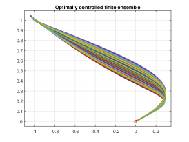
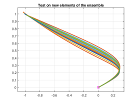
Figure 1. Controlled ensemble. On the left, we reported the optimally controlled trajectories of the sub-ensemble of $\Theta$ obtained by sampling $N=300$ parameters. On the right, we tested the controls obtained before on a new sub-ensemble of $\Theta$, obtained by sampling $20$ new parameters. As we can see, the trajectories belonging to the testing sub-ensemble are correctly steered to the target point $y_{\mathrm{tar}}=(-1,1)^{T}$.

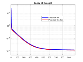
Figure 2. In the graph we reported the decay of the discrete cost achieved by Algorithm 1 (Projected Gradient) and Algorithm 2 (Iterative PMP). As we can see, the performances on this problem are very similar.

Conclusions

In this paper we considered the problem of the optimal control of an ensemble of affine-control systems. We proved the well posedness of the corresponding minimization problem, and we showed with a $\Gamma$-convergence argument how we can reduce the original problem to an approximated one, involving ensembles with a finite number of elements. For these ones, in the case of end-point cost, we proposed two numerical schemes for the approximation of the optimal control. We finally tested the methods on a ensemble optimal control problem in dimension two.

For future development, we plan to study algorithms also for more general costs, and not only for terminal-state penalization. Moreover, we hope to extend the $\Gamma$-convergence results to some proper class of ensembles of nonlinear-control systems. As well as in the affine-control case, we expect that weak topologies on the space of controls are required to have equi-coercivity of the functionals. On the other hand, the challenging aspect is that, in nonlinear-control systems, weakly convergent controls do not induce, in general, locally $C^{0}$-strongly convergent flows.

Appendix A Auxiliary results of Subsection 1.2

Here we prove some auxiliary properties of the mapping $X_{u}:[0,1]\times\Theta\to\mathbb{R}^{n}$, which has been defined in (1.10) for every $u\in\mathcal{U}$. Before proceeding, we recall a version of the Grönwall-Bellman inequality.

Lemma A.1 (Grönwall-Bellman Inequality).

Let $f:[a,b]\to\mathbb{R}_{+}$ be a non-negative continuous function and let us assume that there exists a constant $\alpha>0$ and a non-negative function $\beta\in L^{1}([a,b],\mathbb{R}_{+})$ such that

$$f(s)\leq\alpha+\int_{a}^{s}\beta(\tau)f(\tau)\,d\tau$$

for every $s\in[a,b]$. Then, for every $s\in[a,b]$ the following inequality holds:

$$f(s)\leq\alpha e^{||\beta||_{L^{1}}}.$$ (A.1)

Proof.

This result follows directly from [16, Theorem 5.1]. ∎

We first prove that for every $u\in\mathcal{U}$ the mapping $X_{u}:[0,1]\times\Theta\to\mathbb{R}^{n}$ is bounded.

Lemma A.2.

For every $u\in\mathcal{U}$, let $X_{u}:[0,1]\times\Theta\to\mathbb{R}^{n}$ be the application defined in (1.10) collecting the trajectories of the ensemble of control systems (1.1). Then, for every $R>0$ there exists $C_{R}>0$ such that, if $||u||_{L^{2}}\leq R$, we have

$$|X_{u}(t,\theta)|_{2}\leq C_{R},$$ (A.2)

for every $(t,\theta)\in[0,1]\times\Theta$.

Proof.

Using (1.10), in virtue of the sub-linear growth inequalities (1.5)-(1.6), we observe that

$$|X_{u}(t,\theta)|_{2}=|x^{\theta}_{u}(t)|_{2} \leq|x^{\theta}_{0}|_{2}+\int_{0}^{t}C(1+|x^{\theta}_{u}(\tau)|_{2})(1+|u(\tau)|_{1})\,d\tau$$

$$\leq|x^{\theta}_{0}|_{2}+C(1+\sqrt{k}||u||_{L^{2}})+\int_{0}^{t}C(1+|u(\tau)|_{1})|x^{\theta}_{u}(\tau)|_{2}\,d\tau$$

for every $\theta\in\Theta$ and $t\in[0,1]$. Using Lemma A.1, we deduce that

$$|X(t,\theta)|_{2}\leq\Big{(}|x^{\theta}_{0}|_{2}+C(1+\sqrt{k}||u||_{L^{2}})\Big{)}e^{C\left(1+\sqrt{k}||u||_{L^{2}}\right)}$$

for every $(t,\theta)\in[0,1]\times\Theta$. Recalling the boundedness of $\theta\mapsto x^{\theta}_{0}$ provided by (1.8), the thesis follows from the last inequality. ∎

We shall prove that, when the control $u$ varies in a bounded subset of $\mathcal{U}$, the corresponding functions $X_{u}:[0,1]\times\Theta\to\mathbb{R}^{n}$ that captures the evolution of the ensemble of control systems (1.1) are uniformly equi-continuous on their domain. We first show separately the uniform equi-continuity for the variables in the time domain $[0,1]$ and in the parameter domain $\Theta$. In the next result we observe that the trajectories of the ensemble are Hölder-continuous, uniformly with respect to the parameter $\theta\in\Theta$.

Lemma A.3.

For every $u\in\mathcal{U}$, let $X_{u}:[0,1]\times\Theta\to\mathbb{R}^{n}$ be the application defined in (1.10) collecting the trajectories of the ensemble of control systems (1.1). Then, for every $R>0$ there exists $L_{R}>0$ such that, if $||u||_{L^{2}}\leq R$, then

$$|X_{u}(t_{1},\theta)-X_{u}(t_{2},\theta)|_{2}\leq L_{R}|t_{1}-t_{2}|^{\frac{1}{2}}$$ (A.3)

for every $t_{1},t_{2}\in[0,1]$ and for every $\theta\in\Theta$.

Proof.

Owing to Proposition 1.1 and recalling that $X_{u}(t,\theta)=x^{\theta}_{u}(t)$ for every $(t,\theta)\in[0,1]\times\Theta$ by (1.10), we observe that the thesis follows if we prove that there exists a bounded subset of $H^{1}$ that includes the trajectories $\{x_{u}^{\theta}:[0,1]\to\mathbb{R}^{n}\}_{\theta\in\Theta}$ of (1.1) for every admissible control $u\in\mathcal{U}$ satisfying $||u||_{L^{2}}\leq R$.

From Lemma A.2 we obtain that for every $R>0$ there exists $C_{R}>0$ such that

$$|x_{u}^{\theta}(t)|_{2}\leq C_{R}$$ (A.4)

for every $t\in[0,1]$ and for every $u\in\mathcal{U}$ such that $||u||_{L^{2}}\leq R$. In virtue of Lemma A.2 and the sub-linear inequalities (1.5)-(1.6), we deduce that for every $R>0$ there exists $C_{R}^{\prime}>0$ such that

$$\sup_{\theta\in\Theta}|F_{0}^{\theta}(x_{u}^{\theta}(t))|_{2}\leq C_{R}^{\prime},\qquad\sup_{\theta\in\Theta}\,\sup_{i=1,\ldots,k}|F^{\theta}_{i}(x_{u}^{\theta}(t))|_{2}\leq C_{R}^{\prime}$$

for every $t\in[0,1]$ and for every $u\in\mathcal{U}$ such that $||u||_{L^{2}}\leq R$. Therefore, we have that

$$|\dot{x}^{\theta}_{u}(t)|_{2}\leq C^{\prime}_{R}(1+|u(t)|_{1})$$ (A.5)

for every $t\in[0,1]$, for every $\theta\in\Theta$ and for every $u\in\mathcal{U}$ such that $||u||_{L^{2}}\leq R$. Combining (A.5) and (A.4), we deduce that there exists $C^{\prime\prime}_{R}>0$ such that

$$||x_{u}^{\theta}||_{H^{1}}\leq C^{\prime\prime}_{R}$$

for every $\theta\in\Theta$ and for every $u\in\mathcal{U}$ such that $||u||_{L^{2}}\leq R$. The last inequality and Proposition 1.1 imply that

$$|x^{\theta}_{u}(t_{1})-x^{\theta}_{u}(t_{2})|_{2}\leq L_{R}|t_{1}-t_{2}|^{\frac{1}{2}}$$

for every $t_{1},t_{2}\in[0,1]$, for every $\theta\in\Theta$ and for every $u\in\mathcal{U}$ such that $||u||_{L^{2}}\leq R$, where we set $L_{R}:=\sqrt{C_{R}^{\prime\prime}}$. This establishes (A.3). ∎

Before proceeding, we introduce the modulus of continuity of the function $x_{0}:\Theta\to\mathbb{R}^{n}$ defined in (1.7). Indeed, since $x_{0}:\Theta\to\mathbb{R}^{n}$ is a continuous function defined on a compact domain, it is uniformly continuous, i.e., there exists a non-decreasing function $\omega:\mathbb{R}_{+}\to\mathbb{R}_{+}$ satisfying $0=\omega(0)=\lim_{r\to 0^{+}}\omega(r)$ and such that

$$|x_{0}(\theta_{1})-x_{0}(\theta_{1})|_{2}\leq\omega(|\theta_{1}-\theta_{2}|_{2})$$ (A.6)

for every $\theta_{1},\theta_{2}\in\Theta$.

Lemma A.4.

For every $u\in\mathcal{U}$, let $X_{u}:[0,1]\times\Theta\to\mathbb{R}^{n}$ be the application defined in (1.10) collecting the trajectories of the ensemble of control systems (1.1). Then, for every $R>0$ there exists $\omega_{R}:\mathbb{R}_{+}\to\mathbb{R}_{+}$ such that, if $||u||_{L^{2}}\leq R$, then

$$|X_{u}(t,\theta_{1})-X_{u}(t,\theta_{2})|_{2}\leq\omega_{R}(|\theta_{1}-\theta_{2}|_{2})$$ (A.7)

for every $t\in[0,1]$ and for every $\theta_{1},\theta_{2}\in\Theta$, where $\omega_{R}$ is a non-decreasing function that satisfies $\omega(0)=\lim_{r\to 0^{+}}\omega_{R}(r)=0$.

Proof.

Recalling (1.10), we compute

$$|X_{u}(t,\theta_{1})-X_{u}(t,\theta_{2})|_{2} =|x_{u}^{\theta_{1}}(t)-x_{u}^{\theta_{2}}(t)|_{2}$$

$$\leq|x_{0}(\theta_{1})-x_{0}(\theta_{2})|_{2}+\int_{0}^{t}|F_{0}^{\theta_{1}}(x_{u}^{\theta_{1}}(\tau))-F_{0}^{\theta_{2}}(x_{u}^{\theta_{2}}(\tau))|_{2}\,d\tau$$

$$\qquad+\int_{0}^{t}\sum_{i=1}^{k}\left(|F^{\theta_{1}}_{i}(x_{u}^{\theta_{1}}(\tau))-F^{\theta_{2}}_{i}(x_{u}^{\theta_{2}}(\tau))|_{2}|u_{i}(\tau)|\right)d\tau$$

for every $t\in[0,1]$, for every $\theta_{1},\theta_{2}\in\Theta$ and for every $u\in\mathcal{U}$. Using (1.2) and the Lipschitz-continuity conditions (1.3)-(1.4), the last expression yields

$$|x_{u}^{\theta_{1}}(t)-x_{u}^{\theta_{2}}(t)|_{2} \leq|x_{0}(\theta_{1})-x_{0}(\theta_{2})|_{2}$$

$$\qquad+\int_{0}^{t}L(1+|u(\tau)|_{1})\left(|x_{u}^{\theta_{1}}(\tau)-x_{u}^{\theta_{2}}(\tau)|_{2}+|\theta_{1}-\theta_{2}|_{2}\right)d\tau$$

$$\leq|x_{0}(\theta_{1})-x_{0}(\theta_{2})|_{2}+L(1+\sqrt{k}||u||_{L^{2}})|\theta_{1}-\theta_{2}|_{2}$$

$$\qquad+\int_{0}^{t}L(1+|u(\tau)|_{1})(|x_{u}^{\theta_{1}}(\tau)-x_{u}^{\theta_{2}}(\tau)|_{2})\,d\tau$$

for every $t\in[0,1]$, for every $\theta_{1},\theta_{2}\in\Theta$ and for every $u\in\mathcal{U}$. Owing to Lemma A.1, from the last inequality we deduce that (A.7) holds for every $t\in[0,1]$, for every $\theta_{1},\theta_{2}\in\Theta$ and for every $u\in\mathcal{U}$ with $||u||_{L^{2}}\leq R$, where the function $\omega_{R}:\mathbb{R}_{+}\to\mathbb{R}_{+}$ is defined as follows:

$$\omega_{R}(r):=e^{L\left(1+\sqrt{k}R\right)}\left(\omega(r)+L(1+\sqrt{k}R)r\right),$$

and $\omega:\mathbb{R}_{+}\to\mathbb{R}_{+}$ is a modulus of continuity for the mapping $x_{0}:\Theta\to\mathbb{R}^{n}$ (see (A.6)). ∎

We are now in position of stating the uniform equi-continuity result.

Lemma A.5.

For every $u\in\mathcal{U}$, let $X_{u}:[0,1]\times\Theta\to\mathbb{R}^{n}$ be the application defined in (1.10) collecting the trajectories of the ensemble of control systems (1.1). Then, for every $R>0$ there exists $L_{R}>0$ and $\omega_{R}:\mathbb{R}_{+}\to\mathbb{R}_{+}$ such that, if $||u||_{L^{2}}\leq R$, then

$$|X_{u}(t_{1},\theta_{1})-X_{u}(t_{2},\theta_{2})|_{2}\leq L_{R}|t_{1}-t_{2}|^{\frac{1}{2}}+\omega_{R}(|\theta_{1}-\theta_{2}|_{2})$$ (A.8)

for every $(t_{1},\theta_{1}),(t_{2},\theta_{2})\in[0,1]\times\Theta$, where $\omega_{R}$ is a non-decreasing function satisfying $\omega(0)=\lim_{r\to 0^{+}}\omega_{R}(r)=0$.

Proof.

The thesis (A.8) follows directly from the triangular inequality and from Lemma A.3 and Lemma A.4. ∎

Appendix B Auxiliary results of Subsection 1.3

Here we establish some auxiliary results concerning the mapping $\Lambda_{u}$ defined in (1.19). We use the same scheme used in Appendix A, and we first show that $\Lambda_{u}$ is bounded.

Lemma B.1.

Let us assume that the mappings $(x,\theta)\mapsto\frac{\partial}{\partial x}F_{i}(x,\theta)$ are continuous for every $i=0,\ldots,k$, as well as the gradient $(x,\theta)\mapsto\nabla_{x}a(x,\theta)$. For every $u\in\mathcal{U}$, let $\Lambda_{u}:[0,1]\times\Theta\to(\mathbb{R}^{n})^{*}$ be the application defined in (1.19). Then, for every $R>0$ there exists $C_{R}>0$ such that, if $||u||_{L^{2}}\leq R$, we have

$$|\Lambda_{u}(t,\theta)|_{2}\leq C_{R},$$ (B.1)

for every $(t,\theta)\in[0,1]\times\Theta$.

Proof.

We preliminarily observe that, owing to Lemma A.2 and the continuity of $\nabla_{x}a$, there exists $C_{R}^{1}>0$ such that

$$\sup_{\theta\in\Theta}|\nabla_{x}a(X_{u}(t,\theta),\theta)|_{2}\leq C_{R}^{1}.$$

From the definition of $\Lambda_{u}:[0,1]\times\Theta\to(\mathbb{R}^{n})^{*}$ in (1.19), it follows that

$$\begin{split}|\Lambda_{u}(t,\theta)|_{2}=|\lambda_{u}^{\theta}(t)|_{2}&\leq|\lambda_{u}^{\theta}(1)|_{2}+\int_{t}^{1}|\lambda_{u}^{\theta}(\tau)|_{2}\left|\frac{\partial F_{0}(x_{u}^{\theta}(\tau),\theta)}{\partial x}+\sum_{i=1}^{k}u_{i}(\tau)\frac{\partial F_{i}(x_{u}^{\theta}(\tau),\theta)}{\partial x}\right|_{2}\,d\tau\\ &\leq|\lambda_{u}^{\theta}(1)|_{2}+\int_{t}^{1}|\lambda_{u}^{\theta}(\tau)|_{2}L(1+|u(\tau)|_{1})\,d\tau\end{split}$$

for every $(t,\theta)\in[0,1]\times\Theta$, where we used (1.3)-(1.4) in the last passage. Finally, combining the previous inequality with Lemma A.1 and (1.11), we deduce (B.1). ∎

In the next lemma we show that $\Lambda_{u}$ is Hölder-continuous in time.

Lemma B.2.

Let us assume that the mappings $(x,\theta)\mapsto\frac{\partial}{\partial x}F_{i}(x,\theta)$ are continuous for every $i=0,\ldots,k$, as well as the gradient $(x,\theta)\mapsto\nabla_{x}a(x,\theta)$. For every $u\in\mathcal{U}$, let $\Lambda_{u}:[0,1]\times\Theta\to(\mathbb{R}^{n})^{*}$ be the application defined in (1.19). Then, for every $R>0$ there exists $L_{R}>0$ such that, if $||u||_{L^{2}}\leq R$, then

$$|\Lambda_{u}(t_{1},\theta)-\Lambda_{u}(t_{2},\theta)|_{2}\leq L_{R}|t_{1}-t_{2}|^{\frac{1}{2}}$$ (B.2)

for every $t_{1},t_{2}\in[0,1]$ and for every $\theta\in\Theta$.

Proof.

We recall that by the definition (1.19) we have $\Lambda_{u}(\cdot,\theta)=\lambda_{u}^{\theta}(\cdot)$, for every $\theta\in\Theta$, where $\lambda_{u}^{\theta}:[0,1]\to(\mathbb{R}^{n})^{*}$ solves the linear differential equation (1.18). Therefore, we employ the same strategy as in the proof of Lemma A.3, i.e., we show that there exists a bounded subset of $H^{1}$ that includes the family of curves $\{\lambda_{u}^{\theta}:[0,1]\to(\mathbb{R}^{n})^{*}\}_{\theta\in\Theta}$ for every admissible control $u\in\mathcal{U}$ satisfying $||u||_{L^{2}}\leq R$. From Lemma B.1 it descends that there exists $C_{R}>0$ such that

$$|\lambda_{u}^{\theta}(t)|_{2}=|\Lambda_{u}(t,\theta)|_{2}\leq C_{R}$$ (B.3)

for every $t\in[0,1]$ and $\theta\in\Theta$. On the other hand, we compute

$$\begin{split}|\dot{\lambda}_{u}^{\theta}(t)|_{2}&\leq|\lambda_{u}^{\theta}(t)|_{2}\left|\frac{\partial F_{0}(x_{u}^{\theta}(t),\theta)}{\partial x}+\sum_{i=1}^{k}u_{i}(t)\frac{\partial F_{i}(x_{u}^{\theta}(t),\theta)}{\partial x}\right|_{2}\\ &\leq C_{R}L(1+|u(t)|_{1})\end{split}$$ (B.4)

for a.e. $t\in[0,1]$ and for every $\theta\in\Theta$. Hence, combining (B.3)-(B.4) with (1.11) and Proposition 1.1, we deduce (B.2). ∎

In the following result we prove the uniform continuity of $\Lambda_{u}:[0,1]\times\Theta\to(\mathbb{R}^{n})^{*}$ with respect to the second variable.

Lemma B.3.

Let us assume that the mappings $(x,\theta)\mapsto\frac{\partial}{\partial x}F_{i}(x,\theta)$ are continuous for every $i=0,\ldots,k$, as well as the gradient $(x,\theta)\mapsto\nabla_{x}a(x,\theta)$. For every $u\in\mathcal{U}$, let $\Lambda_{u}:[0,1]\times\Theta\to(\mathbb{R}^{n})^{*}$ be the application defined in (1.19). Then, for every $R>0$ there exists $\omega_{R}:\mathbb{R}_{+}\to\mathbb{R}_{+}$ such that, if $||u||_{L^{2}}\leq R$, then

$$|\Lambda_{u}(t,\theta_{1})-\Lambda_{u}(t,\theta_{2})|_{2}\leq\omega_{R}(|\theta_{1}-\theta_{2}|_{2})$$ (B.5)

for every $t\in[0,1]$ and for every $\theta_{1},\theta_{2}\in\Theta$, where $\omega_{R}$ is a non-decreasing function that satisfies $\omega(0)=\lim_{r\to 0^{+}}\omega_{R}(r)=0$.

Proof.

From the definition (1.19) and from (1.18), it follows that

$$\begin{split}|\Lambda_{u}(t,\theta_{1})&-\Lambda_{u}(t,\theta_{2})|_{2}=|\lambda_{u}^{\theta_{1}}(t)-\lambda_{u}^{\theta_{2}}(t)|_{2}\\ &\leq|\nabla_{x}a(x_{u}^{\theta_{1}}(1),\theta_{1})-\nabla_{x}a(x_{u}^{\theta_{2}}(1),\theta_{2})|_{2}\\ &\quad+\int_{t}^{1}|\lambda_{u}^{\theta_{2}}(\tau)|_{2}\left(\left|\frac{\partial F_{0}(x_{u}^{\theta_{1}}(\tau),\theta_{1})}{\partial x}-\frac{\partial F_{0}(x_{u}^{\theta_{2}}(\tau),\theta_{2})}{\partial x}\right|_{2}\right.\\ &\qquad\qquad\qquad\qquad\quad\left.+\sum_{i=1}^{k}|u_{i}(\tau)|\left|\frac{\partial F_{i}(x_{u}^{\theta_{1}}(\tau),\theta_{1})}{\partial x}-\frac{\partial F_{i}(x_{u}^{\theta_{2}}(\tau),\theta_{2})}{\partial x}\right|_{2}\right)\,d\tau\\ &\quad+\int_{t}^{1}|\lambda_{u}^{\theta_{1}}(\tau)-\lambda_{u}^{\theta_{2}}(\tau)|_{2}\left|\frac{\partial F_{0}(x_{u}^{\theta_{1}}(\tau),\theta_{1})}{\partial x}+\sum_{i=1}^{k}u_{i}(\tau)\frac{\partial F_{i}(x_{u}^{\theta_{1}}(\tau),\theta_{1})}{\partial x}\right|_{2}\,d\tau\end{split}$$ (B.6)

for every $t\in[0,1]$ and for every $\theta_{1},\theta_{2}\in\Theta$. In virtue of Lemma A.2, there exists a compact set $K_{R}\subset\mathbb{R}^{n}$ such that the image $X_{u}([0,1],\Theta)\subset K_{R}$ for every $u\in\mathcal{U}$ with $||u||_{L^{2}}\leq R$. The continuity assumptions guarantee that $(x,\theta)\mapsto\frac{\partial}{\partial x}F_{i}(x,\theta)$ for $i=0,\ldots,k$ and $(x,\theta)\mapsto\nabla_{x}a(x,\theta)$ are uniformly continuous when restricted to $K_{R}\times\Theta$. Moreover, in virtue of Lemma A.4, we deduce that the applications defined as $\theta\mapsto\frac{\partial}{\partial x}F_{i}(X_{u}(t,\theta),\theta)$ for $i=0,\ldots,k$ and $\theta\mapsto\nabla_{x}a(X_{u}(1,\theta),\theta)$ are uniformly equi-continuous for every choice of $t\in[0,1]$ and $u\in\mathcal{U}$ with $||u||_{L^{2}}\leq R$. Let $\omega^{\prime}_{R}:\mathbb{R}_{+}\to\mathbb{R}_{+}$ be a modulus of continuity for all these functions. Hence, using Lemma B.1, from (B.6) we obtain that there exists $C_{R}>0$ such that

$$\begin{split}|\Lambda_{u}(t,\theta_{1})-\Lambda_{u}(t,\theta_{2})|_{2}&=|\lambda_{u}^{\theta_{1}}(t)-\lambda_{u}^{\theta_{2}}(t)|_{2}\\ &\leq\omega^{\prime}_{R}(|\theta_{1}-\theta_{2}|_{2})+C_{R}(1+||u||_{L^{1}})\omega^{\prime}_{R}(|\theta_{1}-\theta_{2}|_{2})\\ &\quad+C_{R}\int_{t}^{1}|\lambda_{u}^{\theta_{1}}(\tau)-\lambda_{u}^{\theta_{2}}(\tau)|_{2}\left(1+\sum_{i=1}^{k}|u_{i}(\tau)|\right)\,d\tau\end{split}$$

for every $t\in[0,1]$, for every $\theta_{1},\theta_{2}\in\Theta$ and for every $u\in\mathcal{U}$ with $||u||_{L^{2}}\leq R$. Then, the thesis (B.5) follows directly from Lemma A.1. ∎

Finally, the next results proves the uniform continuity of $\Lambda_{u}$.

Lemma B.4.

Let us assume that the mappings $(x,\theta)\mapsto\frac{\partial}{\partial x}F_{i}(x,\theta)$ are continuous for every $i=0,\ldots,k$, as well as the gradient $(x,\theta)\mapsto\nabla_{x}a(x,\theta)$. For every $u\in\mathcal{U}$, let $\Lambda_{u}:[0,1]\times\Theta\to(\mathbb{R}^{n})^{*}$ be the application defined in (1.19). Then, for every $R>0$ there exists $L_{R}>0$ and $\omega_{R}:\mathbb{R}_{+}\to\mathbb{R}_{+}$ such that, if $||u||_{L^{2}}\leq R$, then

$$|\Lambda_{u}(t_{1},\theta_{1})-\Lambda_{u}(t_{2},\theta_{2})|_{2}\leq L_{R}|t_{1}-t_{2}|^{\frac{1}{2}}+\omega_{R}(|\theta_{1}-\theta_{2}|_{2})$$ (B.7)

for every $(t_{1},\theta_{1}),(t_{2},\theta_{2})\in[0,1]\times\Theta$, where $\omega_{R}$ is a non-decreasing function satisfying $\omega(0)=\lim_{r\to 0^{+}}\omega_{R}(r)=0$.

Proof.

The thesis (B.7) follows directly from the triangular inequality and from Lemma B.2 and Lemma B.3. ∎

(A. Scagliotti).

“School of Computation, Information and Technology”,
TU Munich, Garching b. München, Germany.

Munich Center for Machine Learning (MCML), Germany.

Email address: scag -at- ma.tum.de

References

- [1] A. Agrachev, Yu. Sachkov. Control Theory from the Geometric Viewpoint. Encyclopaedia of Mathematical Sciences, Springer-Verlag Berlin Heidelberg (2004). doi: 10.1007/978-3-662-06404-7
- [2] A. Agrachev, Y. Baryshnikov, A. Sarychev. Ensemble controllability by Lie algebraic methods. ESAIM: Cont., Opt. and Calc. Var., 22:921-938 (2016). doi: 10.1051/cocv/2016029
- [3] N. Augier, U. Boscain, M. Sigalotti. Adiabatic ensemble control of a continuum of quantum systems. SIAM J. Control Optim., 56(6):4045-4068 (2018). doi: 10.1137/17M1140327
- [4] K. Beauchard, J.-M. Coron, P. Rouchon. Controllability issues for continuousspectrum systems and ensemble controllability of Bloch equations Comm. Math. Phys., 296(2):525-557 (2010). doi: 10.1007/s00220-010-1008-9
- [5] M. Belhadj, J. Salomon, G. Turinici. Ensemble controllability and discrimination of perturbed bilinear control systems on connected, simple, compact Lie groups. Eur. J. Control, 22:23-29 (2015). doi: 10.1016/j.ejcon.2014.12.003
- [6] P. Bettiol, N. Khalil. Necessary optimality conditions for average cost minimization problems. Discete Contin. Dyn. Syst. - B., 24(5): 2093-2124 (2019). doi: 10.3934/dcdsb.2019086
- [7] B. Bonnet, C. Cipriani, M. Fornasier, H. Huang. A measure theoretical approach to the mean-field maximum principle for training NeurODEs. Nonlinear Analysis, 227: 113-161 (2023). doi: 10.1016/j.na.2022.113161
- [8] H. Brezis. Functional Analysis, Sobolev Spaces and Partial Differential Equations. Universitext, Springer New York NY (2011). doi: 10.1007/978-0-387-70914-7
- [9] R.W. Brockett. On the control of a flock by a leader. Proc. Steklov Inst. Math., 268:49-57 (2010). doi: 10.1134/S0081543810010050
- [10] F. Chernousko, A. Lyubushin. Method of successive approximations for solution of optimal control problems. Opt. Control Appl. Methods, 3(2):101-114 (1982).
- [11] F.C. Chittaro, J.P. Gauthier. Asymptotic ensemble stabilizability of the Bloch equation. Sys. Control Lett., 113:36-44 (2018). doi: 10.1016/j.sysconle.2018.01.008
- [12] E. Çinlar. Probability and Stochastics. Graduate Texts in Mathematics, Springer-Verlag, New York (2010). doi: 10.1007/978-0-387-87859-1
- [13] G. Dirr, M. Schönlein. Uniform and -ensemble reachability of parameter-dependent linear systems J. Differ. Eq., 283:216-262 (2021). doi: 10.1016/j.jde.2021.02.032
- [14] J. Daleckii, M. Krein. Stability of solutions of differential equations in Banach space. Translations of Mathematical Monographs, American Mathematical Soc. (1974).
- [15] G. Dal Maso. An Introduction to -convergence. Progress in nonlinear differential equations and their applications, Birkhäuser Boston MA (1993).
- [16] S. Ethier, T. Kurtz. Markov Processes: Characterization and Convergence. Wiley series in probability and statistics, John Wiley & Sons New York (1986).
- [17] J. Hale. Ordinary Differential Equations. Krieger Publishing Company (1980).
- [18] P. Lambrianides, Q. Gong, D. Venturi. A new scalable algorithm for computational optimal control under uncertainty. J. Comput. Phys., 420 (2020). doi: 10.1016/j.jcp.2020.109710
- [19] J.-S Li, N. Khaneja. Control of inhomogeneous quantum ensembles, Phys. Rev. A, 73(3) (2006). doi: 10.1103/PhysRevA.73.030302
- [20] J.-S Li, N. Khaneja. Ensemble control of Bloch equations. IEEE Transat. Automat. Control, 54:528-536 (2009). doi: 10.1109/TAC.2009.2012983
- [21] R. Murray, M. Palladino. A model for system uncertainty in reinforcement learning. Syst. Control Lett., 122:24-31 (2018). doi: 10.1016/j.sysconle.2018.09.011
- [22] Q. Mérigot, F. Santambrogio, C. Sarrazin. Non-asymptotic convergence bounds for Wasserstein approximation using point clouds. Adv. Neur. Inf. Process Syst., 34:12810-12821 (2021).
- [23] Yu. Nesterov. Lectures on Convex Optimization. Springer Optimization, Springer Nature Switzerland AG (2018). doi: 10.1007/978-3-319-91578-4
- [24] A. Pacifico, A. Pesare, M. Falcone. A New Algorithm for the LQR Problem with Partially Unknown Dynamics. In: Large-Scale Scientific Computing 2021. Lecture Notes in Computer Science, vol 13127, Springer (2022). doi: 10.1007/978-3-030-97549-4_37
- [25] A. Pesare, M. Palladino, M. Falcone. Convergence of the Value Function in Optimal Control Problems with Unknown Dynamics. 2021 European Control Conference (ECC), pp. 2426-2431 (2021). doi: 10.23919/ECC54610.2021.9655079
- [26] A. Pesare, M. Palladino, M. Falcone. Convergence results for an averaged LQR problem with applications to Reinforcement Learning. Math. Control Signals Syst., 33:379–411 (2021). doi: 10.1007/s00498-021-00294-y
- [27] C. Phelps, J.O. Royset, Q. Gong. Optimal control of uncertain systems using sample average approximations. SIAM J. Control Optim., 54(1): 1-29 (2016). doi: 10.1137/140983161
- [28] J. Ruths, J.-S. Li. Optimal control of inhomogenous ensembles. IEEE Trans. Aut. Control, 57(8):2021-2032 (2012). doi: 10.1109/TAC.2012.2195920
- [29] Y. Sakawa, Y. Shindo. On global convergence of an algorithm for optimal control. IEEE Trans. Automat. Contr., 25(6):1149-1153 (1980).
- [30] A. Scagliotti. A gradient flow equation for optimal control problems with end-point cost. J. Dyn. Control Syst., (2022). doi: 10.1007/s10883-022-09604-2
- [31] A. Scagliotti. Deep Learning approximation of diffeomorphisms via linear-control systems. Math. Control Relat. Fields (2022). doi: 10.3934/mcrf.2022036
- [32] R. Triggiani. Controllability and observability in Banach spaces with bounded operators. SIAM J. Control, 13(2): 462-491 (1975). doi: 10.1137/0313028
- [33] R. B. Vinter. Minimax Optimal Control. SIAM J. Control Optim., 44(3): 939-968 (2005). doi: 10.1137/S0363012902415244