A phase-field model for ferroelectrics with general kinetics.
Part I: Model formulation

Abstract

When subjected to electro-mechanical loading, ferroelectrics see their polarization evolve through the nucleation and evolution of domains. Existing mesoscale phase-field models for ferroelectrics are typically based on a gradient-descent law for the evolution of the order parameter. While this implicitly assumes that domain walls evolve with linear kinetics, experiments instead indicate that domain wall kinetics is nonlinear. This, in turn, is an important feature for the modeling of rate-dependent effects in polarization switching. We propose a new multiple-phase-field model for ferroelectrics, which permits domain wall motion with nonlinear kinetics, with applications in other solid-solid phase transformation problems. By means of analytical traveling wave solutions, we characterize the interfacial properties (energy and width) and the interface kinetics of straight domain walls, as furnished by the general kinetics model, and compare them to those of the classical Allen–Cahn model. We show that the proposed model propagates domain walls with arbitrarily chosen nonlinear kinetic relations, which can be tuned to differ for the different types of domain walls in accordance with experimental evidence.

1 Introduction

Ferroelectrics are a prime example of multifunctional materials with electro-mechanical coupling. They are largely used as sensors and actuators for their piezoelectric properties (Uchino, 2018) as well as in ferroelectric random-access memory (Ishiwara et al., 2004), which uses the reversibility of spontaneous polarization states. Below a critical temperature, referred to as the Curie temperature, ferroelectric ceramics possess a polar structure with a spontaneous electric polarization, which can be reversed under the application of electro-mechanical loading. Polarization switching is accommodated by transformations between lattice variants of different orientations—e.g., the six orientations of the tetragonal variants for barium titanate (BaTiO₃) at room temperature—and between phases of distinct crystal symmetry types—e.g., the tetragonal and rhombohedral phases in some compositions of lead zirconate titanate (PZT).

At the mesoscale (tens of nanometers to hundreds of microns), polarization reversal occurs through the emergence and evolution of a microstructure formed by the different variants (and phases, where applicable) referred to as ferroelectric domains separated by domain walls. In defect-free ferroelectric single-crystals, the microstructure that develops during switching vanishes at the end of that process, which leads to a single polarization domain in the sample (Little, 1955). By contrast, in polycrystalline ferroelectric ceramics, grains with different orientations exert mechanical constraints, so that microstructural arrangements with multiple ferroelectric domains remain after polarization switching (Arlt and Sasko, 1980).

At the macroscale, a few representative curves are commonly used to characterize polarization switching. First, bipolar measurements are obtained by cycling the applied electric field between $\pm e_{\max}$. These yield the $p$-$e$ hysteresis curve and the strain butterfly curve, giving, respectively, the evolution of the average polarization and longitudinal strain (under stress-free conditions) as functions of the applied electric field. When bipolar measurements are performed at a sufficiently low rate (typically with frequency $\omega\lesssim 10^{-3}\,\mathrm{Hz}$), no rate dependence is observed, suggesting that the kinetics of domain evolution only plays a minor role. By contrast, at higher rates, bipolar curves show a strong rate dependence, a consequence of the finite kinetics of domain evolution (see, e.g., Wieder 1957; Chen et al. 2011 and Wieder 1957; Schmidt 1981; Yin and Cao 2002; Chen et al. 2011; Kannan et al. 2022 for rate-dependent hysteresis curves in single and polycrystals, respectively). Another type of experiment, referred to as pulse experiment, determines the time evolution of the average polarization and strain in response to an applied pulse of the electric field (see, e.g., Merz 1954, 1956; Hubmann et al. 2016 for single crystals and Genenko et al. 2012; Schultheiß et al. 2018, 2019 for polycrystals). While no significant polarization reversal occurs during the short rise time of pulse loading ($\sim 0.1\,\mu\mathrm{s}$), polarization switching does occur during the subsequent constant applied electric field. Overall, the profile of the time evolution of polarization and strain is a fingerprint at the macroscale of the sequence of switching mechanisms at the mesoscale, namely, the nucleation of domains and their subsequent evolution with finite kinetics. Hence, a proper modeling of the kinetics of domain evolution is crucial for understanding the macroscopic response of ferroelectrics as given by rate-dependent bipolar measurements or pulse experiments.

At the mesoscale, continuum models that resolve the time evolution of the domain microstructure together with the local distribution of electric and mechanical fields are of two sorts: (i) sharp-interface models, which describe domain walls as surfaces of discontinuity with zero thickness, and (ii) diffuse-interface models (also referred to as phase-field models), in which the electro-mechanical fields vary steeply but continuously across domain walls.

In sharp-interface models, the classical balance laws of electro-quasistatics and mechanics provide field equations within ferroelectric domains and jump conditions at the domain walls. These are completed by constitutive relations that account for the elastic, dielectric, and piezoelectric properties of the ferroelectric variants. Domain walls are twin interfaces or phase boundaries, for which it is known from the continuum theory of phase transitions that their velocity is, in the subsonic regime, not uniquely determined by the above system of equations (Abeyaratne and Knowles, 2006). Hence, the jump conditions are complemented by an additional relation termed the kinetic relation between the normal velocity of the interface and the local driving traction. This framework, first developed in the mechanics literature within the thermo-mechanical setting (Truskinovsky, 1987; Abeyaratne and Knowles, 1990), was later extended to include the interaction with electromagnetic fields (Jiang, 1994b) and applied to ferroelectrics in Jiang (1994a); Rosakis and Jiang (1995); Loge and Suo (1996); Kessler and Balke (2006). Nevertheless, due to the presence of moving surfaces of discontinuity, the sharp-interface model does not lend itself to numerical simulations, which is why in practice its use is limited to analytical works.

In parallel, diffuse-interface approaches based on the time-dependent Ginzburg-Landau (TDGL) model were developed to simulate the evolution of the patterns formed by ferroelectric domains. Based on the early modeling of the structure of domains in ferromagnets by Landau and Lifshitz (1935), Ginzburg-Landau potentials—with multiwelled functions of the polarization vector supplemented with polarization gradient terms—were used to model the dependence on temperature of properties of ferroelectric domain walls, such as their thickness and energy, when close to the paralectric-ferroelectric transition temperature (Zhirnov, 1959; Bulaevskii and Ginzburg, 1964; Cao and Cross, 1991). Later, and initially in the physics and material science literature, these works were extended by the TDGL formulation with the purpose of investigating the paraelectric–ferroelectric transition with a focus on the velocity of the paraelectric–ferroelectric interface (Gordon, 1986) and the formation and evolution of patterns formed by the different tetragonal variants. The latter arise in ferroelectrics quenched below the Curie temperature, as a consequence of the paraelectric–ferroelectric transition (Nambu and Sagala, 1994; Ahluwalia and Cao, 2001; Yang and Chen, 1995; Hu and Chen, 1997, 1998; Li et al., 2001). Afterwards, works in the the mechanics literature dealt with the coupling of the TDGL equations—which were re-derived from variational principles (Zhang and Bhattacharya, 2005a) or microforce balance (Su and Landis, 2007)—with electrostatic Gauss’ law and the mechanical balance equations to simulate the evolution of ferroelectric domain patterns in response to an applied electric field, i.e., polarization switching (Zhang and Bhattacharya, 2005a, b; Su and Landis, 2007; Vidyasagar et al., 2017; Indergand et al., 2020).

While these later works successfully accounted for features of the quasistatic $p$-$e$-hysteresis and strain butterfly curves, the TDGL model reaches its limitations when it comes to modeling rate effects as well as the material response to pulse switching experiments. For instance, TDGL simulations of polarization switching in response to applied electric field pulses of magnitude $e_{\text{sw}}$ yield a switching time $\tau_{s}$ that scales as $\tau_{s}\propto 1/e_{\text{sw}}$ (Indergand, 2019) in contradiction to the experimental scaling $\tau_{s}\propto\mathrm{e}^{1/e_{\text{sw}}}$ (Merz, 1956; Schultheiß et al., 2019), known as Merz law.

The above scaling that results from the TDGL model is expected, since the TDGL formulation postulates a linear relation between the time evolution of the order parameter (polarization $\bm{p}$) and the (negative of the) variational derivative of the free-energy density $\Psi$, i.e.,

$$\mu\dot{\bm{p}}=-\frac{\delta\Psi}{\delta\bm{p}}$$ (1.1)

with the inverse mobility coefficient $\mu>0$. As will be discussed in Section 3, when the TDGL model is viewed as the regularization of a sharp-interface model, the evolution law (1.1), also known as the Allen–Cahn equation (Allen and Cahn, 1979), amounts to assuming a linear kinetic relation. As reviewed in A, this point is precisely in contrast with experimental evidence, which shows that domain wall motion is governed by nonlinear kinetic relations. Hence, modeling time-dependent switching with a diffuse-interface approach requires a new phase-field formulation, one that permits nonlinear domain wall kinetics. This is the objective of the present work, which focuses on the theoretical foundation. Part II of this study will present numerical applications.

Domain evolution in ferroelectrics is a specific case of the general class of problems of structural phase transformations. These include, e.g., stress-induced phase transformations (such as the martensite–austenite transformation) and deformation twinning. In this more general setting, the question of how to formulate a regularized model that accounts for the nonlinear kinetics of interfaces in solids was considered before. Hou et al. (1999) used a level-set method based on the Hamilton-Jacobi equation (Osher and Sethian, 1988) to model interface propagation with nonlinear and anisotropic kinetics. Alber and Zhu (2013) proposed a phase-field model for two-phase solid-solid transformations—termed the hybrid model because it shares properties of a Hamilton-Jacobi and a parabolic equation—which permits nonlinear kinetics (see also Alber and Zhu, 2005, 2007). The model proposed in Section 4 of this article may be interpreted as a reformulation of that of Alber and Zhu (2013), which is specialized for ferroelectrics and extended to transformations between multiple phases (as opposed to only two in the works of Alber and Zhu (2005, 2007, 2013)). On a different front, Agrawal and Dayal (2015a, b) recently proposed a phase-field model that admits nonlinear kinetics. Their evolution equation closely resembles the one of Hou et al. (1999), reformulated as a phase-field model instead of a level-set method. However, the model of Agrawal and Dayal (2015a) does not lend itself easily to extensions to multiple phases (see Agrawal (2016)). Finally, Tůma et al. (2018) included a mixed-type dissipation potential—combining viscous and rate-independent contributions—in the variational formulation of a phase-field model for displacive phase transformations such as martensitic transformations. This furnishes a nonlinear kinetic law in the corresponding sharp-interface model, one that prescribes a threshold on the driving force for interface motion. This model was later extended by including this feature in a multi-phase-field model for solid-solid transformations, which rests upon a micromorphic formulation (Rezaee-Hajidehi and Stupkiewicz, 2021). While these two formulations introduce in a neat fashion a specific nonlinearity in the kinetic relation (specifically, a threshold on the driving force), our goal here is to include a kinetic relation with general nonlinearity so as to accurately account for experimentally measured kinetics. Within this setting of diffuse-interface models with nonlinear kinetics for solid-solid transformations, the one we introduce in Section 4 is the first to encompass multiple-phase transformations and embed arbitrary nonlinearity. It finds a particularly relevant application in ferroelectric domain evolution, since experimental evidence confirms that the kinetic relation for domain walls is nonlinear. Further, the proposed model allows to select different kinetics for the different types of domain walls (e.g., 90^∘ and 180^∘ domain walls in tetragonal ferroelectrics), as it is indicated by experimental results.

The remainder of this article is organized as follows. In Section 2 we introduce a sharp-interface model for ferroelectrics, which constitutes the basis for discussing the characteristics of the diffuse-interface models of subsequent sections. Section 3 reviews the characteristics of classical models based on the Allen–Cahn equation with regards to the properties (interfacial energy and thickness) and kinetics of 90^∘ and 180^∘ domain walls. In Section 4, we introduce a new phase-field model for ferroelectrics with general kinetics, and we discuss its properties with focus on the kinetics of the two types of domain walls. The main features of the new phase-field model are discussed in the conclusion in Section 5. Empirical data on the nonlinear kinetics of domain walls in barium titanate coming from the physics literature are briefly reviewed in A. Numerical applications will be reported in Part II of this study.

2 The sharp-interface model for ferroelectrics

We begin by formulating a mesoscale continuum model for ferroelectrics. Domain walls are represented by sharp interfaces, across which some or all of the electro-mechanical fields exhibit discontinuities. The motion of a domain wall is governed by a function, termed the kinetic relation, which relates its normal velocity to the thermodynamic driving traction exerted on the interface. The sharp-interface model introduced in this section serves as a reference to discuss the behavior of the diffuse-interface models of Sections 3 and 4.

In Section 2.1, we present the mechanical balance laws, Maxwell’s equations and evolution equation for a singular surface, formulated for a general continuum subject to electro-mechanical coupling. In Section 2.2, we introduce an expression for the electric enthalpy of ferroelectrics, from which the constitutive relations derive, and we discuss the functional form of the kinetic relation appropriate for domain wall motion in ferroelectrics. The resulting model is specialized to rigid ferroelectrics in Section 2.3.

Note that we use the following notation of tensor calculus. For any vector fields $\bm{v}(\bm{x},t)$ and $\bm{w}(\bm{x},t)$, second-order tensor fields $\bm{R}(\bm{x},t)$ and $\bm{S}(\bm{x},t)$, and third- and fourth-order tensors $\mathbb{T}$ and $\mathbb{U}$, respectively, we have in a Cartesian basis

$$\begin{aligned} &(\nabla\bm{v})_{ij}=v_{i,j},\quad&(\operatorname{div}\bm{R})_{i}=R_{ij,j},\quad&(\bm{R}\bm{v})_{i}=R_{ij}v_{j},\quad&(\bm{R}\cdot\bm{S})_{ij}=R_{ik}S_{kj},\\ &\bm{R}:\bm{S}=R_{ij}S_{ij},\quad&(\mathbb{T}^{\mathrm{T}}\cdot\bm{v})_{ij}=T_{kij}v_{k},\quad&(\mathbb{T}:\bm{R})_{k}=T_{ijk}R_{jk},\quad&(\mathbb{U}:\bm{R})_{ij}=U_{ijkl}R_{kl},\end{aligned}$$ (2.1)

where indices following a comma indicate spatial derivatives, and we use Einstein’s summation convention.

2.1 General principles

We consider a deformable body $\mathcal{B}$ occupying the region $\Omega\subset\mathbb{R}^{3}$ in the presence of electrostatic fields filling $\mathbb{R}^{3}$. The deformation of $\mathcal{B}$ is described by the displacement field $\bm{u}(x,t):\Omega\times\mathbb{R}\rightarrow\mathbb{R}^{3}$. Given the small strains encountered in ferroelectric ceramics, we assume linearized kinematics and introduce the infinitesimal strain tensor $\bm{\varepsilon}(\bm{x},t)=(\nabla\bm{u})_{\mathrm{sym}}=\frac{1}{2}\left[\nabla\bm{u}+(\nabla\bm{u})^{\mathrm{T}}\right]$. In addition, we restrict ourselves to quasistatics both in the mechanical sense (i.e., inertia is neglected) and in the sense of electro-quasistatics (i.e., magnetic induction is neglected) and assume that no free charges exist within $\Omega$. The former is justified by the slow rates of interest, while the latter is a common assumption for undoped ferroelectrics. Let $\mathcal{S}(t)$ be a regular surface of discontinuity for some or all of the electro-mechanical fields, which separates $\Omega$ into $\Omega_{-}(t)$ and $\Omega_{+}(t)$. For $\bm{x}\in\mathcal{S}(t)$ we denote by $\bm{n}(\bm{x},t)$ the unit normal to $\mathcal{S}(t)$ pointing into $\Omega_{+}$.

Classically, one derives the field equations in $\Omega\setminus\mathcal{S}$ and jump conditions on $\mathcal{S}$ by localizing the integral form of mechanical balances and electrostatic equations on these two sets (Abeyaratne and Knowles, 1990; Jiang, 1994b; Gurtin et al., 2009; Kessler and Balke, 2006; Mueller et al., 2006). In the following, we directly use the local forms. Mechanical equilibrium reads

$$\begin{aligned} \operatorname{div}\bm{\sigma}&=0\quad\mbox{in}\quad\Omega\setminus\mathcal{S}(t),\\ \llbracket\bm{\sigma}\rrbracket\bm{n}&=0\quad\mbox{on}\quad\mathcal{S}(t),\end{aligned}$$ (2.2)

where $\bm{\sigma}(\bm{x},t)$ denotes the Cauchy stress tensor. For a generic field $w(\bm{x},t)$ defined in $\Omega\setminus\mathcal{S}$ we define the jump $\llbracket w(\bm{x},t)\rrbracket=w^{+}(\bm{x},t)-w^{-}(\bm{x},t)$, where $w^{+}(\bm{x},t)$ and $w^{-}(\bm{x},t)$ are the limiting values of $w$ at point $\bm{x}$ on $\mathcal{S}(t)$, given by

$$w^{+}(\bm{x},t)=\lim_{\begin{subarray}{c}\xi\rightarrow 0\\ \xi>0\end{subarray}}w(\bm{x}+\xi\bm{n}(\bm{x},t))\quad\mbox{and}\quad w^{-}(\bm{x},t)=\lim_{\begin{subarray}{c}\xi\rightarrow 0\\ \xi<0\end{subarray}}w(\bm{x}+\xi\bm{n}(\bm{x},t)).$$ (2.3)

When it comes to the electrostatic fields, we denote by $\bm{e}(\bm{x},t)$ the electric field, by $\bm{d}(\bm{x},t)$ the electric displacement, and by $\bm{p}_{mat}(\bm{x},t)$ the polarization field. All three are defined over $\mathbb{R}^{3}\times\mathbb{R}$ and related by definition through

$$\bm{d}=\epsilon_{0}\bm{e}+\bm{p}_{\text{mat}},$$ (2.4)

where $\epsilon_{0}$ is the permittivity of vacuum. In the absence of free charges, Gauss’ law becomes

$$\begin{aligned} \operatorname{div}\bm{d}&=0\quad\mbox{in}\quad\Omega\setminus\mathcal{S}(t),\\ \llbracket\bm{d}\rrbracket\cdot\bm{n}&=0\quad\mbox{on}\quad\mathcal{S}(t),\end{aligned}$$ (2.5)

while the Maxwell–Faraday equation in the quasistatic regime yields

$$\begin{aligned} \operatorname{curl}\bm{e}&=0\quad\mbox{in}\quad\Omega\setminus\mathcal{S}(t),\\ \llbracket\bm{e}\rrbracket\times\bm{n}&=0\quad\mbox{on}\quad\mathcal{S}(t).\end{aligned}$$ (2.6)

In the context of ferroelectrics, surface $\mathcal{S}$ typically represents domain walls (separating domains with different polarizations) or interphases (separating different phases, e.g., tetragonal and rhombohedral phases). We use the index $\alpha\in\mathcal{D}=\{1,\ldots,N\}$ to identify the $N$ different domains or phases. By taking $\bm{e}$ and $\bm{\varepsilon}$ as the independent state variables, the constitutive relations for $\bm{\sigma}$ and $\bm{d}$ derive from the electric enthalpy density $W_{\alpha}(\bm{e},\bm{\varepsilon})$ associated with domain $\alpha$ through, respectively,

$$\bm{\sigma}=\frac{\partial W_{\alpha}}{\partial\bm{\varepsilon}}\quad\mbox{and}\quad\bm{d}=-\frac{\partial W_{\alpha}}{\partial e}.$$ (2.7)

We associate with the interface $\mathcal{S}$ a constant excess electric enthalpy density $\gamma$, more simply referred to as interfacial energy. The combination of energy balance and entropy imbalance permits deriving the rate of entropy production $\delta(\bm{x},t)$ per unit area of $\mathcal{S}$ at $\bm{x}\in\mathcal{S}(t)$ as

$$\delta=fV_{n},$$ (2.8)

where $V_{n}(\bm{x},t)$ is the normal velocity of $\mathcal{S}$ (taken positive in the direction of $\bm{n}$), and $f(\bm{x},t)$ is the thermodynamic driving traction (Jiang, 1994b; Mueller et al., 2006) given by

$$f=\bm{n}\cdot\llbracket\bm{C}\rrbracket\bm{n}+\gamma\kappa.$$ (2.9)

In (2.9), $\kappa(\bm{x},t)$ denotes twice the mean curvature of $\mathcal{S}$ and $\bm{C}(\bm{x},t)$ is the Eshelby tensor provided by

$$\bm{C}=W_{\alpha}\bm{I}-\nabla\bm{u}^{T}\cdot\bm{\sigma}+\bm{e}\otimes\bm{d}$$ (2.10)

in the domain $\alpha$, with $\bm{I}$ the identity tensor.

Notice from (2.9) that $f$ and $V_{n}$ are work-conjugate. The motion of $\mathcal{S}(t)$ is hence specified by a relation between $V_{n}$ and $f$, called the kinetic relation. The latter may be interpreted as an additional constitutive relation, which embeds information about the microscopic processes underlying the motion of $\mathcal{S}$ and takes the form

$$V_{n}=\hat{V}_{n}(f),$$ (2.11)

where $\hat{V}_{n}\,:\mathbb{R}\rightarrow\mathbb{R}$ is a function subject to the restriction

$$\hat{V}_{n}(f)f\geq 0\quad\mbox{for all}\;f\in\mathbb{R},$$ (2.12)

which ensures the positivity of the entropy production rate $\delta$ (required by the second law of thermodynamics). In general, several surfaces of discontinuity between the different domains or phases evolve simultaneously. Interface energy $\gamma$ and kinetic relation $\hat{V}_{n}(f)$ are characteristic of each interface $\mathcal{S}$, i.e., they generally depend on the two phases separated by $\mathcal{S}$.

2.2 Constitutive laws

We apply the model presented in Section 2.1 to the case of a ferroelectric ceramic, which exhibits, below the Curie temperature, a tetragonal crystalline structure with $N=6$ variants in three dimensions (3D), as is the case, e.g., for barium titanate (BaTiO₃) and some compositions of lead zirconate titanate (PZT).

Bulk constitutive behavior

Each variant possesses a spontaneous polarization $\bm{p}_{\alpha}$ which, in the orthonormal system $(\tilde{\bm{e}}_{1},\tilde{\bm{e}}_{2},\tilde{\bm{e}}_{3})$ aligned with the principal crystallographic directions, is defined by

$$\bm{p}_{1}=-\bm{p}_{2}=p_{0}\tilde{\bm{e}}_{1},\quad\bm{p}_{3}=-\bm{p}_{4}=p_{0}\tilde{\bm{e}}_{2}\quad\mbox{and}\quad\bm{p}_{5}=-\bm{p}_{6}=p_{0}\tilde{\bm{e}}_{3},$$ (2.13)

where $p_{0}$ is the magnitude of the spontaneous polarization of the material. Due to the distortion between the cubic and tetragonal phases, each variant exhibits a spontaneous strain $\bm{\varepsilon}^{s}_{\alpha}$, which we write as (Kamlah, 2001)

$$\bm{\varepsilon}^{s}_{\alpha}=(\varepsilon_{c}-\varepsilon_{a})\frac{\bm{p}_{\alpha}\otimes\bm{p}_{\alpha}}{{p_{0}}^{2}}+\varepsilon_{a}\bm{I},$$ (2.14)

where $\varepsilon_{a}<0$ and $\varepsilon_{c}>0$ are, respectively, the spontaneous longitudinal strain along the $a$-axes (orthogonal to the direction of spontaneous polarization) and along the $c$-axis (along the direction of spontaneous polarization). With these features, each ferroelectric variant is modeled as a linear elastic, dielectric, and piezoelectric material with the following electric enthalpy:

$$W_{\alpha}(\bm{e},\bm{\varepsilon})=\underbrace{-\frac{1}{2}\bm{e}\cdot\bm{\epsilon}_{\alpha}\bm{e}-\bm{p}_{\alpha}\cdot\bm{e}}_{W_{\alpha}^{\mathrm{dielec}}(\bm{e})}\;+\;\underbrace{\frac{1}{2}(\bm{\varepsilon}-\bm{\varepsilon}^{s}_{\alpha}):\mathbb{C}_{\alpha}:(\bm{\varepsilon}-\bm{\varepsilon}^{s}_{\alpha})}_{W_{\alpha}^{\mathrm{mech}}(\bm{\varepsilon})}\;\;\underbrace{-(\bm{\varepsilon}-\bm{\varepsilon}^{s}_{\alpha}):\mathbb{E}_{\alpha}^{T}\cdot\bm{e}}_{W_{\alpha}^{\mathrm{piezo}}(\bm{e},\bm{\varepsilon})},$$ (2.15)

where $\bm{\epsilon}_{\alpha}$, $\mathbb{C}_{\alpha}$, and $\mathbb{E}_{\alpha}$ are the second-order dielectric tensor, fourth-order elasticity tensor, and third-order piezoelectric tensor (Brainerd, 1949), respectively, which satisfy the material symmetries of the tetragonal phase. The constitutive relations resulting from (2.7) are

$$\begin{aligned} \bm{\sigma}&=\mathbb{C}_{\alpha}:(\bm{\varepsilon}-\bm{\varepsilon}^{s}_{\alpha})-\mathbb{E}_{\alpha}^{T}\cdot\bm{e},\\ \bm{d}&=\bm{\epsilon}_{\alpha}\bm{e}+\bm{p}_{\alpha}+\mathbb{E}_{\alpha}:(\bm{\varepsilon}-\bm{\varepsilon}^{s}_{\alpha}).\end{aligned}$$ (2.16)

Kinetic relation

For tetragonal ferroelectrics, we distinguish between two types of domain walls: 180^∘ domain walls separating domains with antiparallel polarizations (i.e., interfaces between $\{\alpha,\beta\}\in\mathcal{I}_{180}=\{\{1,2\},\{3,4\},\{5,6\}\}$) and 90^∘ domains walls, across which polarization fields are orthogonal (these correspond to interfaces between $\{\alpha,\beta\}\in\mathcal{I}_{90}=\{\{\alpha,\beta\}:\alpha,\beta\in\mathcal{D},\alpha\neq\beta\}\setminus\mathcal{I}_{180}$).

The dynamics of domain walls has been investigated both experimentally and theoretically in bulk single-crystals since the 50’s and in epitaxial ferroelectric thin films since 2000. These works, reviewed in A, show that ferroelectrics exhibit two regimes of domain wall dynamics. At low electric fields, the domain wall velocity is described by an inverse exponential law,

$$V_{n}=V_{\infty}\exp(-e_{a}/e),$$ (2.17)

where $V_{\infty}$ is a characteristic velocity and $e_{a}$ an activation field which varies as the inverse of temperature. This kinetics has been interpreted as resulting from thermally-activated nucleation and growth of new domains along the domain wall (Miller and Weinreich, 1960; Shin et al., 2007; Liu et al., 2016) or as a creep process of an interface moving in a pinning potential (Tybell et al., 2002; Jo et al., 2009). As the electric field increases above a threshold field $e_{t}$, the wall kinetics experiences a transition to a different regime described by a power law,

$$V_{n}\propto e^{\theta},$$ (2.18)

where $\theta$ is an exponent that depends on the dimensionality of the system: $\theta=1.4$ has been reported for bulk BaTiO₃ (Stadler and Zachmanidis, 1963), while $\theta=0.7$ was found for PZT epitaxial thin films (Jo et al., 2009). Different theoretical explanations for that second regime have been proposed. On the one hand, in line with the work of Miller and Weinreich (1960), this second regime is interpreted in terms of the nucleation of domains at the domain boundary with thicknesses of multiple crystalline unit cells (Stadler and Zachmanidis, 1963). On the other hand, in the picture of an interface moving in a pinning potential, the change in kinetics is seen as a pinning–depinning transition to a non-activated regime, i.e., the wall moves without assistance of thermal fluctuation (Jo et al., 2009).

Relations (2.17) and (2.18) were obtained on plate-like samples with out-of-plane polarization and electric field. In this configuration, the driving traction reduces to $f=2p_{0}e$, i.e., it is proportional to the applied electric field $e$. Therefore, the experimental evidence discussed above indicates that the motion of domain walls is governed by the following kinetic relation:

$$\hat{V}_{n}(f)=\begin{cases}\displaystyle V_{l}\operatorname{sgn}(f)\exp(-f_{a}/|f|)\quad&\mbox{for}\quad|f|\leq f_{t},\\ V_{h}\operatorname{sgn}(f)\left(|f|/f_{t}\right)^{\theta}\quad&\mbox{for}\quad|f|>f_{t},\end{cases}$$ (2.19)

where $V_{l}$, $V_{h}$, $f_{a}$, $f_{t}$ and $\theta$ are referred to as the domain wall kinetics parameters and satisfy $V_{l}\exp(-f_{a}/f_{t})=V_{h}$ to ensure the continuity of $\hat{V}_{n}$ at $f_{t}$. Such a kinetic relation is plotted in Figure 1 with the parameters corresponding to 180^∘ walls in BaTiO₃.

Figure 1: Kinetic relation (2.19) with parameters corresponding to 180^∘ domain walls in BaTiO₃ (see A): $V_{l}=100\,\mathrm{cm/s}$, $f_{a}=3\times 10^{5}\,\mathrm{J/m^{3}}$, $f_{t}=1\times 10^{5}\,\mathrm{J/m^{3}}$, $\theta=1.4$.

As briefly reviewed in A, experiments indicate that the kinetic relation for 90^∘ domain walls differs from that of 180^∘ walls either in the coefficients of (2.19) or in the functional form of $\hat{V}_{n}(f)$, depending on the ferroelectric material.

2.3 Specialization to rigid ferroelectrics

Our goal is a phase-field model that displays the nonlinear kinetics presented in Section 2.2, in contrast to the linear kinetics that the classical Allen–Cahn equation furnishes. To this end, we make two simplifying assumptions: first, the ferroelectric ceramic is assumed mechanically rigid, so that mechanical couplings are neglected, and, second, the permittivity is assumed isotropic. These assumptions allow us to work in a clean setting, where the new features of the general kinetics model are clearly revealed. As they are not necessarily valid in practice, they will be lifted in future work, when the objective is to provide quantitative predictions. In this simplified setting, the electric enthalpy density (2.15) of each phase $\alpha$ reduces to that of a dielectric,

$$W_{\alpha}(\bm{e})=-\frac{\epsilon}{2}\bm{e}\cdot\bm{e}-\bm{p}_{\alpha}\cdot\bm{e},$$ (2.20)

where the scalar permittivity $\epsilon$ is independent of the phase. Consequently, the constitutive relation (2.16)₂ reads

$$\bm{d}=\epsilon\bm{e}+\bm{p}_{\alpha}.$$ (2.21)

In view of (2.5)₂, (2.6)₂ and (2.15), the driving traction $\eqref{eq:df1}$ is rewritten in the simplified form

$$f=-\langle\bm{e}\rangle\cdot\llbracket\bm{p}_{\alpha}\rrbracket+\gamma\kappa,$$ (2.22)

where $\langle\bm{e}\rangle=(\bm{e}_{+}+\bm{e}_{-})/2$.

3 A phase-field model based on the Allen–Cahn equation

Given the numerical difficulties related to the implementation of sharp-interface models, the phase-field method has been a method of choice for modeling the evolution of domains in ferroelectric ceramics. Classically, the order parameter is chosen as the material polarization $\bm{p}_{\text{mat}}(\bm{x},t)$ (see e.g., Zhang and Bhattacharya, 2005a; Su and Landis, 2007; Vidyasagar et al., 2017) or the spontaneous polarization $\bm{p}(\bm{x},t)$ (Schrade et al., 2013, 2014), and evolves according to the Allen–Cahn equation.

Anticipating that the phase-field model with general kinetics—introduced in Section 4—uses $\bm{p}$ as the order parameter, we introduce a phase-field model based on the Allen–Cahn equation written in terms of $\bm{p}$, with features of the sharp-interface model of Section 2.3. It serves as a regularized benchmark model to later clarify the new features of the general kinetics model. In particular, we show that the Allen–Cahn equation yields a linear kinetic relation in the limit of low applied electric fields and that the regularization length has an upper bound for properly approximating the sharp-interface model.

For notational clarity, we use a hat ($\,\hat{}\,$) to highlight all quantities (regularized energy, domain wall properties, and kinetics) associated with the Allen–Cahn-based phase-field model as opposed to their counterparts for the general kinetic model later discussed in Section 4.

We formulate the model in Section 3.1 and characterize the properties (interface width, energy, and kinetics) of 180^∘ and 90^∘ domain walls in Section 3.2 before a brief summary in Section 3.3.

3.1 Model formulation

A regularized electric enthalpy

The phase-field model is based on a regularized version $\hat{\Psi}(\bm{e},\bm{p},\nabla\bm{p})$ of the electric enthalpy (2.20), which induces continuous variations of $\bm{p}$ across domain walls. We here adopt the electric enthalpy density of Schrade et al. (2013) specialized to rigid ferroelectrics, which is given by

$$\hat{\Psi}(\bm{e},\bm{p},\nabla\bm{p})=\underbrace{-\frac{\epsilon}{2}\bm{e}\cdot\bm{e}-\bm{p}\cdot\bm{e}}_{W(\bm{e},\bm{p})}\,+\,\hat{C}_{s}\hat{\psi}_{s}(\bm{p})+\frac{\hat{C}_{g}}{2}|\nabla\bm{p}|^{2},$$ (3.1)

where $\hat{C}_{s}$ and $\hat{C}_{g}$ are constants, and $\hat{\psi}_{s}(\bm{p})$ is a multi-well separation potential with minima at the six spontaneous polarization states $\bm{p}_{\alpha}$. Letting $\overline{\bm{p}}=\bm{p}/p_{0}$ be the dimensionless spontaneous polarization, $\hat{\psi}_{s}$ is defined as

$$\hat{\psi}_{s}(\bm{p})=\overline{\psi}_{s}\left(\frac{\bm{p}}{p_{0}}\right)\quad\text{with}\quad\overline{\psi}_{s}(\overline{\bm{p}})=a_{0}+a_{1}\sum_{i=1}^{3}\overline{p}_{i}^{2}+a_{2}\sum_{i=1}^{3}\overline{p}_{i}^{4}+a_{3}\big{(}\overline{p}_{1}^{2}\overline{p}_{2}^{2}+\overline{p}_{1}^{2}\overline{p}_{3}^{2}+\overline{p}_{2}^{2}\overline{p}_{3}^{2}\big{)}+a_{4}\sum_{i=1}^{3}\overline{p}_{i}^{6}$$ (3.2)

being a dimensionless sextic polynomial. As shown in Schrade et al. (2013), the parameters $\{a_{i}\}_{i=0\ldots 4}$ are uniquely determined by requiring (i) that the minima of $\overline{\psi}_{s}$ are located at $\{\overline{\bm{p}}_{\alpha}\}_{\alpha=1\dots 6}$, (ii) that the 180^∘ barrier is normalized, i.e.,

$$\overline{\psi}_{s}(\tilde{\bm{e}}_{1})=0,\quad\ \frac{\partial\overline{\psi}_{s}}{\partial\overline{p}_{1}}(\tilde{\bm{e}}_{1})=0,\quad\mbox{and}\quad\overline{\psi}_{s}(\bm{0})=1,$$ (3.3)

and (iii) by specifying the relative height $0<\hat{h}_{90}<1$ and location $\hat{\chi}$ of the 90^∘ barrier through

$$\overline{\psi}_{s}\left(\hat{\chi}(\tilde{\bm{e}}_{1}+\tilde{\bm{e}}_{2})\right)=\hat{h}_{90}\quad\mbox{and}\quad\frac{\partial\overline{\psi}_{s}}{\partial\overline{p}_{1}}\left(\hat{\chi}(\tilde{\bm{e}}_{1}+\tilde{\bm{e}}_{2})\right)=0.$$ (3.4)

Considering the cubic symmetry of $\overline{\psi}_{s}$, (3.3) and (3.4) are sufficient to ensure that conditions (i) and (iii) are satisfied for all six wells and all twelve 90^∘ barriers. The choice of $\hat{h}_{90}$ and $\hat{\chi}$ in relation to the properties of 90^∘ domain walls will be discussed in Section 3.2.

Governing equations

In the regularized phase-field model all fields are continuous over $\mathcal{B}$, so the differential forms of Gauss’ law (2.5)₁ and Faraday’s equation (2.6)₁ apply over all $\Omega$. Akin to (2.7), the electric displacement derives from $\hat{\Psi}$ as

$$\bm{d}=-\frac{\partial\hat{\Psi}}{\partial\bm{e}}=-\frac{\partial W}{\partial\bm{e}}=\epsilon\bm{e}+\bm{p}.$$ (3.5)

These equations are supplemented by an evolution law for $\bm{p}$, which is usually taken as the Allen–Cahn gradient-descent equation:

$$\mu\dot{\bm{p}}=-\frac{\delta\hat{\Psi}}{\delta\bm{p}}=-\frac{\partial\hat{\Psi}}{\partial\bm{p}}+\operatorname{div}\left(\frac{\partial\hat{\Psi}}{\partial\nabla\bm{p}}\right).$$ (3.6)

In view of (3.1), (3.6) becomes

$$\mu\dot{\bm{p}}=\bm{e}-\hat{C}_{s}\frac{\partial\hat{\psi}_{s}}{\partial\bm{p}}+\hat{C}_{g}\nabla^{2}\bm{p}.$$ (3.7)

A numerical characteristic electric field

In the sharp-interface model, the spontaneous polarization takes the discrete values $\bm{p}_{\alpha}$ corresponding to the different domains or phases. In the regularized model, based on the electric enthalpy (3.1), the spontaneous polarization $\bm{p}$ is a continuously varying variable that plays the role of a vector phase field. Away from the interface, the Laplacian term in (3.7) approximately vanishes and equilibrium values of $\overline{\bm{p}}$ are defined by

$$\frac{\partial\overline{\psi}_{s}}{\partial\overline{\bm{p}}}(\overline{\bm{p}})=\frac{\bm{e}}{\hat{C}_{s}/p_{0}}.$$ (3.8)

Whereas large departures of $\bm{p}$ from the values $\bm{p}_{\alpha}$ are normal in the transition regions of domain walls, the spontaneous polarization $\bm{p}$ shall remain close to one of the $\bm{p}_{\alpha}$ inside the domains. In view of (3.8), this is the case under the condition that

$$|\bm{e}|\ll\hat{e}_{c},$$ (3.9)

where $\hat{e}_{c}=\hat{C}_{s}/p_{0}$ is a numerical characteristic electric field. In practice, (3.9) is ensured by choosing a sufficiently large $\hat{C}_{s}$. As we will see in Section 3.2, that is equivalent to selecting a sufficiently small regularization length.

Note that the fulfillment of (3.9) prevents the nucleation of new domains of polarization from (3.7). Therefore, domain nucleation, which is frequently observed in experiments, must be included through an explicit additional condition.

3.2 Analytical solutions for 180^∘ and 90^∘ domain walls

In this section, we compute analytical solutions for straight 180^∘ and 90^∘ domain walls, both in equilibrium and in steady-state motion. When adopting the form of traveling waves, these solutions provide relations between the numerical parameters $\hat{C}_{s}$, $\hat{C}_{g}$, and $\mu$ of the phase-field model and the properties of domain walls (width, interfacial energy, and kinetic relation).

3.2.1 Equilibrium profile of a neutral 180^∘ domain wall

We consider the one-dimensional (1D) case of a 180^∘ domain wall with spontaneous polarization $\bm{p}(\bm{x},t)=p_{2}(x_{1},t)\tilde{\bm{e}}_{2}$ varying from the equilibrium close to $p_{0}\tilde{\bm{e}}_{2}$ at $x_{1}\rightarrow-\infty$ to the one near $-p_{0}\tilde{\bm{e}}_{2}$ at $x_{1}\rightarrow+\infty$, as schematically shown in Figure 2(a).

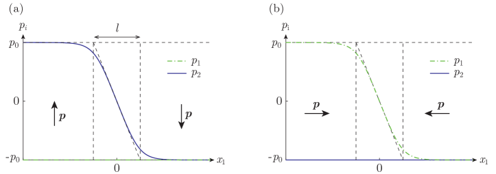
Figure 2: Polarization profiles of two 180^∘ domain walls: (a) charge-neutral wall, (b) charged wall. The profile in (a) corresponds to the solution (3.12) of (3.11) for $e=0$, and the profile in (b) is the solution of (3.23) under the equilibrium condition $d=0$.

This configuration is referred to as neutral 180^∘ domain wall due to the continuity of the normal component of $\bm{p}$ across the wall, which implies the absence of bound charges in the wall. In view of (3.5) and noting that the polarization profile is divergence-free, we can assume a uniform electric field $\bm{e}=e\tilde{\bm{e}}_{2}$ while satisfying Gauss’ law (2.5)₁.

We look for a traveling wave solution of the form

$$p_{1}(x_{1},t)=0,\quad p_{2}(x_{1},t)=p_{0}\check{p}_{2}(x_{1}-v_{180}t),$$ (3.10)

where $\xi=x_{1}-v_{180}t$ is the co-moving coordinate and $v_{180}$ the velocity of the wall. We denote by $\hat{\psi}_{180}(\overline{p}_{2})=\overline{\psi}_{s}(\overline{p}_{2}\tilde{\bm{e}}_{2})$ the section of the separation potential relevant for this situation. Inserting (3.10) into (3.7) yields an ordinary differential equation for $\check{p}_{2}(\xi)$:

$$\begin{aligned} \hat{C}_{g}p_{0}\check{p}_{2,\xi\xi}+\mu v_{180}p_{0}\check{p}_{2,\xi}-\frac{\hat{C}_{s}}{p_{0}}\hat{\psi}^{\prime}_{180}(\check{p}_{2})&=-e,\\ \hat{\psi}^{\prime}_{180}(\check{p}_{2}(\pm\infty))&=ep_{0}/\hat{C}_{s},\end{aligned}$$ (3.11)

where (3.11)₂ are the far-field boundary conditions at $\pm\infty$, and the prime denotes the derivative of a single-variable function with respect to its variable.

The equilibrium profile: $e=0$

In the absence of an electric field, (3.11) admits a static analytical solution with $v_{180}=0$ (Cao and Cross, 1991):

$$\check{p}_{2}^{\text{eq}}(\xi)=\frac{\sinh(\xi/\hat{\lambda}_{180})}{\sqrt{\hat{A}+\sinh^{2}(\xi/\hat{\lambda}_{180})}},\quad\mbox{with}\quad\hat{A}=\frac{3a_{4}+a_{2}}{2a_{4}+a_{2}}\quad\mbox{and}\quad\hat{\lambda}_{180}=p_{0}\sqrt{\frac{\hat{C}_{g}}{\hat{C}_{s}(6a_{4}+2a_{2})}}.$$ (3.12)

Based on this equilibrium profile, we relate $\hat{C}_{s}$ and $\hat{C}_{g}$ to the interface width and energy. We define the width $\hat{l}$ of the 180^∘ domain wall (see Figure 2) as

$$\hat{l}={2}/{\check{p}_{2,\xi}^{\text{eq}}(0)}$$ (3.13)

and its interfacial energy as

$$\hat{\Gamma}=\int_{-\infty}^{+\infty}\hat{\Psi}(\bm{e},\check{\bm{p}}^{\text{eq}},\nabla\check{\bm{p}}^{\text{eq}})\;\!\mathrm{d}\xi-\int_{-\infty}^{+\infty}W(\bm{e},\bm{p}^{\text{sharp}})\;\!\mathrm{d}\xi,$$ (3.14)

where

$$\bm{p}^{\text{sharp}}(\xi)=\begin{cases}+p_{0}\tilde{\bm{e}}_{2}\quad\mbox{for}\quad\xi<0,\\ -p_{0}\tilde{\bm{e}}_{2}\quad\mbox{for}\quad\xi\geq 0\end{cases}$$ (3.15)

is the sharp-interface solution of the 180^∘ domain wall. Noting that $\bm{e}$ is uniform and equal in both the phase-field and sharp-interface formulations and that the profile $\check{\bm{p}}^{\text{eq}}(\xi)$ is symmetric, (3.14) reduces to

$$\hat{\Gamma}=\int_{-\infty}^{+\infty}\left(\hat{C}_{s}\hat{\psi}_{s}(\check{\bm{p}}^{\text{eq}})+\frac{\hat{C}_{g}}{2}|\nabla\check{\bm{p}}^{\text{eq}}|^{2}\right)\;\!\mathrm{d}\xi=\int_{-\infty}^{+\infty}\left(\hat{C}_{s}\hat{\psi}_{180}\big{(}\check{p}_{2}^{\text{eq}}(\xi)\big{)}+\frac{\hat{C}_{g}p_{0}^{2}\check{p}_{2,\xi}^{\text{eq}}(\xi)^{2}}{2}\right)\;\!\mathrm{d}\xi.$$ (3.16)

The first integral of (3.11) in the equilibrium case ($e=0$, $v_{180}=0$), obtained by multiplying $\eqref{eq:ode1}$ by $\check{p}_{2,\xi}^{\text{eq}}$ and integrating from $\xi=-\infty$ to some arbitrary $\xi$, yields

$$2\hat{C}_{s}\hat{\psi}_{180}\big{(}\check{p}_{2}^{eq}(\xi)\big{)}={\hat{C}_{g}p_{0}^{2}\big{(}\check{p}_{2,\xi}^{eq}(\xi)\big{)}^{2}}.$$ (3.17)

From (3.17) we extract $\check{p}_{2,\xi}^{eq}(\xi)=\sqrt{2\hat{C}_{s}\hat{\psi}_{180}\big{(}\check{p}_{2}^{eq}(\xi)\big{)}/(\hat{C}_{g}p_{0}^{2})}$, which we exploit for the change of variable $\xi\rightarrow\overline{p}_{2}$ in (3.16). This yields

$$\hat{\Gamma}=\int_{-\infty}^{+\infty}2\hat{C}_{s}\hat{\psi}_{180}\big{(}\check{p}_{2}^{eq}(\xi)\big{)}\;\!\mathrm{d}\xi=\sqrt{2\hat{C}_{s}\hat{C}_{g}}p_{0}\hat{\eta},$$ (3.18)

where $\hat{\eta}=\int_{-1}^{1}\hat{\psi}_{180}(\overline{p})\;\!\mathrm{d}\overline{p}=\int_{-1}^{1}\sqrt{a_{0}+a_{1}\overline{p}^{2}+a_{2}\overline{p}^{4}+a_{4}\overline{p}^{6}}\;\!\mathrm{d}\overline{p}$ is a numerical coefficient. Further, combining (3.17) and (3.13) lets us express the width $\hat{l}$ as

$$\hat{l}=p_{0}\sqrt{{2\hat{C}_{g}}/{\hat{C}_{s}}}.$$ (3.19)

Conversely, (3.18) and (3.19) allows us to determine $\hat{C}_{g}$ and $\hat{C}_{s}$ from $\hat{\Gamma}$ and $\hat{l}$ via

$$\hat{C}_{g}=\frac{\hat{\Gamma}\hat{l}}{2\hat{\eta}p_{0}^{2}}\quad\mbox{and}\quad\hat{C}_{s}=\frac{\hat{\Gamma}}{\hat{\eta}\hat{l}}.$$ (3.20)

We note here that the interfacial energy $\hat{\Gamma}$ shall be taken as the physical interfacial energy $\gamma$ introduced in the sharp interface model, while $\hat{l}$ is viewed as a numerical parameter. Indeed, we take the perspective that the objective of the phase-field model is to properly account for the evolution of the pattern formed by domains or phases. In particular, the accuracy of the polarization profile within the diffuse interface (as compared to the physical profile) is of minor importance; instead, we aim to accurately capture the time evolution of the trace of domain walls. An accurate value of $\hat{\Gamma}$ to represent the interfacial energy is important to the extent that it is expected from the sharp interface model (see (2.9) and (2.19)) to affect the evolution of a curved interface. This latter point can be confirmed numerically. By contrast, $\hat{l}$ does not directly affect the evolution of the domain wall, but its choice results from a compromise between the following points:

• Because a diffuse interface needs sufficient numerical resolution (e.g., it should be discretized with typically no less than three points across its width in FFT-based schemes (Vidyasagar et al., 2017)), $\hat{l}$ cannot be taken too small.

• On the other hand, $\hat{l}$ cannot be taken too large either, because the characteristic electric field $\hat{e}_{c}=\hat{C}_{s}/p_{0}=\hat{\Gamma}/(\hat{\eta}\hat{l}p_{0})$ introduced in Section 3.1 must be sufficiently large for (3.9) to be satisfied with the physical electric field (notably to ensure that $\bm{p}$ remains close to one of the $\bm{p}_{\alpha}$ inside domains).

3.2.2 Equilibrium profile of a charged 180^∘ domain wall

The other characteristic 180^∘ domain wall is the so-called charged wall, in which the polarization is orthogonal to the domain wall (head-to-head or tail-to-tail). This configuration is usually not considered in the literature (see e.g. Cao and Cross, 1991; Schrade et al., 2013; Flaschel and De Lorenzis, 2020), because in the absence of free charges it is associated with high electric fields (of the order of $p_{0}/\epsilon$). As such, it implies high energies (see (3.1)) and is hence considered unstable in general. While it is true that ferroelectric domains evolve in such a way as to minimize the existence of charged 180^∘ domain walls, these cannot be completely disregarded. Indeed, charged portions of domain walls exist if one considers, e.g., two domains of antiparallel polarization separated by a closed boundary (see Figure 3).

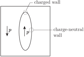
Figure 3: Sketch of an elliptical 180^∘ inclusion featuring both charge-neutral and charged domain walls.

This is the natural scenario of a newly nucleated domain in its parent domain.

Let us consider the 1D configuration of a charged 180^∘ domain wall with spontaneous polarization $\bm{p}(\bm{x},t)=p_{1}(x_{1},t)\tilde{\bm{e}}_{1}$ varying from the equilibrium close to $p_{0}\tilde{\bm{e}}_{1}$ at $x_{1}\rightarrow-\infty$ to the one near $-p_{0}\tilde{\bm{e}}_{1}$ at $x_{1}\rightarrow+\infty$ (see Figure 2(b)). We assume that the applied electric field is zero in the $\tilde{\bm{e}}_{2}$-direction, which implies, $\bm{e}(x_{1},t)=e_{1}(x_{1},t)\tilde{\bm{e}}_{1}$. As a result, the electric displacement is along the $\tilde{\bm{e}}_{1}$-direction and, because of (2.5)₁, it is uniform. Assuming further that it is time-independent, we write $\bm{d}(x_{1},t)=d\tilde{\bm{e}}_{1}$ where $d$ is constant. This allows us to write the non-zero electric field component as

$$e_{1}(x_{1},t)=\frac{d-p_{1}(x_{1},t)}{\epsilon}.$$ (3.21)

We look for a traveling wave solution of the form

$$p_{1}(x_{1},t)=p_{0}\check{p}_{1}(x_{1}-v_{180}^{c}t),$$ (3.22)

where $\xi=x_{1}-v_{180}^{c}t$ is the co-moving coordinate, $v_{180}^{c}$ the velocity of the charged wall, and $\check{p}_{1}(\xi)$ is a smooth, differentiable function. Inserting (3.22) into (3.7) and resorting to (3.21) yields the ordinary differential equation for $\check{p}_{1}(\xi)$,

$$\begin{aligned} \hat{C}_{g}p_{0}\check{p}_{1,\xi\xi}+\mu v_{180}^{c}p_{0}\check{p}_{1,\xi}-\frac{\hat{C}_{s}}{p_{0}}{\hat{\psi}^{c}_{180}}^{\prime}(\check{p}_{1})&=-\frac{d}{\epsilon},\\ {\hat{\psi}^{c}_{180}}^{\prime}\big{(}\check{p}_{1}(\pm\infty)\big{)}&=\frac{p_{0}d}{\epsilon\hat{C}_{s}},\end{aligned}$$ (3.23)

where we have introduced the effective double well potential $\hat{\psi}_{180}^{c}$ for charged walls as

$$\hat{\psi}_{180}^{c}(\overline{p})=\hat{\psi}_{180}(\overline{p})+\frac{p_{0}^{2}}{2\epsilon\hat{C}_{s}}\overline{p}^{2}=\hat{\psi}_{180}(\overline{p})+\frac{\hat{\eta}\hat{l}p_{0}^{2}}{2\epsilon\hat{\Gamma}}\overline{p}^{2}$$ (3.24)

with $\hat{\psi}_{180}(\overline{p})$ the cut of $\overline{\psi}_{s}(\overline{\bm{p}})$ defined in Section 3.2.1.

The equilibrium profile: $d=0$

In the absence of an electric displacement, (3.23) admits a static solution with $v_{180}^{c}=0$. In this case, (3.23) differs from (3.11) only through the effective double-well potential $\hat{\psi}_{180}^{c}$, which replaces $\hat{\psi}_{180}$. The fact that, physically, the values of $\check{p}_{1}$ at infinity given by (3.23)₂ shall remain close to 1 requires that $\hat{\psi}_{180}^{c}$ differs little from $\hat{\psi}_{180}$, i.e.,

$$\hat{\zeta}=\frac{\hat{\eta}\hat{l}p_{0}^{2}}{\epsilon\hat{\Gamma}}\ll 1.$$ (3.25)

Equation (3.25) can be seen as an upper bound on $\hat{l}$, and it is nothing but condition (3.9) with $\left|\bm{e}\right|\sim p_{0}/\epsilon$, which corresponds to the typical electric field that develops in charged domain walls.

One can show that under the assumption (3.25) the width and interfacial energy of a charged 180^∘ domain wall are approximately equal to those of the corresponding neutral walls given by (3.18) and (3.19), respectively. In other words, width and interfacial energy of a 180^∘ domain wall are essentially independent of the relative orientation of the wall and the polarization directions.

3.2.3 Velocity of 180^∘ domain walls

We proceed to consider the steady-state velocity of 180^∘ domain walls, beginning with neutral ones and later concluding the solution for charged ones. Taking the first integral of (3.11)₁, we express the velocity $v_{180}$ of the domain wall as

$$v_{180}=\frac{\hat{C}_{s}\big{[}\hat{\psi}_{180}\big{(}\check{p}_{2}(+\infty)\big{)}-\hat{\psi}_{180}\big{(}\check{p}_{2}(-\infty)\big{)}\big{]}-e\big{[}\check{p}_{2}(+\infty)-\check{p}_{2}(-\infty)\big{]}}{\mu p_{0}\int_{-\infty}^{+\infty}(\check{p}_{2,\xi})^{2}\;\!\mathrm{d}\xi},$$ (3.26)

which involves the unknown function $\check{p}_{2}(\xi)$. Under the assumption that (3.9) is satisfied, the traveling wave problem (3.11) with $e\neq 0$ is a perturbation of the case $e=0$. Hence, to first order in $e/\hat{e}_{c}$ the velocity (3.26) can be approximated using the equilibrium profile $\check{p}_{2}^{eq}$, which yields

$$v_{180}\approx\frac{2e}{\mu p_{0}\int_{-\infty}^{+\infty}(\check{p}_{2,\xi}^{eq})^{2}\;\!\mathrm{d}\xi}=\hat{c}_{180}f_{180},$$ (3.27)

where $\hat{c}_{180}=\hat{l}/(2\hat{\eta}\mu p_{0}^{2})$ is a kinetic coefficient, and $f_{180}=2ep_{0}$ denotes the value of the driving traction (2.22) for a straight, neutral 180^∘ domain wall. (In deriving (3.27), we used (3.17) and performed the same change of variable in the integral as in (3.18).) For charged domain walls, the driving traction (2.22) reads $f_{180}^{c}=2p_{0}d/\epsilon$. One can show that, under the assumption (3.25), the linear kinetic relation (3.27) holds for charged domain walls as well, where it reads $v_{180}^{c}\approx\hat{c}_{180}f_{180}^{c}$. We point out that the above analysis, of course, presumes that stable motion of a domain wall at constant speed is feasible. While this is realistic for neutral 180^∘ domain walls, the high energy associated with their charged counterparts precludes their stable motion over significant times in general.

3.2.4 Equilibrium profile of a neutral 90^∘ domain wall

For studying 90^∘ domain walls, the basis of spontaneous polarizations $\{\bm{p}_{\alpha}\}_{\alpha\in(1,6)}$ defined in (2.13) and the multi-well potential (3.2) are rotated by $+\pi/4$ around the direction $\tilde{\bm{e}}_{3}$. We consider a 1D head-to-tail 90^∘ domain wall with spontaneous polarization $\bm{p}(\bm{x},t)=p_{2}(x_{1},t)\tilde{\bm{e}}_{2}+p_{1}(x_{1},t)\tilde{\bm{e}}_{1}$, varying from the equilibrium close to $p_{0}(\tilde{\bm{e}}_{1}+\tilde{\bm{e}}_{2})/\sqrt{2}$ at $x_{1}\rightarrow-\infty$ to the one near $p_{0}(\tilde{\bm{e}}_{1}-\tilde{\bm{e}}_{2})/\sqrt{2}$ at $x_{1}\rightarrow+\infty$ (see Figure 4(a)).

Figure 4: Polarization profiles of two 90^∘ domain walls: (a) charge-neutral wall, (b) charged wall. The profile in (a) corresponds to the solution of (3.28) for $e=0$, while that in (b) is for the equilibrium condition $d=0$.

When looking for an equilibrium or a traveling wave solution of (3.7), the $p_{1}$-component appears to vary across the domain wall. As a result, for Gauss’ law (2.5)₁ to be satisfied, the electric field is non-uniform and the polarization profile does not admit an analytical solution.

Therefore, we compute an approximation of the 90^∘ domain wall profile, by assuming that $p_{1}=p_{0}/\sqrt{2}$ remains constant across the interface. This assumption is all the more valid as the 90^∘ barrier in $\overline{\psi}_{s}$ is located along the straight line connecting two orthogonal polarization states, i.e., $\hat{\chi}=0.5$ in (3.4). As mentioned in Section 3.2.1, in the phase-field formulation we do not aim for an accurate representation of the polarization profile across domain walls, which justifies considering $\hat{\chi}$ as a numerical parameter that may be freely chosen. Under this assumption, we suppose that we apply a uniform electric field $\bm{e}=e\tilde{\bm{e}}_{2}$ while satisfying Gauss’ law (2.5)₁. Akin to the 180^∘ domain wall (cf. (3.10)), we seek a traveling wave solution $p_{2}(x_{1},t)$. Inserting (3.10)₂ in (3.7), where $\hat{\psi}_{s}$ has been properly rotated, yields the following ordinary differential equation for $\check{p}_{2}(\xi)$:

$$\begin{aligned} \hat{C}_{g}p_{0}\check{p}_{2,\xi\xi}+\mu v_{90}p_{0}\check{p}_{2,\xi}-\frac{\hat{C}_{s}}{p_{0}}\hat{\psi}^{\prime}_{90}(\check{p}_{2})&=-e,\\ \hat{\psi}^{\prime}_{90}\big{(}\check{p}_{2}(\pm\infty)\big{)}&=ep_{0}/\hat{C}_{s},\end{aligned}$$ (3.28)

where $v_{90}$ denotes the corresponding velocity. The only difference to (3.11) lies in the section $\hat{\psi}_{90}(\overline{p}_{2})$ of $\overline{\psi}_{s}(\overline{\bm{p}})$, given by

$$\hat{\psi}_{90}(\overline{p}_{2})=\overline{\psi}_{s}\left(\frac{1/\sqrt{2}-\overline{p}_{2}}{\sqrt{2}},\frac{1/\sqrt{2}+\overline{p}_{2}}{\sqrt{2}},0\right)=a^{\ast}_{0}+a^{\ast}_{1}\overline{p}_{2}^{2}+a^{\ast}_{2}\overline{p}_{2}^{4}+a^{\ast}_{4}\overline{p}_{2}^{6},$$ (3.29)

where

$$\begin{aligned} a^{\ast}_{0}&=a_{0}+a_{1}/2+a_{2}/8+a_{3}/16+a_{4}/32,\qquad a^{\ast}_{1}=a_{1}+3a_{2}/2-a_{3}/4+30a_{4}/32,\\ a^{\ast}_{2}&=a_{2}/2+a_{3}/4+60a_{4}/32,\qquad\mbox{and}\quad a^{\ast}_{4}=a_{4}/4.\end{aligned}$$ (3.30)

Here and in the following, superscript ^∗ indicates quantities associated with 90^∘ domain walls.

The equilibrium profile: $e=0$

For $e=0$, (3.28) admits an analytical solution $\check{p}_{2}^{\text{eq}\ast}(\xi)$ similar to (3.12). Noting that $\check{p}_{2}^{\text{eq}\ast}(\xi)$ varies from $-1/\sqrt{2}$ at $\xi\rightarrow-\infty$ to $1/\sqrt{2}$ at $\xi\rightarrow\infty$, we define the width of the 90^∘ domain wall as

$$\hat{l}_{90}=\frac{\sqrt{2}}{\check{p}_{2}^{\text{eq}\ast}(0)}.$$ (3.31)

The interfacial energy $\hat{\Gamma}_{90}$ has the same definition as (3.14), where now $\check{\bm{p}}^{\text{eq}}$ and $\bm{p}^{\text{sharp}}$ are replaced by the phase-field and sharp-interface profiles of the 90^∘ domain wall, respectively. The derivation (3.16)-(3.18) holds with $\hat{\psi}_{90}(\overline{p}_{2})$ in place of $\hat{\psi}_{180}(\overline{p}_{2})$, and we obtain

$$\hat{\Gamma}_{90}=\frac{\hat{\eta}^{*}}{\hat{\eta}}\hat{\Gamma},$$ (3.32)

with $\hat{\eta}^{*}=\int_{-1/\sqrt{2}}^{1/\sqrt{2}}\hat{\psi}_{90}(\overline{p}_{2})\;\!\mathrm{d}\overline{p}=\int_{-1/\sqrt{2}}^{1/\sqrt{2}}\sqrt{a_{0}^{*}+a_{1}^{*}\overline{p}^{2}+a_{2}^{*}\overline{p}^{4}+a_{4}^{*}\overline{p}^{6}}\;\!\mathrm{d}\overline{p}$. In addition, re-writing (3.17) for the 90^∘ domain wall lets us compute $\check{p}_{2,\xi}^{\text{eq}\ast}(\xi)$ and derive

$$\hat{l}_{90}=\frac{\hat{l}}{\sqrt{2\hat{h}_{90}}}.$$ (3.33)

3.2.5 Equilibrium profile of a charged 90^∘ domain wall

The charged 90^∘ domain wall corresponds to the head-to-head (or tail-to-tail) configuration (see Figure 4(b)). The transition from neutral to charged 90^∘ domain walls is in all points equivalent to the transition from neutral to charged 180^∘ domain walls. To summarize the main point, for charged 90^∘ domain walls an effective potential

$$\hat{\psi}_{90}^{c}(p_{1})=\hat{\psi}_{90}(p_{1})+\frac{\hat{\eta}\hat{l}p_{0}^{2}}{2\epsilon\hat{\Gamma}}p_{1}^{2}$$ (3.34)

appears in the traveling wave solution (as in (3.23)). Likewise, the width and interfacial energy of the charged 90^∘ -domain wall are approximately equal to those of the neutral wall under condition (3.25).

3.2.6 Velocity of 90^∘ domain walls

Following the same procedure as for 180^∘ domain walls, the first integral of (3.28) allows us to write $v_{90}$ as an expression analogous to (3.26), where one substitutes $\hat{\psi}_{90}$ for $\hat{\psi}_{180}$. In the regime $e\ll\hat{e}_{c}$, $\check{p}_{2}$ can be approximated by the equilibrium profile of (3.28), which yields

$$v_{90}\approx\frac{\sqrt{2}e}{\mu p_{0}\int_{-\infty}^{+\infty}(\check{p}_{2,\xi}^{\text{eq}*})^{2}\;\!\mathrm{d}\xi}=\hat{c}_{90}f_{90},$$ (3.35)

where $\hat{c}_{90}=\hat{l}/(2\hat{\eta}^{*}\mu p_{0}^{2})$ and $f_{90}=\sqrt{2}ep_{0}$ denote, respectively, the kinetic coefficient and driving traction associated with the 90^∘ domain wall. Under the condition (3.25), the charged 90^∘ domain wall shows the same linear kinetics, with coefficient $\hat{c}_{90}$, as its neutral counterpart.

3.3 Summary of the properties of 180^∘ and 90^∘ domain walls

Interface energy and width

We have computed exactly the interfacial energy $\hat{\Gamma}$ and width $\hat{l}$ of a neutral 180^∘ domain wall and found that these can be arbitrarily prescribed by choosing $\hat{C}_{g}$ and $\hat{C}_{s}$ according to (3.20). While we expect to use the physical domain wall energy for $\hat{\Gamma}$, $\hat{l}$ is viewed as a numerical parameter to be chosen in light of considerations discussed above (the more stringent condition on $\hat{l}$ being (3.25)). The charged 180^∘ domain wall has approximately the same equilibrium properties as the neutral one, as long as (3.25) is satisfied.

For the classical head-to-tail 90^∘ domain wall, we have derived an approximation of its interfacial energy $\hat{\Gamma}_{90}$ and width $\hat{l}_{90}$, whose accuracy is best for $\hat{\chi}=0.5$. The ratio $\hat{\Gamma}_{90}/\hat{\Gamma}$ can be set according to its physical value by independently setting $\hat{h}_{90}$. Indeed, (3.32) indicates that this ratio is equal to that of the integrals over the 90^∘ and 180^∘ barriers in the multi-well potential $\overline{\psi}_{s}(\overline{\bm{p}})$. Finally, the width $\hat{l}_{90}$ is automatically determined by (3.33) and cannot be set independently. Note that, because we view $\hat{l}_{90}$ as a numerical regularization length, there is no need to prescribe it independently. However, where it is viewed as the physical width of a 90^∘ domain wall, the phase-field framework can be modified such that $\hat{l}_{90}$ is chosen in agreement with its physical value (Flaschel and De Lorenzis, 2020).

Kinetics

We have found that, in the regime $\left|\bm{e}\right|\ll\hat{e}_{c}$, the Allen–Cahn evolution equation (3.6) implies approximately a linear kinetic relation between the velocity of domain walls and the driving traction. In addition, the 180^∘ and 90^∘ domain walls have different kinetic coefficients related by the ratio $\hat{\eta}^{*}/\hat{\eta}$. Whereas the choice of inverse mobility $\mu$ allows us to independently set one kinetic coefficient, the second one is automatically determined by the ratio of interfacial energies (see (3.32) and (3.35)).

This linear kinetics is not representative of the complex nonlinear kinetics of domain walls, which experiments and atomic-scale modeling discussed in Section 2.2 show. Yet, a proper account of the kinetics of domain walls is important in two respects. First, different kinetics yield different microstructure evolution, hence a proper account of the kinetics is needed for obtaining an accurate description of switching at the mesoscale. Second and more importantly, rate-dependent effects in the macroscopic footprints of polarization switching—such as those discussed in Section 1—are a direct consequence of the kinetics of domain walls. Having a phase-field model that permits domain wall motion with nonlinear kinetics requires us to revise the evolution equation (3.6). This is the subject of the general kinetics model introduced in Section 4.

4 General kinetics model

In this section, we introduce a new phase-field model for ferroelectrics, which regularizes the sharp-interface model of Section 2 while conserving nonlinear and independent kinetics for 180^∘ and 90^∘ domain walls. We first formulate the model in Section 4.1, before computing analytical traveling wave solutions for 180^∘ and 90^∘ domain walls in Section 4.2. The main properties of straight domain walls are summarized and compared to those of the Allen–Cahn model in Section 4.3. A numerical implementation of the present model will be performed in Part II, which must also account for the special behavior of curved domain walls and triple and quadruple points at which multiple phases meet.

4.1 Model formulation

A regularized electric enthalpy

In the general kinetics model, we use a multi-phase field $\bm{\varphi}(\bm{x},t)\in(0,1)^{N}$, where $N$ is the number of domains, and for tetragonal ferroelectrics we use $N=6$. Let $\varphi_{\alpha}$ denote the volume fraction of domain $\alpha$, so that the spontaneous polarization is defined as

$$\bm{p}(\bm{x},t)=\tilde{\bm{p}}\big{(}\bm{\varphi}(\bm{x},t)\big{)}=\sum_{\alpha=1}^{6}\varphi_{\alpha}(\bm{x},t)\bm{p}_{\alpha}.$$ (4.1)

We introduce the electric enthalpy ${\Psi}$, which regularizes $W(\bm{e},\bm{p})$, as

$$\Psi(\bm{e},\bm{\varphi},\nabla\bm{\varphi})=\underbrace{-\frac{\epsilon}{2}\bm{e}\cdot\bm{e}-\Big{(}\sum_{\alpha=1}^{6}\varphi_{\alpha}\bm{p}_{\alpha}\Big{)}\cdot\bm{e}}_{W(\bm{e},\tilde{\bm{p}}(\bm{\varphi}))}\,+\,C_{s}\psi_{s}(\bm{\varphi})+p_{0}^{2}C_{g}\sum_{\alpha=1}^{6}|\nabla\varphi_{\alpha}|^{2},$$ (4.2)

where $C_{s}$ and $C_{g}$ are two positive constants, and $\psi_{s}$ is a multi-well potential with minima at (or in the neighborhood of) the six values of $\bm{\varphi}$ associated with the spontaneous polarization states: $\bm{\varphi}=(1,0,\ldots,0)$ and its permutations. There exists several possibilities for the choice of $\psi_{s}$, and the optimal one depends on the values of the physical parameters. Here, we discuss two simple forms for $\psi_{s}$ that admit analytical insight, even though the framework is sufficiently general to allow for other choices as well. For analytical derivations, we introduce

$$\psi_{s}^{(n)}(\bm{\varphi})=\omega^{(n)}(\bm{\varphi})+\tau(\bm{\varphi}),$$ (4.3)

with

$$\begin{aligned} \omega^{(n)}(\bm{\varphi})&=4^{n}\Bigg{(}\sum_{\{\alpha,\beta\}\in\mathcal{I}_{180}}\left|\varphi_{\alpha}\right|^{n}\left|\varphi_{\beta}\right|^{n}+h_{90}\sum_{\{\alpha,\beta\}\in\mathcal{I}_{90}}\left|\varphi_{\alpha}\right|^{n}\left|\varphi_{\beta}\right|^{n}\Bigg{)},\\ \tau(\bm{\varphi})&=C_{t}\sum_{\{\alpha,\beta,\gamma\}\in\mathcal{T}}\left|\varphi_{\alpha}\right|\left|\varphi_{\beta}\right|\left|\varphi_{\gamma}\right|,\end{aligned}$$ (4.4)

where $h_{90}$ denotes the height of the 90^∘ barrier relative to the 180^∘ barrier, $C_{t}>0$ is a numerical parameter and $\mathcal{T}=\{(\alpha,\beta,\gamma):\alpha,\beta,\gamma\in\mathcal{D},\alpha\neq\beta\neq\gamma\}$, and we consider $n=1$ and $n=2$.

As we shall see below, $\psi_{s}^{(1)}$ has the advantage that the effective potential for charged walls has minima that remain at the spontaneous polarization states but the drawback of presenting discontinuities in its derivatives. On the other hand, with $\psi_{s}^{(2)}$ discontinuities in the derivatives are absent, but the zeros and minima of the effective potential for charged walls are shifted from the spontaneous polarization states.

The contribution $\tau(\bm{\varphi})$ to $\psi_{s}^{(n)}(\bm{\varphi})$ serves to avoid the spurious appearance of a third phase in a domain wall by penalizing the simultaneous occurrence of more than two phases. Despite the apparently complicated expression of $\psi_{s}^{(n)}$, its section $\psi_{180}(\varphi)=\psi_{s}^{(n)}\big{(}(\varphi,1-\varphi,0,0,0,0)\big{)}$ associated with a 180^∘ domain wall reduces to

$$\psi_{180}(\varphi)=4^{n}\left|\varphi\right|^{n}\left|1-\varphi\right|^{n},$$ (4.5)

which is a double-obstacle ($n=1$) or double-well ($n=2$) potential of unitary barrier. Similarly, the section $\psi_{90}(\varphi)=\psi_{s}^{(n)}\big{(}(\varphi,0,1-\varphi,0,0,0)\big{)}$ associated with a 90^∘ domain wall reads

$$\psi_{90}(\varphi)=4^{n}h_{90}\left|\varphi\right|^{n}\left|1-\varphi\right|^{n}.$$ (4.6)

Governing equations

Whereas Gauss’ law (2.5)₁ and Faraday’s equation (2.6)₁ apply without change, the main difference between our general kinetics model and the classical phase-field model resides in the evolution equation for the multi-phase field, which we define as

$$\dot{\varphi}_{\alpha}=\sum_{\beta=1}^{6}\sqrt{\left|\nabla\varphi_{\alpha}\cdot\nabla\varphi_{\beta}\right|}\,G_{\beta\alpha}(h_{\beta\to\alpha})\quad\mbox{for}\quad\alpha=1\ldots 6,$$ (4.7)

where $G_{\alpha\beta}=G_{\beta\alpha}:\mathbb{R}\rightarrow\mathbb{R}$ is the kinetic function associated with the transformation between phases $\alpha$ and $\beta$, and $h_{\beta\to\alpha}$ denotes the relative variational derivative of ${\Psi}$,

$$h_{\beta\to\alpha}\left(\bm{e},\bm{\varphi},\nabla^{2}\bm{\varphi}\right)=-\frac{\delta\Psi}{\delta\varphi_{\alpha}}+\frac{\delta\Psi}{\delta\varphi_{\beta}}=-\frac{\partial\Psi}{\partial\varphi_{\alpha}}+\frac{\partial\Psi}{\partial\varphi_{\beta}}+\operatorname{div}\left(\frac{\partial\Psi}{\partial\nabla\varphi_{\alpha}}-\frac{\partial\Psi}{\partial\nabla\varphi_{\beta}}\right).$$ (4.8)

Inserting (4.2) in (4.8) yields

$$h_{\beta\to\alpha}\left(\bm{e},\bm{\varphi},\nabla^{2}\bm{\varphi}\right)=\bm{e}\cdot(\bm{p}_{\alpha}-\bm{p}_{\beta})-C_{s}\bigg{(}\frac{\partial\psi_{s}}{\partial\varphi_{\alpha}}-\frac{\partial\psi_{s}}{\partial\varphi_{\beta}}\bigg{)}+2p_{0}^{2}C_{g}\big{(}\nabla^{2}\varphi_{\alpha}-\nabla^{2}\varphi_{\beta}\big{)}.$$ (4.9)

For tetragonal ferroelectrics, we distinguish between two types of transformations: the motion of 180^∘ and 90^∘ domain walls. Hence, we take the function $G_{\alpha\beta}$ as $G_{180}$ for $\{\alpha,\beta\}\in\mathcal{I}_{180}$ and $G_{90}$ for $\{\alpha,\beta\}\in\mathcal{I}_{90}$. By the second law of thermodynamics, $G_{180}$ and $G_{90}$ must be odd functions that satisfy the constraints

$$G_{180}(h)h\geq 0\quad\mbox{and}\quad G_{90}(h)h\geq 0\quad\mbox{for all}\;h\in\mathbb{R}.$$ (4.10)

Indeed, as we will show in Section 4.2, these two functions specify the kinetic relations of 180^∘ and 90^∘ domain walls in the sense of (2.11) in the sharp-interface model. Condition (4.10), like (2.12), ensures the positivity of the dissipation in the phase-field model.

Equation (4.7) is used with an initial condition $\bm{\varphi}(\bm{x},0)$ that satisfies

$$\sum_{\alpha=1}^{6}\varphi_{\alpha}(\bm{x},0)=1\quad\mbox{for all}\quad\bm{x}\in\Omega.$$ (4.11)

Using that $G_{180}$ and $G_{90}$ are odd functions, one can show that (4.7) guarantees $\sum_{\alpha=1}^{6}\dot{\varphi}_{\alpha}=0$, whereby (4.11) holds for all times if it holds for the initial condition.

Comparison with other phase-field models with nonlinear kinetics

The evolution equation (4.7) is an extension to multiple phases of the hybrid model introduced by Alber and Zhu (2013) in the setting of stress-driven phase transformations between two phases. In particular, in a domain wall between two phases, say $\alpha=1$ and $\beta=2$, for which $\varphi_{2}(\bm{x},0)=1-\varphi_{1}(\bm{x},0)$ and $\varphi_{\gamma}(\bm{x},0)=0$ for $\gamma=3\ldots 6$, (4.7) reduces to

$$\begin{aligned} \dot{\varphi}_{1}&=\left|\nabla\varphi_{1}\right|G_{180}\left(h_{2\to 1}\right),\quad\varphi_{2}=1-\varphi_{1},\\ \varphi_{\gamma}&=0\quad\mbox{for}\quad\gamma=3\ldots 6.\end{aligned}$$ (4.12)

(4.12)₁ is akin to Equation (1.3) of Alber and Zhu (2013) (there formulated in the context of stress-driven transformations). Note that the double-well potential proposed by Alber and Zhu (2013) is a variation of (4.5).

Similarly, (4.12)₁ is reminiscent of the evolution equation (2.7) of Agrawal and Dayal (2015a), which derives from a conservation law for the number of interfaces. However, in their work, the free-energy density was regularized differently from ours and that of Alber and Zhu (2013), without resort to a double-well potential but through a regularized Heaviside function. Further, Agrawal and Dayal (2015a) included a source term in the evolution equation for $\varphi$ to account for the nucleation of new domains. In our case, in the absence of such a source term, (4.7) only propagates domain walls, while for nucleation new domains shall be introduced explicitly according to an appropriate criterion, which we do not discuss here.

4.2 Analytical solutions for 180^∘ and 90^∘ domain walls

In this section, we compute analytical traveling wave solutions for the propagation of straight 180^∘ and 90^∘ domain walls as obtained from the general kinetics model. In doing so, we follow in one dimension a procedure outlined, e.g., in Fried and Gurtin (1994) for Allen–Cahn-type models. In particular, we demonstrate the nonlinear kinetics of domain walls that the general kinetics model permits, and we compare our findings to the Allen–Cahn model.

4.2.1 Neutral 180^∘ domain wall profile and kinetics

We consider a straight 180^∘ domain wall with polarization $\bm{p}(x_{1},t)=p_{2}(x_{1},t)\tilde{\bm{e}}_{2}$, separating the spontaneous polarizations $\bm{p}_{3}=p_{0}\tilde{\bm{e}}_{2}$ at $x_{1}\rightarrow-\infty$ and $\bm{p}_{4}=-p_{0}\tilde{\bm{e}}_{2}$ at $x_{1}\rightarrow+\infty$ (see Figure 5(b)).

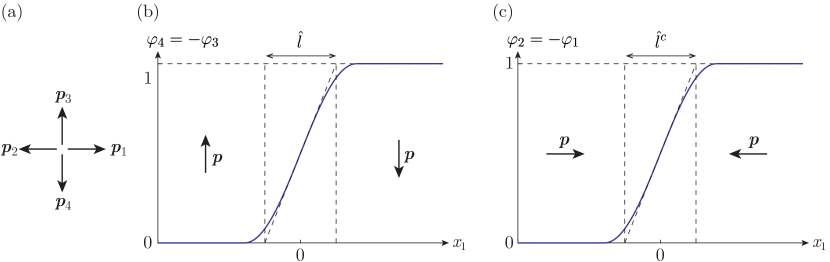
Figure 5: (a) Basis of spontaneous polarization states. Phase-field profiles of two 180^∘ domain walls: (b) charge-neutral wall, (c) charged wall. The profile in (b) corresponds to (4.26) with $\varphi=\varphi_{4}$ and that in (c) to the solution of (4.34) with $\varphi=\varphi_{2}$.

The phase fields not related to the two phases under consideration, i.e., $\varphi_{\gamma}$ for $\gamma\in\{1,2,5,6\}$ are initially assumed identically zero and, in view of (4.7), remain zero for all time. Hence, only the phase fields $\varphi_{3}$ and $\varphi_{4}$, satisfying $\varphi_{3}+\varphi_{4}=1$, are non-trivial. To simplify notation, we define $\varphi=\varphi_{4}$ to write the polarization profile as

$$\bm{p}_{180}(\varphi)=p_{0}(1-2\varphi)\tilde{\bm{e}}_{2}.$$ (4.13)

As in Section 3.2.1, we can assume a uniform electric field $\bm{e}=e\tilde{\bm{e}}_{2}$ while satisfying Gauss’ law (2.5)₁. The evolution equations (4.7) for $\varphi_{3}$ and $\varphi_{4}$ are identical and are written as an equation for $\varphi$:

$$\dot{\varphi}=\left|\varphi_{,x_{1}}\right|G_{180}\big{(}h_{3\rightarrow 4}(\varphi,\varphi_{,x_{1}x_{1}})\big{)},$$ (4.14)

where the driving force (4.9) reads

$$h_{3\rightarrow 4}(\varphi,\varphi_{,x_{1}x_{1}})=-2p_{0}e-C_{s}\psi^{\prime}_{180}(\varphi)+4C_{g}p_{0}^{2}\varphi_{,x_{1}x_{1}}.$$ (4.15)

As in Section 3.2, we seek a traveling wave solution of (4.14) of the form

$$\varphi(x_{1},t)=\check{\varphi}(x_{1}-v_{180}t)$$ (4.16)

and introduce $\xi=x_{1}-v_{180}t$. Inserting (4.16) into (4.14) yields

$$-v_{180}\check{\varphi}_{,\xi}=\left|\check{\varphi}_{,\xi}\right|G_{180}\big{(}h_{3\rightarrow 4}(\check{\varphi},\check{\varphi}_{,\xi\xi})\big{)}.$$ (4.17)

Without loss of generality, assuming that the solution satisfies $\check{\varphi}_{,\xi}\geq 0$ for all $\xi$, (4.17) simplifies to

$$\begin{aligned} &v_{180}=G_{180}\bigg{(}2p_{0}e+{C_{s}}\psi^{\prime}_{180}(\check{\varphi})-4C_{g}p_{0}^{2}\check{\varphi}_{,\xi\xi}\bigg{)},\\ &\check{\varphi}(-\infty)=0,\quad\check{\varphi}(+\infty)=1,\quad\check{\varphi}_{,\xi}(\pm\infty)=0,\end{aligned}$$ (4.18)

where we have appended in (4.18)_2,3,4 the far-field boundary conditions on $\check{\varphi}$ consistent with the polarization states assumed at infinity. Note that (4.18)_2,3,4 are in fact two boundary conditions, since the vanishing spatial derivative of $\check{\varphi}$ at infinity is inherited from the former two conditions (4.18)_2,3. For a given applied electric field $e$, (4.18) can be solved for $\big{(}v_{180},\check{\varphi}(\xi)\big{)}$. We assume here that $G_{180}$ is monotonous on $\mathbb{R}$ and hence invertible, and we write its inverse as $G_{180}^{-1}$. Hence, (4.18)₁ is rewritten as

$$2p_{0}e+{C_{s}}\psi^{\prime}_{180}(\check{\varphi})-4C_{g}p_{0}^{2}\check{\varphi}_{,\xi\xi}=G_{180}^{-1}(v_{180}).$$ (4.19)

We compute the first integral of (4.19) by multiplying by $\check{\varphi}_{,\xi}$ and integrating with the condition at $-\infty$, which yields:

$$\big{[}2p_{0}e-G_{180}^{-1}(v_{180})\big{]}\check{\varphi}+C_{s}\psi_{180}(\check{\varphi})-2C_{g}p_{0}^{2}(\check{\varphi}_{,\xi})^{2}=0,$$ (4.20)

where we have used the fact that $\psi_{180}(0)=0$. Further prescribing condition (4.18)_3,4 at $+\infty$ and noting that $\psi_{180}(1)=0$, requires that

$$2p_{0}e=G_{180}^{-1}(v_{180})\quad\Rightarrow\quad v_{180}=G_{180}(2p_{0}e),$$ (4.21)

and (4.20) reduces to an equation for $\check{\varphi}(\xi)$ only:

$$C_{s}\psi_{180}(\check{\varphi})-2C_{g}p_{0}^{2}(\check{\varphi}_{,\xi})^{2}=0.$$ (4.22)

Equation (4.22) is similar to (3.17) in the Allen–Cahn model. However, note that (4.22) holds for all $e$. Therefore, the profile is the same at equilibrium ($e=0$) and with an applied external electric field ($e\neq 0$). In particular, the polarization inside domains remains exactly equal to the spontaneous polarizations even under non-zero electric fields. This is in contrast to the Allen–Cahn model, whose equilibrium polarization profile is given by (3.17). That equation, however, only provides an approximation of the profile in the presence of an electric field, which is valid only under condition (3.9).

Adopting definitions for the interfacial energy,

$$\Gamma=\int_{-\infty}^{+\infty}\Psi(\bm{e},\check{\bm{\varphi}},\nabla\check{\bm{\varphi}})\;\!\mathrm{d}\xi-\int_{-\infty}^{+\infty}W(\bm{e},\bm{p}^{\text{sharp}})\;\!\mathrm{d}\xi,$$ (4.23)

and the interfacial width,

$$l=1/\check{\varphi}_{,\xi}(0),$$ (4.24)

equivalent to those of Section 3.2, one can show using (4.22) that these quantities are given by expressions analogous to (3.18) and (3.19), namely,

$$\Gamma=\eta p_{0}\sqrt{2C_{s}C_{g}}\quad\mbox{and}\quad l=p_{0}\sqrt{2C_{g}/C_{s}},$$ (4.25)

with $\eta=2\int_{0}^{1}\sqrt{\psi_{180}(\varphi)}\;\!\mathrm{d}\varphi$. In particular, with $\psi_{180}$ given by (4.5) we obtain $\eta=\pi/2$ for $n=1$ and $\eta=4/3$ for $n=2$.

By setting the origin to $\check{\varphi}(0)=1/2$, (4.22) forms an initial value problem for $\check{\varphi}(\xi)$, starting at $\xi=0$ and to be solved for both increasing and decreasing $\xi$. Its integration yields

$$\check{\varphi}(\xi)=\begin{cases}0&\quad\mbox{for}\;\xi<-{\pi l}/{4},\\ \cos^{2}\left(\displaystyle\frac{\pi}{4}-\frac{\xi}{l}\right)&\quad\mbox{for}\;-{\pi l}/{4}\leq\xi\leq{\pi l}/{4},\\ 1&\quad\mbox{for}\;\xi>{\pi l}/{4},\end{cases}$$ (4.26)

when using $\psi_{s}^{(1)}$ and

$$\check{\varphi}(\xi)=\frac{\mathrm{e}^{4\xi/l}}{1+\mathrm{e}^{4\xi/l}},$$ (4.27)

for $\psi_{s}^{(2)}$. Note that with $\psi_{s}^{(1)}$ the diffuse interface representing the domain wall is localized in the interval $(-\pi l/4,\pi l/4)$.

With regards to kinetics, in (4.21)₂ $2p_{0}e=f$ corresponds to the driving traction (2.22) of the straight, neutral 180^∘ domain wall in the sharp-interface model. Hence, $G_{180}$ directly provides the kinetic relation for 180^∘ domain walls (i.e., (2.11) in the sharp-interface model). Therefore, the general kinetic model allows us to choose the kinetic relation arbitrarily (in the set of monotonously increasing odd functions that satisfy (4.10)). In particular, for modeling ferroelectrics, a physics-based choice for $G_{180}$ is to adopt the functional form (2.19) derived from experiments. In addition, note that for the neutral 180^∘ domain wall, the kinetic relation is exactly given by (4.21)₂ for all $e$, whereas with the Allen–Cahn model the linear kinetic relation (3.27) is only an approximation valid under the condition (3.9).

4.2.2 Charged 180^∘ domain wall profile and kinetics

We consider the same charged domain wall as in Section 3.2.2, i.e., $\bm{p}(x_{1},t)=p_{1}(x_{1},t)\tilde{\bm{e}}_{1}$, varying between $\bm{p}_{1}=p_{0}\tilde{\bm{e}}_{1}$ at $x_{1}\rightarrow-\infty$ and $\bm{p}_{2}=-p_{0}\tilde{\bm{e}}_{1}$ at $x_{1}\rightarrow+\infty$ (see Figure 5(c)). For the same reasons as those invoked in Section 4.2.1, only $\varphi_{1}$ and $\varphi_{2}$ are non-identically zero, and they satisfy $\varphi_{1}+\varphi_{2}=1$. Using the single phase field $\varphi=\varphi_{2}$, we rewrite the polarization as

$$\bm{p}_{180}^{c}(\varphi)=p_{0}(1-2\varphi)\tilde{\bm{e}}_{1}.$$ (4.28)

Further, with the same assumptions on the electric field and electric displacement as in Section 3.2.2, the electric field is given by (3.21). We write the evolution equations for $\varphi_{1}$ and $\varphi_{2}$ as an equation for $\varphi$,

$$\dot{\varphi}=\left|\varphi_{,x_{1}}\right|G_{180}\big{(}h_{1\rightarrow 2}(\varphi,\varphi_{,x_{1}x_{1}})\big{)}.$$ (4.29)

By combining (4.9), (4.28) and (3.21), $h_{1\rightarrow 2}$ becomes

$$h_{1\rightarrow 2}(\varphi,\varphi_{,x_{1}x_{1}})=-\frac{2p_{0}d}{\epsilon}-{C_{s}}\underbrace{\left(\psi^{\prime}_{180}(\varphi)-\frac{2p_{0}^{2}}{\epsilon C_{s}}\big{(}1-2\varphi\big{)}\right)}_{{{\psi}^{c\,\prime}_{180}}(\varphi)}\,+\,4C_{g}p_{0}^{2}\varphi_{,x_{1}x_{1}},$$ (4.30)

with $\psi_{180}^{c}(\varphi)$ the effective double-well potential for charged 180^∘ domain walls defined by

$$\psi_{180}^{c}(\varphi)=\psi_{180}(\varphi)-2\zeta\varphi(1-\varphi),$$ (4.31)

with

$$\zeta=\frac{p_{0}^{2}}{\epsilon C_{s}}=\frac{\eta lp_{0}^{2}}{\epsilon\Gamma}.$$ (4.32)

Parameter $\zeta$ is equivalent to $\hat{\zeta}$ involved in (3.25) in the Allen–Cahn model and represents the ratio of the electric field $p_{0}/\epsilon$ induced by Gauss’ law in a charged 180^∘ domain wall to the numerical characteristic electric field $e_{c}=\Gamma/(\eta lp_{0})$. As is apparent from Figure 6, the effective potential for $n=1$ is indeed a double-obstacle potential as long as $\zeta<2$ with minima and zeros coinciding at $\varphi=0$ and $\varphi=1$. In contrast, for $n=2$, minima of the potential are shifted inwards and we denote by $\varphi_{m}(\zeta)$ the smallest minimizer of $\psi_{180}^{c}$.

Figure 6: Potential $\psi_{180}^{c}(\varphi)$ defined in (4.31) for different values of $\zeta$ with (a) $n=1$ and (b) $n=2$ in the original double-well (4.5).

We look for a traveling wave solution of (4.29) of the form

$$\varphi(x_{1},t)=\check{\varphi}(x_{1}-v_{180}^{c}t)$$ (4.33)

while assuming, without loss of generality, $\check{\varphi}_{,\xi}\geq 0$. Inserting (4.33) into (4.29), we obtain the equation for $(v_{180}^{c},\check{\varphi}(\xi))$:

$$v_{180}^{c}=G_{180}\bigg{(}\frac{2p_{0}d}{\epsilon}+{C_{s}}\psi^{c\,\prime}_{180}(\check{\varphi})-4C_{g}p_{0}^{2}\check{\varphi}_{,\xi\xi}\bigg{)}.$$ (4.34)

Case $n=1$

In the case $n=1$, one can construct a solution that satisfies the far-field boundary conditions

$$\check{\varphi}(-\infty)=0,\quad\check{\varphi}(+\infty)=1,\quad\check{\varphi}_{,\xi}(\pm\infty)=0.$$ (4.35)

Following a derivation strictly analogous to that for neutral 180^∘ domain walls, one can show that the solution of (4.34) supplemented by (4.35) is a topological soliton moving at velocity $v_{180}^{c}=G_{180}(2p_{0}d/\epsilon)$ (with $2p_{0}d/\epsilon$ the sharp-interface driving traction (2.22) of a 180^∘ charged wall). The polarization profile is given by (4.26), if the width

$$l^{c}=l\left(1-\frac{\zeta}{2}\right)^{-1/2}$$ (4.36)

is substituted for $l$ and the interfacial energy is replaced by

$$\Gamma^{c}=\Gamma\left(1-\frac{\zeta}{2}\right)^{1/2}.$$ (4.37)

While we see from (4.37) that the regularization introduces a modification of the interfacial energy between neutral and charged domain walls, this turns out not to be an issue in practice. From the point of view of the sharp-interface model, an accurate interfacial energy is important, as it contributes to the driving force $f$ through the effect of curvature in (2.22). In practice we have $\zeta<2$, as required to have a double-obstacle potential. If $\zeta$ is low (typically $\zeta<0.2$) the change in interfacial energy remains less than 10%. Therefore we expect an accurate account of the curvature contribution in (2.22). By contrast, when $\zeta$ is large (typically $\zeta=1-1.5$), the artificial change in interfacial energy becomes larger (up to 50% relative change for $\zeta=1.5$). However, when $\zeta$ is large, $\Gamma$ is small (see (4.32)), and the contribution $\gamma\kappa$ to the driving force (2.22) becomes negligible —compared to that of the bulk energies—almost everywhere except in local zones of high curvature. Hence, in this case the regularization introduces significant variations in $\Gamma$, but these are of little importance. In practice, the contribution of curvature of domain walls to the evolution of domains is mostly negligible in ferroelectric switching as well as in other solid-solid phase transformations. Therefore, the fact that the general kinetic model with $n=1$ allows us to take large values of $\zeta$ up to 1.5 is a significant advantage over the Allen–Cahn model and over general kinetic model with $n=2$ (discussed below), which both require $\zeta\ll 1$ (typically $\zeta<0.2$).

Case $n=2$

For $n=2$ the far-field boundary conditions (4.35) do not permit to build a traveling wave solution. Instead, one needs to impose

$$\check{\varphi}(-\infty)=\varphi_{l},\quad\check{\varphi}(+\infty)=1-\varphi_{l},\quad\check{\varphi}_{,\xi}(\pm\infty)=0$$ (4.38)

with $\varphi_{l}$ a value that satisfies $\psi_{180}^{c\prime}(\varphi_{l})>0$, i.e., $\varphi_{m}<\varphi_{l}<1/2$. Numerical simulations confirm that away from the interface, if $\varphi$ takes initial values at 0 and 1, it evolves toward the solution of (take $h_{1\rightarrow 2}=0$ with $\varphi_{,x_{1}x_{1}}=0$ in (4.30))

$$\psi^{\prime}_{180}(\varphi)=-2p_{0}e/C_{s},$$ (4.39)

where $e=\mathcal{O}(p_{0}/\epsilon)$ is the locally uniform (away from the interface) electric field. This implies that $\zeta$ shall satisfy $\zeta\ll 1$ to ensure polarization remains close to the spontaneous polarization states. The traveling wave solution that can be constructed with $\varphi$ varying from $\varphi_{l}$ to $1-\varphi_{l}$, although not connecting $\varphi=0$ to $\varphi=1$, has exactly the velocity expected from the target sharp interface model, $v_{180}^{c}=G_{180}(2p_{0}d/\epsilon)$. In numerical simulations, diffuse interfaces evolve with the velocity predicted here and connect to the values of $\varphi$ within phases through transient profiles.

4.2.3 90^∘ domain walls: profile and kinetics

Neutral domain wall

As in Section 3.2.4, the basis of spontaneous polarizations $\{\bm{p}_{\alpha}\}_{\alpha\in(1,6)}$ defined in (2.13) is rotated by $+\pi/4$ around the $\tilde{\bm{e}}_{3}$-axis. Consider, e.g., the same 1D head-to-tail domain wall as in Section 3.2.4, i.e., between $\bm{p}_{1}=p_{0}/\sqrt{2}(\tilde{\bm{e}}_{1}+\tilde{\bm{e}}_{2})$ at $x_{1}\rightarrow-\infty$ and $\bm{p}_{4}=p_{0}/\sqrt{2}(\tilde{\bm{e}}_{1}-\tilde{\bm{e}}_{2})$ at $x_{1}\rightarrow+\infty$ (see Figure 7(b)).

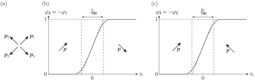
Figure 7: (a) Basis of spontaneous polarization states. Phase-field profiles of two 90^∘ domain walls: (b) charge-neutral wall; (c) charged wall, with properties discussed in Section 4.2.3.

This wall involves $\varphi_{1}$ and $\varphi_{4}$ satisfying $\varphi_{1}+\varphi_{4}=0$, while the other phase fields are identically zero. For simplicity we define $\varphi=\varphi_{4}$. A specialty of the polarization profile obtained from the general kinetics model is that the rotation of the polarization vector across the wall is predetermined by the decomposition (4.1), i.e.,

$$\overset{\ast}{\bm{p}}_{90}(\varphi)=\frac{p_{0}}{\sqrt{2}}\big{[}\tilde{\bm{e}}_{1}+(1-2\varphi)\tilde{\bm{e}}_{2}\big{]},$$ (4.40)

whereby $\bm{p}$ rotates with a constant component along $\tilde{\bm{e}}_{1}$. This is in contrast to the rotation of the polarization vector resulting from the Allen–Cahn model, which depends on the multi-well potential $\overline{\psi}_{s}$ given by (3.2), in particular on the parameter $\hat{\chi}$ introduced in (3.4), which determines the location of the 90^∘ barrier.

As a consequence, whereas in Section 3.2.4 the computed properties (wall width and interfacial energy) of the neutral 90^∘ domain wall are only approximations relying on the assumption that the $p_{1}$-component remains constant (a reasonable assumption for $\hat{\chi}=0.5$), for the general kinetics model these same properties characterize the neutral 90^∘ domain wall exactly.

Under the application of a uniform electric field $\bm{e}=e\tilde{\bm{e}}_{2}$ and with a derivation in all points analogous to that developed in Section 4.2.1, we conclude that the 90^∘ domain wall can be described by a traveling wave solution,

$$\varphi(x_{1},t)=\check{\varphi}(x_{1}-v_{90}t),$$ (4.41)

where $\xi=x_{1}-v_{90}t$ and $v_{90}$ is the velocity of the 90^∘ domain wall. Under the assumption that function $G_{90}$ is monotonous on $\mathbb{R}$, one can show that, akin to (4.21),

$$v_{90}=G_{90}(\sqrt{2}p_{0}e),$$ (4.42)

where $\sqrt{2}p_{0}e$ corresponds to the driving traction (2.22) associated with the 90^∘ configuration under consideration. Again, the polarization profile is given by (4.26) and (4.27) with a width $l_{90}=l/\sqrt{h_{90}}$ replacing $l$ and an interfacial energy $\Gamma_{90}=\sqrt{h_{90}}\Gamma$, which can be set to its physical value through a proper choice of $h_{90}$.

Charged domain wall

The transition from the neutral to the charged 90^∘ domain wall (see Figure 7(c)) shows the same features as the analogous transition for the 180^∘ domain wall. We discuss specifically the case $n=1$, for which the kinetic relation is exactly given by the function $G_{90}$, provided that $\zeta<2\sqrt{2}h_{90}$ is satisfied (like $\zeta<2$ for 180^∘ walls). The modified values of interfacial width and energy due to the regularization with $n=1$ are

$$l^{c}_{90}=l_{90}\left(1-\frac{\zeta}{2\sqrt{2}h_{90}}\right)^{-1/2}\qquad\mbox{and}\qquad\Gamma^{c}_{90}=\Gamma_{90}\left(1-\frac{\zeta}{2\sqrt{2}h_{90}}\right)^{1/2}.$$ (4.43)

4.3 Summary of the properties of 180^∘ and 90^∘ domain walls

Interface energy and width

We have computed exactly the interfacial energy and width of the different types of domain walls obtained with the general kinetics model. The expressions are analogous to those of the Allen–Cahn model. In particular, the choice of $C_{s}$ and $C_{g}$ allows us to set independently the interfacial energy and width (i.e., the regularization length) of 180^∘ domain walls, while $h_{90}$ determines the ratio of interfacial energy of 90^∘ and 180^∘ domain walls. Furthermore, the expressions for the interfacial properties of walls remain exact under an applied electric field, in contrast to the Allen–Cahn model for which one only has approximate expressions of interfacial properties when domain walls are not in equilibrium. This is notably related to the fact that, with the general kinetics model, values of the spontaneous polarization within domains are unchanged in the presence of an electric field.

Lastly, a special feature of the general kinetics model is that for 90^∘ domain walls the rotation of the polarization occurs with one of its components kept constant, as predetermined by the decomposition (4.1). This is in contrast to what happens with the Allen–Cahn model, where the rotation of $\bm{p}$ depends on the location of the 90^∘ barrier, given by $\hat{\chi}$ in the multi-well potential.

Kinetics

We have found that for straight domain walls the general kinetics model allows us to prescribe independently the kinetics of 180^∘ and 90^∘ domain walls and that these kinetic relations can be nonlinear. The kinetic relations (2.11) between the velocity of the interface (velocity of the traveling wave solutions) and the driving traction (computed from the values of the fields away from the diffuse interface) are defined through the functions $G_{180}$ and $G_{90}$ for 180^∘ and 90^∘ domain walls, respectively.

Interestingly, in the general kinetics model, the kinetic relation of straight walls is exactly given by $G_{180}$ and $G_{90}$ irrespective of the regularization length $l$, provided that $\zeta<2$ and $\zeta<2\sqrt{2}h_{90}$ are satisfied (i.e, $l$ is smaller than a critical length determined by the material parameters). This is in contrast to the Allen–Cahn model, for which the accuracy of the linear kinetic relations (3.27) and (3.35) for straight 180^∘ and 90^∘ domain walls decreases as the regularization length $l$ increases (because, as $l$ increases with constant material parameters, $e_{c}$ in (3.9) decreases, which reduces the accuracy of (3.27) and (3.35)).

As will be discussed in Part II of this study, when it comes to curved domain walls, the general kinetics model allows us to introduce the kinetic relations via $G_{180}$ and $G_{90}$ in an exact sense only in the limit of $l\rightarrow 0$ (see also the asymptotic analysis of Alber and Zhu (2013) for the phase-field model that inspired the present general kinetics model).

5 Conclusion

We have formulated a phase-field model for ferroelectrics that permits domain wall evolution with nonlinear kinetics, which we term the general kinetics model. Nonlinear domain wall kinetics is a crucial feature for properly accounting for rate effects in ferroelectric switching and is nonetheless absent from existing diffuse-interface ferroelectrics models. Seen in the general class of phase-field models for structural transformations (which includes switching between ferroelectric variants, twinning, solid-solid phase transformations), the general kinetics model is, to the best of our knowledge, the first diffuse-interface model with arbitrary nonlinear interface kinetics formulated for systems with multiple (i.e., more than two) phases. It has been devised as an extension to multiple phases of the hybrid model of Alber and Zhu (2013) (adapted here to the setting of ferroelectric switching).

To shed light on the new features of the general kinetics model, as compared to the classical Allen–Cahn-based phase-field model, we have worked in the simplified setting of rigid ferroelectrics, an assumption which only accounts for the electrostatic contribution to domain evolution and neglects the mechanical one. In this setting, we have compared two regularized models: the classical Allen–Cahn-based phase-field model and the newly introduced general kinetics model. By computing analytical traveling wave solutions for the propagation of straight 180^∘ and 90^∘ domain walls, both neutral and charged, we have established the following properties of the two phase-field models:

1. Interfacial width and energy: For both diffuse-interface models, the numerical parameters associated with the regularization of the electric enthalpy permit to set independently the interfacial energy of 180^∘ and 90^∘ domain walls and the width of 180^∘ domain walls. While the former are material parameters characterizing the walls, we see the latter as a numerical regularization length, whose choice is limited by practical constraints. With the Allen–Cahn model, interfacial width and energy weakly depend on the applied electric field and remain approximately constant in the regime (3.9) of $|\bm{e}|\ll\hat{e}_{c}$, with $\hat{e}_{c}=\hat{\Gamma}/(\hat{\eta}\hat{l}p_{0})$ a numerical characteristic electric field dependent on the regularization length $\hat{l}$. By contrast, with the general kinetics model, the interfacial width and energy of neutral domain walls are constant and independent of the applied electric field. As for charged domain walls (which encounter nonuniform electric fields induced by Gauss’ law), both models require, for wall properties to remain approximately independent of the regularization length, that the magnitude of the electric field associated with Gauss’ law remains small compared to a characteristic electric field. This translates into an upper bound on $\hat{l}$ and $l$, which reads as ${\hat{\eta}\hat{l}p_{0}^{2}}/({\epsilon\hat{\Gamma}})\ll 1$ (see (3.25)) for the Allen–Cahn model and ${\eta lp_{0}^{2}}/({\epsilon\Gamma})\ll 1$ for the general kinetics model (with quantitative estimates given in Sections 4.2.2 and 4.2.3).

2. Kinetics of domain walls: For the motion of straight 180^∘ and 90^∘ domain walls, we have shown that the Allen–Cahn formulation furnishes a regularization of a sharp-interface model with a linear kinetic relation between wall velocity and associated driving traction. In addition, while the kinetic coefficient associated with one type of domain walls (e.g., 180^∘ domain wall) can be freely set with a proper choice of the inverse mobility $\mu$ in (3.6), that of the other type of wall (e.g., 90^∘ domain wall) is automatically prescribed by the ratio of interfacial energies of the two types of domain walls. Furthermore, the Allen–Cahn model only furnishes an approximately linear kinetics behavior valid in the regime where both (3.9) and (3.25) are satisfied.

   The general kinetics model, by contrast, provides a regularization of the sharp-interface model with arbitrary kinetic relations given by the functions $G_{180}$ and $G_{90}$ for 180^∘ and 90^∘ domain walls, respectively. More specifically, for straight walls of all types, we have shown with traveling wave solutions that the relations between wall velocities and associated driving tractions are exactly given by $G_{180}$ and $G_{90}$, provided that the (little restrictive) conditions $\zeta<2$ and $\zeta<2\sqrt{2}h_{90}$ are satisfied. Overall, they again furnish upper bounds on the regularization length $l$.

In the present article, we have focused on analytically tractable features of the Allen–Cahn and general kinetics models. For that reason, we have restricted our attention to the properties and motion of straight domain walls. With this focus, we made the important clarification that with the Allen–Cahn model, the target kinetics is attained only in the limit of $\hat{l}\rightarrow 0$, while the general kinetics model furnishes exactly the chosen kinetics, irrespective of the regularization length, provided the latter satisfies specific upper bounds. We point out that, although our discussion was specific to ferroelectric domain wall motion, the same general kinetics model bears potential for other applications involving structural transformations.

In a follow-up publication, we will report a numerical implementation of the general kinetics model and address the propagation of curved walls as well as the behavior of triple and quadruple points where multiple phases meet.

Appendix A Experimental evidence on domain wall dynamics

180^∘ domain walls

Experimental and theoretical works have probed the kinetics of domain walls both in bulk single-crystals and in thin films (for an extensive review of these works, see Tagantsev et al. 2010). Here, we summarize results pertaining only to bulk BaTiO₃. The velocity of non-ferroelastic 180^∘ domains walls was measured as a function of the electric field in single-crystal BaTiO₃ by Miller and Savage (1958, 1959, 1960); Savage and Miller (1960) for electric fields in the range 0.1 to 2$\,\mathrm{kV/cm}$ and by Stadler and Zachmanidis (1963) at large fields between 2 and 450$\,\mathrm{kV/cm}$. These experiments were performed on plate-like samples with polarization and electric field oriented along the out-of-plane $\tilde{\bm{e}}_{z}$-direction. As a result, the electric field $\bm{e}=e\tilde{\bm{e}}_{z}$ is uniform throughout the sample and the driving traction given by (2.9) reduces to $f=2p_{0}e$ for an interface with negligible curvature. For electric fields in the range $0.1$ to $2\,\mathrm{kV/cm}$, an inverse exponential dependence of the domain wall velocity on the electric field was inferred:

$$V_{180}(e)=V_{l}\exp(-e_{a}/e),$$ (A.1)

where $V_{l}$ is a characteristic velocity of the order of $100\,\mathrm{cm/s}$, and the activation field $e_{a}$ is typically about $4\,\mathrm{kV/cm}$ at room temperature (Miller and Savage, 1960). The exact value of these parameters depends on temperature, sample thickness, the presence of defects, and the nature of the electrodes. These observations suggest that for 180^∘ domain walls in the range $f\leq 1\times 10^{5}\,\mathrm{J/m^{3}}$ (cf. $p_{0}=0.26\,\mathrm{C/m^{2}}$), the driving traction follows a kinetic relation of inverse-exponential type, given by

$$V_{180}(f)=\operatorname{sgn}(f)V_{l}\exp(-f_{a}/|f|),$$ (A.2)

where $f_{a}=2p_{0}e_{a}$ is an activation driving traction. Above 2$\,\mathrm{kV/cm}$ the velocity was found to follow a power law $V_{180}\propto e^{\theta}$ with $\theta=1.4$ (Stadler and Zachmanidis, 1963), which indicates for $f>1\times 10^{5}\,\mathrm{J/m^{3}}$ a kinetic relation of the form

$$V_{180}(f)=\operatorname{sgn}(f)V_{h}\left(\frac{|f|}{f_{a}}\right)^{\theta},$$ (A.3)

with $V_{h}$ a characteristic velocity for large driving tractions.

90^∘ domain walls

While experimental data for the motion of 90^∘ domain walls in BaTiO₃ are lacking, observations of the kinetics of ferroelastic domain walls in other materials (Rochelle salt, galodinium molybdate, potassium dihydrogen phosphate as reviewed in Tagantsev et al. (2010), Section 8.3.3) point to a different kinetic relation specific to ferroleastic domain walls. Indeed, irrespective of the material, it appears that ferroelastic walls remain static for applied electric fields smaller than a threshold field, above which their velocity evolves linearly with the field. This suggests a threshold-type linear relation:

$$V_{90}(f)=\begin{cases}0\quad&\mbox{for}\quad|f|<f_{0},\\ \operatorname{sgn}(f)k(|f|-f_{0})&\mbox{for}\quad|f|\geq f_{0},\end{cases}$$ (A.4)

where $f_{0}$ is a threshold driving traction and $k$ a kinetic coefficient. At the same time, ab initio calculations by Liu et al. (2016) have shown that 90^∘ domain walls in PbTiO₃ exhibit the same two-regime kinetics as that observed for 180^∘ domain walls in BaTiO₃ and described by (A.2) and (A.3) in the regimes of small and large electric fields, respectively. While we unfortunately do not have a full set of data for the kinetics of the different kinds of domain walls in one particular material, current observations clearly indicate that the kinetics of domain walls is nonlinear and dependent on the type of domain wall (i.e., non-ferroelastic vs. ferroelastic).

References

- Abeyaratne and Knowles (1990) Abeyaratne, R., Knowles, J.K., 1990. On the driving traction acting on a surface of strain discontinuity in a continuum. Journal of the Mechanics and Physics of Solids 38, 345–360. doi:doi:10.1016/0022-5096(90)90003-m.
- Abeyaratne and Knowles (2006) Abeyaratne, R., Knowles, J.K., 2006. Evolution of Phase Transitions. Cambridge University Press. doi:doi:10.1017/cbo9780511547133.
- Agrawal (2016) Agrawal, V., 2016. Multiscale Phase-field Model for Phase Transformation and Fracture. Ph.D. thesis. Carnegie Mellon University. URL: https://kilthub.cmu.edu/articles/thesis/Multiscale_Phase-field_Model_for_Phase_Transformation_and_Fracture/6720785.
- Agrawal and Dayal (2015a) Agrawal, V., Dayal, K., 2015a. A dynamic phase-field model for structural transformations and twinning: Regularized interfaces with transparent prescription of complex kinetics and nucleation. part i: Formulation and one-dimensional characterization. Journal of the Mechanics and Physics of Solids 85, 270–290. doi:doi:10.1016/j.jmps.2015.04.010.
- Agrawal and Dayal (2015b) Agrawal, V., Dayal, K., 2015b. A dynamic phase-field model for structural transformations and twinning: Regularized interfaces with transparent prescription of complex kinetics and nucleation. part II: Two-dimensional characterization and boundary kinetics. Journal of the Mechanics and Physics of Solids 85, 291–307. doi:doi:10.1016/j.jmps.2015.05.001.
- Ahluwalia and Cao (2001) Ahluwalia, R., Cao, W., 2001. Size dependence of domain patterns in a constrained ferroelectric system. Journal of Applied Physics 89, 8105–8109. doi:doi:10.1063/1.1371282.
- Alber and Zhu (2005) Alber, H.D., Zhu, P., 2005. Solutions to a model with nonuniformly parabolic terms for phase evolution driven by configurational forces. SIAM Journal on Applied Mathematics 66, 680–699. doi:doi:10.1137/050629951.
- Alber and Zhu (2007) Alber, H.D., Zhu, P., 2007. Evolution of phase boundaries by configurational forces. Archive for Rational Mechanics and Analysis 185, 235–286. doi:doi:10.1007/s00205-007-0054-8.
- Alber and Zhu (2013) Alber, H.D., Zhu, P., 2013. Comparison of a rapidely converging phase field model for interfaces in solids with the allen-cahn model. Journal of Elasticity 111, 153–221. doi:doi:10.1007/s10659-012-9398-x.
- Allen and Cahn (1979) Allen, S.M., Cahn, J.W., 1979. A microscopic theory for antiphase boundary motion and its application to antiphase domain coarsening. Acta Metallurgica 27, 1085–1095. doi:doi:10.1016/0001-6160(79)90196-2.
- Arlt and Sasko (1980) Arlt, G., Sasko, P., 1980. Domain configuration and equilibrium size of domains in BaTiO3ceramics. Journal of Applied Physics 51, 4956–4960. doi:doi:10.1063/1.328372.
- Brainerd (1949) Brainerd, J.G., 1949. Standards on piezoelectric crystals, 1949. Proceedings of the IRE 37, 1378–1395. doi:doi:10.1109/JRPROC.1949.229975.
- Bulaevskii and Ginzburg (1964) Bulaevskii, L.N., Ginzburg, V.L., 1964. Temperature dependence of the shape of the domain wall in ferromagnetics and ferroelectrics. Soviet Physics JETP 18, 5.
- Cao and Cross (1991) Cao, W., Cross, L.E., 1991. Theory of tetragonal twin structures in ferroelectric perovskites with a first-order phase transition. Physical Review B 44, 5–12. doi:doi:10.1103/physrevb.44.5.
- Chen et al. (2011) Chen, X., Dong, X., Zhang, H., Cao, F., Wang, G., Gu, Y., He, H., Liu, Y., 2011. Frequency dependence of coercive field in soft pb(zr1-xTix)o3 (0.20 x 0.60) bulk ceramics. Journal of the American Ceramic Society 94, 4165–4168. doi:doi:10.1111/j.1551-2916.2011.04913.x.
- Flaschel and De Lorenzis (2020) Flaschel, M., De Lorenzis, L., 2020. Calibration of material parameters based on 180$$^\circ $$ and 90$$^\circ $$ ferroelectric domain wall properties in ginzburg–landau–devonshire phase field models. Archive of Applied Mechanics 90, 2755–2774. doi:doi:10.1007/s00419-020-01747-7.
- Fried and Gurtin (1994) Fried, E., Gurtin, M., 1994. Dynamic solid-solid transitions with phase characterized by an order parameter. Physica D: Nonlinear Phenomena 72, 287–308. doi:doi:10.1016/0167-2789(94)90234-8.
- Genenko et al. (2012) Genenko, Y.A., Zhukov, S., Yampolskii, S.V., Schütrumpf, J., Dittmer, R., Jo, W., Kungl, H., Hoffmann, M.J., von Seggern, H., 2012. Universal polarization switching behavior of disordered ferroelectrics. Advanced Functional Materials 22, 2058–2066. doi:doi:10.1002/adfm.201102841.
- Gordon (1986) Gordon, A., 1986. Interface motion in ferroelectrics. Physica B+C 138, 239–243. doi:doi:10.1016/0378-4363(86)90002-1.
- Gurtin (1993) Gurtin, M.E., 1993. Thermomechanics of evolving phase boundaries in the plane.
- Gurtin (2000) Gurtin, M.E., 2000. Configurational Forces as Basic Concepts of Continuum Physics. Springer New York. doi:doi:10.1007/b97847.
- Gurtin et al. (2009) Gurtin, M.E., Fried, E., Anand, L., 2009. The Mechanics and Thermodynamics of Continua. Cambridge University Press. doi:doi:10.1017/cbo9780511762956.
- Hou et al. (1999) Hou, T.Y., Rosakis, P., LeFloch, P., 1999. A level-set approach to the computation of twinning and phase-transition dynamics. Journal of Computational Physics 150, 302–331. doi:doi:10.1006/jcph.1998.6179.
- Hu and Chen (1997) Hu, H.L., Chen, L.Q., 1997. Computer simulation of 90 ° ferroelectric domain formation in two-dimensions. Materials Science and Engineering: A 238, 182–191. doi:doi:10.1016/s0921-5093(97)00453-x.
- Hu and Chen (1998) Hu, H.L., Chen, L.Q., 1998. Three-dimensional computer simulation of ferroelectric domain formation. Journal of the American Ceramic Society 81, 492–500. doi:doi:10.1111/j.1151-2916.1998.tb02367.x.
- Hubmann et al. (2016) Hubmann, A.H., Li, S., Zhukov, S., von Seggern, H., Klein, A., 2016. Polarisation dependence of schottky barrier heights at ferroelectric BaTiO3 / RuO2interfaces: influence of substrate orientation and quality. Journal of Physics D: Applied Physics 49, 295304. doi:doi:10.1088/0022-3727/49/29/295304.
- Indergand (2019) Indergand, R., 2019. Finite-Temperature Phase Field Simulations of Ferroelectric Ceramics (Unpublished). Master’s thesis. ETH Zurich.
- Indergand et al. (2020) Indergand, R., Vidyasagar, A., Nadkarni, N., Kochmann, D.M., 2020. A phase-field approach to studying the temperature-dependent ferroelectric response of bulk polycrystalline PZT. Journal of the Mechanics and Physics of Solids 144, 104098. doi:doi:10.1016/j.jmps.2020.104098.
- Ishiwara et al. (2004) Ishiwara, H., Okuyama, M., Arimoto, Y. (Eds.), 2004. Ferroelectric Random Access Memories. Springer Berlin Heidelberg. doi:doi:10.1007/b12953.
- Jiang (1994a) Jiang, Q., 1994a. On modeling of phase transformations in ferroelectric materials. Acta Mechanica 102, 149–165. doi:doi:10.1007/bf01178524.
- Jiang (1994b) Jiang, Q., 1994b. On the driving traction acting on a surface of discontinuity within a continuum in the presence of electromagnetic fields. Journal of Elasticity 34, 1–21. doi:doi:10.1007/bf00042423.
- Jo et al. (2009) Jo, J.Y., Yang, S.M., Kim, T.H., Lee, H.N., Yoon, J.G., Park, S., Jo, Y., Jung, M.H., Noh, T.W., 2009. Nonlinear dynamics of domain-wall propagation in epitaxial ferroelectric thin films. Physical Review Letters 102. doi:doi:10.1103/physrevlett.102.045701.
- Kamlah (2001) Kamlah, M., 2001. Ferroelectric and ferroelastic piezoceramics – modeling of electromechanical hysteresis phenomena. Continuum Mechanics and Thermodynamics 13, 219–268. doi:doi:10.1007/s001610100052.
- Kannan et al. (2022) Kannan, V., Trassin, M., Kochmann, D.M., 2022. Kinetics of ferroelectric switching in poled barium titanate ceramics: Effects of electrical cycling rate. Materialia 25, 101553. doi:doi:10.1016/j.mtla.2022.101553.
- Kessler and Balke (2006) Kessler, H., Balke, H., 2006. A continuum analysis of the driving force of ferroelectric/ferroelastic domain wall motions. Journal of the Mechanics and Physics of Solids 54, 113–127. doi:doi:10.1016/j.jmps.2005.08.004.
- Landau and Lifshitz (1935) Landau, L.D., Lifshitz, E., 1935. On the theory of the dispersion of magnetic permeability in ferromagnetic bodies. Phys. Zeitsch. der Sowjet. 8, 153–169. URL: http://cds.cern.ch/record/437299.
- Li et al. (2001) Li, Y.L., Hu, S.Y., Liu, Z.K., Chen, L.Q., 2001. Phase-field model of domain structures in ferroelectric thin films. Applied Physics Letters 78, 3878–3880. doi:doi:10.1063/1.1377855.
- Little (1955) Little, E.A., 1955. Dynamic behavior of domain walls in barium titanate. Physical Review 98, 978–984. doi:doi:10.1103/physrev.98.978.
- Liu et al. (2016) Liu, S., Grinberg, I., Rappe, A.M., 2016. Intrinsic ferroelectric switching from first principles. Nature 534, 360–363. doi:doi:10.1038/nature18286.
- Loge and Suo (1996) Loge, R., Suo, Z., 1996. Nonequilibrium thermodynamics of ferroelectric domain evolution. Acta Materialia 44, 3429–3438. doi:doi:10.1016/1359-6454(95)00425-4.
- Merz (1954) Merz, W.J., 1954. Domain formation and domain wall motions in ferroelectric BaTiO3single crystals. Physical Review 95, 690–698. doi:doi:10.1103/physrev.95.690.
- Merz (1956) Merz, W.J., 1956. Switching time in ferroelectric BaTiO3 and its dependence on crystal thickness. Journal of Applied Physics 27, 938–943. doi:doi:10.1063/1.1722518.
- Miller and Savage (1958) Miller, R.C., Savage, A., 1958. Velocity of sidewise 180° domain-wall motion in BaTiO3as a function of the applied electric field. Physical Review 112, 755–762. doi:doi:10.1103/physrev.112.755.
- Miller and Savage (1959) Miller, R.C., Savage, A., 1959. Further experiments on the sidewise motion of 180° domain walls in BaTiO3. Physical Review 115, 1176–1180. doi:doi:10.1103/physrev.115.1176.
- Miller and Savage (1960) Miller, R.C., Savage, A., 1960. Motion of 180° domain walls in metal electroded barium titanate crystals as a function of electric field and sample thickness. Journal of Applied Physics 31, 662–669. doi:doi:10.1063/1.1735663.
- Miller and Weinreich (1960) Miller, R.C., Weinreich, G., 1960. Mechanism for the sidewise motion of 180° domain walls in barium titanate. Physical Review 117, 1460–1466. doi:doi:10.1103/physrev.117.1460.
- Mueller et al. (2006) Mueller, R., Gross, D., Lupascu, D., 2006. Driving forces on domain walls in ferroelectric materials and interaction with defects. Computational Materials Science 35, 42–52. doi:doi:10.1016/j.commatsci.2005.02.014.
- Nambu and Sagala (1994) Nambu, S., Sagala, D.A., 1994. Domain formation and elastic long-range interaction in ferroelectric perovskites. Physical Review B 50, 5838–5847. doi:doi:10.1103/physrevb.50.5838.
- Osher and Sethian (1988) Osher, S., Sethian, J.A., 1988. Fronts propagating with curvature-dependent speed: Algorithms based on hamilton-jacobi formulations. Journal of Computational Physics 79, 12–49. doi:doi:10.1016/0021-9991(88)90002-2.
- Rezaee-Hajidehi and Stupkiewicz (2021) Rezaee-Hajidehi, M., Stupkiewicz, S., 2021. Micromorphic approach to phase-field modeling of multivariant martensitic transformation with rate-independent dissipation effects. International Journal of Solids and Structures 222-223, 111027. URL: https://doi.org/10.1016%2Fj.ijsolstr.2021.03.014, doi:doi:10.1016/j.ijsolstr.2021.03.014.
- Rosakis and Jiang (1995) Rosakis, P., Jiang, Q., 1995. On the morphology of ferroelectric domains. International Journal of Engineering Science 33, 1–12. doi:doi:10.1016/0020-7225(94)e0039-l.
- Savage and Miller (1960) Savage, A., Miller, R.C., 1960. Temperature dependence of the velocity of sidewise 180° domain-wall motion in BaTiO3. Journal of Applied Physics 31, 1546–1549. doi:doi:10.1063/1.1735890.
- Schmidt (1981) Schmidt, N.A., 1981. Coercive force and 90° domain wall motion in ferroelectric PLZT ceramics with square hysteresis loops. Ferroelectrics 31, 105–111. doi:doi:10.1080/00150198108201980.
- Schrade et al. (2013) Schrade, D., Müller, R., Gross, D., 2013. On the physical interpretation of material parameters in phase field models for ferroelectrics. Archive of Applied Mechanics 83, 1393–1413. doi:doi:10.1007/s00419-013-0754-5.
- Schrade et al. (2014) Schrade, D., Müller, R., Gross, D., Keip, M.A., Thai, H., Schröder, J., 2014. An invariant formulation for phase field models in ferroelectrics. International Journal of Solids and Structures 51, 2144–2156. doi:doi:10.1016/j.ijsolstr.2014.02.021.
- Schultheiß et al. (2019) Schultheiß, J., Kungl, H., Koruza, J., 2019. Influence of crystallographic structure on polarization reversal in polycrystalline ferroelectric/ferroelastic materials. Journal of Applied Physics 125, 174101. doi:doi:10.1063/1.5081086.
- Schultheiß et al. (2018) Schultheiß, J., Liu, L., Kungl, H., Weber, M., Venkataraman, L.K., Checchia, S., Damjanovic, D., Daniels, J.E., Koruza, J., 2018. Revealing the sequence of switching mechanisms in polycrystalline ferroelectric/ferroelastic materials. Acta Materialia 157, 355–363. doi:doi:10.1016/j.actamat.2018.07.018.
- Shin et al. (2007) Shin, Y.H., Grinberg, I., Chen, I.W., Rappe, A.M., 2007. Nucleation and growth mechanism of ferroelectric domain-wall motion. Nature 449, 881–884. doi:doi:10.1038/nature06165.
- Stadler and Zachmanidis (1963) Stadler, H.L., Zachmanidis, P.J., 1963. Nucleation and growth of ferroelectric domains in BaTiO3 at fields from 2 to 450 kV/cm. Journal of Applied Physics 34, 3255–3260. doi:doi:10.1063/1.1729173.
- Su and Landis (2007) Su, Y., Landis, C.M., 2007. Continuum thermodynamics of ferroelectric domain evolution: Theory, finite element implementation, and application to domain wall pinning. Journal of the Mechanics and Physics of Solids 55, 280–305. doi:doi:10.1016/j.jmps.2006.07.006.
- Tagantsev et al. (2010) Tagantsev, A.K., Cross, L.E., Fousek, J., 2010. Domains in Ferroic Crystals and Thin Films. Springer New York. doi:doi:10.1007/978-1-4419-1417-0.
- Truskinovsky (1987) Truskinovsky, L., 1987. Dynamics of non-equilibrium phase boundaries in a heat conducting non-linearly elastic medium. Journal of Applied Mathematics and Mechanics 51, 777–784. doi:doi:10.1016/0021-8928(87)90140-7.
- Tůma et al. (2018) Tůma, K., Stupkiewicz, S., Petryk, H., 2018. Rate-independent dissipation in phase-field modelling of displacive transformations. Journal of the Mechanics and Physics of Solids 114, 117–142. doi:doi:10.1016/j.jmps.2018.02.007.
- Tybell et al. (2002) Tybell, T., Paruch, P., Giamarchi, T., Triscone, J.M., 2002. Domain wall creep in epitaxial FerroelectricPb(zr0.2ti0.8)o3thin films. Physical Review Letters 89. doi:doi:10.1103/physrevlett.89.097601.
- Uchino (2018) Uchino, K., 2018. Ferroelectric devices. CRC press.
- Vidyasagar et al. (2017) Vidyasagar, A., Tan, W., Kochmann, D., 2017. Predicting the effective response of bulk polycrystalline ferroelectric ceramics via improved spectral phase field methods. Journal of the Mechanics and Physics of Solids 106, 133–151. doi:doi:10.1016/j.jmps.2017.05.017.
- Wieder (1957) Wieder, H.H., 1957. Activation field and coercivity of ferroelectric barium titanate. Journal of Applied Physics 28, 367–369. doi:doi:10.1063/1.1722749.
- Yang and Chen (1995) Yang, W., Chen, L.Q., 1995. Computer simulation of the dynamics of 180o ferroelectric domains. Journal of the American Ceramic Society 78, 2554–2556. doi:doi:10.1111/j.1151-2916.1995.tb08702.x.
- Yin and Cao (2002) Yin, J., Cao, W., 2002. Coercive field of 0.955pb(zn1/3nb2/3)o3–0.045pbtio3 single crystal and its frequency dependence. Applied Physics Letters 80, 1043–1045. doi:doi:10.1063/1.1448385.
- Zhang and Bhattacharya (2005a) Zhang, W., Bhattacharya, K., 2005a. A computational model of ferroelectric domains. part i: model formulation and domain switching. Acta Materialia 53, 185–198. doi:doi:10.1016/j.actamat.2004.09.016.
- Zhang and Bhattacharya (2005b) Zhang, W., Bhattacharya, K., 2005b. A computational model of ferroelectric domains. part II: grain boundaries and defect pinning. Acta Materialia 53, 199–209. doi:doi:10.1016/j.actamat.2004.09.015.
- Zhirnov (1959) Zhirnov, V.A., 1959. A contribution to the theory of domain walls in ferroelectrics. Soviet Physics JETP 35, 822–827.