Concept Evolution in Deep Learning Training:
A Unified Interpretation Framework and Discoveries

Abstract.

We present ConceptEvo, a unified interpretation framework for deep neural networks (DNNs) that reveals the inception and evolution of learned concepts during training. Our work addresses a critical gap in DNN interpretation research, as existing methods primarily focus on post-training interpretation. ConceptEvo introduces two novel technical contributions: (1) an algorithm that generates a unified semantic space, enabling side-by-side comparison of different models during training, and (2) an algorithm that discovers and quantifies important concept evolutions for class predictions. Through a large-scale human evaluation and quantitative experiments, we demonstrate that ConceptEvo successfully identifies concept evolutions across different models, which are not only comprehensible to humans but also crucial for class predictions. ConceptEvo is applicable to both modern DNN architectures, such as ConvNeXt, and classic DNNs, such as VGGs and InceptionV3.

1. Introduction

Interpreting how Deep Neural Networks (DNNs) arrive at their decisions has become crucial for instilling trust in the models (Ribeiro et al., 2016), debugging them (Koh and Liang, 2017), and guarding against potential harms such as embedded bias or adversarial attacks (Das et al., 2020; Papernot and McDaniel, 2018; Zhang et al., 2018). As a fundamental type of DNN, convolutional neural networks have garnered significant interest in understanding their internal mechanism. Saliency-based interpretation methods, for example, aim to identify important image regions for predictions (Selvaraju et al., 2017; Simonyan et al., 2013). Concept-based interpretation methods identify concepts detected by DNNs, such as “dog face” concepts shown in Fig 1, and their role in forming higher-level concepts and predictions (Park et al., 2021; Olah et al., 2020; Ghorbani et al., 2019; Kim et al., 2018; Bau et al., 2017). These methods connect a concept with sets of images or image patches that explain the concept, using shared visual characteristics among the images to enhance human understanding of the concept (Chen et al., 2019; Olah et al., 2017; Ghorbani et al., 2019). Neuron-level concept interpretation methods focus on concepts that elicit strong activation in that neuron (Olah et al., 2017; Chen et al., 2019; Park et al., 2021).

However, existing interpretation approaches mostly focus on post-training analysis (Laugel et al., 2019; Guidotti et al., 2018), providing limited insights into the evolution of models during training. Crucially, understanding the progression of concepts detected by individual neurons, which we refer to as the neuron’s concept evolution, and its association with model deficiencies like poor generalizability (Li et al., 2018; Zhang et al., 2021; Keskar et al., 2017) or convergence failures (Reddi et al., 2019; Arora et al., 2019) remains lacking. Relying solely on post-training interpretation poses challenges for real-time discovery and diagnosis during training, potentially wasting time and resources (Elsken et al., 2019; Safarik et al., 2018), if the training ultimately fails to achieve desired outcomes. Interpreting the DNN training process also enhances effective monitoring (Zhong et al., 2017; Liu et al., 2017; Abadi et al., 2016; Zhou et al., 2022).

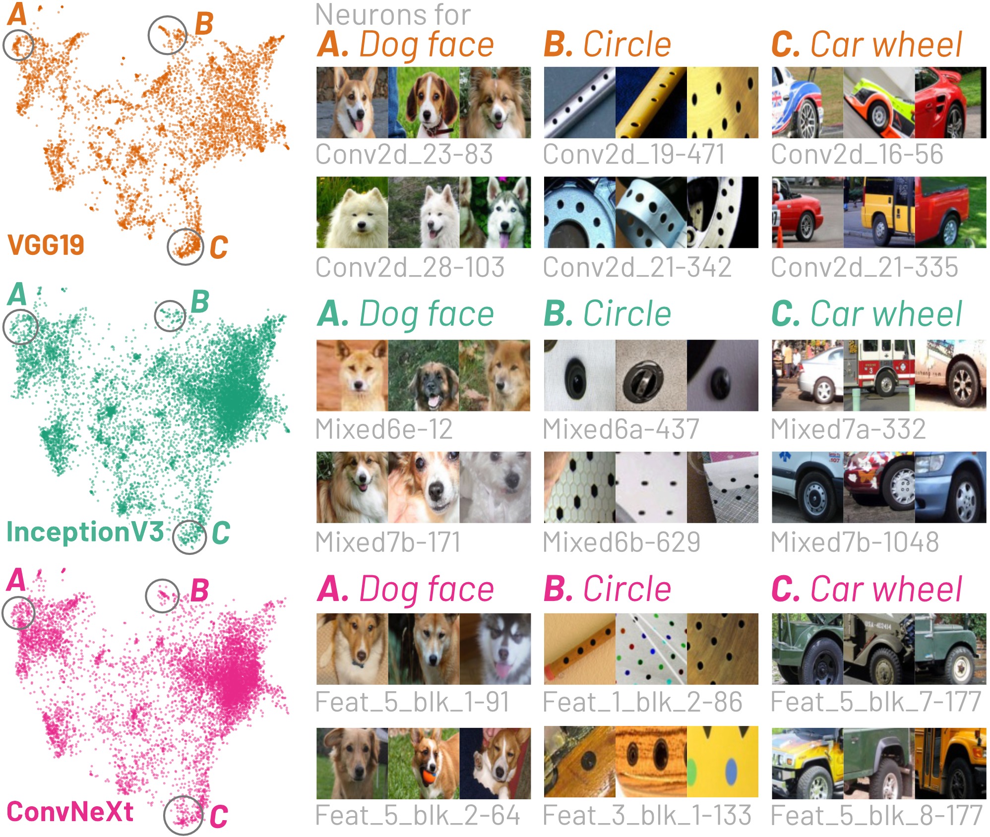
Figure 1. ConceptEvo creates a unified semantic space that enables side-by-side comparison of different models during training (top: VGG19; middle: InceptionV3; bottom: ConvNeXt). ConceptEvo embeds and aligns neurons (dots) that detect similar concepts (e.g., dog face, circle, car wheel) to similar locations.

To fill these gaps, our work contributes as follows:

1. ConceptEvo, a unified interpretation framework that reveals the inception and evolution of concepts during DNN training (Sec 3), with two novel technical contributions:

   • An algorithm that generates a unified semantic space that enables side-by-side comparison of different models during training (Fig 1, 2). ConceptEvo is applicable to both modern ConvNeXt and classic DNNs like VGGs and InceptionV3.

   • An algorithm that discovers and quantifies important concept evolutions for class predictions (Fig 3).

2. Extensive evaluation (Sec 4). A large-scale human experiments with 260 participants and quantitative experiments demonstrate that ConceptEvo identifies concept evolutions that are not only meaningful to humans but also important for class predictions.

3. Discoveries on model evolution (Sec 4.5). We highlight how ConceptEvo aids in uncovering potential issues during model training and provides insights into their causes, such as: (1) severely harmed concept diversity caused by incompatible hyperparameters (e.g., overly high learning rate) as shown in Fig 2b; and (2) slowly evolving concepts despite rapid increases in training accuracy in overfitted model as shown in Fig 2c.

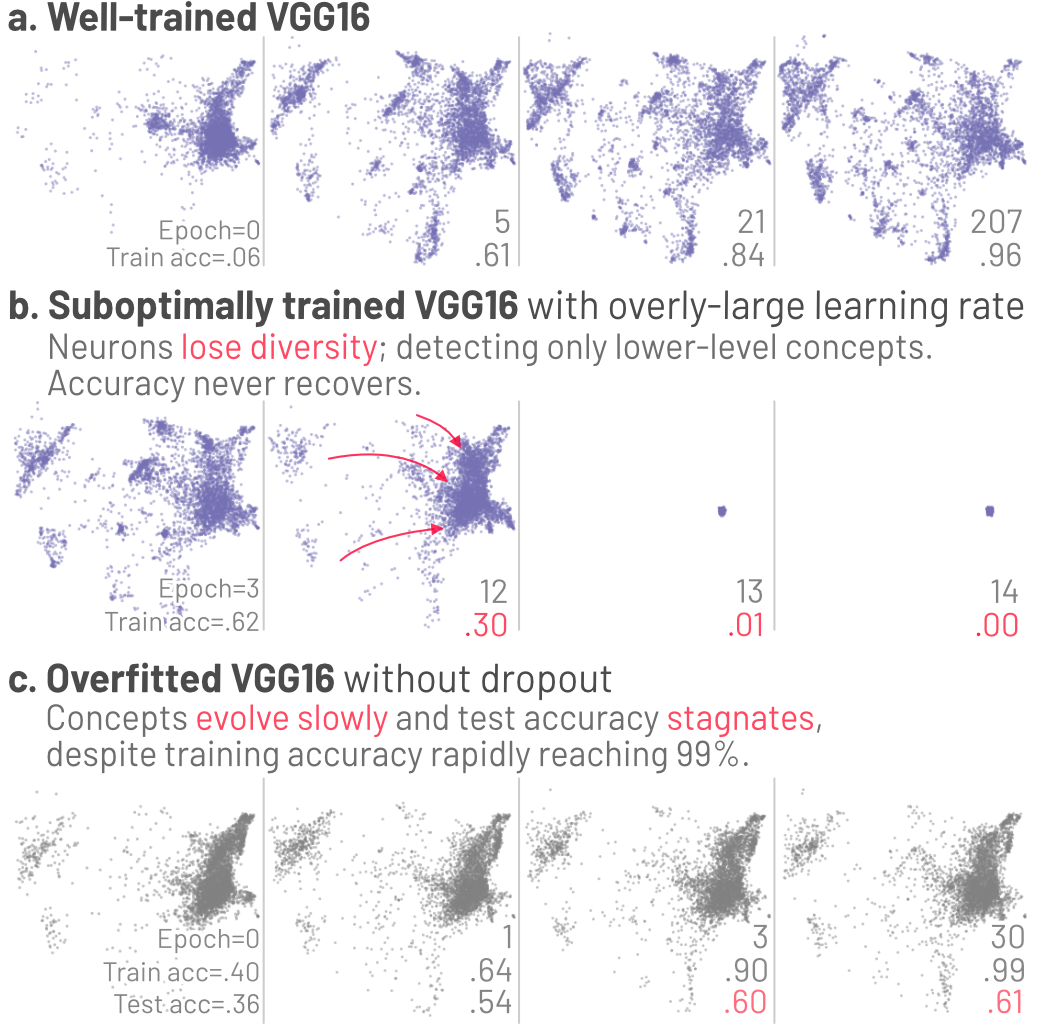
Figure 2. ConceptEvo identifies potential training issues. (a) A well-trained VGG16 shows gradual concept formations and refinements. (b) A VGG16 suboptimally trained with a large learning rate, rapidly losing the ability to detect most concepts. (c) An overfitted VGG16 without dropout layers, showing slow concept evolutions despite rapid training accuracy increases. We abbreviate “top-5 training/test accuracies” as “train/test acc.”

2. Related Work

Interpreting DNNs After Training. Interpreting fully-trained DNNs revolves around describing crucial features of models’ behavior. For example, saliency-based methods identify image pixels that are important for predictions (Simonyan et al., 2013; Simonyan and Zisserman, 2015; Gan et al., 2015; Selvaraju et al., 2017). However, these methods face a challenge as important image pixels may not align with high-level concepts that are easily understandable to humans (Kim et al., 2018; Gulshad and Smeulders, 2020). To address this, recent studies have focused on explaining high-level, human-understandable concepts learned within DNNs and their relevance to the models’ prediction (Hernandez et al., 2022; Ghorbani and Zou, 2020; Yeh et al., 2020; Goyal et al., 2019; Zhou et al., 2018; Kim et al., 2018; Nguyen et al., 2016). For example, feature visualization techniques (Zeiler and Fergus, 2014; Yosinski et al., 2015) generate synthetic images that strongly activate specific neurons, visualizing detected concepts. ACE (Ghorbani et al., 2019) discovers important image segmentations, presenting learned concepts that are important for predictions. Net2Vec (Fong and Vedaldi, 2018) encodes individual neurons’ concepts into vectors by using predefined concept images. MILAN (Hernandez et al., 2022) explains learned concepts through short natural language descriptions. NeuroCartography (Park et al., 2021) visualizes concepts detected by neurons through encoding the conceptual neighborhood of neurons.

Interpreting DNNs During Training. Several existing studies that aim to interpret DNNs during training focus on the evolution of data representations within the models across epochs and how this evolution influences their downstream performance (Pühringer et al., 2020; Smilkov et al., 2017; Chung et al., 2016). DeepEyes (Pezzotti et al., 2017) examines the evolution of individual neurons’ activation for different classes during training. DGMTracker (Liu et al., 2017) analyzes changes in weights, activations, and gradients over time. Other approaches track the 2D projected evolution of neurons towards or away from specific labels (Rauber et al., 2016; Li et al., 2020), although this limits our understanding of learned concepts to the available labels only. DeepView (Zhong et al., 2017) introduces metrics to estimate whether neurons are evolving sufficient diversity for classification. ConceptEvo distinguishes itself from the existing approaches by enabling the comparison of concepts learned by neurons from any layer within a model and even by neurons from different models.

3. Method

3.1. Desiderata of Interpreting Concept Evolution

1. General interpretation of concept evolution across different models. Comparing the training of different models is essential for determining which model is trained better or which training strategy is more effective (Li et al., 2018; Raghu et al., 2017). Thus, we aim to develop a general method that enables side-by-side comparison and interpretation of concept evolution across different models. (Sec 3.2)

2. Revealing and quantifying important evolution of concepts. We aim to identify internal changes that significantly impact the prediction of a specific class, as understanding the most influential components can lead to effective model improvements (Ghorbani and Zou, 2020). For example, we seek to determine the importance of a neuron’s concept evolution, such as the transition from “brown color” to “brown furry leg” in the prediction of a “brown bear” class. We aim to automatically discover these important changes in concepts for class predictions. (Sec 3.3)

3. Discoveries. Can the interpretation of how a model evolves help identify training problems and provide insights for addressing them, advancing prior work that focuses on interpreting and fixing models post-training (Ghorbani and Zou, 2020)? For example, can we help determine if a model’s training is on the right track and if interventions are necessary to improve accuracy? (Sec 4.5)

3.2. General Interpretation of Concept Evolution

We desire an interpretation of model evolution that is comparable across different models. However, direct comparison between concepts in different models at different training stages is challenging. Different models are independently trained; thus, the learned concepts are not aligned by default. Even for the same model, activation patterns can change considerably over training epochs.

To address this challenge, we propose a two-step method. In step 1, we create a base semantic space that captures the concepts identified by a base model at a specific training epoch. This semantic space serves as a fundamental reference for concept representation. In step 2, we project the concepts from other models spanning all epochs onto the base semantic space, resulting in a unified semantic space where similar concepts across different models and epochs are mapped to similar locations.

We choose an optimally, fully trained model as our base model to ensure broad concept coverage. For example, we used a fully trained VGG19 (Simonyan and Zisserman, 2015) as the base model for Fig 1 and 2.

Step 1: Creating the base semantic space. To create the base semantic space, we use neurons as a unit to identify and represent concepts, inspired by studies that demonstrate neurons’ selective activation for specific concepts (Ghorbani and Zou, 2020; Olah et al., 2017; Yosinski et al., 2015). By using neurons, we can pinpoint areas of interest in models, enabling focused troubleshooting, particularly in identifying abnormal training patterns within specific groups of neurons. Building on prior work (Park et al., 2021), we embed neurons that strongly respond to common inputs in similar locations. As neuron-concept relationships may not always be one-to-one (Olah et al., 2020; Fong and Vedaldi, 2018), we aim to generalize to many-to-many relationships. For example, polysemantic neurons responsive to multiple concepts are embedded between those concepts.

Step 1.1: Finding stimuli. ConceptEvo creates stimuli for each neuron by collecting a set of $k$ images that result in the highest maximum in the neuron’s activation map. For neurons associated with a single concept, their stimuli will be more alike, while for polysemantic neurons, their stimuli may consist of multiple concepts.

Step 1.2: Sampling frequently co-activated neuron pairs. ConceptEvo creates a multiset $D$, which consists of sampled pairs of strongly co-activated neurons from the base model $M_{b}$ at epoch $t_{b}$. First, for each image $\mathbf{x}$, it creates a list of neurons that are strongly co-activated by $\mathbf{x}$, by collecting neurons with $\mathbf{x}$ in their stimuli. Next, it randomly shuffles each list of co-activated neurons and samples neuron pairs using a sliding window of length two over the shuffled neurons. The sampled neuron pairs are added to $D$. This sampling process is repeated $E$ times to obtain diverse neuron pairs. Note that a specific neuron pair can appear multiple times in $D$, with their frequency of appearance increasing as more images are shared by their stimuli. This leads to a closer embedding of more frequently co-activated neurons in the unified semantic space.

Step 1.3: Learning neuron embedding. The objective function, defined by Eq (1), represents a negative log likelihood to learn neuron embeddings; intuitively, (1) co-activated neuron pairs with a larger inner product (and spatially closer embeddings) are more likely to indicate similar concepts, while (2) randomly paired neurons with a lower inner product) and spatially farther embeddings) are less likely to be conceptually similar. The randomly paired neurons serve as negative examples, enabling high-quality vector representations of concepts, similar to the negative sampling approach used in Word2Vec algorithm (Mikolov et al., 2013a, b). This neuron embedding approach allows for the representation of many-to-many relationships between neurons and concepts. For example, a polysemantic neuron, which is co-activated by multiple distinct groups of neurons representing different concepts, is attracted towards these groups, resulting in its spatial location between them. In the objective function, $\mathbf{v}^{t}_{n,M}$ is an embedding of neuron $n$ in model $M$ at epoch $t$. $r$ is a randomly selected neuron. $R$ is the number of randomly sampled neurons for each co-activated neuron pair in $D$. $\sigma(\cdot)$ is the sigmoid function (i.e., $\sigma(x)=1/(1+e^{-x})$).

(1) $$\begin{split}&J_{1}=-\displaystyle\sum_{(n,m)\in D}\bigg{(}\log\big{(}\sigma(\mathbf{v}^{t_{b}}_{n,M_{b}}\cdot\mathbf{v}^{t_{b}}_{m,M_{b}})\big{)}\;+\\ &\sum_{r=1}^{R}\log\big{(}1-\sigma(\mathbf{v}^{t_{b}}_{n,M_{b}}\cdot\mathbf{v}^{t_{b}}_{r,M_{b}})\big{)}+\sum_{r=1}^{R}\log\big{(}1-\sigma(\mathbf{v}^{t_{b}}_{m,M_{b}}\cdot\mathbf{v}^{t_{b}}_{r,M_{b}})\big{)}\bigg{)}\end{split}$$

We randomly initialize the neuron embeddings and learn the embeddings by gradient descent. Eq (2) and (3) present the derivative to update the neuron embeddings.

(2) $$\begin{split}\frac{\partial J_{1}}{\partial\mathbf{v}^{t_{b}}_{n,M_{b}}}=(1-\sigma(\mathbf{v}^{t_{b}}_{n,M_{b}}\cdot\mathbf{v}^{t_{b}}_{m,M_{b}}))\mathbf{v}^{t_{b}}_{m,M_{b}}-\displaystyle\sum_{r=1}^{R}\sigma(\mathbf{v}^{t_{b}}_{n,M_{b}}\cdot\mathbf{v}^{t_{b}}_{r,M_{b}})\;\mathbf{v}^{t_{b}}_{r,M_{b}}\end{split}$$

(3) $$\begin{split}\frac{\partial J_{1}}{\partial\mathbf{v}^{t_{b}}_{m,M_{b}}}=(1-\sigma(\mathbf{v}^{t_{b}}_{n,M_{b}}\cdot\mathbf{v}^{t_{b}}_{m,M_{b}}))\;\mathbf{v}^{t_{b}}_{n,M_{b}}-\displaystyle\sum_{r=1}^{R}\sigma(\mathbf{v}^{t_{b}}_{m,M_{b}}\cdot\mathbf{v}^{t_{b}}_{r,M_{b}})\;\mathbf{v}^{t_{b}}_{r,M_{b}}\end{split}$$

Step 2: Unifying the semantic space of different models at different epochs.

Step 2.1: Image embedding. Different models, with varied architectures and neurons, can share the commonality of being trained on the same dataset. Leveraging this, we consider that if two neurons from different models are strongly activated by the same inputs, they likely detect the same concept. To represent neurons’ concepts across models, we use image embeddings as a bridge: we compute image embeddings that approximate the original neuron embeddings in the base model, and these image embeddings are then used to approximate the neuron embeddings in other models.

A neuron’s embedding typically represents a more detailed concept (e.g., car wheel as shown in Fig 1) extracted from the entire images (e.g., car images) that include various concepts (e.g., car wheels, loads, and more). Thus, we consider that collective embeddings of neurons can approximate the image embedding. Similarly, we assume that a neuron’s embedding can be formed by collectively considering the embeddings of images to which the neuron strongly responds, In particular, we aim to encode a common concept (e.g., car wheel) across the stimuli (e.g, car images) into the neuron’s embedding. To approximate a neuron’s embedding, we consider linearly combining the embeddings of the stimuli of the neuron, reinforcing the common concepts (e.g., car wheel) by summing the shared features encoded in the image embeddings. Unrelated concepts (e.g., backgrounds or different colors of cars) which may occur randomly and vary in presence (or absence) across stimuli can be disregarded by summing and zeroing out such unrelated concepts’ (positive and negative) contributions. To aggregate the embeddings, we adopt the standard practice of averaging across the important images as in previous seminar work (Ghorbani and Zou, 2020; Ghorbani et al., 2019; Kim et al., 2018). Eq (4) presents the neuron embedding approximation, where $X^{t_{b}}_{n,M_{b}}$ is the set of stimuli of neuron $n$ in the base model $M_{b}$ at epoch $t_{b}$.

(4) $$\mathbf{v}^{\prime t_{b}}_{n,M_{b}}=\frac{1}{|X_{n,M_{b}}^{t_{b}}|}\sum_{\mathbf{x}\in X_{n,M_{b}}^{t_{b}}}\mathbf{v}_{\mathbf{x}}$$

Eq (5) presents the objective function to minimize the difference between the original and the approximated embedding of neurons in the base model, where $N_{M_{b}}$ is a set of all neurons in the base model. We randomly initialize the image embeddings and learn them by gradient descent. Eq (6) shows the derivative used to update an image’s embedding, where $N_{M_{b},\mathbf{x}}$ is the set of neurons in $M_{b}$ whose stimuli includes an input $\mathbf{x}$.

(5) $$J_{2}=\frac{1}{2}\displaystyle\sum_{n\in N_{M_{b}}}\bigg{|}\bigg{|}\mathbf{v}^{\prime t_{b}}_{n,M_{b}}-\mathbf{v}^{t_{b}}_{n,M_{b}}\bigg{|}\bigg{|}_{2}^{2}$$

(6) $$\frac{\partial J_{2}}{\partial\mathbf{v}_{\mathbf{x}}}=\displaystyle\sum_{n\in N_{M_{b},\mathbf{x}}}\frac{1}{|X^{t_{b}}_{n,M_{b}}|}\bigg{(}\mathbf{v}^{\prime t_{b}}_{n,M_{b}}-\mathbf{v}^{t_{b}}_{n,M_{b}}\bigg{)}$$

The image embedding approach may have a limitation as it can only represent images from the top-$k$ stimuli of neurons in the base model. Consequently, if none of the images in a neuron’s stimuli are not covered by the base model, the neuron itself remains unrepresented. With a large number of images, the top-$k$ sets of stimuli for two models may have a low chance of overlapping. To address this issue, we use a randomly sampled images (10% sampled) instead of using all of them to increase the chance of overlapping. Additionally, we indirectly represent images that are not covered by the base model’s stimuli by adopting a similar approach as in Step 1; instead of representing neurons based on their co-activation by common images, we represent images based on how they make common neurons co-activated. For each image $\mathbf{x}$, ConceptEvo identifies the $k$ most activated neurons by $\mathbf{x}$, denoted as $N^{t_{b}}_{M_{b},\mathbf{x}}$. Images $\mathbf{x}_{1}$ and $\mathbf{x}_{2}$ are paired if there are common neurons in $N^{t_{b}}_{M_{b},\mathbf{x}_{1}}$ and $N^{t_{b}}_{M_{b},\mathbf{x}_{2}}$. The paired images are added to the multiset of image pairs denoted as $S$. Image pairs in $S$ may appear more than once (i.e., $S$ is a multiset), indicating that those images can stimulate more common neurons, leading to a closer embedding. The image embeddings are learned in a similar manner to the neuron embedding approach, with the embeddings for images that are already represented by the base model being fixed.

Step 2.2: Approximating embedding of neurons in other models at different epochs. After embedding images in Step 2.1, ConceptEvo approximates neuron embeddings of other models at other epochs by averaging the embedding of images in each neuron’s stimuli that are covered by the base model. If none of the images in a neuron’s stimuli are covered by the base model, it averages the indirectly derived image embeddings. Step 2.2 is the only necessary (sub)step when projecting concepts in a new model onto the unified semantic space. There is no need to repeat Step 1 and Step 2.1.

To visualize the neuron embeddings, we use UMAP, a non-linear dimensionality reduction method that preserves both the global data structures and local neighbor relations (McInnes et al., 2018). To assist in understanding the concepts that neurons strongly respond to, we compute example patches which are cropped images that maximally activate the neuron (e.g., example patches of neurons for the “dog face” concept in Fig 1) (Olah et al., 2017).

3.3. Concept Evolutions Important for a Class

Our objective, as discussed in D2, is to uncover crucial concept evolutions that impact class predictions. For example, how important is the evolution of a neuron’s concept (e.g., from “furry animals’ eyes” to “human neck”) to the prediction for a class (e.g., “bow tie”)? Inspired by (Kim et al., 2018), we quantify the significance of a concept evolution by evaluating how sensitive a class prediction is to the evolutionary state of the concepts.

Eq (8) defines such sensitivity of the class $c$ prediction with respect to the concept evolution of neuron $n$ in layer $l$ in model $M$, from epoch $t$ to $t^{\prime}$, given an input $\mathbf{x}$. $Z_{l,M}^{t}(\mathbf{x})$ is the activation map of all neurons in $l$ at $t$ for $\mathbf{x}$. The function $h^{t}_{l,M,c}(\cdot):\mathbb{R}^{h_{l}\times w_{l}\times s_{l}}\rightarrow\mathbb{R}$ takes $Z_{l,M}^{t}(\mathbf{x})$ as input and provides the logit value for class $c$, where $h_{l}$, $w_{l}$, and $s_{l}$ are height, width, and the number of neurons in $l$, respectively. $\Delta Z_{n,l,M}^{t,t^{\prime}}(\mathbf{x})$ is the activation change of $n$ from $t$ to $t^{\prime}$, as defined in Eq (7), where $\mathbf{0}_{a,b}$ is a zero matrix of $a$ rows and $b$ columns. The directional derivative in Eq (8) indicates how sensitively a prediction for class $c$ would change if the activation in layer $l$ changes towards the direction of neuron $n$’s evolution. A positive value indicates that the concept evolution of neuron $n$ positively contributes to the prediction for class $c$.

(7) $$\Delta Z_{n,l,M}^{t,t^{\prime}}(\mathbf{x})=[\mathbf{0}_{h_{l},w_{l}},\cdots,\underbrace{Z_{n,l,M}^{t^{\prime}}(\mathbf{x})-Z_{n,l,M}^{t}(\mathbf{x})}_{n\text{-th matrix}},\cdots,\mathbf{0}_{h_{l},w_{l}}]$$

(8) $$\begin{split}&S_{n,l,M,c}^{t,t^{\prime}}(\mathbf{x})\\ &=\lim_{\epsilon\rightarrow 0}\frac{h^{t}_{l,M,c}\big{(}Z^{t}_{l,M}(\mathbf{x})+\epsilon\Delta Z_{n,l,M}^{t,t^{\prime}}(\mathbf{x})\big{)}-h^{t}_{l,M,c}\big{(}Z^{t}_{l,M}(\mathbf{x})\big{)}}{\epsilon}\\ &=\nabla h^{t}_{l,M,c}(Z^{t}_{l,M}(\mathbf{x}))\cdot\Delta Z_{n,l,M}^{t,t^{\prime}}(\mathbf{x})\end{split}$$

We finally measure the importance of concept evolution of a neuron $n$ in layer $l$ in model $M$ from epoch $t$ to $t^{\prime}$ for class $c$, by aggregating the importance across class $c$ images, as in Eq (9), where $X_{c}$ is the set of images labeled as $c$.

(9) $$I^{t,t^{\prime}}_{n,l,M,c}=\frac{|\{\mathbf{x}\in X_{c}\;:\;S^{t,t^{\prime}}_{n,l,M,c}(\mathbf{x})>0\}|}{|X_{c}|}$$

Fig 3 illustrates important concept evolutions for the “bow tie” class discovered by ConceptEvo, such as evolutions from abstract concepts to “hand,” “neck,” and “face” concepts. Surprised by the many evolutions towards human-related concepts, we inspected the raw images for the bow tie class and found that the majority of the images (over 70%) depict a person wearing a bow tie.

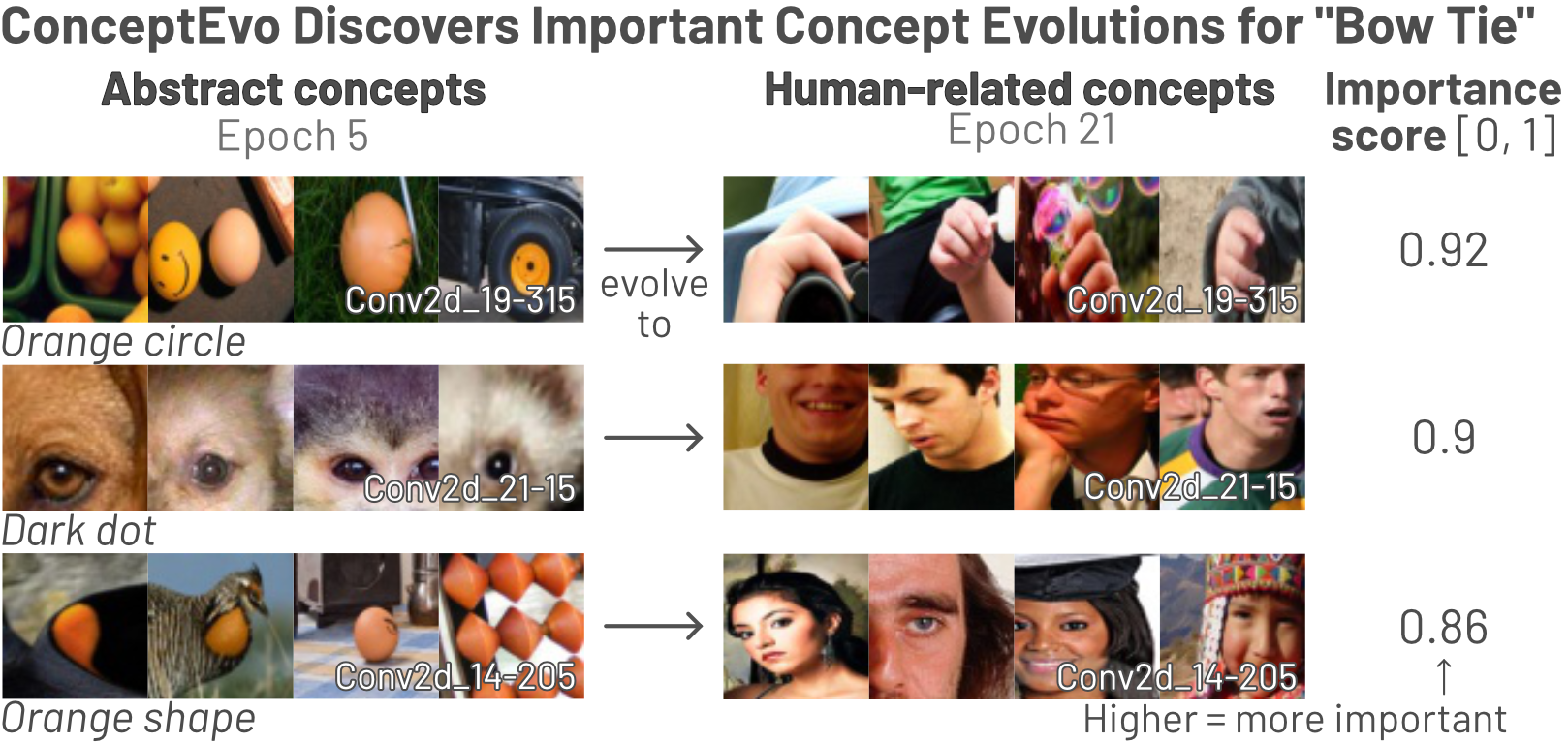
Figure 3. ConceptEvo identifies and quantifies important concept evolutions for class prediction. For example, in a VGG16, it discovers that concepts evolving towards human-related attributes, such as “orange circles” $\rightarrow$ “hand” in the top row, are important for the “bow tie” class. The importance score for this evolution is 0.92, meaning that such a concept evolution enhances predictions for 92% of bow tie images.

3.4. Runtime and Time Complexity

We designed ConceptEvo with a focus on practicality, considering the need for real-time interpretation during model training. To ensure this, we aimed to keep the runtime of our approach shorter than a single training epoch, allowing simultaneous training and interpretation. Our approach meets this requirement. Below, we report the runtime of ConceptEvo when using an NVIDIA A6000 GPU with 40GB RAM and the 10% randomly sampled ImageNet dataset (Russakovsky et al., 2015) with 120 K images.

In the two-step concept evolution interpretation method of ConceptEvo (described in Sec. 3.2), Step 1, which creates the base semantic space, completes in less than 30 minutes. Step 2, which unifies the semantic space of models across epochs, takes less than 3 hours for Step 2.1 (image embedding) and less than 1 hour for Step 2.2 (identifying stimuli of a non-base model and approximating the embedding of its neurons).

Step 2.2 ($\sim$1 hour) is the only procedure that needs to be performed when projecting concepts in a new model onto the unified semantic space, and its runtime is shorter than training a model for an epoch (e.g., ConvNeXt takes 1.56 hours). This means that ConceptEvo’s interpretation can be performed concurrently with model training. Step 1 ($\sim$30 minutes) and Step 2.1 ($\sim$3 hours) are one-time computations that can be reused, making ConceptEvo a practical and efficient choice.

3.4.1. General Interpretation of Concept Evolution (Sec. 3.2)

Now, we provide a detailed analysis of the time complexity of ConceptEvo’s two-step concept evolution interpretation method described in Section 3.2. The “steps” mentioned here correspond to the steps outlined in Section 3.2.

Step 1: Creating the base semantic space. Step 1 has an overall time complexity of $O(|N_{M_{b}}|\cdot|I|)$, where $N_{M_{b}}$ is the set of neurons in $M_{b}$, and $I$ is the set of images.

In Step 1.1, the time complexity is $O(|N_{M_{b}}|\cdot|I|)$. For each neuron, collecting the top $k$ images from $|I|$ images takes $O(|I|\cdot k)$. This process involves maintaining a sorted list of length $k$, which stores the top-$k$ images observed so far. At each iteration for an image $\mathbf{x}$, we compare $\mathbf{x}$ to the smallest top-$k$ item in the list. If $\mathbf{x}$ results in a higher activation for the neuron, we insert $\mathbf{x}$ into the list and remove the previous smallest top-$k$ item. Identifying the proper spot to insert $\mathbf{x}$ and inserting it (if necessary) takes $O(k)$, and $k$ is small (e.g., 10). Thus, the total time for collecting the top $k$ images from $|I|$ images is $O(|I|\cdot k)=O(|I|)$. Therefore, for all neurons, Step 1.1 has a time complexity of $O(|N_{M_{b}}|\cdot|I|)$.

In Step 1.2, the time complexity is $O(|N_{M_{b}}|)$. Step 1.2 consists of two sub steps. First, for each image $\mathbf{x}$, collecting neurons with $\mathbf{x}$ in their stimuli takes $O(|N_{M_{b}}|)$, as it requires iterating through all stimuli of all neurons, which is a total of $O(k\cdot|N_{M_{b}}|)$. Second, for each image $\mathbf{x}$ and its corresponding co-activated neurons, sampling neuron pairs from the list of co-activated neurons with the sliding window takes $O(k\cdot|N_{M_{b}}|)=O(|N_{M_{b}}|)$. This results in $O(|N_{M_{b}}|)$ pairs of neurons. The sampling process is repeated $E$ times, thus the total time for Step 1.2 is $O(E\cdot(|N_{M_{b}}|+|N_{M_{b}}|))=O(|N_{M_{b}}|)$.

Step 1.3 takes $O(|N_{M_{b}}|)$, as the number of generated neuron pairs in Step 1.2 is $O(|N_{M_{b}}|)$. One epoch of gradient descent in Step 1.3 takes $O(|N_{M_{b}}|\cdot R)=O(|N_{M_{b}}|)$ , resulting in a final time complexity of $O(|N_{M_{b}}|)$.

Overall, the time complexity of Step 1 is $O(|N_{M_{b}}|\cdot|I|)$ + $O(|N_{M_{b}}|)+O(|N_{M_{b}}|)$ = $O(|N_{M_{b}}|\cdot|I|)$. One advantage of this approach is its linear time complexity with respect to the number of neurons, instead of quadratic time. This is because it avoids the need to compare and represent concepts for all pairs of neurons, and instead focuses on sampled pairs of neurons.

Step 2: Unifying the semantic space. Overall, Step 2 has a time complexity of $O(|N_{M_{b}}|\cdot|I|)$. In Step 2.1, the time complexity is $O(|N_{M_{b}}|\cdot|I|)$. This is because optimizing $J_{2}$ takes $O(|I|)$ time to learn $O(|I|)$ vectors, and approximately representing images not covered by the base model’s stimuli also takes $O(|N_{M_{b}}|\cdot|I|)$, similar to Step 1 (since it adapts Step 1). To represent the concepts of neurons in a non-base model $M$ within the unified semantic space, Step 2.2 takes $O(|N_{M}|\cdot|I|)$. This step involves computing stimuli for each neuron in $M$, where $N_{M}$ is the neurons in $M$, using a similar approach as in Step 1.1.

3.4.2. Concept Evolution Important for a Class (Sec. 3.3)

Finding important concept evolutions for each class $c$ requires $O(|I|\cdot|N_{M_{b}}|)$ time, since the computation of neuron sensitivity (Eq (8)) relies on the number of images labeled as $c$ (which is $O(|I|)$). In terms of runtime, on average, this process took 37 minutes for VGG16, InceptionV3, and ConvNeXt models.

4. Experiment

We evaluate how well ConceptEvo satisfies the desired properties for interpreting concept evolution (Sec 3.1, D1-3) by addressing the following research questions:

1. Alignment. How effectively does ConceptEvo align concepts of different models at different training stages in the unified semantic space? (Sec 4.2, for D1)

2. Meaningfulness. To what extent are the discovered concept evolutions semantically meaningful? (Sec 4.3, for D1)

3. Importance. How important are the discovered concept evolutions in terms of their impact on class prediction? (Sec 4.4, for D2)

4. Discoveries. How does ConceptEvo contribute to the discovery of insightful findings? (Sec 4.5, for D3)

4.1. Experiment Settings

Datasets and models. We examine concept evolutions in representative image classifiers trained on ILSVRC2012 (ImageNet) (Russakovsky et al., 2015). The models we investigate include a modern model, such as ConvNeXt (Liu et al., 2022) which draws inspiration from recent architectures such as ResNet (Targ et al., 2016), ResNeXt (Xie et al., 2017), and vision transformers (Liu et al., 2021; Kolesnikov et al., 2021). Additionally, we investigate classic models such as VGG16 (Simonyan and Zisserman, 2015), VGG19 (Simonyan and Zisserman, 2015), VGG16 without dropout layers (Srivastava et al., 2014), and InceptionV3 (Szegedy et al., 2016). To ensure comparable accuracies, we trained these models using the hyperparameters reported in prior work (Simonyan and Zisserman, 2015; Szegedy et al., 2016; Liu et al., 2022).

Hyperparameter settings. We selected hyperparameters to achieve the overarching goal of a unified semantic space that balances strong coherence among neighboring neurons with computation efficiency. Specifically, the following hyperparameters were tested within the indicated ranges: the number of stimuli per neuron ($k$) was tested from 5 to 30, with a chosen value of 10 to strike the balance; the dimension of neuron and image embeddings was set to 30 (tested from 5 to 100); the learning rate for neuron embedding was set to 0.05 and for image embedding, it was set to 0.1 (tested from 0.001 to 0.5); and the number of randomly sampled neurons per neuron pair ($R$) was set to 3 (tested from 0 to 5).

4.2. Alignment of Neuron Embeddings

To ensure the effectiveness of ConceptEvo in aligning concepts across models and epochs, we conducted a large-scale human evaluation using Amazon Mechanical Turk (MTurk), following the methodology of prior work (Park et al., 2021; Ghorbani et al., 2019). The evaluation focused on four categories: (1) hand-picked sets of neurons representing similar concepts, which served as a baseline; (2) neuron groups detected by ConceptEvo from the base model (a well-trained VGG16); (3) neuron groups in the same model at different training epochs, detected by ConceptEvo; (4) neuron groups from different models at different epochs, detected by ConceptEvo. To collect the neuron groups, we applied K-means clustering on the neuron embeddings within the unified semantic space.

We conducted concept classification tasks with 260 MTurk participants, where each participant completed nine unique tasks. Each task consisted of six neurons presented in random order, where five of them had similar concepts identified by ConceptEvo or were hand-picked, while one neuron served as a randomly selected “intruder” neuron. To help participants understand the concept of each neuron, we provided nine example image patches. Participants were not informed about the potential presence of intruders and were asked to select as many neurons as they believed to be semantically similar. They were also asked to provide a brief description of the concept they perceived. This process, as illustrated in Fig 4, essentially forms a classification task, treating the participants as classifiers and the grouped neurons as true labels. A total of 10,950 individual classification tasks were generated for the test set. From this framing, we consider success based on the level of agreement of participants with the model’s determination. Fig 5 shows an ROC curve with the participants’ determinations, demonstrating the high discernibility and alignment of ConceptEvo-detected concepts. Even when sampling concepts across different epochs and models, the AUC scores remain consistently high, ranging from 0.90 for sampling within the base model to 0.86 for sampling across different models and training epochs.

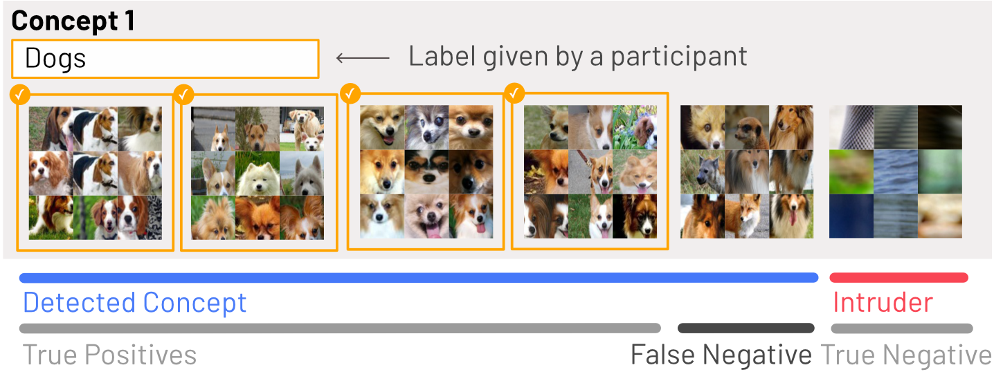
Figure 4. MTurk questionnaire example. Participants are presented with six neurons’ example patches and asked to determine if they are a semantically coherent group. If they identify a coherent group, they provide a short label for that group. In the provided example, the first five neurons are semantically similar, detected and grouped by ConceptEvo. The rightmost is randomly sampled and unrelated to others. Here, a participant correctly identifies the first four neurons as a coherent “dogs” concept (four true positives), misses the fifth neuron (one false negative), and correctly identifies the intruder as unrelated (one true negative).

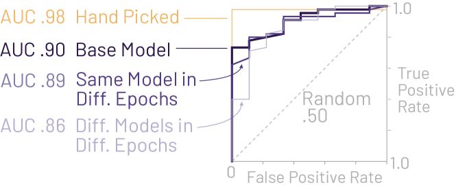
Figure 5. ROC Curve for human estimations demonstrating the high alignability of concepts discovered by ConceptEvo, even when sampled across different models and epochs.

4.3. Meaningfulness of Concept Evolution

Concepts discovered by ConceptEvo should be meaningful and informative to humans. We evaluate the interpretive consistency of the concepts labeled and described by the participants, as shown in Fig 4. To handle variations in phrasing for the labels, we use sentence-level embeddings from the Universal Sentence Encoder (USE) (Cer et al., 2018). USE captures the semantic similarity between phrases, such as “vehicle wheels,” “cars,” and “trucks”, which should have high USE similarity. To establish a baseline for similarity, we calculate the average pairwise similarity between all labels, resulting in a value of 0.28. Subsequently, we measure the average pairwise similarity between the labels provided by participants for individual concepts within each category from 4.2. The results are as follows: (1) the average concept similarity for hand-picked concepts is 0.455, (2) the average concept similarity for concepts from the base model is 0.40, (3) the average concept similarity for concepts within the same model but different epoch is 0.40, and (4) the average concept similarity for concepts from different models and different epochs is 0.38. All of these values significantly exceed the baseline similarity value of 0.28. This indicates that the concepts discovered through ConceptEvo are reliable and meaningful, even when assessed by different people.

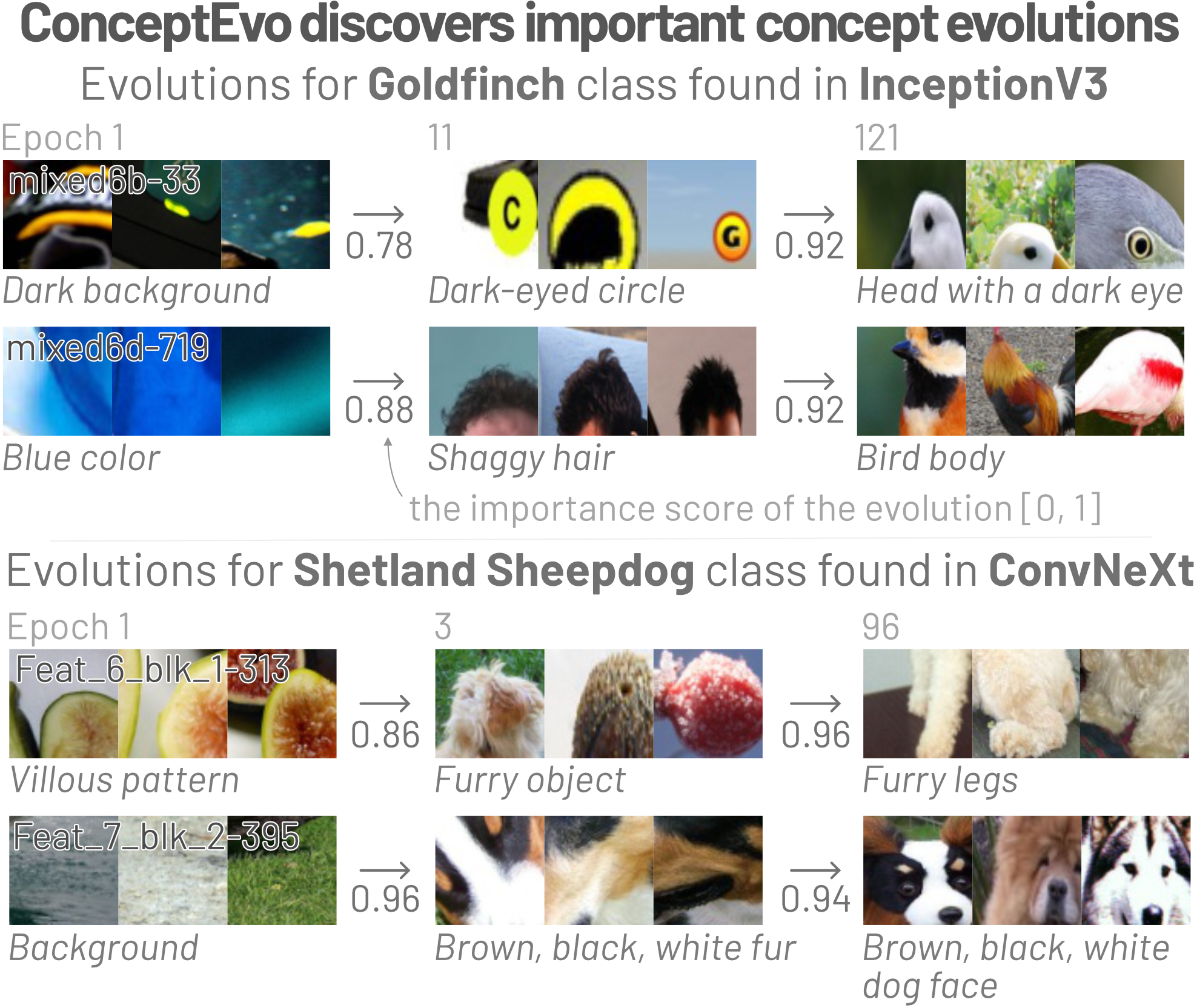
Figure 6. ConceptEvo discovers concept evolutions important for class predictions. For example, it discovers bird-related evolutions important for the “Goldfinch” class in InceptionV3, and dog-related evolutions important for the “Shetland sheepdog” class in ConvNeXt. Some neurons become increasingly specialized as training progresses. For example, in the first row, a neuron that initially detects abstract concept of dark background evolves to detect dark-eyed circle, and then further evolves to detect head with a dark eye.

4.4. Concept Evolutions Important to a Class

ConceptEvo quantifies and identifies important concept evolutions, as illustrated in Fig 6. In InceptionV3, it reveals evolutions from abstract concepts to bird-related concepts that aid in classifying the “Goldfinch” class. Similarly, in ConvNeXt, it discovers evolutions from abstract concepts to dog-related concepts that are important for classifying the “Shetland sheepdog” class. As training progresses, some neurons become more specialized. For example, in the first row of Fig 6, a neuron initially detecting abstract concepts of a dark background evolves to detect a dark-eyed circle and later to detect a head with a dark eye.

To evaluate the effectiveness of ConceptEvo in discovering important concept evolutions, we measure the changes in accuracy when evolutions are reverted, similar to how prior work evaluated concept importance in fully-trained models (Ghorbani and Zou, 2020; Ghorbani et al., 2019). By reverting a neuron’s activation map from $t^{\prime}$ to $t$, we evaluate the prediction accuracy at $t^{\prime}$. A larger drop in accuracy indicates a higher importance for the concept evolution of that neuron. To determine the stages of evolution to evaluate, we identify the epochs with the closest top-1 training accuracies to the milestones of 25%, 50%, and 75%. Specifically, for VGG16, the evolution stages are 5$\rightarrow$21 and 21$\rightarrow$207; for InceptionV3, 1$\rightarrow$11 and 11$\rightarrow$121; and for ConvNeXt, 1$\rightarrow$3 and 3$\rightarrow$96.

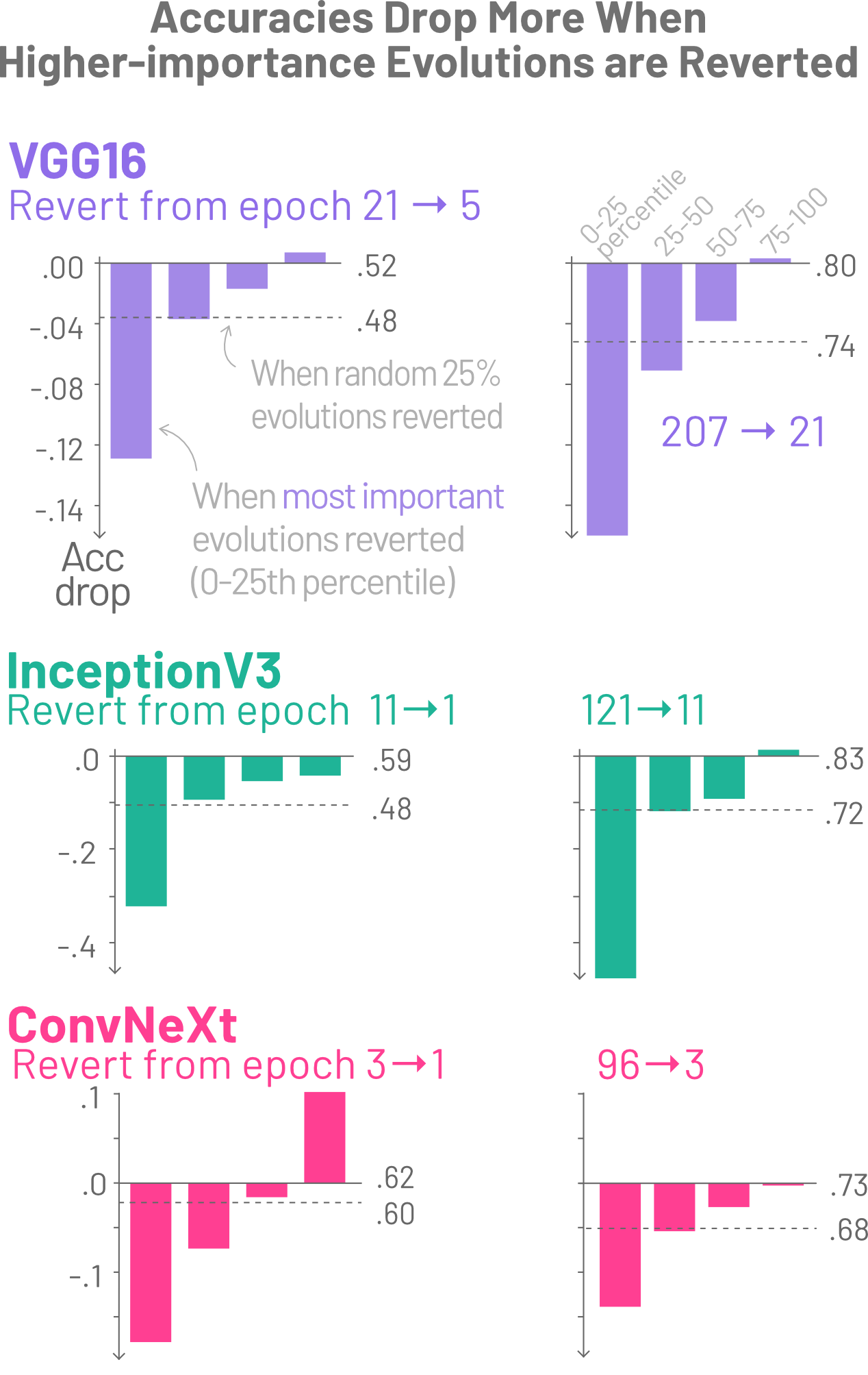
Figure 7. We evaluate the ability of ConceptEvo to quantify and identify important concept evolutions for 100 randomly selected classes. Neurons are ranked based on their evolution importance and then divided into four bins: 0-25th (most important), 25-50th, 50-75th, 75-100th percentiles. By reverting higher-importance evolutions, we observed a larger drop in top-1 training accuracy, demonstrating the effectiveness of ConceptEvo in quantifying and identifying important concept evolutions. As a baseline, for comparison, we also measured the accuracy drop when randomly reverting 25% (i.e., the same number of neurons in each bin) evolutions, which fell between the 25-50th and 50-75th percentile bins.

As ConceptEvo measures the importance of concept evolution for a single neuron (as defined in Eq 9), it is natural to evaluate accuracy changes by reverting each neuron’s evolution individually and then aggregating the changes. However, due to the large number of neurons, this approach becomes computationally prohibitive. To address this, we propose a more practical approach that reverts multiple evolutions in a layer at a time and aggregates the accuracy changes across layers. The evaluation process consists of five steps for each class $c$ and evolution stage from epoch $t$ to $t^{\prime}$. Step 1: Sample 128 images for class $c$, which corresponds to approximately 10% of the total images for that class (around 1300 images). Step 2: Compute the importance of concept evolutions for all neurons, using Eq (9). Step 3: Rank the neurons in each layer based on their evolution importance and divide them into four importance bins: 0-25th percentile (most important), 25-50th percentile, 50-75th percentile, and 75-100th percentile. Step 4: Revert the evolutions of neurons in each bin, compute the accuracy at epoch $t^{\prime}$, and measure the accuracy changes compared to the non-reverted accuracy. Step 5: Average the accuracy changes across layers to obtain the accuracy changes for the four bins. To mitigate sampling bias in Step 1, we repeat the above procedure five times independently. We average the accuracy changes across 100 randomly selected classes from the 1,000 classes in ImageNet.

Fig 7 illustrates the impact of reverting evolutions in different importance bins on the top-1 training accuracy of VGG16, InceptionV3, and ConvNeXt. Notably, reverting higher-importance evolutions (lower percentiles) results in larger accuracy drops, confirming the effectiveness of ConceptEvo in quantifying and identifying important concept evolutions. Interestingly, reverting the least important evolutions (75-100th percentile) sometimes leads to increased accuracy. This suggests that the least important evolutions may interfere with the corresponding class predictions. As a baseline, we reverted 25% randomly selected evolutions, resulting in an accuracy drop between the 25-50th percentile and the 50-75th percentile. Furthermore, we evaluated the changes in the top-5 training, top-1 test, and top-5 test accuracies when reverting evolutions in the same four bins, reinforcing our key finding that reverting higher-importance evolutions results in a larger accuracy drop.

4.5. Discovery

Incompatible hyperparameters harm concept diversity. ConceptEvo’s aligned neuron concept embedding helps identify problems caused by incompatible hyperparameters and offer insights into their impact on model performance. For example, in Fig 2b, ConceptEvo reveals that a VGG16 suboptimally trained with an excessively high learning rate exhibits a drastic accuracy drop over training epochs. Early signs of problems, such as the “atrophying” of neuron concepts that degrade concept diversity and only detect lower-level concepts, become apparent even before the accuracy reaches 0. The loss of diversity is so severe that it cannot be recovered even with 40 additional training epochs. A similar pattern is observed in a ConvNeXt model trained with a high learning rate, as shown in Fig 9a. In cases where the accuracy is low in VGG16 and ConvNeXt, we observe a significant reduction in concept diversity, especially in the last convolutional layers. For example, as seen in Fig 8, almost all neurons in VGG16 and over 30% of neurons in ConvNeXt predominantly detect “background” concepts.

In the case of an InceptionV3 unstably trained with a large learning rate, ConceptEvo reveals a similar yet slightly different scenario. As depicted in Fig 9b, the accuracy significantly drops at epoch 70, but interestingly, it recovers after a few more epochs. This recovery is likely due to the persistence of a large number of concepts at epoch 70 and the increasing diversity of concepts, despite the low accuracy.

These examples demonstrate that ConceptEvo can provide actionable insights to determine whether interventions, such as stopping the training, might be beneficial. Severe damage to concept diversity, as observed in Fig 2b and 9a, suggests that stopping the training might be more beneficial, as the model is unlikely to recover even with further epochs, compared to a better ability to recover the concept diversity as depicted in Fig 9b.

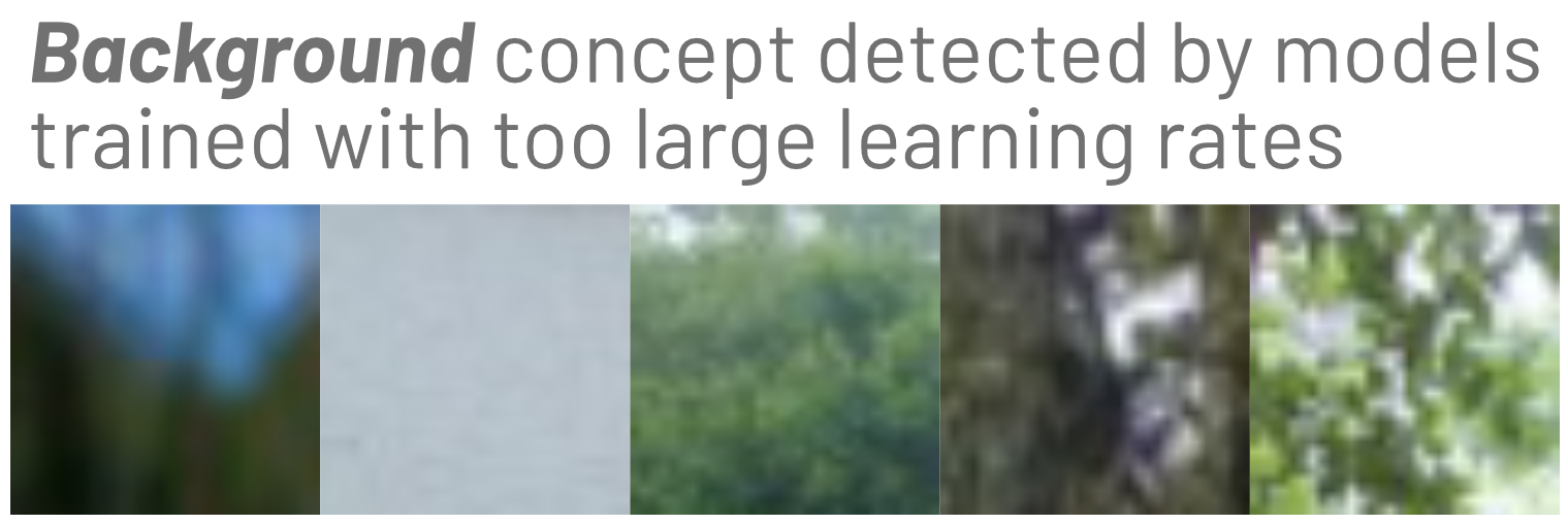
Figure 8. An example of “background” concept detected by VGG16 and ConvNeXt that are trained with overly large learning rates, when the accuracy is very low. In the last convolutional layer in these models, a notable percentage (over 30%) of neurons show exclusive intense activation in response to backgrounds of images.

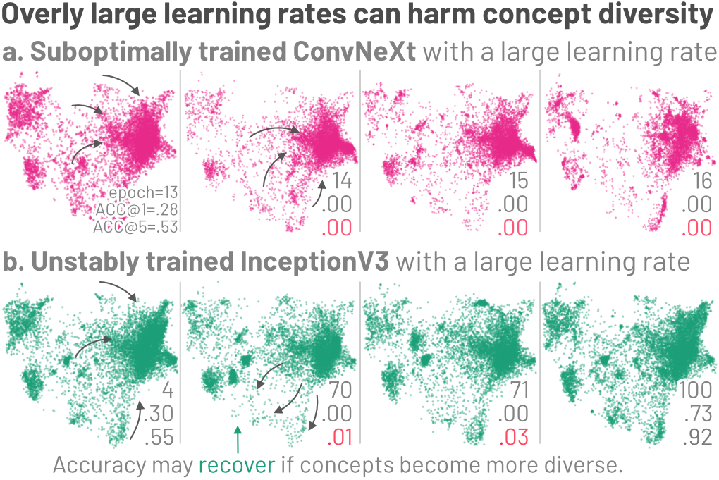
Figure 9. A suboptimally trained ConvNeXt and an unstably trained InceptionV3 with large learning rate experience decreased concept diversity and convergence in certain regions (e.g., right side to detect lower-level concepts), specifically when these models’ training accuracies drop (as seen in the second column). Interestingly, the training accuracy of InceptionV3 recovers, because the concepts become more diverse starting from epoch 70, showing a better recovery resilience.

To quantitatively study concept diversity, we use differential entropy which measures the uncertainty in a continuous variable (Michalowicz et al., 2013). We compute the differential entropy for each dimension of neuron embeddings and average the values across the dimensions. Higher values indicate more diverse concepts. In a VGG16 suboptimally trained with a large learning rate (Fig 2b), the differential entropy decreases: 1.89$\rightarrow$1.48$\rightarrow$-1.80$\rightarrow$-1.80 for epochs 3, 12, 13, 14, indicating a loss of concept diversity. Similarly, in a suboptimally trained ConvNeXt (Fig 9a), the differential entropy decreases: 1.83$\rightarrow$1.64$\rightarrow$1.59$\rightarrow$1.52 for epochs 13, 14, 15, 16. In contrast, optimally trained models show increasing differential entropy, indicating that concepts become more diverse over epochs. For example, in an optimally trained VGG16 (Fig 2a), the differential entropy increases: 1.10$\rightarrow$1.90$\rightarrow$2.06$\rightarrow$2.09 for epochs 0, 5, 21, 207. In the case of an unstably trained InceptionV3 (Fig 9b), the differential entropy decreases until epoch 70 (lowest accuracy) and then rebounds: 1.82$\rightarrow$1.32$\rightarrow$1.54$\rightarrow$1.80 for epochs 4, 70, 71, 100, indicating that its concept diversity was initially damaged but later restored.

Overfitting slows concept evolution. Overfitting is a common issue in DNN training (Rice et al., 2020; Cogswell et al., 2016). Using ConceptEvo, we have discovered that concepts in overfitted models evolve at a slower pace, despite experiencing rapid increases in training accuracy. To intentionally induce overfitting, we modified a VGG16 (Fig 2c) by removing its dropout layers which are known to help mitigate overfitting (Srivastava et al., 2014). Additionally, we overfit a ConvNeXt model by setting the weight decay of the AdamW optimizer to 0, reducing its regularization effect (Loshchilov and Hutter, 2017). These models are overfitted expectedly.

We observed that overfitted models show slower concept evolution compared to their corresponding well-trained models. To increase the top-1 training accuracy from approximately 0.25 to 0.5 and from approximately 0.5 to 0.75, the neuron embeddings in a well-trained VGG16 model (Fig 2a) move an average Euclidean distance of 2.08e-4 and 2.90e-4, respectively. In contrast, the overfitted VGG16 model (Fig 2b) exhibits much slower movement, with neuron embeddings only shifting by 1.94e-4 and 1.76e-4 for the same accuracy increments. Similarly, for the well-trained ConvNeXt model, raising the top-1 training accuracy from approximately 0.25 to 0.5 and from approximately 0.5 to 0.75 corresponds to neuron embeddings moving an average distance of 1.49e-4 and 1.33e-4, respectively. Conversely, the overfitted ConvNeXt model shows slower movement, with neuron embeddings shifting by only 1.48e-4 and 1.27e-4 for the same accuracy increments.

4.6. Comparison with Existing Approaches

We compare ConceptEvo with existing methods for representing evolving concepts. Existing methods are not optimized to capture changes across epochs; they can only be applied to one epoch at a time, independently of other epochs. In our comparison, we consider NeuroCartography (Park et al., 2021) and ACE (Ghorbani et al., 2019). ACE represents concepts using image segments that activate a layer. We use the final layer to follow the approach described in the original work. For image segments, we use the Broden dataset (Bau et al., 2017). For 2D visualization of concepts, we use UMAP (McInnes et al., 2018). To ensure alignment across epochs, we run UMAP for all epochs simultaneously, avoiding misalignment caused by independent epoch-based reduction.

The results show that ConceptEvo effectively aligns concepts across epochs, while existing methods exhibit misalignment. In Fig 10a, the “car-related” concept neurons consistently appear at the bottom in epochs 2, 5, and 207. In contrast, Fig 10b demonstrates that the “car-related” neurons represented by NeuroCartography exhibit flipping, rotation, and shifting across epochs. Similarly, Fig 10c shows that the “car-related” image segments represented by ACE exhibit significant shifting as the concept space changes during training.

Figure 10. We compare the representation of concepts in VGG16 using ConceptEvo with existing methods. (a) The results show that ConceptEvo effectively aligns learned concepts across training epochs, by projecting similar concepts to similar embedding locations. (b) In contrast, concepts represented by NeuroCartography exhibit flipping, rotation, and shifting across epochs, indicating misalignment. (c) Similarly, concepts represented by ACE undergo significant shifting, as the entire concept space (layer activation space) changes during training, indicating misalignment as well.

5. Conclusion and Future Work

ConceptEvo is a unified interpretation framework for DNNs that reveals the inception and evolution of detected concepts during training. Through both large-scale human experiments and quantitative analyses, we have showcased the effectiveness of ConceptEvo in discovering concept evolutions that facilitate human interpretation of model training across different models. This framework not only aids in identifying potential training problems but also provides guidance for interventions to achieve more stable and effective training outcomes.

In our future work, we plan to expand the scope of our investigation to include other types of models, such as object detectors, reinforcement learning systems, and language models. Additionally, we aim to enhance the alignment of concepts across different models during training. Currently, our framework operates under the assumption that an image can be represented by linear combinations of various neurons. However, more complex relationships may exist beyond linear associations. Thus, we aspire to improve the concept alignment by considering these non-linear relationships, enabling a more comprehensive and accurate representation of concepts across different models.

6. Acknowledgments

This work was supported in part by Cisco, DARPA GARD, J.P. Morgan PhD Fellowship, NSF #2144194, gifts from Amazon, Avast, Fiddler Labs, Bosch, Facebook, Intel, NVIDIA, Google, Symantec.

References

- (1)
- Abadi et al. (2016) Martín Abadi, Paul Barham, Jianmin Chen, Zhifeng Chen, Andy Davis, Jeffrey Dean, Matthieu Devin, Sanjay Ghemawat, Geoffrey Irving, Michael Isard, et al. 2016. TensorFlow: A System for Large-Scale Machine Learning. , 265–283 pages.
- Arora et al. (2019) Sanjeev Arora, Nadav Cohen, Noah Golowich, and Wei Hu. 2019. A convergence analysis of gradient descent for deep linear neural networks. International Conference on Learning Representations (ICLR) (2019).
- Bau et al. (2017) David Bau, Bolei Zhou, Aditya Khosla, Aude Oliva, and Antonio Torralba. 2017. Network dissection: Quantifying interpretability of deep visual representations. Proceedings of the IEEE conference on computer vision and pattern recognition (2017), 6541–6549.
- Cer et al. (2018) Daniel Cer, Yinfei Yang, Sheng-yi Kong, Nan Hua, Nicole Limtiaco, Rhomni St John, Noah Constant, Mario Guajardo-Cespedes, Steve Yuan, Chris Tar, et al. 2018. Universal sentence encoder for English. In Proceedings of the 2018 conference on empirical methods in natural language processing: system demonstrations. 169–174.
- Chen et al. (2019) Chaofan Chen, Oscar Li, Daniel Tao, Alina Barnett, Cynthia Rudin, and Jonathan K Su. 2019. This looks like that: deep learning for interpretable image recognition. Advances in neural information processing systems 32 (2019).
- Chung et al. (2016) Sunghyo Chung, Cheonbok Park, Sangho Suh, Kyeongpil Kang, Jaegul Choo, and Bum Chul Kwon. 2016. ReVACNN: Steering convolutional neural network via real-time visual analytics. In Future of interactive learning machines workshop at the 30th annual conference on neural information processing systems (NIPS).
- Cogswell et al. (2016) Michael Cogswell, Faruk Ahmed, Ross Girshick, Larry Zitnick, and Dhruv Batra. 2016. Reducing overfitting in deep networks by decorrelating representations. The International Conference on Learning Representations (ICLR) (2016).
- Das et al. (2020) Nilaksh Das, Haekyu Park, Zijie J Wang, Fred Hohman, Robert Firstman, Emily Rogers, and Duen Horng Polo Chau. 2020. Bluff: Interactively Deciphering Adversarial Attacks on Deep Neural Networks. IEEE Visualization Conference (2020).
- Elsken et al. (2019) Thomas Elsken, Jan Hendrik Metzen, and Frank Hutter. 2019. Neural architecture search: A survey. The Journal of Machine Learning Research 20, 1 (2019), 1997–2017.
- Fong and Vedaldi (2018) Ruth Fong and Andrea Vedaldi. 2018. Net2Vec: Quantifying and Explaining How Concepts Are Encoded by Filters in Deep Neural Networks. In 2018 IEEE Conference on Computer Vision and Pattern Recognition, CVPR. Computer Vision Foundation / IEEE Computer Society, 8730–8738.
- Gan et al. (2015) Chuang Gan, Naiyan Wang, Yi Yang, Dit-Yan Yeung, and Alex G Hauptmann. 2015. Devnet: A deep event network for multimedia event detection and evidence recounting. In Proceedings of the IEEE Conference on Computer Vision and Pattern Recognition. 2568–2577.
- Ghorbani et al. (2019) Amirata Ghorbani, James Wexler, James Zou, and Been Kim. 2019. Towards automatic concept-based explanations. Neural Information Processing Systems (2019).
- Ghorbani and Zou (2020) Amirata Ghorbani and James Y Zou. 2020. Neuron shapley: Discovering the responsible neurons. Advances in Neural Information Processing Systems 33 (2020), 5922–5932.
- Goyal et al. (2019) Yash Goyal, Uri Shalit, and Been Kim. 2019. Explaining Classifiers with Causal Concept Effect (CaCE). CoRR abs/1907.07165 (2019).
- Guidotti et al. (2018) Riccardo Guidotti, Anna Monreale, Salvatore Ruggieri, Franco Turini, Fosca Giannotti, and Dino Pedreschi. 2018. A survey of methods for explaining black box models. ACM computing surveys (CSUR) (2018).
- Gulshad and Smeulders (2020) Sadaf Gulshad and Arnold Smeulders. 2020. Explaining with counter visual attributes and examples. In Proceedings of the 2020 international conference on multimedia retrieval. 35–43.
- Hernandez et al. (2022) Evan Hernandez, Sarah Schwettmann, David Bau, Teona Bagashvili, Antonio Torralba, and Jacob Andreas. 2022. Natural Language Descriptions of Deep Features. In International Conference on Learning Representations. https://openreview.net/forum?id=NudBMY-tzDr
- Keskar et al. (2017) Nitish Shirish Keskar, Dheevatsa Mudigere, Jorge Nocedal, Mikhail Smelyanskiy, and Ping Tak Peter Tang. 2017. On large-batch training for deep learning: Generalization gap and sharp minima. 5th International Conference on Learning Representations, ICLR (2017).
- Kim et al. (2018) Been Kim, Martin Wattenberg, Justin Gilmer, Carrie Cai, James Wexler, Fernanda Viegas, et al. 2018. Interpretability beyond feature attribution: Quantitative testing with concept activation vectors (tcav). International conference on machine learning (2018).
- Koh and Liang (2017) Pang Wei Koh and Percy Liang. 2017. Understanding black-box predictions via influence functions. International Conference on Machine Learning (2017).
- Kolesnikov et al. (2021) Alexander Kolesnikov, Alexey Dosovitskiy, Dirk Weissenborn, Georg Heigold, Jakob Uszkoreit, Lucas Beyer, Matthias Minderer, Mostafa Dehghani, Neil Houlsby, Sylvain Gelly, Thomas Unterthiner, and Xiaohua Zhai. 2021. An Image is Worth 16x16 Words: Transformers for Image Recognition at Scale.
- Laugel et al. (2019) Thibault Laugel, Marie-Jeanne Lesot, Christophe Marsala, Xavier Renard, and Marcin Detyniecki. 2019. The dangers of post-hoc interpretability: Unjustified counterfactual explanations. International Joint Conference on Artificial Intelligence (2019).
- Li et al. (2018) Hao Li, Zheng Xu, Gavin Taylor, Christoph Studer, and Tom Goldstein. 2018. Visualizing the loss landscape of neural nets. Advances in neural information processing systems 31 (2018).
- Li et al. (2020) Mingwei Li, Zhenge Zhao, and Carlos Scheidegger. 2020. Visualizing neural networks with the grand tour. Distill 5, 3 (2020), e25.
- Liu et al. (2017) Mengchen Liu, Jiaxin Shi, Kelei Cao, Jun Zhu, and Shixia Liu. 2017. Analyzing the training processes of deep generative models. IEEE transactions on visualization and computer graphics 24, 1 (2017), 77–87.
- Liu et al. (2021) Ze Liu, Yutong Lin, Yue Cao, Han Hu, Yixuan Wei, Zheng Zhang, Stephen Lin, and Baining Guo. 2021. Swin transformer: Hierarchical vision transformer using shifted windows. In Proceedings of the IEEE/CVF International Conference on Computer Vision. 10012–10022.
- Liu et al. (2022) Zhuang Liu, Hanzi Mao, Chao-Yuan Wu, Christoph Feichtenhofer, Trevor Darrell, and Saining Xie. 2022. A convnet for the 2020s. In Proceedings of the IEEE/CVF Conference on Computer Vision and Pattern Recognition. 11976–11986.
- Loshchilov and Hutter (2017) Ilya Loshchilov and Frank Hutter. 2017. Decoupled weight decay regularization. arXiv preprint arXiv:1711.05101 (2017).
- McInnes et al. (2018) Leland McInnes, John Healy, and James Melville. 2018. Umap: Uniform manifold approximation and projection for dimension reduction. arXiv preprint arXiv:1802.03426 (2018).
- Michalowicz et al. (2013) Joseph Victor Michalowicz, Jonathan M Nichols, and Frank Bucholtz. 2013. Handbook of differential entropy. Crc Press.
- Mikolov et al. (2013a) Tomas Mikolov, Kai Chen, Greg Corrado, and Jeffrey Dean. 2013a. Efficient estimation of word representations in vector space. arXiv preprint arXiv:1301.3781 (2013).
- Mikolov et al. (2013b) Tomas Mikolov, Ilya Sutskever, Kai Chen, Greg S Corrado, and Jeff Dean. 2013b. Distributed representations of words and phrases and their compositionality. Advances in neural information processing systems 26 (2013).
- Nguyen et al. (2016) Anh Mai Nguyen, Jason Yosinski, and Jeff Clune. 2016. Multifaceted Feature Visualization: Uncovering the Different Types of Features Learned By Each Neuron in Deep Neural Networks. Visualization for Deep Learning workshop at ICML (2016).
- Olah et al. (2020) Chris Olah, Nick Cammarata, Ludwig Schubert, Gabriel Goh, Michael Petrov, and Shan Carter. 2020. Zoom in: An introduction to circuits. Distill 5, 3 (2020), e00024–001.
- Olah et al. (2017) Chris Olah, Alexander Mordvintsev, and Ludwig Schubert. 2017. Feature visualization. Distill 2, 11 (2017), e7.
- Papernot and McDaniel (2018) Nicolas Papernot and Patrick McDaniel. 2018. Deep k-nearest neighbors: Towards confident, interpretable and robust deep learning. arXiv preprint arXiv:1803.04765 (2018).
- Park et al. (2021) Haekyu Park, Nilaksh Das, Rahul Duggal, Austin P Wright, Omar Shaikh, Fred Hohman, and Duen Horng Polo Chau. 2021. NeuroCartography: Scalable Automatic Visual Summarization of Concepts in Deep Neural Networks. IEEE Transactions on Visualization and Computer Graphics (2021).
- Pezzotti et al. (2017) Nicola Pezzotti, Thomas Höllt, Jan Van Gemert, Boudewijn PF Lelieveldt, Elmar Eisemann, and Anna Vilanova. 2017. Deepeyes: Progressive visual analytics for designing deep neural networks. IEEE transactions on visualization and computer graphics 24, 1 (2017), 98–108.
- Pühringer et al. (2020) Michael Pühringer, Andreas Hinterreiter, and Marc Streit. 2020. InstanceFlow: Visualizing the Evolution of Classifier Confusion at the Instance Level. In 2020 IEEE Visualization Conference (VIS). IEEE, 291–295.
- Raghu et al. (2017) Maithra Raghu, Justin Gilmer, Jason Yosinski, and Jascha Sohl-Dickstein. 2017. Svcca: Singular vector canonical correlation analysis for deep learning dynamics and interpretability. Advances in neural information processing systems 30 (2017).
- Rauber et al. (2016) Paulo E Rauber, Samuel G Fadel, Alexandre X Falcao, and Alexandru C Telea. 2016. Visualizing the hidden activity of artificial neural networks. IEEE transactions on visualization and computer graphics 23, 1 (2016), 101–110.
- Reddi et al. (2019) Sashank J Reddi, Satyen Kale, and Sanjiv Kumar. 2019. On the convergence of adam and beyond. arXiv preprint arXiv:1904.09237 (2019).
- Ribeiro et al. (2016) Marco Tulio Ribeiro, Sameer Singh, and Carlos Guestrin. 2016. “Why should I trust you?” Explaining the predictions of any classifier. ACM SIGKDD international conference on knowledge discovery and data mining (2016).
- Rice et al. (2020) Leslie Rice, Eric Wong, and Zico Kolter. 2020. Overfitting in adversarially robust deep learning. In International Conference on Machine Learning. PMLR, 8093–8104.
- Russakovsky et al. (2015) Olga Russakovsky, Jia Deng, Hao Su, Jonathan Krause, Sanjeev Satheesh, Sean Ma, Zhiheng Huang, Andrej Karpathy, Aditya Khosla, Michael Bernstein, et al. 2015. Imagenet large scale visual recognition challenge. International journal of computer vision 115, 3 (2015), 211–252.
- Safarik et al. (2018) Jakub Safarik, Jakub Jalowiczor, Erik Gresak, and Jan Rozhon. 2018. Genetic algorithm for automatic tuning of neural network hyperparameters. In Autonomous Systems: Sensors, Vehicles, Security, and the Internet of Everything, Vol. 10643. SPIE, 168–174.
- Selvaraju et al. (2017) Ramprasaath R Selvaraju, Michael Cogswell, Abhishek Das, Ramakrishna Vedantam, Devi Parikh, and Dhruv Batra. 2017. Grad-cam: Visual explanations from deep networks via gradient-based localization. IEEE international conference on computer vision (2017), 618–626.
- Simonyan et al. (2013) Karen Simonyan, Andrea Vedaldi, and Andrew Zisserman. 2013. Deep inside convolutional networks: Visualising image classification models and saliency maps. arXiv preprint arXiv:1312.6034 (2013).
- Simonyan and Zisserman (2015) Karen Simonyan and Andrew Zisserman. 2015. Very Deep Convolutional Networks for Large-Scale Image Recognition. International Conference on Learning Representations (ICLR) (2015).
- Smilkov et al. (2017) Daniel Smilkov, Shan Carter, D Sculley, Fernanda B Viégas, and Martin Wattenberg. 2017. Direct-manipulation visualization of deep networks. arXiv preprint arXiv:1708.03788 (2017).
- Srivastava et al. (2014) Nitish Srivastava, Geoffrey Hinton, Alex Krizhevsky, Ilya Sutskever, and Ruslan Salakhutdinov. 2014. Dropout: a simple way to prevent neural networks from overfitting. The journal of machine learning research 15, 1 (2014), 1929–1958.
- Szegedy et al. (2016) Christian Szegedy, Vincent Vanhoucke, Sergey Ioffe, Jon Shlens, and Zbigniew Wojna. 2016. Rethinking the inception architecture for computer vision. IEEE conference on computer vision and pattern recognition (2016).
- Targ et al. (2016) Sasha Targ, Diogo Almeida, and Kevin Lyman. 2016. Resnet in resnet: Generalizing residual architectures. arXiv preprint arXiv:1603.08029 (2016).
- Xie et al. (2017) Saining Xie, Ross Girshick, Piotr Dollár, Zhuowen Tu, and Kaiming He. 2017. Aggregated residual transformations for deep neural networks. In Proceedings of the IEEE conference on computer vision and pattern recognition. 1492–1500.
- Yeh et al. (2020) Chih-Kuan Yeh, Been Kim, Sercan Ömer Arik, Chun-Liang Li, Tomas Pfister, and Pradeep Ravikumar. 2020. On Completeness-aware Concept-Based Explanations in Deep Neural Networks. In Advances in Neural Information Processing Systems 33: Annual Conference on Neural Information Processing Systems 2020, NeurIPS, Hugo Larochelle, Marc’Aurelio Ranzato, Raia Hadsell, Maria-Florina Balcan, and Hsuan-Tien Lin (Eds.).
- Yosinski et al. (2015) Jason Yosinski, Jeff Clune, Anh Nguyen, Thomas Fuchs, and Hod Lipson. 2015. Understanding neural networks through deep visualization. International Conference on Machine Learning (ICML) Deep Learning Workshop (2015).
- Zeiler and Fergus (2014) Matthew D Zeiler and Rob Fergus. 2014. Visualizing and understanding convolutional networks. In European conference on computer vision. Springer, 818–833.
- Zhang et al. (2021) Chiyuan Zhang, Samy Bengio, Moritz Hardt, Benjamin Recht, and Oriol Vinyals. 2021. Understanding deep learning (still) requires rethinking generalization. Commun. ACM 64, 3 (2021), 107–115.
- Zhang et al. (2018) Quanshi Zhang, Wenguan Wang, and Song-Chun Zhu. 2018. Examining cnn representations with respect to dataset bias. AAAI Conference on Artificial Intelligence (2018).
- Zhong et al. (2017) Wen Zhong, Cong Xie, Yuan Zhong, Yang Wang, Wei Xu, Shenghui Cheng, and Klaus Mueller. 2017. Evolutionary visual analysis of deep neural networks. In ICML Workshop on Visualization for Deep Learning. 9.
- Zhou et al. (2018) Bolei Zhou, David Bau, Aude Oliva, and Antonio Torralba. 2018. Interpreting deep visual representations via network dissection. IEEE transactions on pattern analysis and machine intelligence 41, 9 (2018), 2131–2145.
- Zhou et al. (2022) Zhiyan Zhou, Kevin Li, Haekyu Park, Megan Dass, Austin Wright, Nilaksh Das, and Duen Horng Chau. 2022. NeuroMapper: In-browser Visualizer for Neural Network Training. IEEE Visualization Conference (IEEE VIS) (2022).