Magnetic structure and properties of a vanthoffite mineral $Na_{6}Mn(SO_{4})_{4}$

Abstract

A detailed analysis of the magnetic properties of a vanthoffite type mineral $Na_{6}Mn(SO_{4})_{4}$ based on dc magnetization, low temperature neutron powder diffraction and theoretical calculations is reported. The mineral crystallizes in a monoclinic system with space group $P2_{1}/c$, where $MnO_{6}$ octahedra are linked via $SO_{4}$ tetrahedra. This gives rise to super-exchange interaction between two $Mn^{2+}$ ions mediated by two nonmagnetic bridging anions and leads to an antiferromagnetic ordering below 3 K. The magnetic structure derived from neutron powder diffraction at 1.7 K depicts an antiferromagnetic spin arrangement in the $bc$ plane of the crystal. The magnetic properties are modelled by numerical calculations using exact diagonalization technique, which fits the experimental results and provides antiferromagnetic ground state of $Na_{6}Mn(SO_{4})_{4}$.

I Introduction

Over the last two decades, design of polyanionic materials [$(XO_{4})_{n}$ with $X$ = S, P, As, V, Si, Mo or W] has attracted significant attention due to their adaptability towards various potential applications. For example, the discovery and commercialization of $LiFePO_{4}$ Padhi-JES-1997 ; Wang-EES-2015 significantly shed light on the use of insertion materials in battery research with other polyanionic units Masquelier-CR-2013 ; Melot-ACR-2013 ; Gong-EES-2011 ; Rousse-CM-2014 . In this context, it may be noted that many naturally occurring minerals with a variety of polyanionic units offer a treasure trove of materials with associated tunable properties. Moreover, the presence of $3d$ transition metals in the chemical composition of such materials will open up the possibility of synthesizing solids with interesting magnetic behaviour. Several electrode materials inspired by the naturally occurring minerals have been investigated leading to the discovery of interesting magnetic properties in these materials Reynaud-IC-2013 ; Reynaud-PRB-2014 ; Sun-CM-2015 ; Rousse-PRB-2017 ; Lander-IC-2016 ; Furrer-PRB-2020 . The coupling between magnetic and electrical properties in $3d$ metal based polyanionic compounds results in magnetoelectric effect Reynaud-PRB-2014 ; Lander-IC-2016 ; Petersen-PRB-2012 ; Li-PRB-2009 ; Dell-EP-1965 ; Fogh-PRB-2017 ; Lander-JMCA-2015 ; Scaramucci-PRL-2012 ; Kornev-PRB-2000 ; Fiebig-JPDAP-2005 ; Aken-Nature-2007 ; Bousquet-PRL-2011 , which has been successfully utilized to design various multiferroic materials Rivera-EPJB-2009 ; Rousse-PRB-2013 ; Yanda-ACPM-2020 . Specifically, the compound $TbPO_{4}$ Rado-PRB-1984 ; Bluck-JPC-1988 displays intrinsic bulk magneto-electric effect. A series of polyanionic phosphates $LiMPO_{4}$ ($M$ = Mn, Co, Ni or Fe) have aroused special interest to evaluate the associated magnetic behaviour in these minerals Kornev-PRB-2000 ; Vaknin-PRB-2002 ; Rousse-CM-2003 ; Vaknin-PRL-2004 ; Gnewuch-IC-2020 ; Fogh-PRB-2019 .

The origin of magnetic interactions in these transition metal oxides, sulfates, phosphates and arsenates are governed by the overlap between 3d orbitals of the transition metal and 2p orbitals of the oxygen atom. Usually, in super exchange interactions, two magnetic metal centers are bridged via a single electronegative anion, like oxygen (M-O-M). However, in this material two metal centers interact via two oxygen atoms (M-O-O-M) and the magnetic interactions are hence weaker. A set of semi-empirical rules referred to as Goodenough-Kanamori-Anderson rules which these systems follow, are well described in the literature Anderson-PR-1959 ; Kanamori-JPCS-1959 ; Goodenough-PR-1955 ; Goodenough-JPCS-1958 ; Goodenough-PR-1961 ; Rousse-CM-2001 .

Many polyanionic compounds have been largely studied for their structural diversity where both types of interactions (M-O-M or M-O-O-M) are possible when changing the $3d$ transition metal as well as polyanions (e.g. $PO_{4}$, $SO_{4}$, $AsO_{4}$, $VO_{4}$ etc). For example, the magnetic structure of anhydrous $FeSO_{4}$ and $NiSO_{4}$ have antiferromagnetic sheets with ferromagnetic coupling between the sheets whereas in the case of $CoSO_{4}$, only antiferromagnetic ordering exists within each sheet. But the magnetic structure of $CrVO_{4}$ has ferromagnetically ordered sheets that stack antiferromagnetically. However, in each case, magnetic coupling involves a long super exchange pathway between magnetic centers via nonmagnetic sulfate or vanadate tetrahedron Frazer-PR-1962 . Beside these class of materials, other families of electrode materials such as fluorosulfates Melot-CM-2011 ; Melot-IC-2011 ; Melot-PRB-2012 , phosphates Kornev-PRB-2000 ; Vaknin-PRB-2002 ; Rousse-CM-2003 ; Rousse-CM-2001 ; Rousse-SSS-2002 ; Rousse-APA-2002 and borates Tao-IC-2013 have been studied and these materials also exhibit magnetic ordering at low temperatures. In fluorosulfates magnetic exchange interaction between nearest-neighbour ions is mediated either through M-F-M link or through M-O-O-M interaction via the oxygen anions at the sulfate tetrahedral edge.

Materials designed for potential battery electrode applications are also recognized as model compounds for their intriguing magnetic property; examples are marinate phases $Li_{2}M(SO_{4})_{2}$ ($M$ = Mn, Fe or Co) and $LiFe(SO_{4})_{2}$ Reynaud-IC-2013 . At low temperatures, these compounds show antiferromagnetic ordering due to a specific arrangement of transition metal octahedra ($MO_{6}$) and sulphate tetrahedra ($SO_{4}$). This particular structural arrangement solely enables the M-O-O-M exchange pathway between transition metal ions. Another interesting example in this series is the orthorhombic $Li_{2}Ni(SO_{4})_{2}$ reported by Reynaud et al Reynaud-PRB-2014 . It has a particular arrangement of isolated $NiO_{6}$ octahedra which are interconnected via $SO_{4}$ tetrahedral units. As a result of exchange interaction between the $3d$ transition metal cations via two bridging ions, this phase is antiferromagnetic with a $T_{N}$= 28 K. Similar long-range antiferromagnetic ordering is also observed with isostructural orthorhombic $Li_{2}M(SO_{4})_{2}$ ($M$ = Mn, Fe or Co) phase Lander-IC-2016 .

It is of interest to note that, Vanthoffite minerals occur in nature as oceanic salt deposits Keester-ACSB-1977 ; Dutta-IC-2020 . We have shown earlier that the crystal structure of $Na_{6}Mn(SO_{4})_{4}$(a Vanthoffite mineral) is built from an alternating corner-sharing of $SO_{4}$ tetrahedra and transition metal octahedra $MnO_{6}$ resulting in an infinite two-dimensional framework in the $bc$ plane Sharma-IC-2017 . Such specific connectivity suggests the possibility of long exchange pathway between two $Mn^{2+}$ centers via two oxygen atoms (Mn-O-O-Mn), which might lead to magnetic interaction akin to several other examples reported in the literature Reynaud-IC-2013 ; Reynaud-PRB-2014 ; Lander-IC-2016 . In this article, we investigate the magnetic structure of $Na_{6}Mn(SO_{4})_{4}$ using variable temperature neutron diffraction. Besides, we have carried out exact diagonalization calculations of the model Hamiltonian to shed light on the magnetic properties and magnetic structure.

II Experimental Method

Single crystals of $Na_{6}Mn(SO_{4})_{4}$ were grown by slow evaporation at 80^∘C from an aqueous solution containing 3:1 stoichiometric molar ratio of $Na_{2}SO_{4}$ (Sigma-Aldrich, 99.99%) and $MnSO_{4}.H_{2}O$ (Sigma-Aldrich, 99.99%) as described in the earlier publication Sharma-IC-2017 . Colourless block-shaped crystals were obtained after 15 days. The single crystal x-ray diffraction of the as grown crystal was carried out on an Oxford Xcalibur(Mova) diffractometer equipped with an EOS CCD detector and a microfocus sealed tube using MoK$\alpha$ X-radiation ($\lambda$ = 0.71073 Å; 50 kV and 0.8 mA) and the structural parameters agree with the earlier report Sharma-IC-2017 . Single crystals were crushed to form bulk polycrystalline powder for further characterization. Room temperature PXRD data was recorded on a PANalytical X’Pert PRO diffractometer using Cu K$\alpha$ range of 8-60^∘ using a step size of 0.013^∘. X’Pert High Score Plus (version 4.8) Degen-PD-2014 was used to analyze the pattern and profile fitting refinements were carried out using the room temperature unit cell parameters of $Na_{6}Mn(SO_{4})_{4}$ Sharma-IC-2017 in JANA2006 Petricek-ZKM-2014 . Profile parameters such as GU, GV, GW, LX, and LY were refined using Pseudo-Voigt function. Neutron diffraction patterns over a wide $Q$-range ($4\pi sin\theta/\lambda=0.3-9.5$Å^-1 where $2\theta$ and $\lambda$ are the scattering angle and wavelength of the incident neutron beam, respectively) were recorded over 1.7-300 K by using the powder diffractometer PD-II ($\lambda$ = 1.2443 Å) at Dhruva reactor, Trombay, INDIA Siruguri-NN-2000 . For the neutron diffraction measurements, the powder sample was filled in a vanadium can of diameter 6 mm. All the low-temperature measurements were performed by using a closed-cycle helium refrigerator. The neutron diffraction patterns were analyzed by Rietveld refinement method using the FULLPROF suite program Carvajal-PB ; Bera-JPCC-2020 ; Bera-MRE-2015 ; Bera-SSS-2013 ; Saha-SSC-2011 . Temperature and magnetic field-dependent dc-susceptibility measurements were probed with a commercial vibrating sample magnetometer (Cryogenic Co. Ltd., UK). The temperature-dependent magnetization curves [$M$ vs. $T$] were recorded in the warming cycles over the temperature range of 2-300 K in both zero-field-cooled (ZFC) and field-cooled (FC) conditions. Isothermal magnetization curve was measured at 2 K in the increasing and decreasing field cycles up to 90 kOe.

Figure 1: (a) Packing diagram of $Na_{6}Mn(SO_{4})_{4}$ viewed down the $c$-axis, (b) Highlighting the connectivity between $MnO_{6}$ and $SO_{4}$ tetrahedra, (c) Packing diagram viewed down $a$-axis, sodium atoms are removed for the clarity of the picture, (d) Mn-O-O-Mn interaction pathway through $MnO_{6}$ octahedra and $SO_{4}$ tetrahedra, and (e) Arrangement of Mn sublattice in the structure showing the nearest neighbours (red bonds) and next-nearest neighbours (blue bonds).

Figure 2: Le Bail profile refinement of $Na_{6}Mn(SO_{4})_{4}$ at room temperature.

III RESULTS AND DISCUSSION

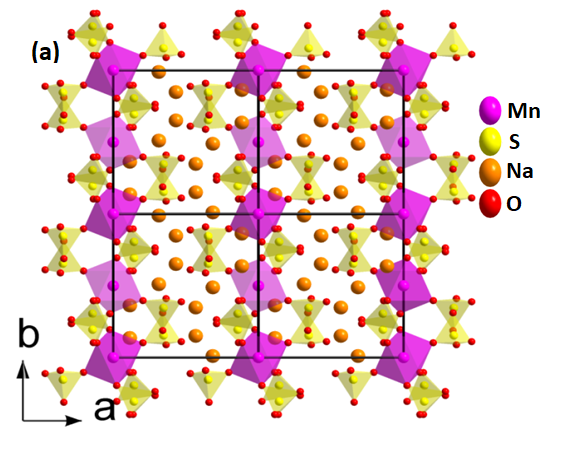
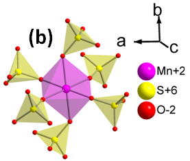
$Na_{6}Mn(SO_{4})_{4}$ belongs to a monoclinic system, space group $P2_{1}/c$ with Z = 2 as determined from single crystal X-ray diffraction for the present work and agrees well with the earlier report by our group Sharma-IC-2017 . The fractional coordinates of all atoms and the bond lengths and angles for $MnO_{6}$ octahedra are given in Table 1 and 2. The asymmetric unit contains half the formula unit, where Mn atom is in a special position (Wyckoff position 2$a$, local site symmetry -1) along with three sodium atoms and two sulfate units in general position (Wyckoff position 4$e$, local site symmetry 1) [Table 1]. Mn atom forms $MnO_{6}$ octahedra with symmetrically related oxygen atoms and connected to $SO_{4}$ tetrahedra in a “pinwheel pattern”. (Figure 1b) Brian-JEPM-1973 .

Table 1: Crystallographic details and fractional atomic coordinates for $Na_{6}Mn(SO_{4})_{4}$

Empirical formula = $Na_{6}Mn(SO_{4})_{4}$, Formula weight (g/mol)=577.12, Space Group = $P2_{1}/c$,
$a$= 9.7131(13) Å, $b$ = 9.2926(11) Å, $c$ = 8.2609(12) Å, $\beta$ =112.988(7)∘,
$V$ = 686.42(16) Å3, $R_{obs}[I>2\sigma(I)]$ = 0.0183, $wR_{obs}[I>2\sigma(I)]$ =0.0541
Atom	Wickoff position	Occupancy	$\mathbf{x}/a$	$\mathbf{y}/b$	$\mathbf{z}/c$	$\mathbf{u_{iso}(\AA^{2})}$	BVS
Mn1	2$a$	0.5	0.000000	0.000000	0.000000	0.01093(11)	1.927
Na1	4$e$	1	0.11489(9)	0.36352(8)	0.18562(11)	0.02590(19)	1.079
Na2	4$e$	1	0.31418(8)	-0.01160(7)	0.46824(9)	0.01645(17)	1.105
Na3	4$e$	1	0.43369(9)	-0.15142(8)	0.07766(10)	0.02486(19)	1.060
S1	4$e$	1	0.34511(4)	0.15332(4)	0.16518(5)	0.01101(12)	6.028
S2	4$e$	1	0.14234(4)	-0.30579(4)	0.21800(5)	0.01055(12)	6.060
O1	4$e$	1	0.20375(13)	0.10249(13)	0.17787(15)	0.0159(3)	2.038
O2	4$e$	1	0.33934(14)	0.31084(13)	0.15062(16)	0.0173(3)	2.134
O3	4$e$	1	0.36223(15)	0.08889(14)	0.01351(17)	0.0222(3)	2.043
O4	4$e$	1	0.46806(13)	0.11001(14)	0.32974(17)	0.0201(3)	2.110
O5	4$e$	1	0.02432(14)	-0.19349(13)	0.15358(17)	0.0176(3)	2.046
O6	4$e$	1	0.28843(14)	-0.23682(14)	0.30234(18)	0.0218(3)	1.979
O7	4$e$	1	0.13626(14)	-0.39575(13)	0.06987(16)	0.0196(3)	2.061
O8	4$e$	1	0.11064(16)	-0.39682(14)	0.34471(18)	0.0229(3)	1.983

Table 2: Bond lengths and bond angles for $Na_{6}Mn(SO_{4})_{4}$

Bond	Length (Å)	Bond	Angle (∘)	Bond	Angle (∘)
Mn1-O5x2	2.1597(12)	O5-Mn1-O1x2	96.08(5)	O5-Mn1-O8x2	90.78(5)
Mn1-O1x2	2.1706(12)	O5-Mn1-O1x2	83.92(5)	O1-Mn1-O8x2	86.42(5)
Mn1-O8x2	2.1901(13)	O5-Mn1-O8x2	89.22(5)	O1-Mn1-O8x2	93.58(5)

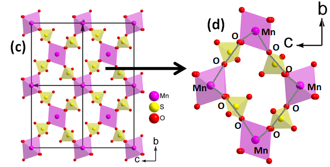
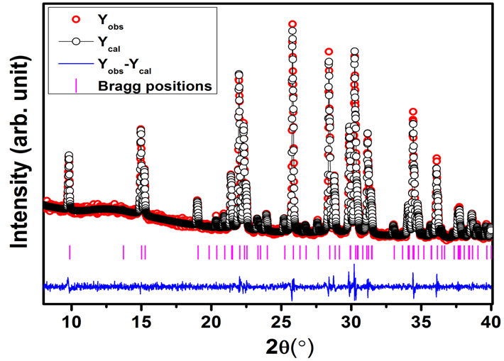
The Mn-O bond lengths in $MnO_{6}$ octahedra varies between 2.1597 (12) to 2.1901(13) Å(Table 2) where the bond length distortion parameters and bond angle variance are calculated using formulas $\Delta d=(\frac{1}{6})\sum_{n}[\frac{d_{n}-d_{av}}{d_{av}}]^{2}$ and $\sigma^{2}_{oct}=\frac{1}{11}\sum_{i}[\alpha_{i}-90]^{2}$, ($d_{n}$ and $d_{av}$ are the individual and average Mn-O bond length and $\alpha_{i}$ are the individual O-Mn-O bond angles) Lu-JACS-2020 ; Baur-ACSB ; Robinson-Science-1971 . It is to be noted that, $\Delta d$ and $\sigma_{oct}^{2}$ values for an ideal octahedron should be exactly zero. The bond length distortion parameter obtained ($\Delta d$=3.35$\times$10^-5) though indicates a quite symmetrical $MnO_{6}$ octahedra, the calculated bond angle variance of 18.32 show a distorted $MnO_{6}$ octahedra. The bond valence sum for Mn atom is calculated to be around 1.927 using the Zachariasen formula $V_{i}=\sum_{j}s_{ij}=\sum_{j}e^{\frac{d_{o}-d_{ij}}{0.37}}$ and it is in good agreement with the expected valance of +2 Brown-ACB-1985 . These are isolated $MnO_{6}$ octahedra (pink) and are connected to $SO_{4}$ tetrahedra (yellow) via their oxygen vertices (Figure 1). Thus the structure presents an exchange pathway via two bridged oxygen atoms viz., Mn-O-O-Mn magnetic interaction where Mn-O-O-Mn dihedral angle is about 148^∘ (Figure 1d). A similar long exchange pathway (M-O-O-M) is found in $Li_{2}M(SO_{4})_{2}$, ($M$ = Ni, Co, Fe, Mn), where magnetism in the materials are explained based on this interaction Reynaud-IC-2013 ; Reynaud-PRB-2014 ; Lander-IC-2016 . The single crystals grown are further crushed to form the powder sample and the phase purity was checked using PXRD measurement. The PXRD profile refinement ($R_{p}$ = 3.43, $R_{wp}$ = 4.50 and $\chi^{2}$ = 1.01) at room temperature was carried out using the cell parameter and space group obtained from the single crystal XRD, where the close similarity between the observed and the calculated patterns suggests the purity of the desired compound, $Na_{6}Mn(SO_{4})_{4}$ (Figure 2).

III.1 Magnetic Measurements

Figure 3: (a) Low temperature susceptibility curve measured under 50 Oe in ZFC mode, (b) The temperature-dependent susceptibility ($\chi$(T)) curves measured under 1000 Oe in the ZFC and FC modes. Inset shows $\chi T$ vs. $T$ plot in the ZFC mode, and (c) The inverse ZFC susceptibility as a function of temperature under 1000 Oe. The solid curve is a straight line fit to the measured data.

Figure 4: The isothermal magnetization measured at 2 K after cooling the sample in zero field. Inset shows a zoomed view in the low field region over $\pm$ 1 kOe and absence of hysteresis.

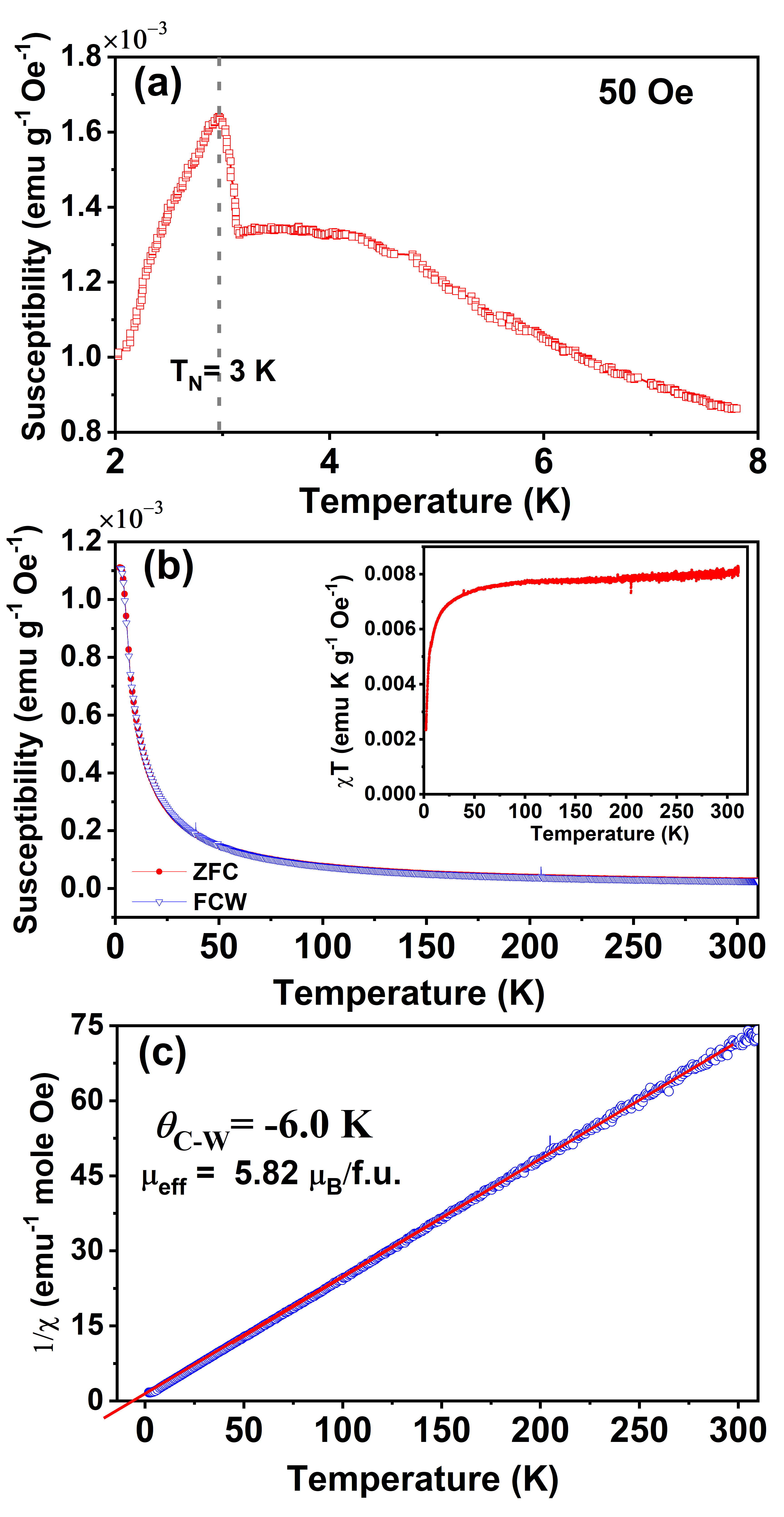
The zero-field-cooled susceptibility curve of $Na_{6}Mn(SO_{4})_{4}$ measured under magnetic field of 50 Oe (Figure 3a) shows a peak revealing a transition to antiferromagntic (AFM) state below $T_{N}$ $\sim$ 3 K. The AFM ordering is confirmed by our zero field neutron diffraction study presented later. Figure 3b shows the temperature dependent susceptibility curve measured under 1000 Oe over the temperature range 2-300 K. The $\chi$ vs T curve in Figure 3b, however does not exhibit any distinct magnetic transition in contrast to the observation made under a weak applied field of 50 Oe in Figure 3a. It is to be noted that ZFC $\chi T$ vs T plot under 1000 Oe [inset of Figure 3b] yields a downturn below 20 K. This corroborates the existing antiferromagnetic interactions in $Na_{6}Mn(SO_{4})_{4}$. We also notice that $\chi T$ value in the high temperature (paramagnetic) region increases slightly with temperature, contrary to the constant value expected in the paramagnetic region. The reason for the same could be attributed to additional contribution arising from the van Vleck paramagnetism ($\chi_{VV}$) which is discussed in the theoretical section.

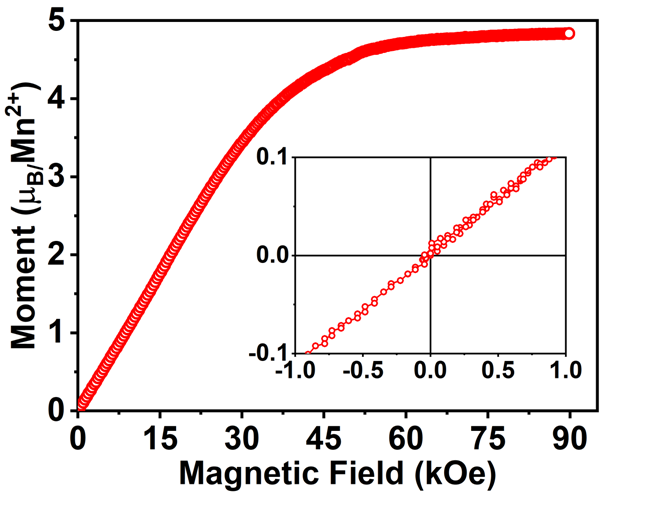
The inverse ZFC susceptibility plot under 1000 Oe is shown in Figure 3c. The linear fit to the inverse susceptibility curve yields the Curie-Weiss temperature $\Theta_{CW}$ = -6.0 K and the effective paramagnetic moment $\mu_{eff}$ = 5.8 $\mu_{B}$/f.u. The observed value of the effective moment 5.8 $\mu_{B}$/f.u is in good agreement with the theoretically expected $\mu_{eff}$ (where $\mu_{eff}(s)=g\sqrt{s(s+1)}$ with g=2 (Lande g-factor)) value of 5.92 $\mu_{B}$/Mn⁺², considering only spin moment. This result confirms +2 oxidation state of the magnetic Mn ion (s=5/2) in $Na_{6}Mn(SO_{4})_{4}$. The isothermal field dependent magnetization curve (Figure 4) measured at 2 K, shows a linear increase in the low field regime and then tends to show a change in slope above 35 kOe and a saturation above 65 kOe. However, we do not observe any opening of the hysteresis loop (inset in Figure 4) under field sweeping. The observation of negative Curie-Weiss temperature, downturn of $\chi T$ vs T, linear magnetization behaviour in the low field region and the absence of hysteresis altogether suggest an antiferromagnetic ground state of $Na_{6}Mn(SO_{4})_{4}$.

III.2 Neutron Diffraction

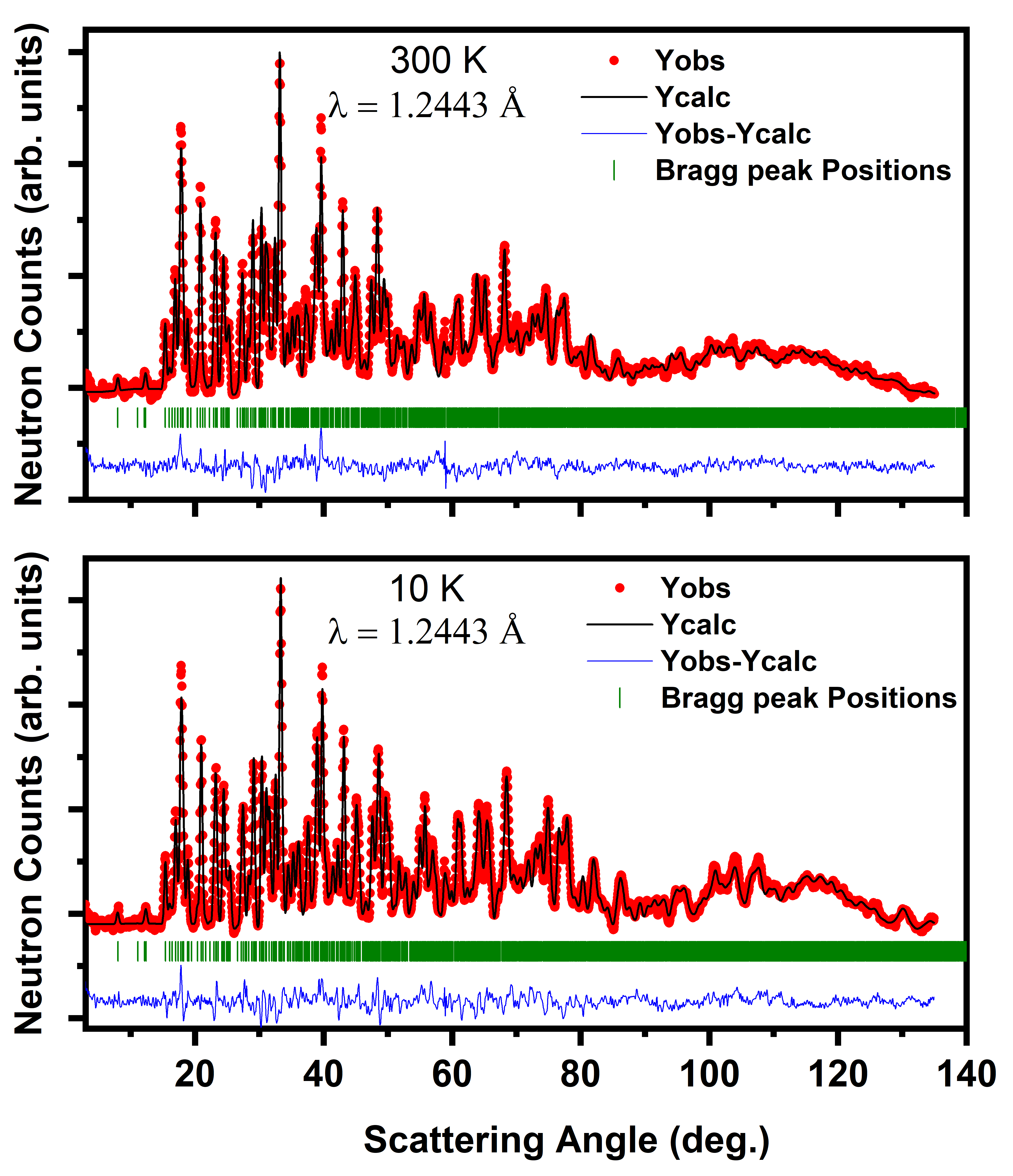
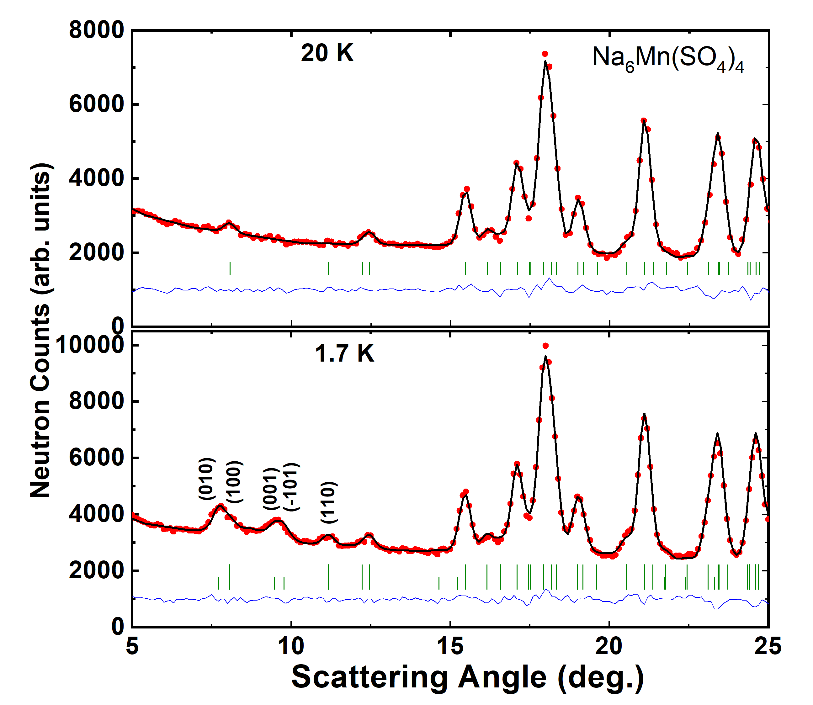
In order to further investigate the magnetic ground state of the material, neutron diffraction data were collected on bulk powder sample over the temperature range 1.7-300 K. Preparation of phase pure compound in sufficient quantity to perform neutron diffraction is rather challenging. However, almost 5 gm of single crystals were grown in different batches and these crystals were crushed to form polycrystalline powdered sample. Phase purity of bulk amount of powdered sample was checked via laboratory PXRD. The Rietveld refined neutron diffraction patterns measured at 300 K and 10 K are shown in Figure 5. The crystal structure for $Na_{6}Mn(SO_{4})_{4}$ remains monoclinic with space group $P2_{1}/c$ over the entire temperature range 1.7-300 K.

Figure 5: Rietveld refinement of Neutron diffraction patterns for $Na_{6}Mn(SO_{4})_{4}$ measured at (top) 300 K and (bottom) 10 K.

Figure 6: Low-temperature neutron diffraction patterns down to 1.7 K

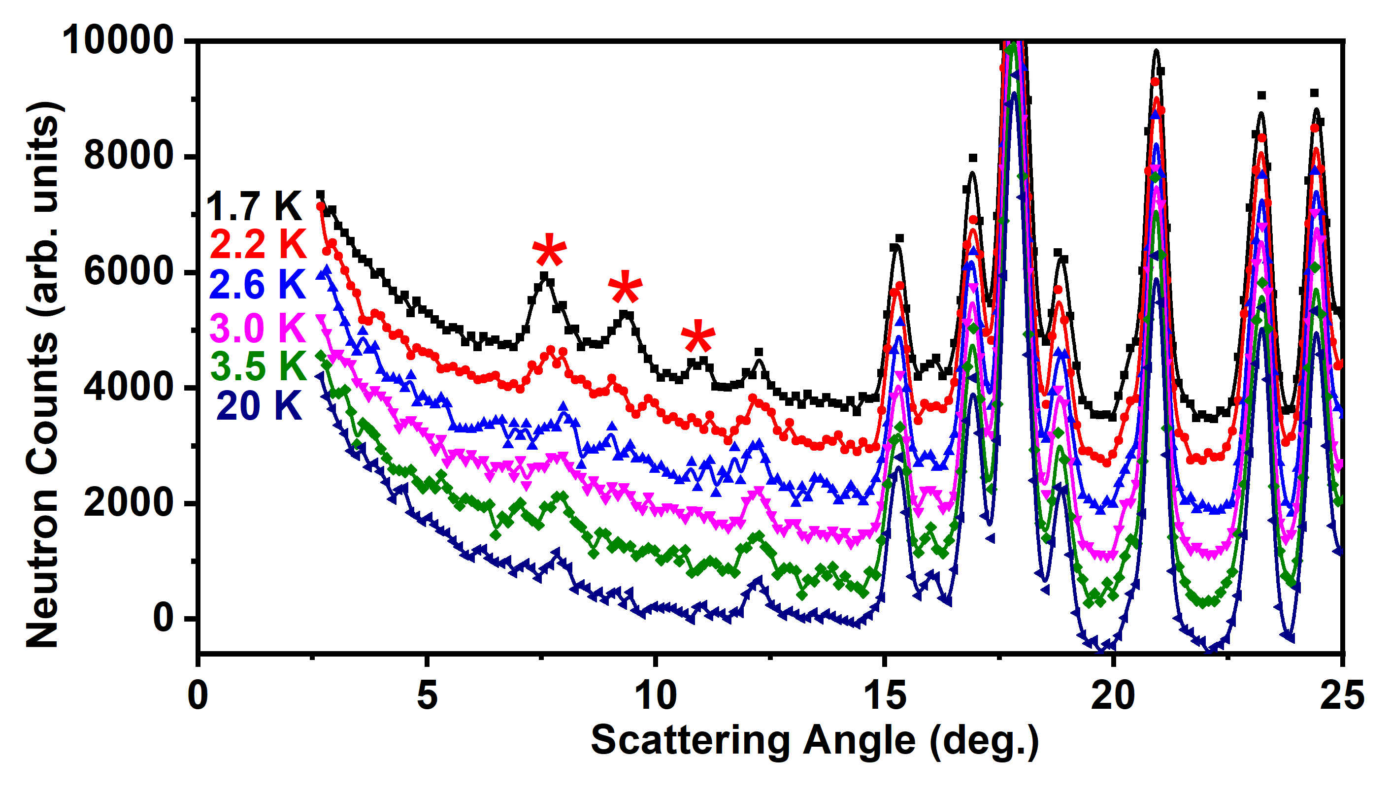
In order to probe the long-range antiferromagnetic interaction in $Na_{6}Mn(SO_{4})_{4}$, neutron diffraction data were collected down to 1.7 K (Figure 6). The appearance of additional magnetic Bragg peaks at $2\theta~{}\sim$ 7.6^∘, 9.4^∘, and 11^∘ (Marked with asterisks in Figure 6) below 3 K confirms a long-range antiferromagnetic ordering of the material.

All magnetic reflections observed for $Na_{6}Mn(SO_{4})_{4}$ could be indexed with a propagation vector k = (0,0,0) with respect to the same monoclinic unit cell as the nuclear structure. The symmetry-allowed magnetic structure is determined by a representation analysis, as applied for various kinds of spin systems Bera-PRB-2022 ; Suresh-PRB-2018 ; Bera-PRB-2017 ; Bera-PRB-2016 , using the program BASIREPS available with the FULLPROF program suite Carvajal-PB . The results of the symmetry analysis reveal that there are four irreducible representations (IRs). Among the four IRs, the IR(1) or $\Gamma_{1}$ and IR(3) or $\Gamma_{3}$ are non-zero for the magnetic site of the present compound. Therefore, there are two possible symmetry allowed magnetic structures for $Na_{6}Mn(SO_{4})_{4}$. Both the IRs $\Gamma_{1}$ and $\Gamma_{3}$ are one-dimensional.

Table 3: Basis vectors of the magnetic sites of Mn with the propagation vector k = (0 0 0) for $Na_{6}Mn(SO_{4})_{4}$. Only the real components of the basis vectors are presented. The two atoms of the non-primitive basis are defined according to Mn-1 (x, y, z):(0.5, 0, 0.5) and Mn-2 (-x, y+1/2, -z+1/2): (-0.5, 0.5, 0).

IRs		Basis vectors
		Site (2$b$)
		Mn-1	Mn-2
$\Gamma_{1}$	$\Psi_{1}$	100	-100
	$\Psi_{2}$	010	010
	$\Psi_{3}$	001	00-1
$\Gamma_{2}$	$\Psi_{1}$	100	100
	$\Psi_{2}$	010	0-10
	$\Psi_{3}$	001	001

Figure 7: Experimentally observed (circles) and calculated (solid lines through the data points) neutron diffraction patterns for $Na_{6}Mn(SO_{4})_{4}$ at (top) 20 K (paramagnetic state) and (bottom) 1.7 K (magnetically ordered state), respectively. The solid lines at the bottom of each panel represent the difference between observed and calculated patterns. The vertical bars indicate the positions of allowed nuclear and magnetic [the bottom panel] Bragg peaks.

Figure 8: The magnetic structure of $Na_{6}Mn(SO_{4})_{4}$.

Figure 9: The temperature-dependent lattice parameters and unit cell volume of $Na_{6}Mn(SO_{4})_{4}$ over the temperature range 1.7-300 K.

The magnetic representation $\Gamma_{mag}$ is composed as

$$\Gamma_{mag}=3\Gamma_{1}+3\Gamma_{3}$$ (1)

The basis vectors (the Fourier components of the magnetization) for these two IRs $\Gamma_{1}$ and $\Gamma_{3}$ for the magnetic site are given in Table 3. The basis vectors are calculated using the projection operator technique implemented in the BASIREPS program Carvajal-PB ; Carvajal-Fullprof . Out of the $\Gamma_{1}$ and $\Gamma_{3}$, the best refinement of the magnetic diffraction pattern is obtained for the IR $\Gamma_{1}$. The refinement with the $\Gamma_{1}$ is shown in Figure 7. A good agreement is observed between observed and calculated pattern.

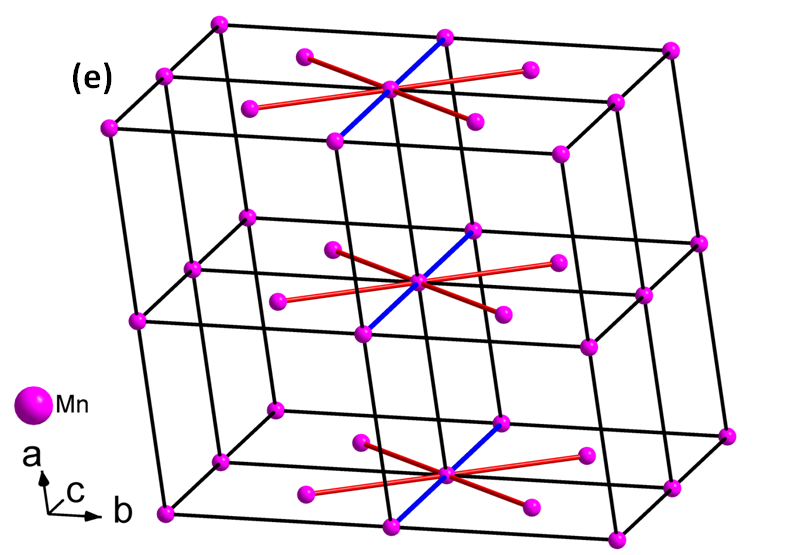
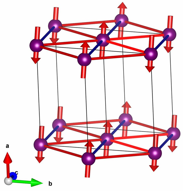
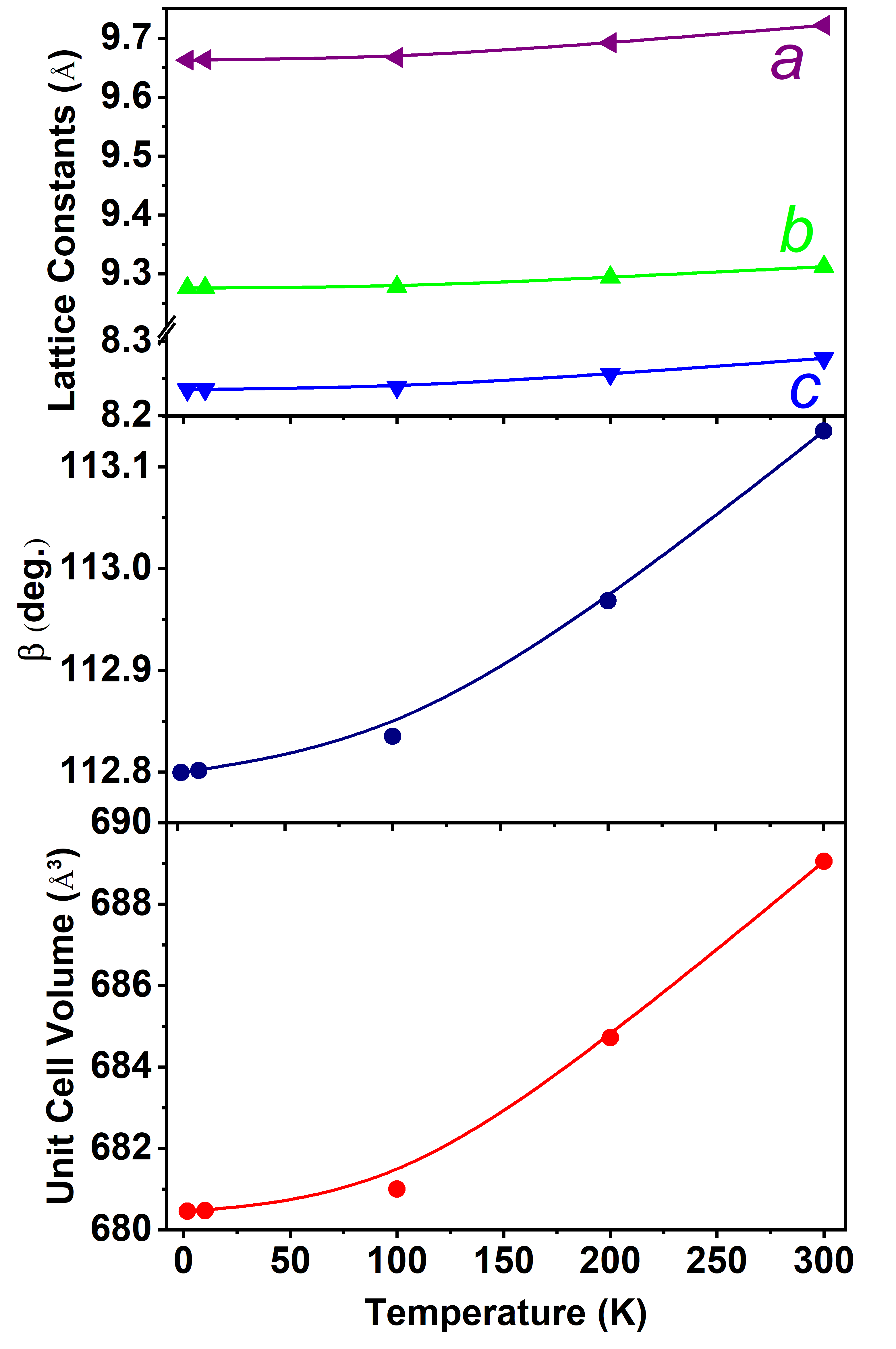
The corresponding magnetic structure is shown in Figure 8. The magnetic structure reveals antiferromagnetic chains of the Mn moments along the NN bond (red bonds) directions in the $bc$ plane, and such chains are coupled ferromagnetically along the NNN bond (blue bonds) directions in the $bc$ plane. Therefore, the magnetic structure within the $bc$ plane is a Néel type AFM. Such antiferromagnetic planes are stacked ferromagnetically along the $a$-axis (grey bonds). The magnetic structure is purely antiferromagnetic in nature without having any net magnetization per unit cell. The magnetic moments are lying in the $ac$ plane with moment components $m_{a}$ = 2.60(8) and $m_{c}$= 1.35(28) $\mu_{B}$ per magnetic site (Mn²⁺) along the $a$ and $c$ axes respectively. The net ordered site moment of Mn ions (considering all the components) is found to be $M_{total}$ = 2.42 (3) $\mu_{B}$/Mn²⁺ at 1.7 K. The magnetic moment is found to be strongly reduced from the theoretically expected value of 4 $\mu_{B}$/Mn²⁺ ($\sim$ 80 $\%$ of the fully ordered moment of 5 $\mu_{B}$/Mn²⁺) revealing the presence of a strong spin fluctuation at 1.7 K. The temperature variation of the lattice parameters and unit cell volume is shown in Figure 9. Change in slope at low temperature could be due to the interaction with magnetic spin and lattice.

III.3 Theoretical study of $Na_{6}Mn(SO_{4})_{4}$

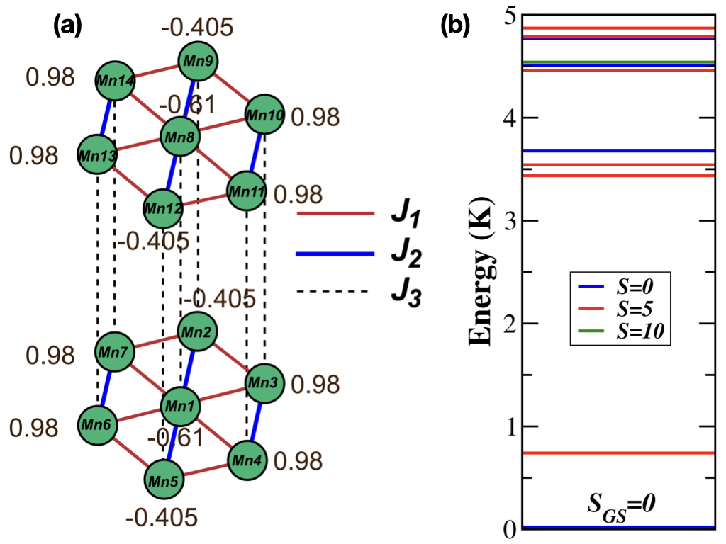
The refined X-ray diffraction data of $Na_{6}Mn(SO_{4})_{4}$ (Figure 1) shows a primitive monoclinic crystal structure in which $Mn^{2+}$ ions are placed at each corner of the unit cell and an additional $Mn^{2+}$ ion is located at the face-center position in the $bc$ plane. A careful analysis of the structural information reveals that any $Mn^{2+}$ ion located at the corner of the unit cell is connected to four first nearest neighbours along the face diagonal in $bc$ plane and two second neighbours along the $c$-axis. This arrangement repeats along the $a$-axis, as shown in the Figure 10a. Heisenberg Hamiltonian is solved on the minimum cluster which adequately represents the crystal. This involves fourteen $Mn^{2+}$ ions at the vertices and at the centre of two hexagons parallel to each other, as shown in Figure 10a. The spin of each $Mn^{2+}$ ion is 5/2 as the crystal field is weak. Exact diagonalization of the 14 site s = 5/2 spin Heisenberg system is computationally prohibitive as the number of spin orientations (dimensionality of the Fock space) is more than 78 billion. Hence we have replaced the s = 5/2 site spins by s = 1/2 site spins and have scaled the computed susceptibility by a factor of 11.67 which is the ratio of the square of the magnetic moments of a s = 5/2 ion and s = 1/2 ion. The Fock space dimension of the 14 spin-1/2 system is only 16,384. Furthermore, since z-component of the total spin, $S_{z}$ is conserved, we can factor the space into different $M_{S}$ sectors. Solving the eigen system for all the eigenvalues and eigenvectors is not compute intensive and affords exploring the parameter space of the exchange constants in the Hamiltonian on a fine grid.

Figure 10: (a) Schematic of the magnetic exchange interactions in $Na_{6}Mn(SO_{4})_{4}$. The spin densities of $S$=5, $M_{S}$=+5 state are also shown. The spin density at each Mn site is scaled by a factor of 5 to convert from $s$=1/2 to $s$=5/2 site spin, (b) Low-lying energy eigen states of our model in Kelvin along with the total spin of the state, and (c) Magnetic susceptibility ($\chi T$) as a function of temperature. Experimental points are shown by circles and calculated values fall on the red line. Blue line indicates the expected $\chi T$ value for free $s$=5/2 moments.

The magnetic properties are modelled by employing the Heisenberg spin Hamiltonian,

$$\hat{H}_{o} = -J_{1}(\hat{\vec{s}}_{1}\cdot\hat{\vec{s}}_{3}+\hat{\vec{s}}_{1}\cdot\hat{\vec{s}}_{4}+\hat{\vec{s}}_{1}\cdot\hat{\vec{s}}_{6}+\hat{\vec{s}}_{1}\cdot\hat{\vec{s}}_{7}+\hat{\vec{s}}_{2}\cdot\hat{\vec{s}}_{3}$$ (2)

$$+\hat{\vec{s}}_{4}\cdot\hat{\vec{s}}_{5}+\hat{\vec{s}}_{5}\cdot\hat{\vec{s}}_{6}+\hat{\vec{s}}_{2}\cdot\hat{\vec{s}}_{7}+\hat{\vec{s}}_{8}\cdot\hat{\vec{s}}_{10}+\hat{\vec{s}}_{8}\cdot\hat{\vec{s}}_{11}$$

$$+\hat{\vec{s}}_{8}\cdot\hat{\vec{s}}_{13}+\hat{\vec{s}}_{8}\cdot\hat{\vec{s}}_{14}+\hat{\vec{s}}_{9}\cdot\hat{\vec{s}}_{10}+\hat{\vec{s}}_{11}\cdot\hat{\vec{s}}_{12}+\hat{\vec{s}}_{12}\cdot\hat{\vec{s}}_{13}$$

$$+\hat{\vec{s}}_{9}\cdot\hat{\vec{s}}_{14})-J_{2}(\hat{\vec{s}}_{1}\cdot\hat{\vec{s}}_{2}+\hat{\vec{s}}_{3}\cdot\hat{\vec{s}}_{4}+\hat{\vec{s}}_{1}\cdot\hat{\vec{s}}_{5}+\hat{\vec{s}}_{6}\cdot\hat{\vec{s}}_{7}$$

$$+\hat{\vec{s}}_{8}\cdot\hat{\vec{s}}_{9}+\hat{\vec{s}}_{10}\cdot\hat{\vec{s}}_{11}+\hat{\vec{s}}_{8}\cdot\hat{\vec{s}}_{12}+\hat{\vec{s}}_{13}\cdot\hat{\vec{s}}_{14})-J_{3}(\hat{\vec{s}}_{1}\cdot\hat{\vec{s}}_{8}$$

$$+\hat{\vec{s}}_{2}\cdot\hat{\vec{s}}_{9}+\hat{\vec{s}}_{3}\cdot\hat{\vec{s}}_{10}+\hat{\vec{s}}_{4}\cdot\hat{\vec{s}}_{11}+\hat{\vec{s}}_{5}\cdot\hat{\vec{s}}_{12}+\hat{\vec{s}}_{6}\cdot\hat{\vec{s}}_{13}$$

$$+\hat{\vec{s}}_{7}\cdot\hat{\vec{s}}_{14})$$

where, $J_{1}$, $J_{2}$ and $J_{3}$ are the strength of exchange interactions between first, second and third neighbours, respectively and $\hat{\vec{s}}$ are the site spin operators and the numbers in the subscript represent the site index as in Figure 10a. A positive or negative value of $J$ corresponds to a ferromagnetic or antiferromagnetic exchange interaction respectively. The three unique exchange parameters $J_{1}$, $J_{2}$ and $J_{3}$ are all antiferromagnetic and have their strengths that are exponentially dependent on the distance between ions; hence $|J_{1}|>|J_{2}|>|J_{3}|$. The exchange constants $J_{2}$ and $J_{3}$ are expressed as fractions of $J_{1}$, which is set to -1.0. We have taken the two exchange constants $J_{2}$ and $J_{3}$ as $J_{2}=-e^{-\frac{r_{2}}{r_{1}}}$ and $J_{3}=-e^{-\frac{r_{3}}{r_{1}}}$, where $r_{1}$, $r_{2}$ and $r_{3}$ are the first, second and third neighbour distances from the refined X-ray diffraction data. As the first neighbour Mn-O-O-Mn dihedral angle is about 148^∘ (from X-ray structure), we take $J_{1}$ to be antiferromagnetic.

The matrix of the spin Hamiltonian (eq. 2) was constructed using a basis with constant total $M_{S}$. The largest Hamiltonian matrix which is 3432 x 3432 corresponds to the $M_{S}=0$ sector. We obtain the complete eigen spectrum in all the $M_{S}$ sectors; this is used to compute the magnetic susceptibility of the system. As the magnetic measurements are carried out under an applied magnetic field, we include a Zeeman term in our calculation which contributes an energy $-g\mu_{B}H_{z}M_{S}$ to the eigenstates in a given $M_{S}$ sector; $g$ is the gyromagnetic ratio, $\mu_{B}$ is the Bohr magneton and $H_{z}$ is the applied magnetic field. The magnetic susceptibility of the system is given by,

$$\chi T=\frac{N_{A}g^{2}\mu_{B}^{2}F(J,T)}{k_{B}}$$ (3)

$$F(J,T)=\langle M_{S}^{2}\rangle=\frac{\sum_{S}\sum_{M_{S}}M_{S}^{2}e^{-\frac{E_{o}(S,M_{S})}{k_{B}T}}}{\sum_{S}\sum_{M_{S}}e^{-\frac{E_{o}(S,M_{S})}{k_{B}T}}}$$ (4)

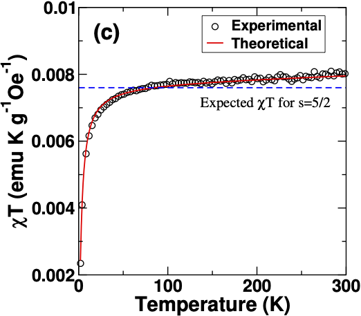
In the above expression $N_{A}$ is the Avogadro number, $k_{B}$ is the Boltzmann’s constant and $E_{o}(S,M_{S})$ are energies of the unperturbed Hamiltonian corresponding to the eigen state with z-component of total spin $M_{S}$ Kahn-Mol Mag . We also add a Curie contribution (C) to the total susceptibility to account for any unreacted residual spin moments left after the synthesis. Besides, our magnetic data shows that the high temperature susceptibility is larger than the 0.0076 emu K/(g Oe) expected for free spin-5/2 moments. The $\chi T$ value also shows a small linear increase with temperature, contrary to the temperature independent behaviour expected in the paramagnetic region for a Curie paramagnet. This suggests that there is an additional temperature independent susceptibility term or the van Vleck paramagnetic ($\chi_{VV}$) contribution coming from the excited states. The total $\chi T$ value is given by $\chi T=\chi T(ex)+\chi T(res)+\chi_{VV}T$.

The strength of various exchange interactions are obtained from the parameters that best fit the experimental magnetic data. The experimental magnetic data is fitted in the temperature range 2-300 K (Figure 10c) and best fit parameters correspond to $J_{1}$= -3.6 K, $J_{2}$ = -0.94 K, $J_{3}$ = -0.76 K, $g$ = 2.01, $C$ = 9 x 10^-5 emu K /(g Oe) and $\chi_{VV}$ = 8 x 10^-7 emu / (g Oe). The contribution to the susceptibilty from Curie like and temperature independent paramagnetic concentrations are less than the 3% of the paramagnetic susceptibility of the system obtained by turning off all the exchange interactions. The ground state of the system is a spin singlet ($S_{GS}$=0) (Figure 10b), confirming an overall antiferromagnetic interaction, as also evidenced from the decreasing $\chi T$ value as we approach zero Kelvin. The first excited state is an $S$=5 state (spin is scaled from s = 1/2 to s = 5/2) with an energy gap from the ground state of 0.74 K (Figure 10b). Besides, there are two more S = 5 states at 3.44 K and 3.54 K, before an excited singlet state is found at 3.68 K. Application of magnetic field can significantly lower the energies of states with non-zero magnetization belonging to this S = 5 multiplet. This can lead to trapping of moments in higher magnetization states when the system is cooled under the influence of magnetic field, resulting in the bifurcation of ZFC and FC curves. This is more dominant at low field strengths as the population of the high spin state is not saturated at these field strengths. Thus, for a small applied field, one observes a substantial change in magnetization on cooling. However, at high field strengths, at about 3 K, the high spin population is almost saturated and this will lead to smaller change in magnetization as the system is cooled. Hence the ZFC and FC susceptibility curves lie very close to each other. The first excited state with spin S = 5 at 0.74 K, has significant thermal population when cooled to 1.7 K which is the lowest temperature at which the study is carried out. The expectation values of the site $s_{z}$ operator in this S = 5 excited state spin manifold corresponding to $M_{S}$ = +5 for the best fit exchange parameter values are presented in the Figure 10a. Our computed spin densities are consistent with the magnetic structure obtained from the neutron diffraction measurement, which shows parallel spin arrangement along the $a$ and $c$ directions, while the moments are anti-parallel along the {011} direction.

IV CONCLUSIONS

In summary, the measurement of magnetic properties of a Vanthoffite mineral $Na_{6}Mn(SO_{4})_{4}$ shows antiferromagnetic characteristics below 3 K. Neutron diffraction refinements at 1.7 K clearly shows an antiferromagentic spin arrangement in $bc$-plane of the structure. Numerical results from full diagonalization approach support the experimental results and unambiguously show the presence of antiferromagntic interactions and singlet magnetic ground state in $Na_{6}Mn(SO_{4})_{4}$.

V ACKNOWLEDGEMENTS

T.N.G. and S.R. would like to thank DST and INSA for financial support. A.D. would like to thank IISc for funding.

References

- (1) A. K. Padhi, K. S. Nanjundaswamy, and J. B. Goodenough, J. Electrochem. Soc. 144, 1188 (1997).
- (2) J. Wang, and X. Sun, Energy Environ. Sci. 8, 1110 (2015).
- (3) C. Masquelier and L. Croguennec, Chem. Rev. 113, 6552 (2013).
- (4) B. C. Melot and J.-M. Tarascon, Acc. Chem. Res. 46, 1226 (2013).
- (5) Z. Gong and Y. Yang, Energy Environ. Sci. 4, 3223 (2011).
- (6) G. Rousse and J. M. Tarascon, Chem. Mater. 26, 394 (2014).
- (7) M. Reynaud, G. Rousse, J.-N. Chotard, J. Rodríguez-Carvajal, and J.-M. Tarascon, Inorg. Chem. 52, 10456 (2013).
- (8) M. Reynaud, J. Rodríguez-Carvajal, J.-N. Chotard, J.-M. Tarascon, and G. Rousse, Phys. Rev. B 89, 104419 (2014).
- (9) M. Sun, G. Rousse, A. M. Abakumov, M. Saubanere, M.-L. Doublet, J. Rodríguez-Carvajal, G. Van Tendeloo, and J.-M. Tarascon, Chem. Mater. 27, 3077 (2015).
- (10) G. Rousse, J. Rodríguez-Carvajal, C. Giacobbe, M. Sun, O. Vaccarelli, and G. Radtke, Phys. Rev. B 95, 144103 (2017).
- (11) L. Lander, M. Reynaud, J. Rodríguez-Carvajal, J.-M. Tarascon, and G. Rousse, Inorg. Chem. 55, 11760 (2016).
- (12) A. Furrer, A. Podlesnyak, J. M. Clemente-Juan, E. Pomjakushina, and H. U. Güdel, Phys. Rev. B 101, 224417 (2020).
- (13) R. Toft-Petersen, N. H. Andersen, H. Li, J. Li, W. Tian, S. L. Bud’ko, T. B. S. Jensen, C. Niedermayer, M. Laver, and O. Zaharko, Phys. Rev. B 85, 224415 (2012).
- (14) J. Li, W. Tian, Y. Chen, J. L. Zarestky, J. W. Lynn, and D. Vaknin, Phys. Rev. B 79, 144410 (2009).
- (15) T. H. O’Dell, Electron. Power 11, 266 (1965).
- (16) E. Fogh, R. Toft-Petersen, E. Ressouche, C. Niedermayer, S. L. Holm, M. Bartkowiak, O. Prokhnenko, S. Sloth, F. W. Isaksen, and D. Vaknin, Phys. Rev. B 96, 104420 (2017).
- (17) L. Lander, G. Rousse, A. M. Abakumov, M. Sougrati, G. Van Tendeloo, and J.-M. Tarascon, J. Mater. Chem. A 3, 19754 (2015).
- (18) A. Scaramucci, E. Bousquet, M. Fechner, M. Mostovoy, and N. A. Spaldin, Phys. Rev. Lett. 109, 197203 (2012).
- (19) I. Kornev, M. Bichurin, J.-P. Rivera, S. Gentil, H. Schmid, A. G. M. Jansen, and P. Wyder, Phys. Rev. B 62, 12247 (2000).
- (20) M. Fiebig, J. Phys. D. Appl. Phys. 38, R123 (2005).
- (21) B. B. Van Aken, J.-P. Rivera, H. Schmid, and M. Fiebig, Nature 449, 702 (2007).
- (22) E. Bousquet, N. A. Spaldin, and K. T. Delaney, Phys. Rev. Lett. 106, 107202 (2011).
- (23) J.-P. Rivera, Eur. Phys. J. B 71, 299 (2009).
- (24) G. Rousse, J. Rodríguez-Carvajal, C. Wurm, and C. Masquelier, Phys. Rev. B 88, 214433 (2013).
- (25) P. Yanda and A. Sundaresan, In Advances in the Chemistry and Physics of Materials: Overview of Selected Topics; World Scientific, 224, (2020)
- (26) G. T. Rado, J. M. Ferrari, and W. G. Maisch, Phys. Rev. B 29, 4041 (1984).
- (27) S. Bluck and H. G. Kahle, J. Phys. C Solid State Phys. 21, 5193 (1988).
- (28) D. Vaknin, J. L. Zarestky, L. L. Miller, J.-P. Rivera, and H. Schmid, Phys. Rev. B 65, 224414 (2002).
- (29) G. Rousse, J. Rodriguez-Carvajal, S. Patoux, and C. Masquelier, Chem. Mater. 15, 4082 (2003).
- (30) D. Vaknin, J. L. Zarestky, J.-P. Rivera, and H. Schmid, Phys. Rev. Lett. 92, 207201 (2004).
- (31) S. Gnewuch and E. E. Rodriguez, Inorg. Chem. 59, 5883 (2020).
- (32) E. Fogh, O. Zaharko, J. Schefer, C. Niedermayer, S. Holm-Dahlin, M. K. Sørensen, A. B. Kristensen, N. H. Andersen, D. Vaknin, N. B. Christensen, and R. Toft-Petersen, Phys. Rev. B 99, 104421 (2019).
- (33) P. W. Anderson, Phys. Rev. 115, 2 (1959).
- (34) J. Kanamori, J. Phys. Chem. Solids 10, 87 (1959).
- (35) J. B. Goodenough, Phys. Rev. 100, 564 (1955).
- (36) J. B. Goodenough, J. Phys. Chem. Solids 6, 287 (1958).
- (37) J. B. Goodenough, A. Wold, R. J. Arnott, and N. Menyuk, Phys. Rev. 124, 373 (1961).
- (38) G. Rousse, J. Rodriguez-Carvajal, C. Wurm, and C. Masquelier, Chem. Mater. 13, 4527 (2001).
- (39) B. C. Frazer and P. J. Brown, Phys. Rev. 125, 1283 (1962).
- (40) B. C. Melot, G. Rousse, J.-N. Chotard, M. Ati, J. Rodriguez-Carvajal, M. C. Kemei, and J.-M. Tarascon, Chem. Mater. 23, 2922 (2011).
- (41) B. C. Melot, J. N. Chotard, G. Rousse, M. Ati, M. Reynaud, and J. -M. Tarascon, Inorg. Chem. 50, 7662 (2011).
- (42) B. C. Melot, G. Rousse, J.-N. Chotard, M. C. Kemei, J. Rodriguez-Carvajal, and J.-M. Tarascon, Phys. Rev. B 85, 94415 (2012).
- (43) G. Rousse, J. Rodriguez-Carvajal, C. Wurm, and C. Masquelier, Solid state Sci. 4, 973 (2002).
- (44) G. Rousse, J. Rodriguez-Carvajal, C. Wurm, and C. Masquelier, Appl. Phys. A 74, s704 (2002).
- (45) L. Tao, J. R. Neilson, B. C. Melot, T. M. McQueen, C. Masquelier, and G. Rousse, Inorg. Chem. 52, 11966 (2013).
- (46) K. L. Keester and W. Eysel, Acta Crystallogr. Sect. B: Struct. Crystallogr. Cryst. Chem. 33, 306 (1977).
- (47) A. Dutta, D. Swain, J. Sunil, C. Narayana, and T. N. Guru Row, Inorg. Chem. 59, 8424 (2020).
- (48) V. Sharma, D. Swain, and T. N. Guru Row, Inorg. Chem. 56, 6048 (2017).
- (49) T. Degen, M. Sadki, E. Bron, U. Konig, and G. Nenert, Powder Diffr. 29, S13 (2014).
- (50) V. Petricek, M. Dusek, and L. Palatinus, Zeitschrift für Krist. Mater. 229, 345 (2014).
- (51) V. Siruguri, S. M. Yusuf, and V. C. Rakhecha, Neutron News 11, 4 (2000).
- (52) J. Rodriguez-Carvajal, Physica B 192, 55 (1993).
- (53) A. K. Bera and S. M. Yusuf, J. Phys. Chem. C 124, 4421 (2020).
- (54) A. K. Bera, S. M. Yusuf, S. S. Meena, C. Sow, P. S. A. Kumar, and S. Banerjee, Mater. Res. Express 2, 026102 (2015).
- (55) A. K. Bera, S. M. Yusuf, and S. Banerjee, Solid State Sci. 16, 57 (2013).
- (56) R. Saha, A. Shireen, A. K. Bera, S. N. Shirodkar, Y. Sundarayya, N. Kalarikkal, S. M. Yusuf, U. V. Waghmare, A. Sundaresan, and C. N. R. Rao, J. Solid State Chem. 184, 494 (2011).
- (57) M. Paul Brian, Am. Mineral. J. Earth Planet. Mater. 58, 32 (1973).
- (58) H. Lu, C. Xiao, R. Song, T. Li, A. E. Maughan, A. Levin, R. Brunecky, J. J. Berry, D. B. Mitzi, V. Blum, and M. C. Beard, J. Am. Chem. Soc., 142, 13030 (2020).
- (59) W. H. Baur, Acta Cryst. Sect. B: Struct. Crystallogr. Cryst. Chem. 30, 1195 (1974).
- (60) K. Robinson, G. V. Gibbs, and P. H. Ribbe, Science, 172, 567 (1971).
- (61) I. D. Brown and D. Altermatt, Acta Crystallogr. B 41, 244 (1985).
- (62) A. K. Bera, S. M. Yusuf, L. Keller, F. Yokaichiya, and J. R. Stewart, Phys. Rev. B 105, 014410 (2022).
- (63) P. Suresh, K. Vijaya Laxmi, A. K. Bera, S. M. Yusuf, B. L. Chittari, J. Jung, and P. S. Anil Kumar, Phys. Rev. B 97, 184419 (2018).
- (64) A. K. Bera, S. M. Yusuf, A. Kumar, and C. Ritter, Phys. Rev. B 95, 094424 (2017).
- (65) A. K. Bera, S. M. Yusuf, A. Kumar, M. Majumder, K. Ghoshray, and L. Keller, Phys. Rev. B 93, 184409 (2016).
- (66) J. Rodriguez-Carvajal, FULLPROF suite, www.ill.eu/sites/fullprof/.
- (67) O. Kahn, Molecular Magnetism. VCH Publ. Inc.(USA), 393 (1993).