Social adaptive behavior and oscillatory prevalence in an epidemic model on evolving random geometric graphs

Abstract

Our recent experience with the COVID-19 pandemic amply shows that spatial effects like the mobility of agents and average interpersonal distance, together with adaptation of agents, are very important in deciding the outcome of epidemic dynamics. Structural and dynamical aspects of random geometric graphs are widely employed in describing processes with a spatial dependence, such as the spread of an airborne disease. In this work, we investigate the interplay between spatial factors, such as agent mobility and average interpersonal distance, and the adaptive responses of individuals to an ongoing epidemic within the framework of random geometric graphs. We show that such spatial factors, together with the adaptive behavior of the agents in response to the prevailing level of global epidemic, can give rise to oscillatory prevalence even with the classical SIR framework. We characterize in detail the effects of social adaptation and mobility of agents on the disease dynamics and obtain the threshold values. We also study the effects of delayed adaptive response of agents on epidemic dynamics. We show that a delay in executing non-pharmaceutical spatial mitigation strategies can amplify oscillatory prevalence tendencies and can have non-linear effects on peak prevalence. This underscores the importance of early implementation of adaptive strategies coupled with the dissemination of real-time prevalence information to effectively manage and control the epidemic.

I Introduction

Epidemics have always been a threat to humanity since ancient times. The black death wiped out two-thirds of the European population in the $14^{th}$ century blackdeath . COVID-19 has so far caused more than 6.9 million deaths coronadata . Understanding and controlling such events is therefore of paramount importance for our own survival on Earth. The dynamics of epidemics have been analyzed using various types of mathematical and computational models. Such models are of immense importance as they can give us quantitative insights into the dynamic process of an epidemic. Together with the knowledge generated in various other disciplines and field data, models help us to make informed decisions to effectively deal with a pandemic. The information gained from models of epidemics which incorporate pharmaceutical and non-pharmaceutical interventions are important in order to have better control over the epidemic Gatto2020 ; Colizza2007 ; Ahmed2021 ; Lang2018 .

The major type of mathematical model of the epidemic is the compartmental model in which a population is divided into various compartments such as S (Susceptible), I (Infected), R (Recovered), etc, based on the state of infection of individuals. In the simplest setting, such models constitute a set of rate equations for the fraction of individuals in various compartments and are mean-field in nature Ottar2018 ; Keeling2008 ; Rothman2008 . Real-world population structures are different from the ones typically considered in the mean-field equations of compartmental models. In a more realistic setting, population structure is modeled as a network in which individuals are the nodes and connections are the links of a complex network. In the network, two individuals are assumed to be ‘connected’ if the disease can be transmitted between them. Models of epidemic spread on such topological networks have been extensively investigated in the past Cohen2010 ; Pastor2015 ; Turner2020 .

In many real-world settings, spatial factors such as the average distance between individuals and their mobility play a crucial part in deciding the structure of a contact network and will influence any dynamic process defined on such a network. The networks where the connectivity is decided by a distance-dependent measure are called random geometric graphs Barthelemy2011 ; Penrose2007 . Such spatial factors, which are normally not considered in epidemic models on topological networks, have gained increased recent attention in the wake of the COVID19 pandemic loring2020 ; wong2020 ; chang2021 ; pujari2020 ; Melin2020 ; Kang2020 . In such spatial network models of the epidemic, individuals or nodes are embedded in 2D space in which connections exist between two nodes only if they are closer than a characteristic distance or the transmission range of a disease. The value of the characteristic distance can vary from zero for a disease that transmits only by person-to-person direct contact up to several meters for airborne diseases. The characteristic distance may also depend upon certain preventive strategies adopted by individuals, such as mask usage. So the structure of the contact network, in general, will be dynamic as well as disease-dependent. Thus models of epidemics on spatial networks can give us valuable insights into the dynamics of a disease in a population by incorporating factors like the mobility of individuals and other adaptive intervention strategies.

Various pharmaceutical and non-pharmaceutical intervention strategies can be employed to control an epidemic. For an air-born disease like COVID-19, mask usage, social distancing, and mobility restrictions are some of the most important non-pharmaceutical techniques that can be used to control the epidemic. Such intervention actions will have a direct bearing on the contact structure of the population Vrugt2020 ; Maier2020 ; Nowak2011 ; Arthur2021 ; Havlin2020 ; Paulo2022 ; Lopez2020 ; Caley2008 ; Funk2009 . Mask usage will reduce the ‘connectivity’ of the network by reducing the transmission range of viral particles between persons. Social distancing and mobility restrictions will also reduce the connectivity or the mean degree of the network by keeping individuals apart, as in a low-density population. Since the effect of all such adaptive intervention actions are effectively the same, viz, reduction of connectivity of the network, we will refer to all such actions by the generic term ‘Social Adaptation’ (SA). Previous works which incorporate similar social adaptation have shown that oscillations in prevalence can arise due to individual payoff-based game-theoretic considerations by the agents Glaubitz2020 ; Khazaei2021 ; Jianping2021 ; Just2018 ; Liu2021 . In this work, we investigate how the adoption of such non-pharmaceutical adaptive intervention strategies by the agents who are spatially distributed and are mobile, affects the outcome of SIR dynamics. The connectivity structure of agents is modeled by random geometric graphs, which evolves by the adaptive actions of individuals as well as their mobility. The adaptive action of agents is incorporated via a threshold model for social adaptation i.e. their decision to follow SA depends upon the level of global prevalence with respect to a threshold prevalence. We show that such adaptive actions by the agents can give rise to oscillations in the prevalence of the disease even with simple SIR dynamics. We quantitatively characterize the effectiveness of non-pharmaceutical adaptive intervention strategies in controlling the epidemic. We obtain conditions under which effective reduction in the peak prevalence can be obtained from numerical solutions as well as simulations. We also study the effect of delays in executing such non-pharmaceutical threshold-based SA strategies on the epidemic. In this case, we show that such delays accentuate oscillations in the prevalence and have a non-linear effect on the peak prevalence. Our study shows how spatial factors like mobility and average interpersonal distance together with the adaptive actions of the population - either voluntary or enforced- can give rise to epidemic waves in time.

The paper is organized as follows. In Sec. II, we introduce the SIR model on evolving random geometric graphs and discuss its threshold behavior. We characterize the effect of the mobility of agents on the SIR dynamics. In Sec. III, we discuss the effect of non-pharmaceutical adaptive strategies by the agents on the dynamics of the epidemic and how that leads to oscillations in the prevalence. In Sec. IV, we consider the effects of delays in implementing the adaptive strategies, followed by a discussion of our results in Sec. V.

II SIR dynamics on evolving Random Geometric Graphs

We will follow the works of Buscarino2008 ; Peng2019 ; Glaubitz2020 in defining an epidemic model with spatially distributed agents. We consider a spatial network in which $N$ individuals (nodes) are distributed uniformly and randomly in a square patch of length $L$ with density $\rho=\frac{N}{L^{2}}$. Two nodes are assumed to be ‘connected’ and can potentially pass on the disease if they are closer than a characteristic transmission range $b$. At each time step, an agent moves from its current location and assumes a new random position within a circular patch of radius $m_{0}$ with the current location as the center. This will lead to a new spatial connectivity structure at each time step. We call $m_{0}$ as mobility parameter. SIR dynamics is implemented on this evolving RGG where Susceptible (S), Infected (I), and Recovered (R) are the compartments. When $m_{0}=0$, the nodes are static. When $m_{0}\sim L$, over time, all the individuals interact with all others. These are the extreme cases of mobility. In addition to this, if we assume that the change in the connectivity structure of the network and the epidemic process happens at the same rate, we can write down mean-field equations to model the process. Let $\beta$ be the probability with which infection is transmitted to a neighbor of an infected individual, and $\gamma$ be the probability that an infected individual recovers from infection at any time step. At any time step $t$, the number of Susceptible, Infected, and Recovered agents are denoted by $S(t)$, $I(t)$, $R(t)$ such that

$$S(t)+I(t)+R(t)=N$$ (1)

or

$$s(t)+i(t)+r(t)=1$$ (2)

Where $s(t)=S(t)/N$, $i(t)=I(t)/N$, $r(t)=R(t)/N$ are the normalized values of the number of Susceptible, Infected, and Recovered agents, respectively. Now the probability of a susceptible agent not being infected by any of its infectious neighbors in a given time step is $(1-\beta)^{n}$ where $n=\rho\pi b^{2}i(t)$ is the average number of infected neighbors inside a disk of radius $b$. Therefore, the equations for the evolution of the fraction of agents in different compartments take the form,

$$s(t+1)=s(t)-s(t)[1-(1-\beta)^{\pi b^{2}\rho i(t)}]$$ (3)

$$i(t+1)=i(t)-\gamma i(t)+s(t)[1-(1-\beta)^{\pi b^{2}\rho i(t)}]$$ (4)

$$r(t+1)=r(t)+\gamma i(t)$$ (5)

For small values of $\beta$, Eq. 4 becomes,

$$i(t+1)\approx i(t)-\gamma i(t)+[1-i(t)-r(t)]\beta{\pi b^{2}\rho i(t)}$$ (6)

Since the recovered compartment $r(t)$ will be very small at the beginning of an epidemic, letting $r(t)\to 0$, Eq. 6 becomes,

$$i(t+1)\approx i(t)-\gamma i(t)+[1-i(t)]\beta{\pi b^{2}\rho i(t)}$$ (7)

Therefore for the epidemic to grow, we must have,

$$1-\gamma+\beta{\pi b^{2}\rho}\geq 1$$ (8)

Thus for a given density, the critical characteristic transmission range for an outbreak to happen is given by

$$b_{epi}=\sqrt{\frac{\gamma}{\rho\pi\beta}}$$ (9)

For values of $b$ above $b_{epi}$, epidemic outbreak happens and below it, epidemic cannot happen Buscarino2008 ; Peng2019 . It is instructive to compare the above critical transmission range with the condition for the formation of a giant connected component in a continuum percolation problem of overlapping discs with radius $b$. In the latter, overlapping discs of radius $b$ are randomly distributed in a plane with density $\rho$. When the value of the radius $b$ is sufficiently high, a giant connected component forms in the system signaling a phase transition. Denoting the critical radius of discs at which the transition occurs by $b_{gc}$, we know that Mertens2012

$$b_{gc}\approx\sqrt{\frac{1.128}{\pi\rho}}$$ (10)

When the radius is below the above critical value, no large connected component exists in the system. It is clear that, in a population with no mobility, $b_{gc}$ will act as a lower threshold value of the characteristic transmission range below which no epidemic spread can occur. However, when there is mobility, the lower threshold is given by Eq. 9. Therefore, we have the relation

$$b_{epi}\approx b_{gc}\sqrt{\frac{\gamma}{1.128\beta}}$$ (11)

Fig.1 shows the variation of the critical characteristic range $b_{epi}$ with the density of the population. For a given value of $\beta$ and $\gamma$, such a curve demarcates epidemic and non-epidemic regions.

Relaxing the assumptions about either the mobility or the rate of the two processes will require explicit consideration of the network structure. We use Monte Carlo simulations in these cases to obtain the results. Especially we will consider the two extremes of mobility i.e. the cases of static agents ($m_{0}=0$) and fully mobile agents $m_{0}\sim L$.

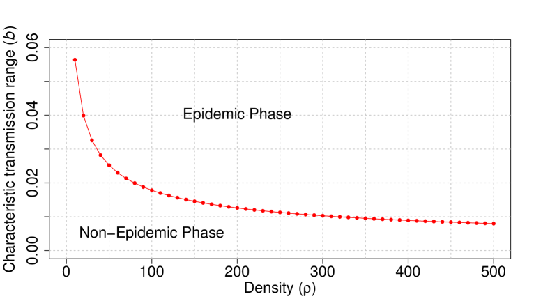
Figure 1: Variation of critical characteristic transmission range with density. The critical characteristic range is calculated using Eq. 9 for different values of density. Throughout the present work, we will use the values transmission probability $(\beta)$ = 0.5, recovery rate ($\gamma$) = 0.05, and density of agents $\rho=500$. An epidemic outbreak cannot happen in the region below the curve, whereas it is allowed above it.

Fig. 2 shows the prevalence over time curves for the cases with and without mobility of agents. In the present work, we will use the values, transmission probability $\beta=0.5$ and recovery rate $\gamma=0.05$. This means that there is a $50\%$ chance that a susceptible person who is within the characteristic range of an infected person will get the disease, and the average number of days for recovery is 20. Changing these values does not affect the qualitative nature of the results. From the figure, we can see that the mobility of agents has a pronounced effect on both the peak prevalence and the duration of the epidemic. We can see that the peak prevalence more than doubled when the agents are fully mobile.

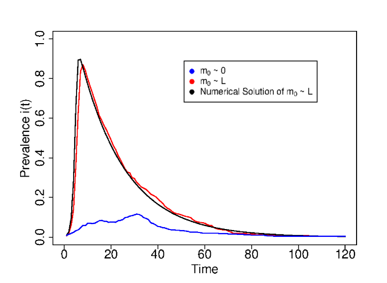
Figure 2: Variation of prevalence with time. Prevalence $i(t)$ is plotted for numerical and simulated solutions of an epidemic with mobility $m_{0}\sim L$. Simulation result is also shown for the case where the agents are not mobile $m_{0}=0$. Characteristic transmission range $b=0.05$.

Note that for a given disease, both $\beta$ and $\gamma$ are fixed quantities over which we do not have any control in general. Two controllable parameters here are the characteristic range $b$ and the density of agents $\rho$ (Another potentially controllable parameter is $m_{0}$). Characteristic range $b$ may be altered by measures such as mask usage while $\rho$ may be altered by measures such as social distancing or lock-downs. Note that a change in $b$ can also be viewed as a corresponding change in the density $\rho$. Fig. 3 shows the variation of peak prevalence with the characteristic range. Again, we compare the results with the case in which there is no mobility ($m_{0}=0$). The cases $m_{0}=0$ and $m_{0}\sim L$ act as two extreme scenarios, and we anticipate an intermediate behavior in the case of a population with in-between values for the mobility parameter $m_{0}$.

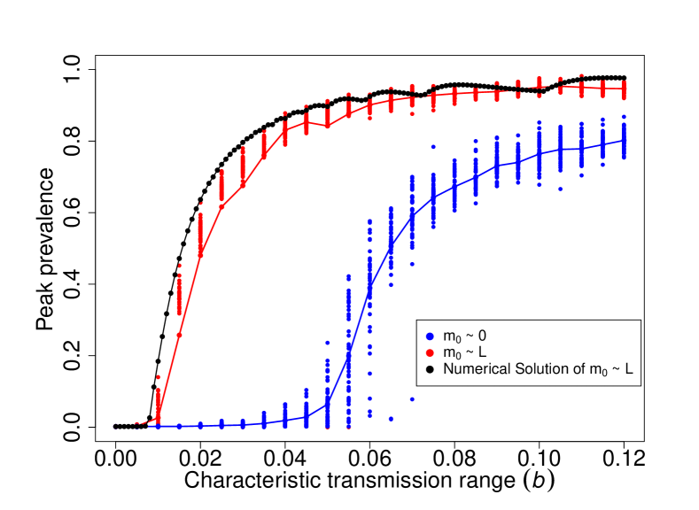
Figure 3: Variation of peak prevalence with characteristic transmission range. Variation of peak prevalence with characteristic transmission range $b$ is shown for $m_{0}=0$ and $m_{0}\sim L$. Simulation results are compared with the numerical solution for the case $m_{0}\sim L$.

III Effect of threshold-based adaptation strategies on the epidemic

An effective non-pharmaceutical intervention strategy to contain a disease like COVID-19, which can transmit from person to person via air, is to reduce the average effective interpersonal distance in a population. Measures such as mask usage, promoting social distancing, or partial or complete lock-downs are all examples of such adaptive strategies. Such measures could be either self-imposed by the agents or imposed by an external agency. Such measures are usually imposed and removed depending on the prevalence of the disease in the population although this may not be the sole criteria based on which such decisions are made. Ideally, we would like such strategies to have the effect that the average Euclidean distance between the individuals in the population becomes greater than the characteristic transmission range of the disease. For a given disease, we may view non-pharmaceutical intervention strategies as either (a) Increase the average distance between the agents or (b) Reduce the transmission range of the disease $b$. The first method can be implemented by assuming that the length of the system is increased by a factor of $f$ while keeping the number of agents the same when the agents follow social adaptation such that the mean distance between individuals increases by a factor of $f$ where $f\geq 1$. So the density changes from $\rho=\frac{N}{L^{2}}$ to $\rho^{SA}=\frac{N}{(Lf)^{2}}$ where $\rho^{SA}$ is the density of the agents while following social-adaptation strategies. The second method can be implemented by assuming that the characteristic transmission range $b$ is reduced by a factor of $1/f$. While both methods are mathematically the same, the latter describes situations like using face masks which effectively reduce the transmission range of the disease. Here, we will employ a reduction of $b$ to implement SA and will call $f$ as the SA factor.

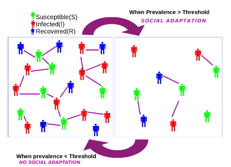
Figure 4: Schematic representation of the adaptive behavior of agents in the model. Agents are distributed spatially in a 2D square patch of size $L\times L$ with a density $\rho$ and move around. Agents employ social adaptation whenever the global prevalence of the disease is greater than a threshold $i_{c}$ and discard it otherwise. Adaptation results in larger interpersonal distance between the agents which is equivalent to a reduction in the density of the agents (see text).

We assume that agents or a central agency monitor the level of global prevalence in the population. Whenever the epidemic prevalence goes above a pre-defined threshold value $i_{c}$, agents follow social distancing from the next time step till the prevalence is reduced below the threshold (See Fig. 4). The characteristic transmission range $b$ then evolves according to,

$$b(t+1)=\left\{\begin{array}[]{@{}ll@{}}\ \frac{b(t)}{f},&{if}\ i(t)>i_{c}\\ b(t),&{otherwise}\end{array}\right.$$ (12)

where $b(0)$ is the original characteristic transmission range of the disease in the absence of any SA. The mean degree of the network thus assumes either of the two values $\rho\pi b^{2}$ and $\frac{1}{f^{2}}\rho\pi b^{2}$ depending upon the prevalence at any time step.

We will first consider the situation of $m_{0}\sim L$. In this case, Fig. 5 gives a comparison of the prevalence with and without SA. As we increase the SA factor $f$, the peak prevalence continues to drop, but a significant drop in the peak prevalence is achieved only beyond a critical value of $f$ ($f\approx 6$ in the figure). This can be understood based on the fact that for lower values of $f$, there is still an effective giant cluster in the system aiding the epidemic to spread. In other words, SA is not enough to bring the system below the critical line in Fig. 1. As the value of $f$ goes beyond the critical value, we can see that the prevalence oscillates around the threshold value $i_{c}$, which indicates that the characteristic transmission range went below its critical value. The threshold value of $f$, say $f_{th}$ is related to the critical value of the characteristic transmission range $b_{epi}$ by

$$f_{th}=b_{epi}\sqrt{\frac{\rho\pi\beta}{\gamma}}$$ (13)

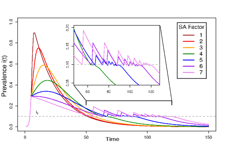
Figure 5: Numerical solution of prevalence as a function of time for various values of social adaptation factor $f$ with mobility $m_{0}\sim L$. $f=1$ corresponds to the case with no adaptive measures employed. $b(0)=0.05$.

Fig. 6 shows the variation of peak prevalence with the SA factor $f$. As we increase the value of $f$, peak prevalence reduces till the critical value of $f$, and thereafter the peak prevalence stagnates. A further increase of $f$ is not effective in reducing the peak prevalence and is not optimal from a socio-economic point of view as it imposes additional restrictions on the population without any additional benefits.

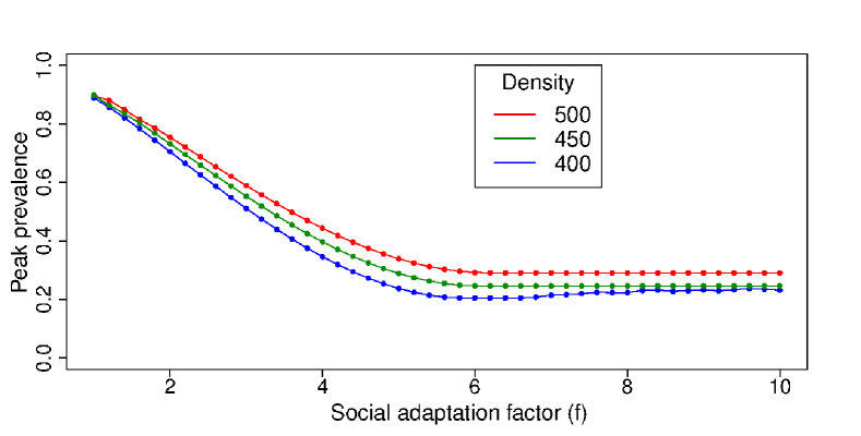
Figure 6: Numerical solution for variation of peak prevalence with social adaptation factor $f$ for various values of densities $\rho$. $m_{0}\sim L$, $b(0)=0.05$ and threshold $i_{c}=0.1$.

It is instructive to look at the peak prevalence as a function of the initial characteristic transmission range $b(0)$ for different values of the social distancing factor $f$, which is shown in Fig. 7. We can see that the peak prevalence becomes non-zero above the critical threshold given by Eq. 9. However, for a particular value of $f$, the peak prevalence is contained at the threshold value $i_{c}$ for a range of values of $b(0)$. As we further increase $b(0)$, the adaptation is no longer effective in controlling the epidemic, and the peak prevalence again rises after a specific value of $b(0)$. For higher values of $f$, the range over which the peak prevalence remains at the threshold value is also higher. The behavior can be understood based on the critical characteristic range $b_{epi}$ given in Eq. 9. The peak prevalence is contained at the threshold $i_{c}$ only when the adaptation brings the effective interpersonal distance to values below $b_{epi}$.

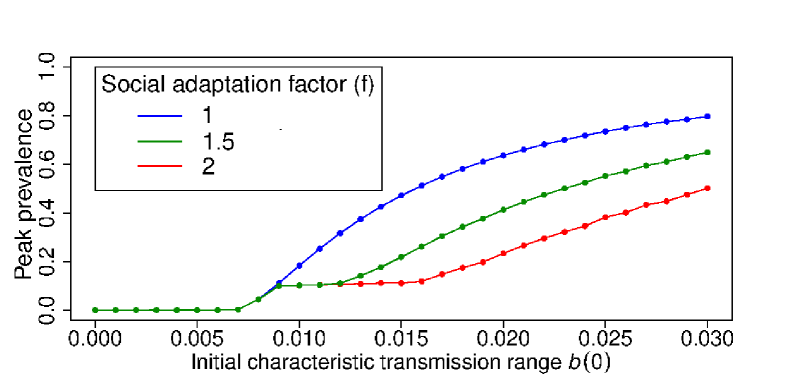
Figure 7: Numerical solution for variation of peak prevalence with initial characteristic transmission range $b(0)$ for various values of social adaptation factor $f$. $m_{0}\sim L$ and $i_{c}=0.1$.

We further extend the model to include a lower threshold for the removal of the social adaptation as well. Fig. 8 gives a comparison of the prevalence with and without SA with an upper threshold and a lower threshold. As we increase the SA factor $f$, the peak prevalence continues to drop, but a significant drop in the peak prevalence is achieved only beyond a critical value of $f$ ($f\approx 4$ in the figure). Here, whenever the adaptation factor is large enough to reduce the characteristic transmission range to values below its critical value, oscillations in prevalence are seen with bigger amplitudes lying between the threshold values.

When the agents are static, i.e. when $m_{0}=0$, Fig. 9 gives the variation of peak prevalence with the initial characteristic transmission range $b(0)$ $i_{c}=0.1$. As we increase the SA factor from $1$ to $3$, the peak prevalence reduces but the plateau behavior seen for $m\sim L$ in Fig. 7 is less pronounced here. Fig. 10 shows the prevalence plots for various values of the SA factor. Oscillations in the prevalence are seen for higher values of the SA factor.

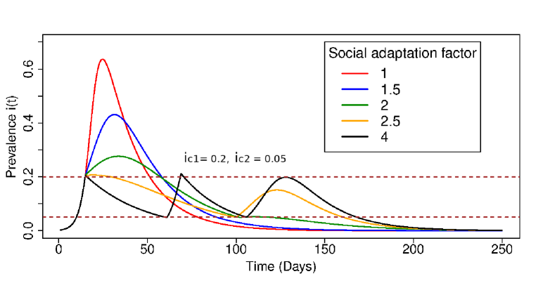
Figure 8: Numerical solution of prevalence as a function of time for various values of social adaptation factor $f$. $b(0)=0.02$ and $m_{0}\sim L$. $i_{c1}=0.2$ is the upper threshold and $i_{c2}=0.05$ is the lower threshold.

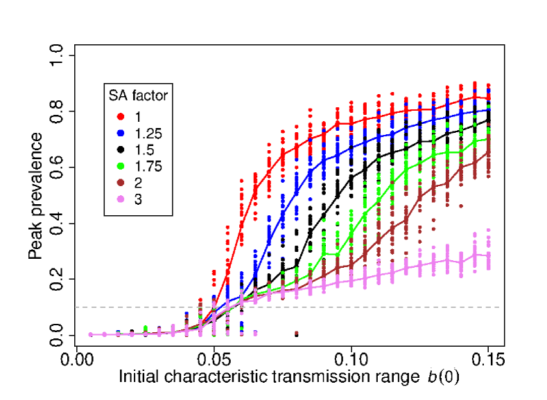
Figure 9: Simulation results of peak prevalence as a function of initial characteristic transmission range for different values of the social adaptation factor $f$. $i_{c}=0.1$ and $m_{0}=0$.

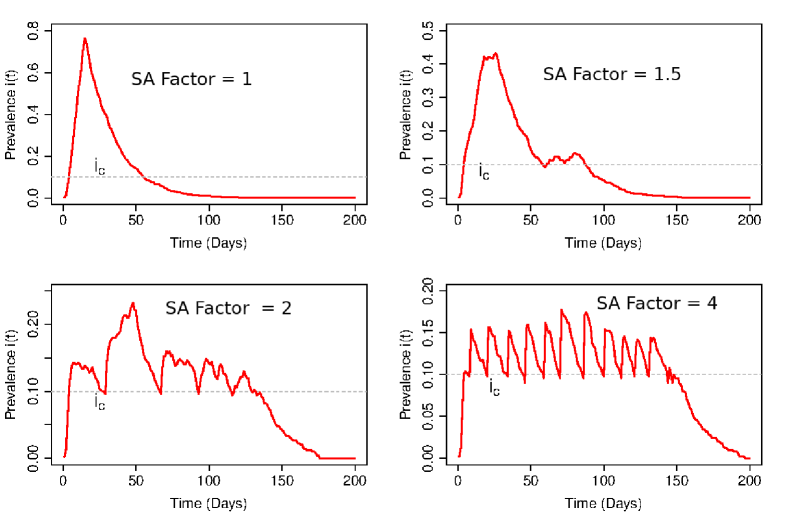
Figure 10: Typical simulation results for variation of prevalence with time for different values of the social adaptation factor. $i_{c}=0.1$, $m_{0}=0$, and $b(0)=0.1$.

IV Effect of delay in adaptation

So far we have assumed that the adaptive action by the agents is implemented without any delay. So whenever the prevalence crosses the threshold, the agents adapt in the very next time step. However, in practice, it is more likely that such adaptive action happens with a hold-up due to a delay in the transmission of information about the global prevalence or implementation delays. To account for such effects, we introduce a delay parameter so that if the prevalence goes above or below the threshold in a particular time step, the adaptive action by the agents happens only after a delay of $d$ time steps. We can imagine that such a delay can play a significant role in deciding the outcome of any attempt to control an epidemic. For highly contagious diseases, this delay can lead to situations where the infection has already affected a significant fraction of the population even before information about global prevalence is available, or any preventive action is taken. For a delay of $d$ time steps, we have

$$b(t+1+d)=\left\{\begin{array}[]{@{}ll@{}}\ \frac{b(t)}{f},&{if}\ i(t)>i_{c}\\ b(t),&{otherwise}\end{array}\right.$$ (14)

In Fig. 11 we show the numerical and simulation results of prevalence for various values of the delay parameter $d$. We can see that as the delay increases, peak prevalence rises significantly, and after a critical value of delay, adaptation becomes irrelevant. We can also see that bigger oscillations in the prevalence occur due to the combined effect of social adaptation and the delay. Variation of peak prevalence with $d$ for different $b(0)$ is shown in Fig. 12. We can clearly see the non-linear effect of the delay on peak prevalence, especially for larger values of $b(0)$. This shows the importance of implementing preventive measures with minimum delay, especially for diseases with higher values of transmission range.

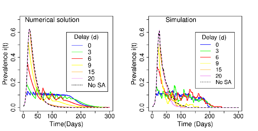
Figure 11: Variation of prevalence with time when there is a delay of $d$ time steps in implementing and removing SA. Results from numerical solution and simulation are shown. $m_{0}\sim L$, $i_{c}=0.1$, $b(0)=0.05$, $\beta=0.1$, and $\gamma=0.05$

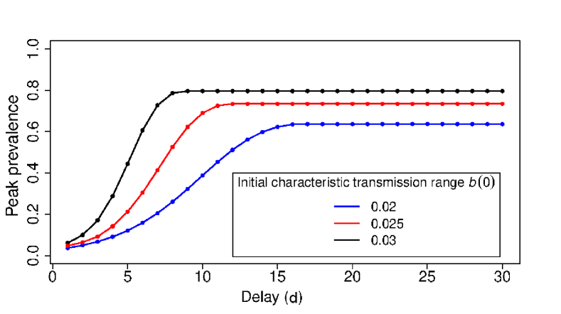
Figure 12: Variation of peak prevalence with the delay parameter $d$ for different values of the initial characteristic transmission range $b(0)$. $i_{c}=0.1$ and $f=4$.

V Discussion and Conclusion

Spatial effects like mobility and average interpersonal distance are very important in deciding the outcome of an epidemic dynamics, as amply shown by our recent experience with COVID-19. A number of recent works have discussed the effects of including the spatial aspects in the dynamic of an epidemic with adaptive agents Glaubitz2020 ; Liu2021 ; Khazaei2021 ; Just2018 . In general, we can use the framework of Random Geometric Graphs for modeling the spread of an epidemic incorporating spatial factors. The mobility of agents and their adaptation make the graphs evolving in time. In this work, we extended such models and considered agents who sense the global prevalence of the epidemic and take adaptive measures. Agents follow and discard social adaptation based on predefined prevalence thresholds. Our results show that such adaptation can have a significant effect on the trajectory of the epidemic dynamics. We characterize how different levels of adaptation by the agents affect the prevalence of the disease and the peak level of infection. Oscillatory prevalence is seen for a range of values of the adaptation parameter $f$. Our results also show that a delay in implementing the adaptation can have non-linear effects on peak prevalence which shows quantitatively that monitoring the global prevalence levels accurately is very crucial so that early intervention based on such information is possible. In particular, delay in disseminating information and/or delay in taking adaptive measures can accentuate oscillatory prevalence. Our results show how simple adaptation behavior by the agents can lead to waves during an epidemic even with SIR dynamics blue both in the case of fully mixed networks as well as static networks.

When spatial factors are included, the condition for an epidemic outbreak can be written as $1-\gamma+\beta\pi b^{2}\rho>1$ where $\rho$ is the density of the population and $b$ is the characteristic transmission range of disease. This helps to differentiate between factors that can be easily attributed to the disease itself (like $\gamma$, $\beta$) and factors related to how the agents are distributed over space (like the density $\rho$ or the average distance between the agents in the population). Since we can control the latter via various non-pharmaceutical strategies like social distancing, mask-wearing, partial or complete lockdown etc, the condition thus helps us to clearly define the target criteria in order to contain the propagation of disease.

In this work, we considered extreme scenarios where the agents are fully mobile or not mobile. We can easily extend the setting to consider situations where the mixing of agents is more gradual and/or limited spatially. A more realistic setting may be the one in which several patches of individuals are connected together by a few long-range connections with full mixing within each patch cornes2022 . We may also introduce heterogeneity in the population by considering distributions for parameters characterizing social adaptation, prevalence threshold, and mobility ellison2020 . This is especially relevant for mobility as infected individuals will, in general, be less mobile. Another obvious direction for future work is to consider the role of spatial adaptation in other models of epidemics like SEIR. Finally, it will be interesting to look at the effect of social adaption based on local information about the epidemic rather than the global one as considered in the present work. Going further, strategizing agents may be considered who will try to optimize individual adaptive actions based on information about the prevalence and the action of other agents Sharma2019 . We will explore some of these avenues in future work.

- (1) Austin Alchon, Suzanne. A pest in the land: new world epidemics in a global perspective. University of New Mexico Press: 21: 2003: ISBN 0-8263-2871-7.
- (2) Coronavirus database. Accessed 1 Aug 2022: https://www.worldometers.info/coronavirus/
- (3) Ahmed, Danish A. et al. Mechanistic modelling of COVID-19 and the impact of lockdowns on a short-time scale. PLOS ONE: 10: 16: 1-20: 2021.
- (4) Gatto, M. et al. Spread and dynamics of the Covid-19 epidemic in Italy: Effects of emergency containment measures. Proc. Natl. Acad. Sci. USA: 117: 10484-10491: 2020.
- (5) Colizza, V., Barrat, A., Barthelemy, M., Valleron, A.-J. & Vespignani, A. Modeling the worldwide spread of pandemic influenza: Baseline case and containment interventions. PLoS Med: 117: 4: e17: 2007.
- (6) Lang, John C et al. Analytic models for SIR disease spread on random spatial networks. Journal of Complex Networks: 6: 6: 948–970: 2018.
- (7) Ottar N Bjornstad. Epidemics, Models and Data using R. Springer International Publishing.: 2018.
- (8) Keeling MJ, Rohani P. Modeling infectious diseases in humans and animals. Princeton University Press: 2008.
- (9) Rothman, Kenneth J et al. Modern epidemiology. Wolters Kluwer Health/Lippincott Williams & Wilkins Philadelphia: 3: 2008.
- (10) Pastor-Satorras, R, Castellano, C., Van Mieghem, & P. Vespignani. Epidemic processes in complex networks. Rev. Mod. Phys: 87: 925: 2015.
- (11) Cohen, Reuven and Havlin, Shlomo. Complex networks: structure, robustness and function. Cambridge university press: 2010.
- (12) Turner, S., Klimek, P. Hanel, R.. A network-based explanation of why most covid-19 infection curves are linear. Proc. Natl. Acad. Sci. USA: 117:22684-22689: 2020.
- (13) Barthélemy, Marc. Spatial networks. Physics Reports: 499(1 –3): 1– 101: 2011.
- (14) Mathew Penrose. Random Geometric Graphs. Oxford Scholarship Online: ISBN-13: 9780198506263.
- (15) Thomas, Loring J et al. Spatial heterogeneity can lead to substantial local variations in COVID-19 timing and severity. Proc. Natl. Acad. Sci. U.S.A: 117: 24180–24187: 2020
- (16) Wong, David WS et al. Spreading of COVID-19: Density matters. Plos one: 15: 12: e0242398; 2020
- (17) Chang, Serina et al. Mobility network models of COVID-19 explain inequities and inform reopening. Nature: 589: 7840: 82–87: 2021
- (18) Pujari, Bhalchandra S and Shekatkar, Snehal M. Multi-city modeling of epidemics using spatial networks: Application to 2019-nCov (COVID-19) coronavirus in India. Medrxiv: 2020
- (19) Melin, Patricia et al. Analysis of spatial spread relationships of coronavirus (COVID-19) pandemic in the world using self organizing maps. Chaos, Solitons & Fractals: 138: 109914: 2020.
- (20) Kang, Dayun et al. Spatial epidemic dynamics of the COVID-19 outbreak in China. International Journal of Infectious Diseases: 94: 96 – 102: 2020.
- (21) te Vrugt, M., Bickmann, J. Wittkowski, R. Effects of social distancing and isolation on epidemic spreading modeled via dynamical density functional theory. Nat. Commun: 11: 5576: 2020.
- (22) Maier, B. F. & Brockmann, D. Effective containment explains sub exponential growth in recent confirmed covid-19 cases in china. Science: 368: 742-746: 2020.
- (23) Nowak B, Brzoska P et al. Adaptive Human Behavior in Epidemiological Models. Proc. Natl. Acad. Sci. USA: 03: 108: 6306-6311: 2011.
- (24) Arthur RF, Jones JH, Bonds MH, Ram Y, Feldman MW. Adaptive social contact rates induce complex dynamics during epidemics. PLOS Computational Biology: 17: 2: e1008639: 2021.
- (25) Havlin, Shlomo. Epidemic spreading and control strategies in spatial modular network. Applied Network Science: 95: 5: 1: 2020.
- (26) Paulo Cesar Ventura et al. Epidemic spreading in populations of mobile agents with adaptive behavioral response. Chaos, Solitons and Fractals: 156: 111849: 2022.
- (27) Lopez, Leonardo et al. The end of social confinement and COVID-19 re-emergence risk. Nature Human Behaviour: 4: 7: 746-755: 2020.
- (28) Funk, Sebastian et al. The spread of awareness and its impact on epidemic outbreaks. Proc. Natl. Acad. Sci. USA: 106: 16: 6872 - 6877: 2009.
- (29) Caley P, Philp DJ, McCracken K. Quantifying social distancing arising from pandemic influenza. Journal of the Royal Society Interface: 5: 23: 631-9: 2008.
- (30) Glaubitz Alina and Fu Feng. Oscillatory dynamics in the dilemma of social distancing. Proc. R. Soc. A: 67- 78: 2020.
- (31) H. Khazaei, K. Paarporn, A. Garcia and C. Eksin. Disease spread coupled with evolutionary social distancing dynamics can lead to growing oscillations. 2021 60th IEEE Conference on Decision and Control (CDC): 4280-4286: 2021.
- (32) Jianping Huang, Xiaoyue Liu et al. The oscillation-outbreaks characteristic of the COVID-19 pandemic . National Science Review: 8: 2021.
- (33) Just W, Saldana J, Xin Y. Oscillations in epidemic models with spread of awareness. J Math Biol: 76: 4: 1027-1057: 2018.
- (34) Liu Haoyan, Wang Xin, Liu Longzhao, Li Zhoujun. Co-evolutionary Game Dynamics of Competitive Cognitions and Public Opinion Environment . Frontiers in Physics: 9: 2021.
- (35) S. Triambak and D.P. Mahapatra. A random walk Monte Carlo simulation study of COVID-19-like infection spread. Physica A: Statistical Mechanics and its Applications: 9: 2021.
- (36) Goel, R., Bonnetain, L., Sharma, R. et al. Mobility-based SIR model for complex networks: with case study Of COVID-19. Soc. Netw. Anal. Min:11: 105:2021.
- (37) A. Buscarino et al. Disease spreading in populations of moving agents. Europhysics Letters: 82: 3: 38002: 2008.
- (38) Peng, Xiao-Long et al. An SIS epidemic model with vaccination in a dynamical contact network of mobile individuals with heterogeneous spatial constraints. Commun. Nonlinear Sci. Numer. Simulat: 73: 52 – 73: 2019.
- (39) Mertens, Stephan and Moore, Cristopher et al. Percolation threshold of a two-dimensional continuum system. Phys. Rev. E: 86: 6: 061109: 2012.
- (40) F.E. Cornes and G.A. Frank and C.O. Dorso. COVID-19 spreading under containment actions. Physica A: 588: 126566: 2022
- (41) G. Ellison. Implications of heterogeneous SIR models for analyses of COVID-19. tech. rep., National Bureau of Economic Research, 2020.
- (42) Sharma, Anupama et al. Epidemic prevalence information on social networks can mediate emergent collective outcomes in voluntary vaccine schemes. PLOS Computational Biology: 15: 5: 2019.