Learning Fair Models without Sensitive Attributes: A Generative Approach

Abstract

Most existing fair classifiers rely on sensitive attributes to achieve fairness. However, for many scenarios, we cannot obtain sensitive attributes due to privacy and legal issues. The lack of sensitive attributes challenges many existing works. Though we lack sensitive attributes, for many applications, there usually exists features/information of various formats that are relevant to sensitive attributes. For example, a person’s purchase history can reflect his/her race, which would be helpful for learning fair classifiers on race. However, the work on exploring relevant features for learning fair models without sensitive attributes is rather limited. Therefore, in this paper, we study a novel problem of learning fair models without sensitive attributes by exploring relevant features. We propose a probabilistic generative framework to effectively estimate the sensitive attribute from the training data with relevant features in various formats and utilize the estimated sensitive attribute information to learn fair models. Experimental results on real-world datasets show the effectiveness of our framework in terms of both accuracy and fairness.

1 Introduction

Over the past few years, machine learning models have shown great success in a wide spectrum of applications, including but not limited to credit scoring Dong et al. (2021), crime prediction Mehrabi et al. (2021), salary prediction Asuncion and Newman (2007) and so forth. However, there is a growing concern of societal bias in training data on demographic or sensitive attributes such as age, gender and race Beutel et al. (2017); Hardt et al. (2016). In particular, machine learning models trained on biased data can inherit the bias or even reinforce it. For example, a strong unfairness is found in the software COMPAS, which predicts the risk of a person to recommit another crime Mehrabi et al. (2021). COMPAS is more likely to assign a higher risk score to people with color even when they don’t recommit another crime. Thus, bias issues in a machine learning model could cause severe fairness problems, which raises concerns about their real-world applications, especially in high-stake scenarios.

Therefore, extensive studies have been proposed to mitigate the bias of machine learning models Zhang et al. (2018); Zafar et al. (2017). For example, preprocessing based approaches pre-process the training data to remove discrimination, which helps to learn fair models Feldman et al. (2015); Xu et al. (2018); Locatello et al. (2019). In-processing based approaches incorporate fairness constraint/regularizer into the objective function of the model, which can mitigate bias of the models’ prediction results Dwork et al. (2012); Zafar et al. (2017). Post-processing algorithms post-process the predicted labels of trained models to get fair predictions Hardt et al. (2016); Pleiss et al. (2017).

Despite their effectiveness, all the aforementioned approaches require the sensitive attributes of each data sample to preprocess the data, regularize the model or post-process the prediction to achieve fairness. However, for many real-world applications, obtaining sensitive information is difficult due to privacy and legal issues Coston et al. (2019); Lahoti et al. (2020) or simply forgetting to collect. For example, under Title VII of the 1964 Civil Rights Act, employers can’t ask applicants about their gender Coston et al. (2019). Another scenario is the dataset collector didn’t realize the potential bias issue when the dataset was built. The lack of sensitive attributes challenges the aforementioned approaches as they rely on sensitive attributes to achieve fairness.

Therefore, how to address fairness issues without sensitive attributes is a critical and challenging problem. There are only very few initial works on training fair classifiers without sensitive attributes Lahoti et al. (2020); Zhao et al. (2021); Yan et al. (2020). For example, Yan et al. (2020) introduces a clustering algorithm to obtain pseudo groups to replace the real protected groups. However, it can’t guarantee that the groups they find are relevant to targeted subgroups to be protected. To resolve this problem, Zhao et al. (2021) assumes that there are some non-sensitive features in the dataset that are highly correlated with sensitive attributes and treats these non-sensitive features as pseudo sensitive attributes. Though being effective, it is a strong assumption that these relevant features are highly correlated with sensitive attributes and can be directly used as pseudo sensitive attributes.

Though we lack sensitive attributes, for many real-world applications, there usually exists features/information of various formats that are not only relevant to class labels but also have a dependency on sensitive attributes. For example, a person’s purchase or dining history can reflect the person’s cultural background Wang et al. (2016), which would be helpful for learning fair classifiers on cultural background. A user’s linguistic style of reviews can indicate the gender of the user Otterbacher (2010), which might help learn fair models on gender. We call such feature/information relevant to sensitive attributes as relevant features. Thus, it is promising to utilize relevant features to estimate sensitive attributes and adopt estimated sensitive attributes for fair models. However, the work on this is rather limited.

Therefore, in this paper, we study a novel problem of learning fair classifiers without sensitive attributes by estimating sensitive information from the training data. There are several challenges: (i) how can we effectively estimate sensitive information given that the sensitive attributes have a dependency on both relevant features and labels? and (ii) how to incorporate the estimated sensitive information to learn fair classifiers? To fill this gap, we propose a novel framework Fair Models Without Sensitive Attributes, FairWS. It adopts a probabilistic graphical model to capture the dependency between sensitive attributes, relevant features and labels, which paves a way to effectively estimate the sensitive attributes with Variational Autoencoder.

FairWS then uses estimated sensitive information to regularize models and obtain a fairer classifier. The main contributions are as follows:

• We study a novel problem of learning fair classifier without sensitive attributes by estimating sensitive information from the training data;

• We propose a new framework FairWS, which is flexible to estimate sensitive information from relevant features in various formats such as texts and graphs and utilize the inferred sensitive information to regularize existing classifiers to achieve fairness;

• We conduct experiments on real-world datasets with relevant features in various formats to demonstrate the effectiveness of FairWS for fair and high accuracy classification.

2 Related Work

Learning fair machine learning models have attracted increasing attention and many efforts have been taken Lahoti et al. (2020). Based on the stage of applying fairness, these approaches can be split into three categories, i.e, pre-processing, in-processing, and post-processing Mehrabi et al. (2021). Pre-processing approaches reduce the historical discrimination in the dataset by modifying the training data Feldman et al. (2015); Xu et al. (2018); Locatello et al. (2019). For example, Feldman et al. (2015) introduces an approach to revise the attributes of training data and Xu et al. (2018) proposes to generate non-discriminatory data. Locatello et al. (2019) obtains fair representation for unbiased prediction. In-processing approaches aim to revise the training of fair machine learning models Dwork et al. (2012); Zafar et al. (2017), i.e., by designing fairness constraints or objective functions to train fair models. Post-processing approaches modify the prediction results from the training models to achieve fairness Hardt et al. (2016); Pleiss et al. (2017).

Despite their effectiveness in mitigating bias issues, the aforementioned methods require sensitive attributes of each data sample to achieve fairness, while for many scenarios, obtaining sensitive attributes is difficult due to various issues, which challenges existing fair models. There is little work on learning fair models without sensitive attributes Lahoti et al. (2020); Zhao et al. (2021); Yan et al. (2020). Lahoti et al. (2020) proposes an optimization approach that leverages the notion of computationally-identifiable errors and improves the utility for worst-off protected groups. Yan et al. (2020) conducts clustering to obtain pseudo groups to substitute the real protected groups. However, the groups found by it may be irrelevant to the sensitive attributes we want the model to be fair with. For example, we might aim to make the model be fair with Race but clustering gives pseudo groups for Gender. Thus, another trend of works has some prior knowledge about sensitive information so that their model can be fair with targeted sensitive attributes. Zhao et al. (2021) assumes that there are some features strongly correlated with the sensitive attributes and directly utilizes these features as pseudo sensitive attributes. However, such strongly correlated features that can be treated as pseudo sensitive attributes are not always available in real-world applications.

Our approach FairWS is inherently different from the aforementioned approaches: (i) We study a novel problem of estimating sensitive information from relevant features to train fair and accurate classifiers. FairWS infers the sensitive information with a little prior knowledge, and it doesn’t require the relevant features as pseudo groups; and (ii) FairWS is flexible to learn sensitive information from relevant features of various formats, like texts and graphs. The inferred sensitive information can be utilized to regularize existing fair models. Also, FairWS can infer sensitive information from noisy relevant features in our experiments.

3 Problem Definition and Notations

Though sensitive attributes for many real-world applications are unavailable, we observe that there usually is information relevant to sensitive attributes. For example, a person’s purchase or dining history reflects the person’s race or cultural background, which would help learn fair classifiers on race or cultural background. We call such information relevant features and aim to utilize the relevant feature to learn fair classifiers.

Specifically, we use $\mathcal{D}=\left\{x_{i}^{z},x_{i}^{r},y_{i}\right\}_{i=1}^{N}$ to denote the training set with $N$ data samples, where $\left\{x_{i}^{z},x_{i}^{r},y_{i}\right\}_{i=1}$ is the $i$-th sample with $x_{i}^{z}$ being a feature vector not relevant to the protected sensitive attribute $S$ such as gender, $x^{r}_{i}$ as some relevant features that are relevant with $S$, and $y_{i}$ as the class label. Note that $x^{r}_{i}$ can be in various formats such as review texts or purchase history. We don’t know the sensitive attribute of each data sample. The problem is formally defined as:

Given training set $\mathcal{D}=\left\{x_{i}^{z},x_{i}^{r},y_{i}\right\}_{i=1}^{N}$ with $x_{i}^{r}$ being relevant feature w.r.t protected sensitive attribute $S$, learn a classifier which gives accurate and fair classification w.r.t to $S$.

4 Methodology

In this section, we introduce the details of the proposed framework FairWS for learning fair models without sensitive attributes. Without sensitive attributes to achieve fair models, our basic idea is to estimate sensitive attributes by exploring relevant features and adopting the estimated sensitive attributes for fair classifiers. However, how can we effectively estimate sensitive information given that the sensitive attributes have a dependency on both relevant features and labels remains a question. To fully capture the dependency on accurately estimating sensitive attributes, we assume that each observed data $\left\{x_{i}^{z},x_{i}^{r},y_{i}\right\}$ is sampled from a probabilistic generative process which involves the latent sensitive information $a_{i}$ and latent data representation $z_{i}$. Thus, FairWS models the probabilistic generative process to estimate sensitive information and utilizes the estimated sensitive information to learn fair classifiers. Next, we will introduce the probabilistic generative model for sensitive attribute estimation followed by fair classifier learning.

4.1 Sensitive Attributes Estimation

Though the relevant features $x_{i}^{r}$ are relevant to $i$-th data sample’s sensitive attributes $s_{i}$, they cannot be simply treated as pseudo sensitive attribute as $x_{i}^{r}$ could be in various formats, might be noisy and weakly relevant to $s_{i}$. Meanwhile, the sensitive attributes have a dependency on both relevant features. To solve these issues, we will estimate the latent sensitive attribute using the probabilistic graphical model. The advantages are: (i) probabilistic graphical model can capture the relationships among sensitive attribute $s_{i}$, label $y_{i}$, relevant feature $x_{i}^{r}$ and irrelevant feature $x_{i}^{z}$, which can help better estimate the sensitive attribute information; (ii) the estimated sensitive attribute information will be more accurate and easily be used to learn fair classifiers.

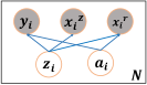
Figure 1: Probabilistic Graphical Model of FairWS

Specifically, we assume that each data sample $(x_{i}^{z},x_{i}^{r},y_{i})$ is sampled from a generative process as shown in Figure 1, where $z_{i}$ is the intrinsic latent representation which is irrelevant to sensitive attributes $s_{i}$, and $a_{i}$ is the latent representation of sensitive attribute $s_{i}$. $x_{i}^{r}$ is dependent on sensitive attribute’s latent representation $a_{i}$ as $x_{i}^{r}$ is relevant with $s_{i}$. We assume that $y_{i}$ is also dependent on $a_{i}$ because otherwise, the data doesn’t contain bias. Since $z_{i}$ contains the intrinsic characteristic of data sample $i$, the class label $y_{i}$ is dependent on $z_{i}$. Note that $x_{i}^{r}$ is also dependent on the $z_{i}$ because $x_{i}^{r}$ also contains some information that is irrelevant to sensitive attributes. We disentangle $a_{i}$ and $z_{i}$ so that $a_{i}$ and $z_{i}$ can extract sensitive attribute information and non-sensitive information from $x_{i}^{r}$, respectively.

Following the probabilistic graphical model in Fig 1, since $x_{i}^{z}$ is irrelevant to the latent representation of sensitive attributes $a_{i}$, and $x_{i}^{r}$ is highly correlated with $z_{i}$, the joint distribution can be written as:

$$p\left(a_{i},y_{i},z_{i},x_{i}^{r},x_{i}^{z}\right)=$$ (1)

$$p\left(a_{i}\right)p\left(z_{i}\right)p\left(x_{i}^{r}\mid a_{i},z_{i}\right)p\left(x_{i}^{z}\mid z_{i}\right)p\left(y_{i}\mid z_{i},a_{i}\right)$$

where $p(a_{i})$ and $p(z_{i})$ are the prior distributions. Our goal is to maximize the likelihood of the joint distribution of observed variables, i.e., $p_{\theta}(x_{i}^{r},x_{i}^{z},y_{i})$. However, directly maximizing it is difficult as it contains latent variables $z_{i}$ and $a_{i}$. Following VAEs Kingma and Welling (2013) , we maximize the variational lower bound of this likelihood as:

$$\log p_{\theta}(x_{i}^{r},x_{i}^{z},y_{i})\geq$$ (2)

$$\mathbb{E}_{q_{\phi}(a_{i},z_{i}\mid x_{i}^{z},x_{i}^{r},y_{i})}\left[p_{\theta}\left(x_{i}^{r},x_{i}^{z},y_{i}\mid z_{i},a_{i}\right)\right]$$

$$-D_{KL}\left(q_{\phi}\left(a_{i},z_{i}\mid x_{i}^{z},x_{i}^{r},y_{i}\right)\|p\left(z_{i},a_{i}\right)\right)$$

where $\mathbb{E}$ denotes the expectation, $q_{\phi}\left(a_{i},z_{i}\mid x_{i}^{z},x_{i}^{r},y_{i}\right)$ is an auxiliary distribution to approximate $p\left(a_{i},z_{i}\mid x_{i}^{z},x_{i}^{r},y_{i}\right)$, and $D_{KL}(\cdot,\cdot)$ denotes the Kullback-Leibler divergence. We treat the posterior $q_{\phi}\left(a_{i},z_{i}\mid x_{i}^{z},x_{i}^{r},y_{i}\right)=q_{\phi}\left(a_{i}\mid x_{i}^{z},y_{i}\right)q_{\phi}\left(z_{i}\mid x_{i}^{z},x_{i}^{r},y_{i}\right)$ as an encoder which learns the latent representation $a_{i}$ and $z_{i}$ from $\left(x_{i}^{z},x_{i}^{r},y_{i}\right)$.

$p_{\theta}(x_{i}^{r},x_{i}^{z},y_{i}|z_{i},a_{i})$ can be further written as

$$p_{\theta}(x_{i}^{r},x_{i}^{z},y_{i}|z_{i},a_{i})=p_{\theta}(x_{i}^{r}|a_{i},z_{i})p_{\theta}(x_{i}^{z}|z_{i}s)p_{\theta}(y_{i}|z_{i},a_{i})$$

where $p_{\theta}\left(x_{i}^{r}\mid a_{i},z_{i}\right)$ and $p_{\theta}\left(x_{i}^{z}\mid z_{i}\right)$ are the generators to generate $x_{i}^{r}$ and $x_{i}^{z}$, respectively, and $p_{\theta}\left(y_{i}\mid z_{i},a_{i}\right)$ can be treated as a biased classifier. Both $\theta$ and $\phi$ represents parameters for neural networks. Furthermore, assuming the latent variables $a_{i}$ and $z_{i}$ are conditionally independent and similarly for the prior $p(z_{i},a_{i})=p(z_{i})p(a_{i})$, $p(a_{i})$ and $p(z_{i})$ are both standard Gaussian distributions, and we can rewrite the KL divergence as:

$$D_{KL}\left(p_{\theta}\left(z_{i},a_{i}\mid x_{i}^{z},x_{i}^{r},y_{i}\right)\|p\left(z_{i},a_{i}\right)\right)$$ (3)

$$=D_{KL}(p_{\theta}\left(z_{i}\mid x_{i}^{z},x_{i}^{r},y_{i}\right)\|p(z_{i}))+$$

$$D_{KL}(p_{\theta}\left(a_{i}\mid x_{i}^{r},y_{i}\right)\|p(a_{i}))$$

Now we have two KL divergence terms regularizing $p_{\theta}(z_{i}|x_{i}^{z},x_{i}^{r},y_{i})$ and $p_{\theta}(a_{i}|x_{i}^{r},y_{i})$, respectively. To provide flexibility of our model, following Higgins et al. (2016), we add a weight hyperparameter $\beta$ to control the influence of $D_{KL}(p_{\theta}\left(a_{i}\mid x_{i}^{r},y_{i}\right)\|p(a_{i}))$. Then the variational lower bound can be written as

$$\mathcal{L}^{i}_{ELBO} =\mathbb{E}_{\left.q_{\phi}(a_{i},z_{i}\mid x_{i}^{z},x_{i}^{r},y_{i}\right)}\left[p_{\theta}\left(x_{i}^{r},x_{i}^{z},y_{i}\mid z_{i},a_{i}\right)\right]$$ (4)

$$-D_{KL}(p_{\theta}\left(z_{i}\mid x_{i}^{z},x_{i}^{r},y_{i}\right)\|p(z_{i}))$$

$$-\beta D_{KL}(p_{\theta}\left(a_{i}\mid x_{i}^{r},y_{i}\right)\|p(a_{i}))$$

An illustration of sensitive attribute estimation framework is shown in the right part of Fig. LABEL:Fig2, where each term can be implemented as a neural network. To facilitate efficient large-scale training, we adopt reparameterization trick Kingma and Welling (2013). Since both $z_{i}$ and $a_{i}$ are dependent on the relevant features $X^{r}$, to make sure that $z_{i}$ and $a_{i}$ are disentangled, i.e., $z_{i}$ captures the class label related information from $x_{i}^{r}$ while $z_{i}$ captures sensitive attribute related information, we add a regularizer to minimize the mutual information between $z_{i}$ and $a_{i}$, i.e.,

$$\min_{\theta,\phi}~{}I(A;Z)=h(A)-h(A\mid Z)$$ (5)

where $A$ is a matrix with the $i$-th row as $a_{i}$ and $Z$ is a matrix with the $i$-th row as $z_{i}$. $h(\cdot)$ denotes the entropy function and $I(A,Z)$ measures dependencies between $A$ and $Z$. However, the mutual information $I(A;Z)$ is difficult to calculate directly. We follow Belghazi et al. (2018) to efficiently estimate the mutual information. The basic idea is to train a classifier $D$ to distinguish between sample pairs from the joint distribution $P(a_{i},z_{i})$ and $P(a_{i})P(z_{i})$ and approximate the mutual information as:

$$I(A;Z) \approx\mathbb{E}_{P(a_{i},z_{i})}[\mathcal{D}(a_{i},z_{i})]-\log\mathbb{E}_{P(a_{i})P(z_{i})}\left[e^{\mathcal{D}(a_{i},z_{i})}\right]$$ (6)

$$=\mathcal{L}_{MI}$$

where $D(a_{i},z_{i})$ is a binary discriminator judging if $(a_{i},z_{i})$ is from $P(a_{i},z_{i})$ or $P(a_{i})P(z_{i})$. The final objective function of our sensitive attributes estimation module is:

$$\min_{\theta,\phi}\frac{1}{N}\sum_{i=1}^{N}-\mathcal{L}^{i}_{ELBO}+\mathcal{L}_{MI}$$ (7)

Once the model is trained, we can estimate each data sample $i$’s latent representation of sensitive attributes by sampling from $q_{\phi}\left(a_{i}\mid x_{i}^{z},y_{i}\right)$.

4.2 Fairness Regularization

As shown in Figure LABEL:Fig2, we can obtain $i$-th data sample’s latent representation of sensitive attributes, $a_{i}$, from the sensitive attributes estimation part. Then, the second step is to use sampled $a_{i}$ to regularize a base classifier to learn a fair classifier. One way to make the prediction fair is to reduce the correlation between the prediction and the sensitive attribute $s_{i}$. Since $a_{i}$ is the latent representation of $s_{i}$, the regularization form can be the correlation between predicted label vectors and latent sensitive attributes vectors, which is given as:

$$\mathcal{L}_{\text{reg}}=\sum_{k=1}^{d}\sum_{j=1}^{m}\left|\sum_{i=1}^{N}\left(y^{\prime}_{ij}-\bar{y}_{j}^{\prime}\right)\left(a_{ik}-\bar{a}_{k}\right)\right|$$ (8)

where $N$ is the number of samples and $m$ is the number of class. $d$ is the dimension of $a_{i}$ and $a_{ik}$ is the $k$-th element of $a_{i}$. $\bar{a}_{k}=\frac{1}{N}\sum_{i=1}^{N}a_{ik}$. $y^{\prime}_{ij}$ denotes the predicted probability of class $j$ for sample $i$, $\bar{y}^{\prime}_{j}=\frac{1}{N}\sum_{i=1}^{N}y_{ij}$. To predict $y_{i}^{\prime}$ for the sample $i$, we utilize the following function:

$$y_{i}^{\prime}=g_{w_{1}}(x_{i}^{z}\oplus f_{w_{2}}(x_{i}^{r}))$$ (9)

where $\oplus$ is the concatenation operator of two vectors, $g_{w_{1}}(\cdot)$ represent multi-layered perceptrons (MLPs), $f_{w_{2}}(\cdot)$ is utilized to transform $x_{i}^{r}$ to a vector if $x_{i}^{r}$ represents a review or social interactions, $w_{1}$ and $w_{2}$ are both trainable parameters of neural networks. Note that $f(x_{i}^{r})=x_{i}^{r}$ if $x_{i}^{r}$ is a relevant feature vector of the sample $i$. Also, the classifier $g_{w}$ also has a loss for the label prediction and it can be denoted as $L_{clf}$. $L_{clf}$ is the cross-entropy loss in our experiment setting. The final objective function of FairWS is given as:

$$\min_{w_{1},w_{2}}\mathcal{L}_{clf}+\lambda\mathcal{L}_{reg}$$ (10)

where $\lambda$ is a scalar controlling the trade-off between the accuracy and fairness.

5 Experiments

In this section, we conduct extensive experiments to evaluate the effectiveness of the proposed framework. In particular, we aim to answer the following research questions:

• (RQ1) How does the proposed FairWS perform in terms of both classification accuracy and fairness?

• (RQ2) How accurate is the proposed framework in estimating sensitive attributes?

• (RQ3) How does the quality of sensitive attributes affect the performance of FairWS?

Table 1: Comparison of different approaches in three datasets.

	Adult			Credit Defaulter			Animate
Methods	ACC	$\Delta_{EO}$	$\Delta_{DP}$	ACC	$\Delta_{EO}$	$\Delta_{DP}$	ACC	$\Delta_{EO}$	$\Delta_{DP}$
Vanilla	0.856 $\pm$ 0.001	0.046 $\pm$ 0.006	0.089 $\pm$ 0.005	0.731 $\pm$ 0.001	0.159 $\pm$ 0.001	0.101 $\pm$ 0.001	0.755 $\pm$ 0.001	0.330 $\pm$ 0.001	0.391 $\pm$ 0.001
ConstrainS	0.845 $\pm$ 0.002	0.040 $\pm$ 0.003	0.058 $\pm$ 0.004	0.713 $\pm$ 0.006	0.137 $\pm$ 0.002	0.087 $\pm$ 0.003	0.738 $\pm$ 0.008	0.202 $\pm$ 0.005	0.264 $\pm$ 0.003
ARL	0.861 $\pm$ 0.003	0.034 $\pm$ 0.012	0.141 $\pm$ 0.008	0.578 $\pm$ 0.001	0.050 $\pm$ 0.005	0.054 $\pm$ 0.009	0.688 $\pm$ 0.002	0.241 $\pm$ 0.003	0.132 $\pm$ 0.002
KSMOTE	0.560 $\pm$ 0.002	0.141 $\pm$ 0.031	0.012 $\pm$ 0.022	0.563 $\pm$ 0.003	0.203 $\pm$ 0.002	0.258 $\pm$ 0.001	0.672 $\pm$ 0.004	0.174 $\pm$ 0.001	0.320 $\pm$ 0.002
RemoveR	0.801 $\pm$ 0.010	0.124 $\pm$ 0.004	0.071 $\pm$ 0.002	0.576 $\pm$ 0.002	0.028 $\pm$ 0.001	0.041 $\pm$ 0.003	0.699 $\pm$ 0.001	0.106 $\pm$ 0.004	0.197 $\pm$ 0.002
ConstrainR	0.832 $\pm$ 0.013	0.061 $\pm$ 0.015	0.088 $\pm$ 0.019	0.668 $\pm$ 0.014	0.121 $\pm$ 0.012	0.081 $\pm$ 0.016	0.726 $\pm$ 0.017	0.257 $\pm$ 0.010	0.329 $\pm$ 0.012
FairRF	0.832 $\pm$ 0.001	0.025 $\pm$ 0.009	0.066 $\pm$ 0.004	0.561 $\pm$ 0.003	0.008 $\pm$ 0.002	0.008 $\pm$ 0.001	0.555 $\pm$ 0.001	0.021 $\pm$ 0.002	0.010 $\pm$ 0.001
FairWS	0.842 $\pm$ 0.004	0.024 $\pm$ 0.012	0.054 $\pm$ 0.010	0.720 $\pm$ 0.012	0.145 $\pm$ 0.016	0.087 $\pm$ 0.010	0.726 $\pm$ 0.016	0.173$\pm$ 0.014	0.247 $\pm$ 0.016
FairWS + MI	0.833 $\pm$ 0.006	0.013$\pm$ 0.011	0.046 $\pm$ 0.019	0.719 $\pm$ 0.028	0.145 $\pm$ 0.019	0.074 $\pm$ 0.011	0.732 $\pm$ 0.020	0.178$\pm$ 0.016	0.263 $\pm$ 0.012

5.1 Datasets

We conduct experiments on three publicly available benchmark datasets, including Adult Asuncion and Newman (2007), Credit Defaulter Dong et al. (2021) and Animate. The statistics of datasets are summarized in Appendix.

• Adult: This dataset contains records of personal yearly income. The task is to predict whether the yearly salary is over or under $50 and the sensitive attribute is gender. It has 12 features. We use age, relation, and marital status as relevant features $X^{r}$ and the rest as non-relevant features.

• Credit Defaulter: In the Credit Defaulter dataset, each data sample is a person which has 14 features about their personal information. In addition, two samples are connected based on the similarity of their purchase and payment records, which forms a graph. The sensitive attribute of this dataset is age and the task is to classify whether a user is married. Each person’s connectivity is treated as relevant features $X^{r}$ because it is relevant to age, i.e., two persons of similar age are more likely to be connected and have similar connectivity.

• Animate: This dataset includes records of users’ reviews and their personal profiles. The task is to predict whether the average ranking of users’ favorite movies is in the top 400 and the sensitive attribute is whether the average scores the users give to their favorite movies are above 8. Note that the ranking of movies is evaluated from website Animate based on their popularity and rating scores. We treat the text review from users as relevant features $X^{r}$ and their personal attributes as irrelevant features. Text reviews are also important relevant features because reviews can represent people’s attitudes to the movie, i.e. whether to give this movie a higher score and also their occupations, age or other sensitive information.

For Adult and Animate, We make the train:eval:test split ratio as 5 : 2.5 : 2.5. For Credit Defaulter, following Dong et al. (2021), we select 2000 nodes as the training set, 25% for validation, 25% for testing.

5.2 Experimental Setup

Baselines. To evaluate the effectiveness of FairWS, we it compare with the vanilla model, sensitive-attribute-aware model and fair models without sensitive attributes.

• Vanilla: It utilizes the base classifier without the regularization form. The base classifier $g_{w_{1}}(\cdot)$ is MLPs for all dataset. The transform model $f_{w_{2}}(\cdot)$ is Graph Convolutional Network (GCN) Kipf and Welling (2016) for dataset Credit Defaulter, Convolutional Neural Network (CNN) Lawrence et al. (1997) for dataset Animate.

• ConstrainS: We assume the sensitive attribute of each sample is known for this baseline. We add the correlation regularizer between sensitive attributes and the model output to the original loss of the Vanilla model. ConstrainS aims at showing the accuracy and fairness we can achieve, which is the upper bound for the proposed methods.

• Models without Sensitive Attributes: KMeans SMOTE Yan et al. (2020) conduct clustering and treat clustering groups as pseudo sensitive attributes to achieve fairness. RemoveR Zhao et al. (2021) remove all candidate-relevant features for fair classifiers. ConstrainR calculates the correlation regularization form on relevant features. ARL Lahoti et al. (2020) optimizes the model’s performance through reweighting under-represented regions detected by an adversarial model, which can alleviate bias. FairRF Zhao et al. (2021) uses relevant features to regularize the model to be fair.

For baselines such as FairRF and ConstrainR, since the graph and text cannot be directly utilized to regularize the model, we adopt Node2vec Grover and Leskovec (2016) to obtain the node embeddings as relevant features on Credit Defaulter. For Animate, $X^{r}$ are texts and we utilize the average of the pretrained word embeddings as relevant feature vectors for ConstrainR and FairRF.

Configurations. For ARL and KSMOTE Lahoti et al. (2020); Yan et al. (2020), we utilize the authors’ codes. For other baselines, we follow Zhao et al. (2021)’s implementations. For the decoder and encoder of our sensitive estimation module, we implement a multi-layer perceptron (MLP) network with two and three layers, respectively. The hidden dimension is 8 for the Adult dataset, 50 for the graph dataset, 16 for the text dataset. For classifier $g_{w_{1}}(\cdot)$, we adopt three-layer MLPs for the adult dataset and one-layer for other datasets. We implement two-layer GCN and CNN for graph and text datasets separately. Adam optimizer is adopted to train the model, with an initial learning rate of 0.001 for all datasets.

Evaluation Metrics We use accuracy as a metric for the classification problem. Following existing work on fair models  Mehrabi et al. (2021), we adopt equal opportunity $\Delta_{EO}$ and demographic parity $\Delta_{DP}$ as the fairness metrics. The smaller $\Delta_{EO}$ and $\Delta_{DP}$ are, the more fair the model is. The details of fairness metrics are given in the Appendix.

5.3 Experimental Results

To answer RQ1, we conduct each experiment 5 times and report the average results along with standard deviation in terms of accuracy, $\Delta_{EO}$ and $\Delta_{DP}$ on three datasets in Table 1. Note that FairWS + MI means that we utilize the mutual information loss for the sensitive attributes estimation module and FairWS means no mutual information loss. For all baselines, the hyperparameters are tuned via grid search on the validation dataset. Specific hyperparameters for both FairWS and FairWS + MI are put into the Appendix. From the Table 1, we make the following observations:

• Comparing Vanilla with ConstrainR, we can observe that directly constraining relevant features $X^{r}$ can help the model achieve fairer results on Adult, which is because $X^{r}$ of Adult are simple features that can be easily incorporated into the covariance regularizer. However, when $X^{r}$ is complex features such as text on Animate and graph on Credit Defaulter, ConstrainR method doesn’t have too much effect, which is because the learned embedding vectors obtained from an unsupervised manner, which are treated as relevant features, may be irrelevant to the targeted sensitive attributes. While for FairWS, it can extract the targeted sensitive information from the graph structure or text reviews flexibly via Variational Autoencoders in the sensitive attributes estimation part.

• Compared with baselines without the sensitive attributes, FairWS can achieve the best result in terms of the accuracy and fairness metrics. Even though ARL can achieve fairer performance, it will result in a significant drop in accuracy. Also, FairRF can improve the fairness performance on the Adult dataset as shown in Table  1, but it can’t work on the graph and text dataset.

• In comparison with ConstrainS, we can achieve comparable performance or even better performance with a little drop in accuracy for all datasets. And our proposed mutual information loss can help the fairness regularization form get better performance on the Adult dataset. In addition, it can result in comparable results on fairness metrics with higher accuracy for the text and graph dataset.

To answer RQ2, we conduct an experiment to show whether our generated latent representation $A$ learns information about sensitive attributes. Specifically, Gaussian Mixture Model is utilized to cluster data into two groups based on $A$ for FairWS and FairWS + MI. Then, we calculate AUC score between predicted groups and ground truth and the result is shown in Table 2, where Gaussian Mixture in the table means using Gaussian Mixture Model on raw related feature vectors. Note that this is an unsupervised setting and we evaluate the performance on the training set. From the table, we find that (i) we can obtain a large improvement compared with Gaussian Mixture on features; and (ii) it also shows that mutual information loss can help $A$ learn more information about sensitive attributes. For example, Fair + WS achieves higher AUC values on the Adult and Animate dataset.

Table 2: Comparison of different approaches for sensitive attributes estimation on three dataset.

Models	Adult	Credit Defaulter	Animate
	AUC	AUC	AUC
FairWS	0.7616	0.7250	0.7884
FairWS + MI	0.7724	0.7134	0.7930
Gaussian Mixture	0.5087	0.5238	0.5363

5.4 Hyperparameter Sensitivity Analysis

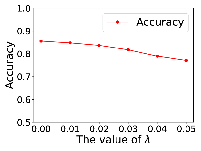
(a) Accuracy

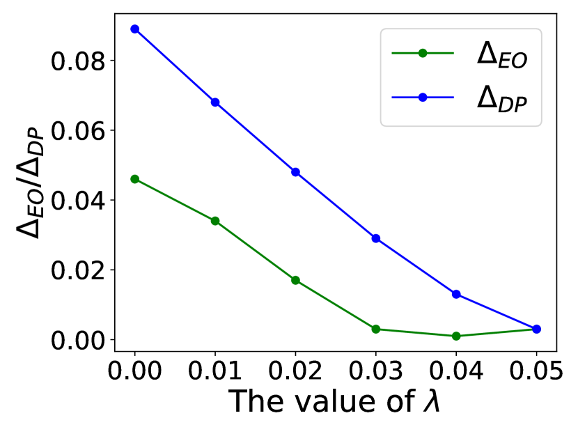
(b) $\Delta_{EO}$ and $\Delta_{DP}$

Figure 3: Test accuracy and $\Delta_{EO}$ and $\Delta_{DP}$ w.r.t. the hyperparameter $\lambda$ on the dataset Adult.

The proposed FairWS has two important hyperparameters $\lambda$ and $\beta$. $\lambda$ controls the trade-off between fairness and accuracy when learning the fair classifier. To evaluate the parameter sensitivity on $\lambda$, we fix the sensitive attributes estimation module with $\beta=0.01$ and train a fair classifier based on the generated latent representation with different $\lambda$. $\lambda$ is varied as $\{0,0.01,0.02,0.03,0.04,0.05\}$. Figure 3 shows the results on Adult dataset. From Figure 3, we can observe that larger $\lambda$ will lead to worse performance on accuracy and better performance on $\Delta_{EO}$ and $\Delta_{DP}$, which is because higher weight of correlation loss between predicted results and sensitive information will lead to a fairer model but with a drop of accuracy. Thus, it’s important to select a $\lambda$ for various requirements e.g. better performance on accuracy or fairness metrics.

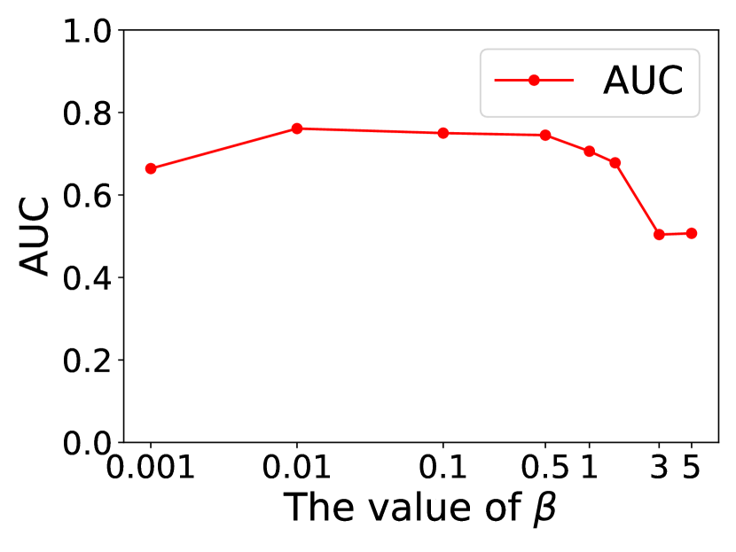
(a) Adult

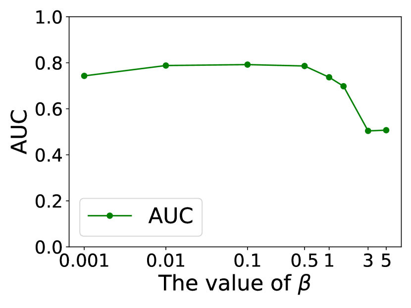
(b) Animate

Figure 4: Sensitivity of $\beta$ on sensitive attribute estimation.

Another hyperparameter $\beta$ is to control the training process of the latent representation $A$. We vary $\beta$ as $\{0.001,0.01,0.1,0.5,1,1.5,3,5\}$. For each choice of $\beta$, we learn $A$ and use Gaussian Mixture Model to predict the sensitive attributes from $A$. The results of sensitive attribute estimation in terms of AUC are shown in Fig. 4. We observe that the performance first increases when $\beta$ increase from 0.001 to 0.01, and then results tend to be fluent. Finally, when $\beta$ is larger than 1, the AUC values drop to 0.5. Therefore, small and large $\beta$ will result in less sensitive information in $A$ and the best value of it is between 0.01 to 0.5.

5.5 Impact of Relevant Features

Table 3: AUC values for the impact of relevant features on Adult.

Methods	Random	Top-1	Noisy	GM	FairWS
AUC	0.6681	0.6678	0.7019	0.5078	0.7616

To answer RQ3, we explore the impact of relevant features on FiarWS and the results are shown in Table 3. Note that we choose to evaluate the quality of $A$ so we follow the experiments in Table 2 with different relevant features. In Table 3, Random means that we randomly select features as relevant features. Top-1 uses the most-effective relevant feature, i.e., we report the one that achieves the highest performance when treated as relevant features. Noisy randomly replaces one attribute in the original $X^{r}$ with irrelevant ones. GM follows Table 2 to obtain the protected groups via Gaussian Mixture Model on the raw relevant features. Note that Random, Noisy and GM all utilize three relevant features. Hyperparameters for all these methods are found via grid search, and the experiments are conducted 5 times. All these methods are trained on the FairWS model with different relevant features. We can observe that FairwS can also learn information about the sensitive attributes even with the noisy relevant features. Comparing FairWS with Top-1, we can find that sensitive information in one feature is limited but FairWS can utilize a set of relevant features to learn sensitive information automatically and achieve great performance.

6 Conclusion

In this paper, we study a novel problem of training fair and accurate classifiers without sensitive attributes by estimating sensitive information from non-sensitive features. We propose a novel framework FairWS which learns sensitive information from relevant features and regularizes classifiers based on inferred sensitive information. FairWS can flexibly learn sensitive information from relevant features in different formats and from noisy relevant features. Through extensive experiments, we demonstrate that our method significantly outperformed the state-of-the-art methods w.r.t both accuracy and fairness metrics when sensitive attributes are unavailable.

Appendix A Appendix

A.1 Hyperparameter for FairWS

The hyperparameters to reproduce the result in Table 1 are shown in this section. For the dataset Adult, we set $\lambda=0.017$, $\beta=0.01$ for FairWS, $\lambda=0.01$, $\beta=0.01$ for FairWS + MI. For the dataset Animate, we set $\lambda=0.042$, $\beta=0.01$ for FairWS, $\lambda=0.033$, $\beta=0.01$ for FairWS + MI. For the dataset Credit Defaulter, we set $\lambda=0.012$, $\beta=0.07$ for FairWS, $\lambda=0.00042$, $\beta=0.01$ for FairWS + MI. Note that the hyperparamters can achieve the results shown in this paper and a large set of other hyperparamters can also obtain the similar results.

A.2 Fairness metrics

To measure the fairness, we adopt two widely used evaluation metrics like equal opportunity and demographic parity, and it’s defined as follows:

Equal Opportunity Mehrabi et al. [2021]: Equal Opportunity requires that the model assigns the equal probability of positive instances with random protected attributes $i$, $j$ to a data point with a positive label. In this paper, we report the difference for equal opportunity ($\Delta EO$):

$$\Delta_{EO}=|\mathbb{E}(y^{\prime}\mid S=i,y=1)-\mathbb{E}(y^{\prime}\mid S=j,y=1)|$$ (11)

, where $y^{\prime}$ is the output of the model $g_{w_{2}}$, $S$ represents the sensitive attributes. Note that the tasks in our experiment are binary classification problems so $y^{\prime}$ means the probability to be predicted as positive labels.

Demographic Parity Mehrabi et al. [2021]: Demographic Parity requires that the predicted results of models are fair on different sensitive groups. We also report the difference in Demographic Parity in this paper:

$$\Delta_{DP}=|\mathbb{E}(y^{\prime}\mid S=i)-\mathbb{E}(y^{\prime}\mid S=j)|$$ (12)

, and lower $\Delta_{EO}$ and $\Delta_{DP}$ represent the fairer model.

A.3 Statistics of Datset

We put the dataset statistics into this section, the table includes the number of features for each dataset, the number of class labels, the formats of their relevant features and the number of data samples. Note that the personal attributes represent the feature vectors which can represent the characteristics of people.

Table 4: Statistics of Datset.

Dataset	Adult	Credit Defaulter	Animate
Features	12	13	15
Class	2	2	2
Type of $X^{r}$	Personal Attributes	Graph	Text
Data Size	45,211	30,000	12,772

References

- Asuncion and Newman [2007] Arthur Asuncion and David Newman. Uci machine learning repository, 2007.
- Belghazi et al. [2018] Mohamed Ishmael Belghazi, Aristide Baratin, Sai Rajeswar, Sherjil Ozair, Yoshua Bengio, Aaron Courville, and R Devon Hjelm. Mine: mutual information neural estimation. arXiv preprint arXiv:1801.04062, 2018.
- Beutel et al. [2017] Alex Beutel, Jilin Chen, Zhe Zhao, and Ed H Chi. Data decisions and theoretical implications when adversarially learning fair representations. arXiv preprint arXiv:1707.00075, 2017.
- Coston et al. [2019] Amanda Coston, Karthikeyan Natesan Ramamurthy, Dennis Wei, Kush R Varshney, Skyler Speakman, Zairah Mustahsan, and Supriyo Chakraborty. Fair transfer learning with missing protected attributes. In Proceedings of the 2019 AAAI/ACM Conference on AI, Ethics, and Society, pages 91–98, 2019.
- Dong et al. [2021] Yushun Dong, Ninghao Liu, Brian Jalaian, and Jundong Li. Edits: Modeling and mitigating data bias for graph neural networks. arXiv preprint arXiv:2108.05233, 2021.
- Dwork et al. [2012] Cynthia Dwork, Moritz Hardt, Toniann Pitassi, Omer Reingold, and Richard Zemel. Fairness through awareness. In Proceedings of the 3rd innovations in theoretical computer science conference, 2012.
- Feldman et al. [2015] Michael Feldman, Sorelle A Friedler, John Moeller, Carlos Scheidegger, and Suresh Venkatasubramanian. Certifying and removing disparate impact. In proceedings of the 21th ACM SIGKDD international conference on knowledge discovery and data mining, pages 259–268, 2015.
- Grover and Leskovec [2016] Aditya Grover and Jure Leskovec. node2vec: Scalable feature learning for networks. In Proceedings of the 22nd ACM SIGKDD international conference on Knowledge discovery and data mining, pages 855–864, 2016.
- Hardt et al. [2016] Moritz Hardt, Eric Price, and Nati Srebro. Equality of opportunity in supervised learning. Advances in neural information processing systems, 29:3315–3323, 2016.
- Higgins et al. [2016] Irina Higgins, Loic Matthey, Arka Pal, Christopher Burgess, Xavier Glorot, Matthew Botvinick, Shakir Mohamed, and Alexander Lerchner. beta-vae: Learning basic visual concepts with a constrained variational framework. 2016.
- Kingma and Welling [2013] Diederik P Kingma and Max Welling. Auto-encoding variational bayes. arXiv preprint arXiv:1312.6114, 2013.
- Kipf and Welling [2016] Thomas N Kipf and Max Welling. Semi-supervised classification with graph convolutional networks. arXiv preprint arXiv:1609.02907, 2016.
- Lahoti et al. [2020] Preethi Lahoti, Alex Beutel, Jilin Chen, Kang Lee, Flavien Prost, Nithum Thain, Xuezhi Wang, and Ed H Chi. Fairness without demographics through adversarially reweighted learning. arXiv preprint arXiv:2006.13114, 2020.
- Lawrence et al. [1997] Steve Lawrence, C Lee Giles, Ah Chung Tsoi, and Andrew D Back. Face recognition: A convolutional neural-network approach. IEEE transactions on neural networks, 8(1):98–113, 1997.
- Locatello et al. [2019] Francesco Locatello, Gabriele Abbati, Tom Rainforth, Stefan Bauer, Bernhard Schölkopf, and Olivier Bachem. On the fairness of disentangled representations. arXiv preprint arXiv:1905.13662, 2019.
- Mehrabi et al. [2021] Ninareh Mehrabi, Fred Morstatter, Nripsuta Saxena, Kristina Lerman, and Aram Galstyan. A survey on bias and fairness in machine learning. ACM Computing Surveys (CSUR), 54(6):1–35, 2021.
- Otterbacher [2010] Jahna Otterbacher. Inferring gender of movie reviewers: exploiting writing style, content and metadata. In Proceedings of the 19th ACM international conference on Information and knowledge management, pages 369–378, 2010.
- Pleiss et al. [2017] Geoff Pleiss, Manish Raghavan, Felix Wu, Jon M Kleinberg, and Kilian Q Weinberger. On fairness and calibration. In NIPS, 2017.
- Wang et al. [2016] Pengfei Wang, Jiafeng Guo, Yanyan Lan, Jun Xu, and Xueqi Cheng. Multi-task representation learning for demographic prediction. In European Conference on Information Retrieval, pages 88–99. Springer, 2016.
- Xu et al. [2018] Depeng Xu, Shuhan Yuan, Lu Zhang, and Xintao Wu. Fairgan: Fairness-aware generative adversarial networks. In 2018 IEEE International Conference on Big Data (Big Data), pages 570–575. IEEE, 2018.
- Yan et al. [2020] Shen Yan, Hsien-te Kao, and Emilio Ferrara. Fair class balancing: enhancing model fairness without observing sensitive attributes. In Proceedings of the 29th ACM International Conference on Information & Knowledge Management, pages 1715–1724, 2020.
- Zafar et al. [2017] Muhammad Bilal Zafar, Isabel Valera, Manuel Gomez Rogriguez, and Krishna P Gummadi. Fairness constraints: Mechanisms for fair classification. In Artificial Intelligence and Statistics, pages 962–970. PMLR, 2017.
- Zhang et al. [2018] Brian Hu Zhang, Blake Lemoine, and Margaret Mitchell. Mitigating unwanted biases with adversarial learning. In Proceedings of the 2018 AAAI/ACM Conference on AI, Ethics, and Society, pages 335–340, 2018.
- Zhao et al. [2021] Tianxiang Zhao, Enyan Dai, Kai Shu, and Suhang Wang. You can still achieve fairness without sensitive attributes: Exploring biases in non-sensitive features. arXiv preprint arXiv:2104.14537, 2021.