Nonadiabatic Landau-Zener-Stückelberg-Majorana transitions, dynamics, and interference

Abstract

Since the pioneering works by Landau, Zener, Stückelberg, and Majorana (LZSM), it has been known that driving a quantum two-level system results in tunneling between its states. Even though the interference between these transitions is known to be important, it is only recently that it became both accessible, controllable, and useful for manipulating a growing number of quantum systems. Here, we study systematically various aspects of LZSM physics and review the relevant literature, significantly expanding the review article in Ref. Shevchenko et al. (2010).

Abbreviations and most-often-used symbols:

For the readers’ convenience, below we list the main abbreviations used in this work. This list also includes some of the topics covered.

AIM:    adiabatic-impulse model;

CDT:   coherent destruction of tunneling;

JJ:        Josephson junction;

KZM:  Kibble-Zurek mechanism;

LZSM: Landau-Zener-Stückelberg-Majorana;

PAT:     photon-assisted tunneling;

RAP:   rapid adiabatic passage;

RWA:   rotating-wave approximation;

TLS:     two-level system;

TM:      transfer matrix.

——————————

$\mathcal{P}$: single-passage LZSM transition probability;

$\Delta$: minimal energy-level splitting;

$\varepsilon$: energy bias;

$A,\omega,T_{\mathrm{d}}$: amplitude, frequency, and period of the driving field;

$\delta$: adiabaticity parameter;

$\Delta E$: qubit energy-level gap;

$\Gamma_{1,2}=T_{1,2}^{-1}$: relaxation and decoherence rates;

$T$: temperature.

“Without nonadiabatic transition, this world would have been dead, because no basic chemical and biological processes, such as electron and proton transfer, could have occurred. Nonadiabatic transition is certainly an origin of mutability of this world.” 

Zhu et al. (2007)

I Introduction

The quantum two-level system (TLS) is one of the basic models in quantum physics and describes systems that are ubiquitous in nature. On the one hand, this is the “simplest nonsimple quantum problem”, quoting Berry (1995); and, on the other hand, this provides the basis for quantum technologies, in which a TLS refers to a qubit.

If a quantum system is excited by a time-dependent drive, it displays a variety of interesting and important effects. Note that several Nobel Prizes in physics have been awarded to physicists who exploited time-dependent few-level quantum systems:

• 1944: Rabi on molecular beams and nuclear magnetic resonance;

• 1952: Bloch and Purcell on magnetic fields in atomic nuclei and nuclear magnetic moments;

• 1964: Townes, Basov, and Prochorov on masers, lasers, and quantum optics;

• 1966: Kastler on optical pumping;

• 1989: Ramsey, Dehmelt, and Paul on atomic spectroscopy, hydrogen maser, and atomic clocks;

• 1997: Chu, Cohen-Tannoudji, and Philips on cooling and trapping atoms with laser light;

• 2012: Haroche and Wineland on coupled atoms and photons;

• 2022: Aspect, Clauser, and Zeilinger on entangled photons and quantum information science.

I.1 Relation to previous work and structure of this paper

We could ask ourselves a question here, quoting Ref. Benderskii et al. (2003):

“The title of this paper might sound perplexing at first sight. What else can be said about the Landau–Zener (LZ) problem after the numerous descriptions in both research and textbook literature?”

Below we give several reasons, starting from the fact that this topic should be called LZSM, not only LZ, and ending with the point that this evergreen topic is nowadays important for many areas of physics and its applications are growing over time.

LZSM transitions are ubiquitous and important and have been addressed in several review articles (e.g., Kazantsev et al. (1985); Shimshoni and Gefen (1991); Grifoni and Hänggi (1998); Zhu et al. (2007); Shevchenko et al. (2010); Dziarmaga (2010); Silveri et al. (2017); Sen et al. (2021)) and books Nakamura (2012); Shevchenko (2019); Nakamura (2019). In particular, the central idea of a previous review Ref. Shevchenko et al. (2010) was a detailed presentation of the theoretical description of periodically driven TLSs. Here, we briefly mention the key aspects where the present work significantly extends this previous one:

• We show how to derive the LZSM formula by following the original works and not only presenting the readers these often-cited and difficult-to-access works. We also convincingly demonstrate that what is known as Zener or Landau-Zener transition/formula should be attributed to the four physicists: Landau, Zener, Stückelberg, and Majorana (LZSM).

• We address different important aspects of the nonadiabatic transition, such as transition time, nonlinearity, and dissipation.

• We relate the LZSM formalism for avoided-level crossing with the Kibble–Zurek mechanism (KZM), which has been widely used to describe second-order phase transitions.

• We review new results that have appeared in the decade following the previous review article Shevchenko et al. (2010) and also cover various physical realizations.

• We emphasize that the detailed understanding of LZSM dynamics and its aspects, such as multi-photon transitions, is important not only for spectroscopy or interferometry, but also for quantum control.

For example, the original LZSM problem was covered very briefly in Giacomo and Nikitin (2005). However, we must ask what was studied in the original works of LZSM. Many (probably, the vast majority of) researchers cite the original works by LZSM without seeing those papers, which are difficult to access and read. Moreover, out of those five papers Landau (1932a, b); Zener (1932); Stückelberg (1932); Majorana (1932), only one Zener (1932) was written in English. [See the translations in Refs. Haar (1965); Stueckelberg (1970); Cifarelli (2020a).] One of the tasks in the current review article is to present a pedagogical summary of these original works of LZSM. We believe that seeing all four approaches together is both instructive and pedagogical.

The present review paper is organized as follows: First, in the rest of Sec. I, we present diverse physical systems that can effectively be described as TLSs. A nonadiabatic transition between energy levels, known as the LZSM transition, is described in Sec. II, with details provided in Appendix A. Various approaches to the description of a periodically driven TLS are the subject of Sec. III and Appendix B. We devote Sec. IV to the description of experimental studies, in which the LZSM interference is relevant. Quantum control with nonadiabatic transitions and periodic driving is outlined in Sec. V. Related classical coherent phenomena are considered in Sec. VI. Section VII presents the conclusions.

I.2 Driven few-level systems

First, we outline the systems in which the phenomena are taking place. These are very different in their physical origins because the objects can be microscopic (electron or nuclear spins, photons, atoms), mesoscopic (superconducting qubits, quantum dots, graphene structures), or macroscopic (mechanical or electrical resonators) Nakamura (2019); Kjaergaard et al. (2020). Our aim is to demonstrate that the description of all these can be reduced to a quantum two- or few-level system. Here, the key idea is to show that a basic notion in quantum mechanics—a TLS with avoided-level crossing—is ubiquitous and that for such systems, LZSM physics is relevant. We have chosen several illustrative examples and presented them in Fig. 1, with some details given in Table 1 and in the main text below.

Note that neither Fig. 1 nor Table 1 are comprehensive because neither gives a complete picture of the variety of the respective systems. The aim is to show the diversity of the systems and their characteristic parameters, including their typical sizes. A goal of this review article is to present different realizations of LZSM phenomena. In particular, the experimental realizations of the single- and multiple-passage transitions in quantum systems will be presented in Sec. II.4 and Sec. IV, respectively, while their classical counterparts will be presented in Sec. VI. After making these references to subsequent sections, we briefly describe the quantum systems. Here, a note is in order. We describe classical realizations in a separate section and otherwise consider quantum systems. Interestingly, nonadiabatic LZSM transitions are largely associated with quantum systems; and it is a rare example in physics when classical related phenomena are studied later than their quantum counterparts and not vice versa.

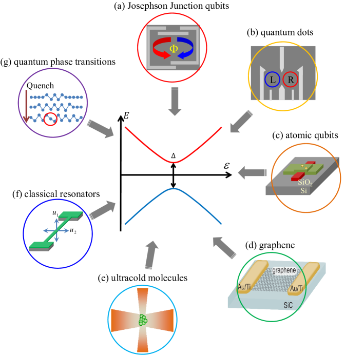
Figure 1: Various physical systems that can be described by the two-level model. These can be driven by external fields and exhibit Landau-Zener-Stückelberg-Majorana (LZSM) transitions. (a) Superconducting quantum circuits with Josephson junction (JJ) qubits are illustrated by the flux qubit, made of a superconducting ring with three tunnel JJs and the qubit states formed by the current direction (e.g., Izmalkov et al. (2004)). (b) Semiconductor artificial atoms are illustrated here by a gate-defined double quantum dot Cao et al. (2013), where the charge qubit is formed by electron states localized in either the left (L) or right (R) dot. (c) An impurity-based qubit, formed by phosphorus or arsenium donor atoms in a silicon nanowire transistor Dupont-Ferrier et al. (2013). (d) Graphene strip contacted with gold electrodes, where the current displays nonadiabatic transitions between the valence and conduction bands around the Dirac point Higuchi et al. (2017). (e) Ultracold Caesium Feshbach molecules in a laser trap, where ramping the magnetic field results in the transfer of molecular states Mark et al. (2007b). (f) Classical nanomechanical resonator Faust et al. (2012), where the coherent superposition of the in-plane and out-of-plane modes behave as a driven TLS. (g) Topological defect formation is schematically represented here by an ion Coulomb crystal; this is a trapped ion chain, where changing the confining potential results in the chain buckling; this breaking of the axial symmetry is a second-order phase transition, with the density of defects described by the Kibble-Zurek mechanism Pyka et al. (2013).

It is difficult to give a complete picture of those processes where nonadiabatic transitions between potential energy curves matter because these are ubiquitous in natural sciences. Here, we can briefly consider different physical realizations.

• As a recent example of this, in the review article Köhler et al. (2006), the role of LZSM nonadiabatic transitions is considered in the production of cold molecules and molecular association and dissociation; single and repeated nonadiabatic transitions were shown to transfer between molecular and atomic states Mark et al. (2007b); Lang et al. (2008).

• LZSM transitions become important for describing atoms being scattered by a standing light wave Kazantsev et al. (1985). The ground and excited states of an atom correspond to two effective potentials and two trajectories of motion. The possibility of nonadiabatic transitions between the two states (beams) results in changing an atom’s trajectory, which leads to interference of the translational motion states; this is similar to a two-channel optical interferometer.

• Superconducting quantum circuits are based on Josephson junctions (JJs) (see, e.g., You and Nori (2005, 2011); Xiang et al. (2013); Gu et al. (2017)). Depending on the system parameters, there are three basic types of JJ-based qubits: charge, phase, and flux ones. The energy-level spacing in these can be controlled by an external parameter: gate voltage, bias current, or magnetic flux, respectively. There are also newer subtypes, including a transmon, which is the capacitor-shunted charge qubit coupled with a transmission line; such layouts allow for better isolation from external noise, allowing for longer coherence times.

• Quantum dots with controllable parameters are mainly based on electrons that are localized in gate-defined depleted regions of semiconductor heterostructures (typically a few tens of nanometers in size), such as GaAs/AlGaAs and Si/SiGe, or in nanowire structures Zwanenburg et al. (2013). These show Coulomb blockade and display single-electron physics. Depending on which degree of freedom is relevant, we can have spin or charge qubits, which involve one or several electrons. The energy levels, including the minimal splitting, can be controlled by an external magnetic field and gate voltages.

  	System	Size	Basis	Variable	$\Delta/h$	$\omega/2\pi$	Temperature
  (a)	JJ qubits	1 $\mu$m to 1 mm	charge, current	voltage, flux	10 MHz to 10 GHz	1 GHz	50 mK
  (b)	quantum dots	10 nm to 1 $\mu$m	charge, spin	voltage, magnetic field	0.1 to 10 GHz	1 to 10 GHz	50 mK
  (c)	atomic qubits	1 Å 1 $\mu$m	electron charge or spin nuclear spin	optical and microwave fields	0.1 GHz	1 MHz to 10 GHz	50 mK to 10 K 1K to room
  (d)	graphene	1 $\mu$m	conduction bands valence bands	electric field	100 THz to 1 PHz	100 THz	room
  (e)	ultracold molecules	1 Å 40 $\mu$m	molecular states lattice bands	magnetic field lattice tilt	10 kHz	10 kHz	0.01 to 100 $\mu$K
  (f)	classical resonators	50 $\mu$m	oscillation modes	bias voltage	10 kHz	10 kHz	room
  (g)	quantum phase transitions	300 $\mu$m	defect orientation	confining voltage	100 kHz	100 kHz	$10~{}\mu$K

  Table 1: Characteristic two-level systems (TLSs) and their parameters, including minimal energy-level splitting $\Delta$ and characteristic driving frequency $\omega$. The respective systems are described in the main text, while details can be found in the references in the main text. The numbers listed above are characteristic values or ranges. The table lists both the size of the core quantum system and the size of the host. For example, for ultracold molecules, the characteristic size of the atoms is of the order of several Angstroms, while the size of the localized Bose–Einstein condensate (BEC) is typically a few dozens of micrometers.

• Atomic impurities, such as nitrogen-vacancy (NV) color centers in diamond and phosphorous impurities in silicon, allow for the manipulation of single electron spins and/or nuclear spins. These can be conveniently coupled with each other, nicely isolated from the environment, can be controlled by optical and microwave fields, and can be integrated in solid-state devices. We illustrate this with the device from Ref. Dupont-Ferrier et al. (2013), which is based on a silicon nanowire. The source-drain current was then defined by the electron transport through two tunnel-coupled donor atoms, of which the electronic-state populations created the charge qubit.

• Energy bands with avoided-level crossings, which are relevant for our consideration, also take place in graphene. When driven by an external electromagnetic field, the Dirac Hamiltonian for graphene results in LZSM phenomena near the Dirac points Higuchi et al. (2017); Heide et al. (2018). It has been shown that thin films of a Weyl semimetal subjected to a strong AC electromagnetic field should behave similarly to graphene Rodionov et al. (2016). It has also been discussed that there is a profound similarity between the effects of spatial and temporal periodicity, which is one more argument why the avoided-level-crossing structures appear in many different contexts. For a review of other related materials, the so-called “artificial graphenes”, see Montambaux (2018).

• The theory of LZSM transitions is closely related to the Kibble-Zurek mechanism (KZM) Damski (2005) which will be considered in section III.1.2. This describes second-order phase transitions, which occurs when one of the system parameters passes through a critical point. The universality of second-order phase transitions makes their dynamics independent of their microscopic nature. This results in a long list of related realizations, from cosmology to condensed matter. Leaving this intriguing issue for later, here we illustrate the realization of the KZM with chains of ions confined in harmonic traps Pyka et al. (2013). In this situation, weakening the triaxial confining potential in the transverse direction makes the chain buckle and form a zig-zag shape. This second-order phase transition can lead to the formation of topological defects, which is illustrated by a “zig”, followed by another “zig”, rather than by a “zag”. LZSM theory quantitatively describes the formation of such topological defects. Note that the characteristic parameters for defect formation in Table 1 are used for this very realization; parameters for other phase transitions may be completely different.

• Two Majorana works meet when Majorana qubits are described by the LZSM Hamiltonian. These are formed by the Majorana bound states that reside in topological superconducting systems. A realization of this could be an rf (radio frequency) superconducting quantum interference device (SQUID) with a topological JJ that is formed by a one-dimensional nanowire with spin-orbit coupling, quantum spin–Hall edge states, or ferromagnetic atomic chains You et al. (2014); Huang et al. (2015); Wang et al. (2018); Feng et al. (2018); Zhang and Liu (2021); Zhang et al. (2021). The energy level structure is controlled by an external magnetic flux. Alternatively, a topological superconductor can be a weak link between quantum dots Zazunov et al. (2020). Besides being fundamentally interesting, Majorana qubits provide the basis of topological quantum computation. For more on engineering gauge fields and triggering topological order in periodically driven systems, see Goldman and Dalibard (2014).

• Somewhat unexpectedly in this context, some classical systems can also be described as TLSs. This arises because what is needed for LZSM physics (superposition and transition between discrete states) appears not only in the quantum world, but also in classical physics. To this issue, we devote Sec. VI; but here, we illustrate this with a nanomechanical resonator in the classical regime Faust et al. (2012). This system is based on the coherent energy exchange between two strongly coupled high-quality modes of a nanomechanical resonator placed in a vacuum at ambient temperature.

• To emphasize the variety of TLSs, for which LZSM physics matters, we kaleidoscopically mention a few other realizations: electron spin-polarized ⁴He⁺ ion scattering Suzuki and Yamauchi (2010); Suzuki and Sakai (2016), low-dimensional conductors Montambaux and Jérome (2016); Benito et al. (2016), and charge-density-wave insulators Shen et al. (2014). Overall, nonadiabatic transitions are relevant in physics, chemistry, biology, economics, and some other—sometimes unexpected—research fields Nakamura (2012). As an exotic example, the LZSM model can be useful in describing decision making in which there are a few possible outcomes; in Ref. Levi (2013), the author applies the model to describe free will with afterthoughts.

II Linear drive: Landau-Zener-Stückelberg-Majorana (LZSM) transition

II.1 Hamiltonian and bases

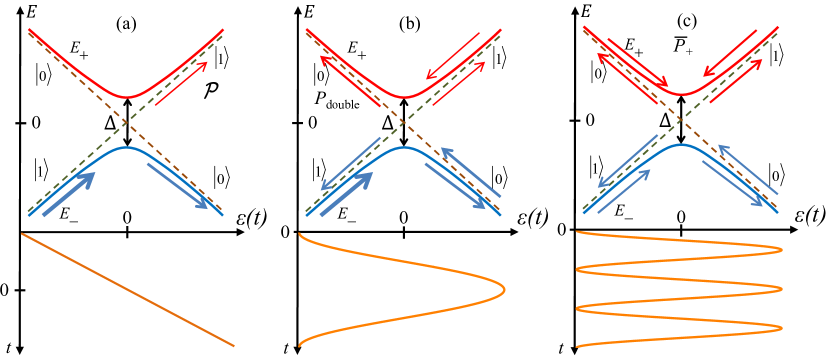
Figure 2: Schematic of a driven two-level system (TLS). Here, $E_{\pm}$ are the upper and lower energy levels, $\Delta$ is the minimal distance between energy levels, and $\varepsilon$ describes the energy bias. The avoided-crossing region corresponds to the vicinity of $\varepsilon=0$. Three problems are considered in this work: (a) single passage of the avoided-crossing region, which is described by the probability $\mathcal{P}$; (b) double-passage problem for $P_{\mathrm{double}}$; and (c) multiple-passage problem with the solution for the time-averaged probability $\overline{P}_{+}$.

We now present various approaches to derive the formula for the excitation probability of a TLS. To this end, we briefly introduce the main steps, while details are presented in Appendix A. Interestingly, this can be done in several ways within different theoretical formalisms Giacomo and Nikitin (2005). We aim to study and compare different techniques by applying these to the classical LZSM problem with a linear drive to the TLS.

Consider a TLS described by the Hamiltonian

$$\color[rgb]{1,0,0}\boxed{\color[rgb]{0,0,0}H(t)=-\frac{\Delta}{2}\sigma_{x}-\frac{\varepsilon(t)}{2}\sigma_{z}=-\frac{1}{2}\left(\begin{array}[]{cc}\varepsilon&\Delta\\ \Delta&-\varepsilon\end{array}\right),\color[rgb]{1,0,0}}\color[rgb]{0,0,0}$$ (1)

with the linear bias

$$\varepsilon(t)=vt,$$ (2)

$\Delta$ being a time-independent quantity and time $t\in(-\infty,\infty)$. Let us now define the diabatic states, which are the Hamiltonian eigenfunctions at $\Delta=0$: $\left|0\right\rangle=\binom{1}{0}$ and $\left|1\right\rangle=\binom{0}{1}$. The respective (diabatic) energy levels are $E_{0,1}=\mp\varepsilon/2$. These are plotted by the dashed lines in Fig. 2. In general, the wave function is a superposition state

$$\left|\psi(t)\right\rangle=\alpha\left|0\right\rangle+\beta\left|1\right\rangle=\binom{\alpha}{\beta}$$ (3)

with $\alpha$ and $\beta$ being the time-dependent coefficients.

The adiabatic eigenvalues $E_{\pm}(t)$ and eigenstates $\left|E_{\pm}(t)\right\rangle$ are given by the Schrödinger equation, where time is a parameter, $H(t)\left|E_{\pm}(t)\right\rangle=E_{\pm}(t)\left|E_{\pm}(t)\right\rangle$. We obtain the adiabatic energy levels

$$\color[rgb]{1,0,0}\boxed{\color[rgb]{0,0,0}E_{\pm}(t)=\pm\frac{1}{2}\sqrt{\Delta^{2}+\varepsilon(t)^{2}}=\pm\frac{1}{2}\Delta E(t).\color[rgb]{1,0,0}}\color[rgb]{0,0,0}$$ (4)

Here, $\Delta E=E_{+}-E_{-}$ is the distance between the energy levels, which are presented by the solid curves in Fig. 2. Now we can see the meaning of the parameter $\Delta$ (the minimal energy spacing or gap), while the parameter $\varepsilon$ is the energy bias. The energy gap is smallest at $\varepsilon=0$; accordingly, we say that at this point, we have an avoided-level crossing.

The adiabatic energy eigenstates are

$$\left|E_{\pm}(t)\right\rangle = \gamma_{\mp}\left|0\right\rangle\mp\gamma_{\pm}\left|1\right\rangle,$$ (5)

$$\gamma_{\pm} = \frac{1}{\sqrt{2}}\sqrt{1\pm\frac{\varepsilon(t)}{\Delta E(t)}}.$$ (6)

In particular, at the point of the avoided-level crossing, $\varepsilon=0$, $\left|E_{\pm}(0)\right\rangle=\frac{1}{\sqrt{2}}\left(\left|0\right\rangle\mp\left|1\right\rangle\right)$. For $\varepsilon\gg\Delta$, the adiabatic energy levels approach the diabatic ones.

Now the problem is in finding the probability of a TLS to be in the upper state after passing the avoided-level crossing. Let us assume that we start from the ground state $\left|E_{-}\right\rangle$ in the left-hand side of Fig. 2(a), that is, at $t\rightarrow-\infty$. We are interested in the probability $\mathcal{P}$ of finding the system in its excited state $\left|E_{+}\right\rangle$ after passing the avoided-crossing region, that is, at $t\rightarrow+\infty$. Alternatively, the problem can be formulated in terms of diabatic states: what is the probability $\mathcal{P}$ to stay in the same diabatic state $\left|0\right\rangle$, or what is the probability $\left(1-\mathcal{P}\right)$ of changing the state from $\left|0\right\rangle$ to $\left|1\right\rangle$?

The time-dependent Schrödinger equation gives us the solution, which is known as the LZSM formula:

$$\color[rgb]{1,0,0}\boxed{\color[rgb]{0,0,0}\mathcal{P}=\exp{\left\{-2\pi\delta\right\}},\color[rgb]{1,0,0}}\color[rgb]{0,0,0}$$ (7)

where

$$\color[rgb]{1,0,0}\boxed{\color[rgb]{0,0,0}\delta=\frac{\Delta^{2}}{4\hbar v}\color[rgb]{1,0,0}}\color[rgb]{0,0,0}$$ (8)

is the adiabaticity parameter. For slow changes, $\delta\gg 1\,$ (i.e., $v\ll\Delta^{2}/\hbar$), we have an adiabatic evolution, where the two-level system (TLS) mostly stays in the ground state, $\mathcal{P}\approx 0$.

For fast changes, $\delta\ll 1\,$, we have the diabatic evolution, where the system dominantly follows the diabatic state, $(1-\mathcal{P})\approx 0$; this means that by starting from the $\left|0\right\rangle$ state at $t=-\infty$ in Fig. 2(a), we end up with an almost unit probability in the same $\left|0\right\rangle$ state at $t=\infty$. We emphasize that the LZSM formula, Eq. (7), describes the transition probability if starting from an eigenstate; the case when the system starts in a superposition state will be considered later.

Besides the absolute value of the wave function, the phase obtained during the LZSM transition becomes crucial for interferometry and quantum control. This phase is known as the Stokes phase,

$$\color[rgb]{1,0,0}\boxed{\color[rgb]{0,0,0}\phi_{\text{S}}(\delta)=\frac{\pi}{4}+\delta(\ln{\delta}-1)+\mathrm{Arg}\left[\Gamma(1-i\delta)\right],\color[rgb]{1,0,0}}\color[rgb]{0,0,0}$$ (9)

where $\Gamma$ here refers to the Gamma function.

In what follows, we present the derivation of the formula (7) as used in four different methods.

II.2 Brief overview of the original works of Landau, Zener, Stückelberg, and Majorana

Let us briefly consider the approaches of LZSM, which are summarized in Table 2 and of which the details are presented in Appendix A. Importantly, all four of them published the very same year papers where one of the key results was exactly Eq. (7).From the dates in 2 we can see that if one follows the dates of publication, the correct ordering would be MLZS. Concerning Majorana’s contribution, see also Wilczek (2014); Kofman et al. (2022).

Article by	Submission	Publication	System	Method	Phase
E. Majorana Majorana (1932)	?-1931	02-1932	Spin 1/2 in a magnetic field	Laplace transform	Yes
L.D. Landau Landau (1932b)	12-1931	06-1932	Inelastic adiabatic atomic collisions	Quasiclassical approach	No
C. Zener          Zener (1932)	07-1932	09-1932	Crossing polar and homopolar states in molecule	Parabolic cylinder function	Yes
E.C.G. Stückelberg Stückelberg (1932)	?-1932	11-1932	Inelastic adiabatic collision	WKB approximation	No

Table 2: The works of Landau, Zener, Stückelberg, and Majorana at a glance.

II.2.1 Near-adiabatic limit (Landau)

In his first work concerning the nonadiabatic transitions Landau (1932a), L.D. Landau studied adiabatic nonelastic atomic collisions. He derived a general expression for the probability of nonadiabatic transitions within perturbation theory, which was applied for the near-sudden limit, with $\delta\ll 1$. The resulting excitation probability for the double-passage process was

$$P_{\mathrm{double}}^{(\mathrm{L})}=8\pi\delta\sin^{2}\Phi_{\mathrm{L}},$$ (10)

which is a rapidly oscillating function. Being averaged over a large dynamical phase $\Phi_{\mathrm{L}}$, accumulated during double passage evolution [see Fig. 2(b)], this would give $\overline{P}_{\mathrm{double}}^{(\mathrm{L})}=4\pi\delta$. Indeed, from Eq. (7) at $\delta\ll 1$, we have $\mathcal{P}\approx 1–2\pi\delta$. These are consistent results, if we note that the latter gives the probability $P_{0\rightarrow 1}\approx 2\pi\delta$ of staying in the ground state after the first passage; then, there are two possibilities to be excited during the second passage: $P_{0\rightarrow 1\rightarrow 1}\approx 2\pi\delta$ and $P_{0\rightarrow 0\rightarrow 1}\approx 2\pi\delta$, which would add up to Landau’s value of $4\pi\delta$.

In his second related paper Landau (1932b), the author applied the general formula of the transition to a generic case of almost-crossing potential curves in the near-adiabatic limit, that is, for $\delta\gg 1$ and the obtained excitation probability in the form of Eq. (7), but with the prefactor $C$ being presumably of the order of unity. If analyzed by the other (more precise) methods, which are presented below, this constant becomes exactly equal to 1.

II.2.2 Using parabolic cylinder functions (Zener)

The second relevant approach is by Clarence Zener Zener (1932). The author studied the crossing of the polar and homopolar states of a molecule. The energy bias for the electronic states was the slow variable of the nuclei position. The task was reduced to the very same problem formulated in Fig. 2(a): What is the probability of excitation if starting from the ground state to the left and linearly driving to the right when passing the avoided crossing? The respective Schrödinger equation was transformed into a second-order differential equation, of which the solution was the parabolic cylinder Weber functions. This exact solution, after taking the asymptotes, resulted in Eq. (7).

Here, a note about Zener tunneling/effect/diode is in order. Two years later, Zener published another paper Zener (1934), in which he studied the dielectric breakdown, which is the electrical breakdown in solid insulators when applying a strong constant electric field. The breakdown occurs because of the tunneling between the conduction bands through a forbidden band. Later, such sort of electric breakdown was studied for semiconductors Kane (1960) and is the basis of the Zener diode (stabilitron).

Some authors have analyzed the analogy between Zener tunneling and LZSM transitions, for example, Romanova et al. (2011); however, we differentiate Zener tunneling from LZSM transitions because the former does not involve an avoided-level crossing but instead needs strong fields, while the avoided-level crossing is the origin for LZSM interferometry. Based on this, the two cases can also be called nonresonant and resonant (Zener) tunneling, respectively Glutsch (2004). As a special case, one can mention here the so-called Bloch(-Landau)-Zener dynamics Rotvig et al. (1995); Holthaus (2000); Wu and Niu (2003); Ke et al. (2015); Khomeriki and Flach (2016); Xia et al. (2021), which involves LZSM transitions between energy bands when these display Bloch oscillations with avoided-level crossing.

II.2.3 Using the WKB approximation (Stückelberg); double-passage solution

Much like the above, E.C.G. Stückelberg also considered atomic collisions, for which he used the Wentzel-Kramers-Brillouin (WKB) approximation and the phase integral method Stückelberg (1932). As a result, Stückelberg obtained the formula for the double-passage problem

$$\color[rgb]{0,1,0}\boxed{\color[rgb]{0,0,0}P_{\mathrm{double}}=4\mathcal{P}(1-\mathcal{P})\sin^{2}\Phi_{\mathrm{St}},\color[rgb]{0,1,0}}\color[rgb]{0,0,0}$$ (11)

where the single-passage probability $\mathcal{P}$ is again given by Eq. (7), and $\Phi_{\mathrm{St}}$ is the phase, that is, the so-called Stückelberg phase, which is accumulated by the wave function during evolution. We will see that this consists of two parts: the one accumulated during the adiabatic motion and the other (called dynamical or Stokes phase) $\phi_{\text{S}}$ acquired during the single passage of the avoided-crossing region Nikitin (1999). Interestingly, Stückelberg pointed out that, particularly for $\delta\ll 1$, his result gives what Landau obtained in the work Landau (1932a) with $\Phi_{\mathrm{St}}=\Phi_{\mathrm{L}}\>\>\text{ and }\>\>2\mathcal{P}(1-\mathcal{P})=4\pi\delta.$ In Appendix A.4, we present some details about the Stückelberg approach. In particular, we see that even with all the complications and generalities of this approach, the expression for the dynamical part of the Stückelberg phase cannot be obtained within this formalism Child (1974).

II.2.4 Using contour integrals (Majorana)

In the fourth approach, Ettore Majorana considered an oriented atomic beam passing a point of a vanishing magnetic field Majorana (1932). The problem was reduced by the author to a spin-1/2 particle in a linearly time-dependent magnetic field, exactly as described by the Hamiltonian (1) with the bias (2). Much like the approach by Zener, Majorana reduced the problem to a mathematical treatment of a second-order differential equation. This time, the author solved the equation using the direct and inverse Laplace transform by calculating the respective contour integrals in the limits of $t\rightarrow\pm\infty$, resulting again in Eq. (7). Expectedly, that integral is similar to the integral representation of the parabolic cylinder function.

We note that, previously, most of the papers on the subject of nonadiabatic transitions called these either LZ or LZS transitions. Paradoxically enough, to some extent, the paper by Majorana is even more relevant and better suited for the problem:

• Majorana’s derivation does not contain undefined exponential prefactors or limitations for the value of the adiabaticity parameter $\delta$, as in the derivations by Landau.

• It does not refer to special functions that require using asymptotics from books or numerics, as in Zener’s approach.

• The Majorana’s derivation is less complicated than the one by Stückelberg.

The work of Majorana was both stimulated and verified by experimental observation Frisch and Segre (1933). For the history of this, see Esposito (2014, 2017); Cifarelli (2020b). With similar arguments, F. Di Giacomo and E.E. Nikitin Giacomo and Nikitin (2005) proposed, first, to make Majorana’s approach a central problem for textbooks on quantum mechanics and, second, to denote the problem and formula, Eq. (7), using all four names: LZSM problem and LZSM formula, respectively. From the dates in Table 2 we can see that the correct ordering would be MLZS. However, to avoid introducing confusion, we will call this LZSM, as almost all other authors who acknowledge Majorana’s role. Concerning Majorana’s contribution, see also Wilczek (2014); Kofman et al. (2022).

As an additional advantage of Majorana’s formulation, we note that he (in contrast from LZS) formulated the problem in terms of the spin-1/2 Hamiltonian, exactly in the form employed in quantum information nowadays.

Finally, Majorana’s approach allows for explicitly obtaining the phase acquired during the transition, like in Zener’s approach, while this cannot be done in the semiclassical calculations by Landau and Stückelberg.

See Appendix A for further details, where we present the approaches developed by LZSM. Among other approaches, we can mention the one by Wittig (2005), which was also presented in §1.5.2 of the textbook Zagoskin (2011), and the Zhu–Nakamura theory Nakamura (2012, 2019). See also Hagedorn (1991); Chichinin (2013); Ho and Chibotaru (2014); Liu et al. (2019); Rodriguez-Vega et al. (2021); Wang (2022).

Hence, there are different ways to find the LZSM transition probability, including shortcuts to finding the solutions without solving the differential Schrödinger equation. However, being interested in the complete wave function—not only in the transition probability—we emphasize that this can be done only by one of the differential equation methods Child (1974); Nikitin (1999). We illustrate this in the last column of Table 2, which responds to the following question: Can the method be directly applied to derive the phase factor acquired after the transition? Only two answers are positive, and we address these in Appendices A.2 and A.3. Namely, we examine the approaches by Zener and Majorana, where the former is quite known and the latter much less so. For these reasons, we present Majorana’s approach briefly in Appendix A, for the readers’ convenience, with details given elsewhere Kofman et al. (2022).

II.3 Different properties of the transition

II.3.1 Adiabatic theorem

The adiabatic theorem is one of the oldest and most important theorems in quantum mechanics. It provides the foundation for various techniques (such as the adiabatic-impulse method described below) and for emergent devices (such as adiabatic quantum computers, also discussed below). The adiabatic theorem is limited by nonadiabatic transitions, making this natural to be discussed here.

The adiabatic theorem states that in a system with a discrete energy spectrum under certain conditions, an infinitely slow—or adiabatic—change of the Hamiltonian does not change the level populations; for example, see Chapter 1.5 in Zagoskin (2011). Let us now discuss this formulation and clarify those conditions.

First, we note that it is not enough to formulate the adiabatic theorem as it is often formulated: a physical system remains in its instantaneous eigenstate if a given perturbation is acting on it slowly enough and if there is a gap between the eigenvalues Albash and Lidar (2018). Even under slow perturbation, resonant and interference effects may result in significant changes in the energy-level populations. Below, in Sec. III.1, we show that even with a small LZSM probability of excitation during a single passage ($\mathcal{P}\ll 1$), under a condition of constructive interference, the upper-level occupation probability would increase in a step-like manner. Then, during many driving periods, the occupation probability could reach significant values, up to unity, displaying as a result slow Rabi-like oscillations. This could be termed the “inconsistency” of the adiabatic theorem Marzlin and Sanders (2004). Hence, we should add “certain conditions” Amin (2009); Tagliaferri et al. (2018); Hatomura and Kato (2020) that can be formulated as either absence of resonance or as a limitation on the time duration of the process, which, in our example, means that the time span should be much less than the period of the Rabi-like oscillations.

In the general case of a multilevel system, the eigenstates are defined by

$$H(t)\left|E_{n}(t)\right\rangle=E_{n}(t)\left|E_{n}(t)\right\rangle.$$ (12)

Then, the adiabatic condition is usually quantified in either one of the two equivalent forms (e.g., Silveri et al. (2017)):

$$\left|\left\langle E_{m}(t)\right|\left.\dot{E}_{n}(t)\right\rangle\right|\ll\left|\omega_{nm}(t)\right|$$ (13)

or

$$\max_{t\in\left[t_{0},t_{0}+\Delta t\right]}\frac{\left\langle E_{m}(t)\right|\dot{H}(t)\left|E_{n}(t)\right\rangle}{\omega_{nm}(t)^{2}}\ll 1,$$ (14)

where $\hbar\omega_{nm}(t)=E_{n}(t)-E_{m}(t)$ and $m\neq n$; the evolution is considered from $t=t_{0}$ until $t_{0}+\Delta t$. One can derive that Eq. (14) follows from Eq. (13) by differentiating Eq. (12). The interpretation of the adiabaticity condition (13) is that for all pairs of energy levels, the expectation value of the time rate of change of the Hamiltonian must be small compared with the gap Sarandy et al. (2004). To be more precise, we could add the max and min, with respect to time, to the two sides of this inequality, respectively. The value standing in the left-hand-side of Eq. (14) can be considered as the quantitative measure of adiabaticity Skelt et al. (2018).

In particular, for a TLS, from Eq. (14) with Eqs. (4, 5), we obtain $\hbar v/\Delta^{2}\ll 1$. This means $\delta\gg 1$, and explains why $\delta$ is called the adiabaticity parameter. Indeed, in this adiabatic limit, the nonadiabatic transitions are suppressed: $\mathcal{P}=\exp{\{-2\pi\delta\}}\rightarrow 0$ when $\delta\rightarrow\infty$. In general, the adiabaticity parameter $\delta$ changes from zero with the diabatic transition, $\mathcal{P}=1$, and to infinity when the evolution is adiabatic and without nonadiabatic transitions, $\mathcal{P}=0$. However, recall that for the adiabatic theorem to be fulfilled, the time step $\Delta t$ should be shorter than any possible resonance time, such as the Rabi period.

II.3.2 Dynamics and times of a transition

We stated above that for linear driving, $\varepsilon=vt$, a TLS starting from the ground state with the LZSM probability $\mathcal{P}$ can then be found in the excited state. For a graphical representation of the problem with linear drive, see Fig. 2(a). We consider this now in more detail by addressing the following questions: What is the system’s dynamics $P_{+}(t)$? How does it change when not starting from the ground state? What are the characteristic times describing how $P_{+}(t)$ tends to $\mathcal{P}$? What changes if the driving is nonlinear?

To start with, the dynamics depends on the representation. Both theoretically and experimentally, we can study evolution in various bases Tayebirad et al. (2010). The most important bases are the diabatic and adiabatic ones, which we have introduced above. Given the relevance of these two bases, both for theory and measurements, we consider the dynamics and its characteristic features for the two cases. For further studies, see Ref. Sun et al. (2015) on the experimental visualization of the single-passage dynamics; Refs. Barra and Esposito (2016); Thingna et al. (2017, 2019) on many-level crossing in open quantum systems; and Refs. Vitanov and Garraway (1996); Ribeiro et al. (2013b) on the finite coupling solution where $\Delta$ is a step function.

In the simplest approach, the dynamics is described by what we call the adiabatic-impulse model (AIM). Given its importance, we consider this in much more detail in the next section when we examine periodic driving. For the single-passage problem, the model consists of the adiabatic state following the ground state, then resonant (impulse-type) excitation to the upper level at the quasicrossing point, and then again the adiabatic state, now with a certain probability at occupying the excited state. These dynamics are shown in Fig. 3(a) with dashed lines. Mathematically, such step-function behavior is conveniently described by the transfer matrix (TM) method, where each type of evolution is attributed to the respective matrices.

Let us now clarify how accurate the TM approach is and what are the limitations on the application of the AIM Mullen et al. (1989). Accordingly, we will solve the Schrödinger equation exactly and describe the transient behavior by introducing relaxation times.

There are two different ways to obtain the exact solution. The first one consists of the numerical solution for the Schrödinger equation

$$\color[rgb]{1,.5,0}\boxed{\color[rgb]{0,0,0}i\hbar\frac{d}{dt}\left|\psi(t)\right\rangle=H(t)\left|\psi(t)\right\rangle,\color[rgb]{1,.5,0}}\color[rgb]{0,0,0}$$ (15)

which can be used for all cases, including different nonlinear excitation signals and different initial conditions.

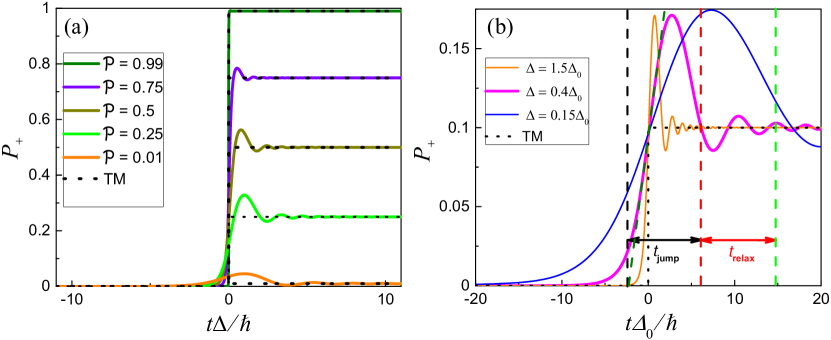
Figure 3: Single-passage Landau-Zener-Stückelberg-Majorana (LZSM) transition with different probabilities (a) and with different transition times for a fixed value of the transition probability $\mathcal{P}$ (b). In (a), we plot the time dependence of the upper-level occupation probability $P_{+}(t)$, hence demonstrating dynamics for a given value of the final LZSM probability $\mathcal{P}$. Black dashed curves are given by the transfer matrix (TM) method, while the solid colored curves show the numerical solution of the Schrödinger equation. In (b), all the curves are for a fixed LZSM probability $\mathcal{P}=0.1$, while both $\Delta$ and $v$ are varied; this demonstrates the impact of these parameters on the transient dynamics. Here, it is convenient to normalize time with a fixed value $\Delta_{0}$, to which also the $\Delta$ in the legend are related. The evolution is characterized by the two transition times: the jump time $t_{\mathrm{jump}}$ and the relaxation time $t_{\mathrm{relax}}$, which are shown in the figure for the thick magenta curve.

The second approach involves solving the Schrödinger equation with a linear excitation in terms of the parabolic cylinder functions $D_{\nu}(x)$ (see Appendix A.2). This approach gives a simple expression for the probability in the diabatic basis $\left\{\left|0\right\rangle,\left|1\right\rangle\right\}$. When solving the Schrödinger equation following Zener, it is natural to first introduce the dimensionless time, $\tau$, and then the related complex value, $z$, which can be called the “Zener” variable:

$$\tau=t\sqrt{\frac{v}{2\hbar}},\quad z=\tau e^{i\pi/4}\sqrt{2}e^{i\pi/4}=t\sqrt{\frac{v}{\hbar}}.$$ (16)

Then, starting the evolution from the ground level, $\left|E_{-}\right\rangle$ to the left in Fig. 2(a), we can obtain the time-dependent solution for the upper level occupation probability in diabatic basis (see Appendix A.2)

$$P_{\text{d}}(z)=\delta\exp\left(-\pi\delta/2\right)\left|D_{-1-i\delta}(-z)\right|^{2}.$$ (17)

To obtain transition dynamics for the upper level occupation probability in the adiabatic basis $\left\{\left|E_{-}(t)\right\rangle,\left|E_{+}(t)\right\rangle\right\}$, we use formulas Eqs. (5,6),

$$P_{\text{a}}(z)=\exp{\left(-\pi\delta/2\right)}\left|D_{-i\delta}(-z)\gamma_{+}-\sqrt{\delta}e^{-\frac{i\pi}{4}}D_{-1-i\delta}(-z)\gamma_{-}\right|^{2}.$$ (18)

An analytical solution like this has the advantage that one does not need to find all the values of the wave function from the initial time to the desired moment of time; this is in contrast to the numerical solution, where we need to calculate all the previous values of the wave function between the current and initial times.

In Fig. 3, we illustrate the evolution of the upper-level occupation probability, emphasizing several different aspects. In Fig. 3(a), we first fix several values of the final LZSM transition probability $\mathcal{P}$. These are defined by the adiabaticity parameter $\delta$, Eq. (8). Inverting the relation for $\mathcal{P}$, Eq. (7), we obtain the expression

$$\frac{\hbar v}{\Delta^{2}}=-\frac{\pi}{2\ln{(\mathcal{P})}},$$ (19)

which defines the ratio between $v$ and $\Delta$ for a given value of $\mathcal{P}$. With the defined values of $v$ and $\Delta$, we plot in Fig. 3(a) both the analytical solution (dashed lines), which is the step function from $0$ to $\mathcal{P}$, and the numerical solution (shown with the solid lines). We emphasize that, for the numerical approach, we can equally use either the direct solution for the Schrödinger equation or the formulas above, that is, Eqs. (17, 18). Note that with an increasing $\mathcal{P}$, the evolution becomes more similar to the analytical solution: the step function. Importantly, Fig. 3(a) vividly shows that the LZSM formula is robust and is valid in the whole range of TLS parameters, which was theoretically grounded in Refs. Hagedorn (1991); Joe (1994); Vitanov and Suominen (1999); Nakamura (2019).

In Fig. 3(b), we take the fixed value of the LZSM transition probability, $\mathcal{P}=0.1$. Then, for different curves, we simultaneously vary both $\Delta$ and $v$ to keep this $\mathcal{P}$ constant; the values of $\Delta$ are displayed. Figure 3(b) demonstrates that for a given $\mathcal{P}$, the other parameters drastically influence the dynamics. We characterize this using two transition times: $t_{\mathrm{jump}}$ and $t_{\mathrm{relax}}$. Consider now the definition and calculation of these important values; the details are presented in Appendix A.5. Importantly, the time scales of the transition processes are very different in the adiabatic and diabatic bases; thus, we describe the duration of the LZSM transition in both bases, following Vitanov (1999).

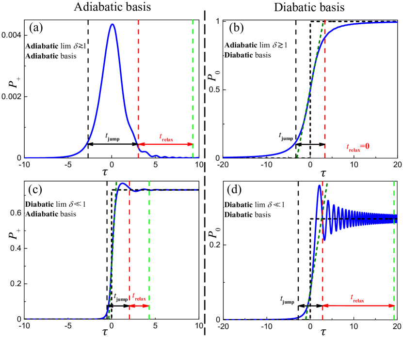
Figure 4: Dynamics of a single LZSM transition in the adiabatic basis (a,c) and in the diabatic basis (b,d). We illustrate two limit cases of the adiabaticity parameter: $\delta=2\gtrsim 1$ in $P_{+}(\tau)$ (a,b) and $\delta=0.05\ll 1$ in $P_{0}(\tau)$ (c,d). Horizontal black double arrows show $t_{\text{jump}}$ and red double arrows $t_{\text{relax}}$. Inclined dashed green lines show the derivative at the avoided crossing point, $\tau=0$. Recall that the dimensionless time is $\tau=t\sqrt{\frac{v}{2\hbar}}$.

Therefore, the transition process has two subsequent phases. The first one is when the probability jumps from the initial value $P(-\infty)$ to the vicinity of the final value $P(\infty)$. For the adiabatic basis, we have $P(\infty)=\mathcal{P}$, while for the diabatic basis, we have $P(\infty)=1-\mathcal{P}$. To quantify this time span $t_{\text{jump}}$, we note that the slope at zero is approximated by $P^{\prime}(0)\sim\Delta P/\Delta t$; replacing $\Delta P$ with $P(\infty)$ and $\Delta t$ with $t_{\text{jump}}$, we come to the definition

$$t_{\text{jump}}=\frac{P(\infty)}{P^{\prime}(0)}.$$ (20)

However, this definition is not always appropriate, as we discuss in Appendix A.5.

The second phase of evolution is the time when the probability exhibits damping oscillations around its final value $P(\infty)$; the duration of this process is denoted as $t_{\text{relax}}$. This relaxation time can be quantified by introducing the small parameter $\eta\ll 1$, which describes that, after $t_{\text{relax}}$, the amplitude of the oscillations becomes less than $\eta P(\infty)$.

We must distinguish the upper-level occupation probability in the adiabatic basis $P_{+}$ from the one in the diabatic basis $P_{0}$. The dynamics of the probabilities in different bases was theoretically investigated in Wubs et al. (2005); Danga et al. (2016) and experimentally in Zenesini et al. (2009); Tayebirad et al. (2010). We demonstrate the dynamics in these two bases in Fig. 4. For the adiabaticity parameter $\delta$, which describes the dynamics, we take two opposite limits: $\delta\ll 1$ (diabatic limit) and $\delta\gg 1$ (adiabatic limit). To be more precise, in the adiabatic limit, we take $\delta\gtrsim 1$ because with $\delta\gg 1$, the LZSM probability $\mathcal{P}=\exp{(-2\pi\delta)}$ becomes too small. With these four possibilities, in Fig. 4(a-d), we can observe quantitatively different types of dynamics.

Note that the relaxation times are also very different in the adiabatic and diabatic bases. Namely, the total transition time $\left(t_{\mathrm{LZSM}}=t_{\mathrm{jump}}+t_{\mathrm{relax}}\right)$ in the adiabatic limit ($\delta\gtrsim 1$) is much longer in the adiabatic basis than in the diabatic one. The opposite is true, as well, where the transition time in the diabatic limit ($\delta\ll 1$) is much longer in the diabatic limit than in the adiabatic one. In particular, for $\delta\gtrsim 1$, in the diabatic basis, there are no oscillations, which means there is zero relaxation time, $t_{\mathrm{relax}}^{\mathrm{d}}=0$.

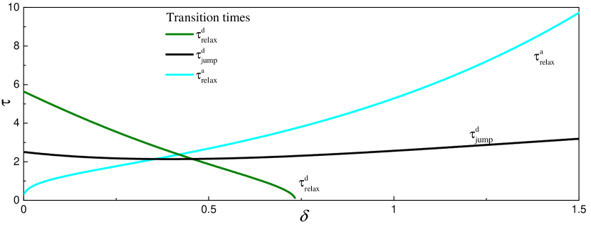
Figure 5: Transition times versus the adiabaticity parameter $\delta$. We plot both $\tau_{\text{relax}}^{\text{d}}$ and $\tau_{\text{jump}}^{\text{d}}$ for the transition in the diabatic basis and the relaxation time $\tau_{\text{relax}}^{\text{a}}$ in the adiabatic basis. We do not plot the jump time in the adiabatic basis because this is very close to the relaxation time, $\tau_{\text{jump}}^{\text{a}}\approx\tau_{\text{relax}}^{\text{a}}$. Here, the dimensionless time is $\tau=t(v/2\hbar)^{1/2}$. See Appendix A.5 for more details.

The jump and relaxation times can be obtained analytically from the exact solution that describes a single LZSM transition with linear excitation; the details are presented in Appendix A.5. Here, we define the simplified transition times $t_{\mathrm{LZSM}}$, which allow us to check the validity of the TM method. The characteristic time for a single-passage process is the sweeping time from the initial to the final state; if the driving is periodic, then the sweeping time equals half the period, $T_{\mathrm{d}}/2$. Hence, this characteristic time should be much larger than the LZSM transition time, which can be compactly written as follows (see Appendix A.5):

$$t_{\mathrm{LZSM}}^{\text{d}}\sim 4\sqrt{\frac{\hbar}{v}}\max\left\{1,\sqrt{\delta}\right\},$$ (21a)

$$t_{\mathrm{LZSM}}^{\text{a}}\sim\pi\sqrt{\frac{\hbar}{v}}\max\left\{\left(\frac{\delta}{\eta}\right)^{1/3},\left(\frac{\delta}{\eta}\mathcal{P}\right)^{1/6}\right\},$$ (21b)

in the diabatic and adiabatic bases, respectively. In Eq.(21b), $\eta\ll 1$ is the small parameter that describes the magnitude of the vicinity near the initial and final probabilities. These formulas are illustrated in Fig. 5, using $\tau=t(v/2\hbar)^{1/2}$.

II.3.3 Problems with nonlinearities

In general, the bias $\varepsilon(t)$ is not a linear function of time. To obtain the linear model, Eq. (2), which we considered before, we need to linearize the otherwise nonlinear bias around the point $t_{0}$, where $\varepsilon(t_{0})=0$:

$$\varepsilon(t)=\left(t-t_{0}\right)\left.\left(\frac{d\varepsilon}{dt}\right)\right|_{t=t_{0}}+o\left(t-t_{0}\right).$$ (22)

The linearization is appropriate if both the first derivative is nonzero and other terms are negligible. Then, the probability of the nonadiabatic transition is given by Eq. (7), with

$$\delta=\frac{\Delta^{2}}{4\hbar\left.\left(\frac{d\varepsilon}{dt}\right)\right|_{t=t_{0}}}.$$ (23)

Alternatively, instead of $\varepsilon(t)$, we can write the distance between the diabatic states: $\varepsilon(t)\rightarrow(E_{0}-E_{1})$. Even more generally, instead of $\Delta/2$, we can write the off-diagonal part of the Hamiltonian as the corresponding matrix element $V_{10}$; then, the adiabaticity parameter is written, as, for example, in Ref. Bendersky et al. (2013),

$$\delta=\left|\frac{V_{10}^{2}}{\hbar\left.\frac{d}{dt}\left(E_{0}-E_{1}\right)\right|_{t=t_{0}}}\right|.$$ (24)

Let us now consider the cases where the bias cannot be linearized or nonlinear corrections are relevant. Different nonlinear-level-crossing models were analyzed in Refs. Suominen et al. (1991); Vitanov and Suominen (1999); Ashhab et al. (2022). In that study, the authors used the Dykhne–Davis–Pechukas formula [this appears in the Appendix A.1 as Eq. (121)] to calculate the nonadiabatic transition probability when driven by different nonlinear biases $\varepsilon(t)$.

The biases can be grouped in two types: perturbative and essential nonlinearities. The former relates to the case when the linear term in Eq. (22) is dominant and the nonlinear corrections result in perturbative changes of the LZSM formula, while the latter relates to the case where there is no linear term and the essentially nonlinear bias is analyzed for the cases $\varepsilon(t)\propto t^{N}$ with $N=2,3,...~{}$Shimshoni and Gefen (1991); Vitanov and Suominen (1999); Lehto and Suominen (2012, 2015); Kaprálová-Žďánská (2022).

A special case of nonlinear LZSM tunneling relates to a TLS where the energy levels depend on the occupation of these levels. This may arise in a mean-field treatment of many-body systems where the particles predominantly occupy two energy levels Liu et al. (2002). Then, the system is described by the Hamiltonian

$$H_{C}(t)=-\frac{\Delta}{2}\sigma_{x}-\frac{\varepsilon(t)}{2}\sigma_{z}-\frac{C}{2}\left(P_{+}-P_{-}\right)\sigma_{z},$$ (25)

where $C$ is the parameter of nonlinearity, which describes the dependence of the energy levels on the state populations $P_{\pm}$. This parameter is not necessarily small and can be tunable. This form of the Hamiltonian is characteristic for the systems described by the Gross–Pitaevskii equation Ishkhanyan et al. (2010); Liu et al. (2016). This Hamiltonian —both with the linear driving, $\varepsilon(t)\propto t$, and periodic driving, $\varepsilon(t)\propto\sin\omega t$ —may be experimentally realized in several ways with BECs Zhang et al. (2008). If taking the nonlinearity into account for such systems, all the features of the nonadiabatic transitions should be revisited, including the quantum adiabatic theorem Wu and Niu (2003). When $\varepsilon(t)$ is a sinusoidal driving field, we should focus on nonlinear LZSM interferometry Li et al. (2018).

One more development of the linear LZSM problem can be obtained using an asymmetric linear bias, where the slopes are different on the left and right of the avoided-level crossing Damski and Zurek (2006). When the bias is a nonanalytic function, similar cases were studied in Ref. Garanin and Schilling (2002a). Various aspects of the nonlinearity of nonadiabatic transitions have been studied recently for realizations in such systems as a periodic lattice system Takahashi and Sugimoto (2018), spin qubit in a quantum wire Tchouobiap et al. (2018), superconducting qubits Wu et al. (2019), and topological systems Kam and Chen (2020).

Therefore, one can consider versatile nonlinear biases in the contexts of LZSM-like problems. At the end of this subsection, we illustrate this also with the idea of reverse engineering Kang et al. (2022). This is formulated as finding a Hamiltonian $\widetilde{H}(t)$ generating a given dynamics, here evolving in states that are the instantaneous eigenstates of a given Hamiltonian $H(t)$ Berry (2009). One formulation of this is the inverse LZSM problem, which is formulated as finding the bias $\varepsilon(t)$ resulting in any required time dependence of the level populations. This problem was formulated and solved in Ref. Garanin and Schilling (2002b). Then, in Ref. Shevchenko et al. (2012a), a similar problem was studied for a qubit-resonator system as restoring a driven qubit Hamiltonian, provided its stationary behavior is known; see also Barnes (2013). Another problem related to the reverse engineering approach is transitionless quantum driving, which is analogous to the explanation of reflectionless potentials. This was studied both theoretically Berry (2009); Villazon et al. (2021) and experimentally Bason et al. (2012); Xu et al. (2018). We address this in more detail in Sec. V.3, where we demonstrate that a Hamiltonian with appropriate nonlinear driving results in a transitionlesness system dynamics.

II.4 Some experimental observations

Driven TLSs are ubiquitous, which is true for the observations of the LZSM transition. In this section, we present illustrative examples of observations of the single passage LZSM transition.

• Historically, the first works by Landau, Zener, and Stückelberg related to inelastic atomic and molecular collisions. These described energy and charge exchange, as well as predissociation and associative recombination. The patterns observed in the scattering form the subject of collision spectroscopy. This was demonstrated for the inelastic scattering of He⁺ by Ne Coffey et al. (1969). In that work of more than half-century ago, the authors demonstrated both LZSM transitions and Stückelberg oscillations.

• As one realization of Majorana’s problem, a spin moves through the point of a vanishing magnetic field, also considered experimentally in Ref. Betthausen et al. (2012). In this case, a spin moved in a spin transistor over a distance of 50 micrometers while experiencing an adiabatically variable magnetic field. Alternation of adiabatic evolution and nonadiabatic transitions allows for accurate transistor control, making the spin transistor tolerant against disorder.

• Nonadiabatic transitions were experimentally shown in a strong electric field between the Stark states of highly excited (Rydberg) states in lithium Rubbmark et al. (1981). In contrast to molecular collisions, all the parameters there can be controlled accurately, which allowed obtaining quantitative agreement with theory in the two-level approximation, regarding their multilevel energy diagram. This allowed to better understand the dynamics of Rydberg atoms in rapidly rising electric fields.

• The tunneling dynamics of a BEC of ultracold atoms in a tilted periodic potential is realized by accelerating the lattice Zenesini et al. (2009); Tayebirad et al. (2010). Researchers studied LZSM tunneling both in the diabatic and adiabatic bases. Another study of an ultracold Fermi gas in a tunable honeycomb lattice was presented in Ref. Uehlinger et al. (2013). The authors realized two successive LZSM transitions without interference after sequentially passing through two Dirac points. The authors of Ref. Thalhammer et al. (2006) experimentally demonstrated the association and dissociation of the so-called Feshbach molecules, which are the molecules of a BEC formed by means of a Feshbach resonance.

• In quantum systems, it is often the case that many levels are relevant, and this will be a subject of one of the following sections. However, sometimes, only the dynamics of two close levels is relevant. We find this in the experiment of Zhao et al. (2017) on a large-spin system, $S=7/2$. The authors observed the nonadiabatic dynamics around one of the avoided-level crossings controlled with an external magnetic field in a Gd³⁺ impurity ion ensemble, which makes a qubit system with “a virtually unlimited relaxation time”.

• Qubit states in the NV center in diamond also have the advantage of good isolation. A single NV center electronic spin was coupled with a single nitrogen nuclear spin, creating a hybridized electronic-nuclear state Fuchs et al. (2011). In this case, the LZSM transition can transfer the excitation between the two subsystems, which was proposed as a basis for a room temperature quantum memory. To create the avoided-level crossing with the NV centers, the authors of Ref. Xu et al. (2019b) first applied a resonant microwave and considered the RWA, and then they explored the adiabatic evolution and nonadiabatic transitions.

• Micrometer-size superconducting qubits allow the realization of macroscopically distinct quantum states. The nonadiabatic transitions between them were demonstrated for a variety of JJ-based qubits, including the flux Izmalkov et al. (2004), quantronium Ithier et al. (2005), charge (Cooper pair sluice) Gasparinetti et al. (2012), and phase Tan et al. (2015) qubits. In these works, it was demonstrated that such measurements are useful for probing and controlling both the qubits themselves and the coupled microscopic systems, hence providing a fast and sensitive tool to study and control qubits.

• Another mesoscopic-size platform is provided by (double-)quantum dots. LZSM transitions were studied in singlet-triplet qubits in silicon in Harvey-Collard et al. (2019); Khomitsky and Studenikin (2022). In this case, tunneling was demonstrated to be useful to extract the spin-orbit coupling. Besides the electronic degrees of freedom, quantum dots can be used to manipulate the nuclear spin ensemble with chirped magnetic resonance pulses Munsch et al. (2014).

• Somewhat unexpectedly, LZSM physics is related to second-order phase transitions, of which the dynamics is described by the KZM. We discuss this in the section III.1.2, but here, to better describe the second-order phase transitions dynamics, we present a variety of systems in which the KZM was experimentally studied in laboratories. The KZM correctly predicts the creation of topological defects during a single passage through a symmetry-breaking transition. Following the original proposal by Zurek (1985), defects (vortices) in superfluid ⁴He were created during the phase transition induced by fast expansion through the critical density, crossing the $\lambda$–line on the pressure–temperature phase diagram Hendry et al. (1994). The vortices in superfluid ³He were created using neutron-induced nuclear reaction ($n+$ ³He$\rightarrow$ ³H$+p$) to heat small regions of superfluid ³He above the superfluid transition temperature Bäuerle et al. (1996); Ruutu et al. (1996). The probability to trap a single flux line in annular JJs was shown to work because of a causal KZM rather than because of thermal activation Monaco et al. (2009). Other examples include zig-zag defects in buckled chains of ions (introduced above, in Fig. 1), defect textures in liquid crystals, flux lines in superconductors quenched through the critical temperature, and spin domains in Bose condensates realized in a shaken optical lattice. For a review, see Pyka et al. (2013); Hedvall and Larson (2017); Dziarmaga (2010).

• The analogy between nonadiabatic transitions in classical and quantum mechanics has been known for quite a long time Maris and Xiong (1988). However, this idea was realized only recently on mechanical resonators Faust et al. (2012), in which the authors demonstrated that the energy transfer between the two modes of a nanomechanical resonator obeys LZSM behavior. We explore analogies and studies in a separate section VI.

For a description of additional experimental observations, see Sec. IV. We would like to note that in many cases it is possible to observe either single-passage LZSM transitions or multiple-passage LZSM interference, which are described here and in Sec. IV, respectively. For this reason, we describe the related experiments in these two places. Before moving to the latter observations, let us consider the underlying physics first.

II.5 Transfer matrix (TM) method

Consider now the dynamics during a single-passage transition as a sequence of three stages:

• (i) adiabatic evolution starting from the time $t_{\mathrm{i}}<0$ until an avoided-level crossing is reached,

• (ii) a nonadiabatic transition very near $t=0$, and

• (iii) adiabatic evolution starting from an avoided-level crossing passed until the time $t_{\mathrm{f}}=-t_{\mathrm{i}}>0$.

The wave function can be expanded in the basis of the adiabatic eigenstates $\left|E_{\pm}(t)\right\rangle$:

$$\left|\psi(t)\right\rangle=\alpha(t)\left|E_{-}(t)\right\rangle+\beta(t)\left|E_{+}(t)\right\rangle=\binom{\alpha(t)}{\beta(t)}.$$ (26)

The normalization condition results in all the transfer matrices being unitary ones. Consider this for both (i,iii) adiabatic and (ii) nonadiabatic evolutions. For the former, from a nonstationary Schrödinger equation, Eq. (15), we obtain the adiabatic time-evolution operator

$$\color[rgb]{1,.5,0}\boxed{\color[rgb]{0,0,0}U(\zeta(t,t_{\mathrm{i}}))=\begin{pmatrix}\exp{\left[-i\zeta(t,t_{\mathrm{i}})\right]}&\ 0\\ 0&\exp{\left[i\zeta(t,t_{\mathrm{i}})\right]}\end{pmatrix}=\exp{\left[-i\zeta(t,t_{\text{i}})\sigma_{z}\right]},\color[rgb]{1,.5,0}}\color[rgb]{0,0,0}$$ (27)

where $\zeta(t,t_{\mathrm{i}})$ is the phase accumulated during the adiabatic evolution from the time $t_{\text{i}}$ until the time moment $t$

$$\zeta(t,t_{\mathrm{i}})=\frac{1}{2\hbar}\int_{t_{\mathrm{i}}}^{t}\Delta E(t)\text{ }dt.$$ (28)

Hence, the adiabatic evolution is described by the relation

$$\left|\psi(t)\right\rangle=U(\zeta(t,t_{\mathrm{i}}))\left|\psi(t_{\mathrm{i}})\right\rangle,$$ (29)

which corresponds to no transitions between the adiabatic states, with only the phase difference accumulated.

Next, consider an impulse-type transition at $t=0$. In Appendix A, we obtain the transition matrix in the diabatic basis; after transferring from the diabatic basis to the adiabatic one, using Eq. (6) and assuming $\varepsilon(t)\gg\Delta$, we obtain the transition matrix

$$\color[rgb]{1,.5,0}\boxed{\color[rgb]{0,0,0}N=\begin{pmatrix}Re^{-i\phi_{\text{S}}}&-T\\ T&Re^{i\phi_{\text{S}}}\end{pmatrix},\color[rgb]{1,.5,0}}\color[rgb]{0,0,0}$$ (30)

where

$$T=\sqrt{\mathcal{P}}=\text{ Transition coefficient,}$$ (31a)

$$R=\sqrt{1-\mathcal{P}}=\text{ Reflection coefficient;}$$ (31b)

$\phi_{\text{S}}$ is the Stokes phase (9), which appears in the theory of second-order differential equations. For more details, see Nikitin and Reznikov (1972); Child (1996); Kayanuma (1997); Gasparinetti et al. (2011), particularly for how this phase appears in terms of the Bloch vector evolution and Berry phase accumulation. Hence, the impulse-type nonadiabatic transition at around $t=0$ is described by

$$\left|\psi(+0)\right\rangle=N\text{ }\left|\psi(-0)\right\rangle.$$ (32)

Note that given the asymptotics of the gamma function, the monotonous function ${\phi}_{\text{S}}(\delta)$ changes from $0$ in the adiabatic limit ($\delta\gg 1$) to $\pi/4$ in the diabatic limit ($\delta\ll 1$).

Now, we can define the total single-transition evolution matrix in the general case $\zeta_{\text{i}}\equiv\zeta(0,t_{\text{i}})\neq\zeta(t_{\text{f}},0)\equiv\zeta_{\text{f}}$

$$U(\zeta_{\text{f}})NU(\zeta_{\text{i}})=\begin{pmatrix}R\exp{[-i(\phi_{\text{S}}+\zeta_{\text{i}}+\zeta_{\text{f}})]}&-T\exp{[-i(\zeta_{\text{i}}-\zeta_{\text{f}})]}\\ T\exp{[i(\zeta_{\text{i}}-\zeta_{\text{f}})]}&R\exp{[i(\phi_{\text{S}}+\zeta_{\text{i}}+\zeta_{\text{f}})]}\end{pmatrix}.$$ (33)

We also can find the total single-transition evolution matrix in the case of symmetric adiabatic evolution $\zeta(0,t_{\text{i}})=\zeta(t_{\text{f}},0)\equiv\zeta$,

$$U(\zeta)NU(\zeta)=\begin{pmatrix}R\exp{[-i(\phi_{\text{S}}+2\zeta)]}&-T\\ T&R\exp{[i(\phi_{\text{S}}+2\zeta)]}\end{pmatrix}.$$ (34)

Note that when we consider the inverse transition we should replace the direct-transition matrix $N$ with the inverse transition matrix

$$N_{\text{inverse}}\equiv N^{\top},$$ (35)

which is the transposed matrix, see Eq. (146a), and Ref. Teranishi and Nakamura (1998).

As a generic initial condition at $t=t_{\mathrm{i}}$, we take a superposition state

$$\left|\psi(t_{\mathrm{i}})\right\rangle=\alpha(t_{\mathrm{i}})\left|E_{\_}(t_{\mathrm{i}})\right\rangle+\beta(t_{\mathrm{i}})\left|E_{+}(t_{\mathrm{i}})\right\rangle,$$ (36)

where $\left|E_{\pm}(t)\right\rangle$ are the instantaneous eigenstates of the time-dependent Hamiltonian $H(t)$ and

$$\begin{cases}\alpha(t_{\mathrm{i}})=\sqrt{P_{-}(t_{\mathrm{i}})},\\ \beta(t_{\mathrm{i}})=\sqrt{P_{+}(t_{\mathrm{i}})}e^{i\phi_{\text{i}}},\end{cases}$$ (37)

where $P_{\pm}(t_{\mathrm{i}})$ are the occupation probabilities of the respective states and $\phi_{\mathrm{i}}$ describes the initial phase difference. Importantly, for a superposition state, the phase difference significantly influences the dynamics Emmanouilidou et al. (2000); Wubs et al. (2005). Now, with the evolution matrix $UNU$, we can obtain the final upper-level occupation probability

$$P_{+}(t_{\mathrm{f}})=T^{2}P_{-}(t_{\mathrm{i}})+R^{2}P_{+}(t_{\mathrm{i}})-2RT\sqrt{P_{-}(t_{\mathrm{i}})P_{+}(t_{\mathrm{i}})}\cos(-{\phi}_{\text{S}}-2\zeta+\phi_{\text{i}}).$$ (38)

This formula describes several important aspects. First, when the cosine equals $+1$ or $-1$, we have maximal and minimal excitation probabilities $P_{+}^{\max/\min}(t_{\mathrm{f}})$, respectively. These correspond to the constructive and destructive interference of the incoming states. The respective conditions are

$$\begin{cases}-{\phi}_{\text{S}}-2\zeta+\phi_{\text{i}}=2\pi n\>\>\>\>\>\>\>\>\>\>\>\>\>\>\>\text{ for }P_{+}^{\max},\\ -{\phi}_{\text{S}}-2\zeta+\phi_{\text{i}}=2\pi(n+\frac{1}{2})\>\>\>\text{ for }P_{+}^{\min},\end{cases}$$ (39)

where $n$ is an integer.

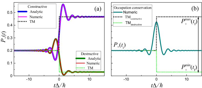
Figure 6: Nonadiabatic transition with a superposition state. Comparison of the numerical, analytical, and transfer matrix (TM) solutions for a single LZSM transition starting from a superposition state. For this, we took $\alpha(t_{\text{i}})=\sqrt{0.2}$ and $\beta(t_{\text{i}})=\sqrt{0.8}e^{i\phi_{\text{i}}}$, here with two cases for the phase difference: one for a destructive interference case, $\phi_{\text{i}}\ =5\pi/3$, and another case for constructive interference, $\phi_{\text{i}}\ =2\pi/3$ in (a), which can realize the maximum and minimum possible values of the final probability, Eqs. (38, 39), and the probability-conserving case in (b), here with the initial phase difference defined in Eq. (41) and a transition without changes in the probability. The black double-arrow shows the range of the possible final values of the probability. This demonstrates the dramatic dependence of the evolution on the initial phase difference and the role of interference.

Second, note that the range between the extremal values $P_{+}^{\min}$ and $P_{+}^{\max}$ includes the initial probability $P_{+}(t_{\mathrm{i}})$. This means that we can select the value of the initial phase difference $\phi_{\text{i}}$, which gives us the transition without any change of the probability so that

$$P_{+}(t_{\mathrm{f}})=P_{+}(t_{\mathrm{i}}).$$ (40)

This process can be named occupation-conserving transition (OCT). This takes place for the phase difference $\phi_{\text{i}}=\phi_{\text{i}}^{\mathrm{OCT}}$

$$\phi_{\text{i}}^{\mathrm{OCT}}=-{\phi}_{\text{S}}-2\zeta+\arccos\left[\frac{T\left(P_{+}(t_{\mathrm{i}})-1/2\right)}{R\sqrt{P_{+}(t_{\mathrm{i}})P_{-}(t_{\mathrm{i}})})}\right].$$ (41)

Note that this is possible only for a superposition initial state; when starting from a ground state, there is no effect on the phase difference.

In the case of starting from a superposition initial state, all these dynamical features are illustrated in Fig. 6. In this figure, we compare the numerical solution with the analytical one, which is given by Eq. (132a), with a perfect agreement between the two. In addition, we show the asymptotic solution described by the transfer matrix method with a step-like transition, as described by the equations above. For the calculations, we take the adiabaticity parameter $\delta=0.4$, which corresponds to the LZSM probability $\mathcal{P}=0.08$. In Fig. 6, we present the solutions for three different cases: for constructive interference with initial phase difference $\phi_{\text{i}}\ =\phi_{1}=2\pi/3$, for destructive interference with $\phi_{\text{i}}\ =\phi_{2}=5\pi/3$, and for the probability-conserving case with $\phi_{\text{i}}=\phi_{\text{i}}^{\mathrm{OCT}}$, Eq. (41). Note that $\mathcal{P}$ is the probability of excitation if starting from the ground state, while now, we can demonstrate a more general case of starting from the superposition state. This demonstrates that the upper-level occupation probability $P_{+}(\infty)$ is essentially different from $\mathcal{P}$ and that this is defined by not only $\delta$, but also by the initial condition.

III Repetitive passage: interference

In the previous section, we considered a TLS when driven by a linear drive $\varepsilon(t)=vt$. From now on, we consider the evolution for a generic periodic bias with an offset $\varepsilon_{0}$,

$$\color[rgb]{1,0,0}\boxed{\color[rgb]{0,0,0}\varepsilon(t)=\varepsilon_{0}-A\cos\omega t.\color[rgb]{1,0,0}}\color[rgb]{0,0,0}$$ (42)

We now consider several approaches.

III.1 Adiabatic-impulse model (AIM)

III.1.1 Double-passage and multiple-passage cases

The adiabatic-impulse model is possibly the most intuitive model for describing the repetitive LZSM passage Damski and Zurek (2006); Tomka et al. (2018). In this model, we consider the evolution of the TLS beyond the avoided-crossing region as adiabatic evolution, and in the avoided-crossing region, we consider the diabatic evolution of the TLS. Also, we approximate the avoided-crossing region by the point of minimum distance between energy levels. Therefore, we have the adiabatic evolution everywhere save for the points of the minimal distance between energy levels, where nonadiabatic LZSM transitions occur. Thus, the AIM consists in that the evolution is modeled (approximated) as adiabatic one besides the non-adiabatic transitions in the avoided-level-crossing points (where the driving is approximated as a linear one); given these approximations, instead of AIM this technique can alternatively be called adiabatic-impulse approximation. Essentially, the AIM is described by using the TM method. The latter was developed by Bychkov and Dykhne (1970); Averbukh and Perel’man (1985); Kayanuma (1993); Vitanov and Garraway (1996); Garraway and Vitanov (1997); Teranishi and Nakamura (1998); Delone and Krainov (2012).

In the section “Transfer Matrix Method”  we introduced the matrices $U$ and $N$ for the adiabatic evolution and nonadiabatic impulse-type transition, respectively. This describes the evolution during half the period. When speaking about driven systems, it is illustrative to sequentially consider three cases: single-passage transition probability, double-passage case, and the multiple-passage transition probabilities Nikitin (2006). We now consider the evolution during one full period and then during many periods, to which we refer to as double-passage and multiple-passage cases, respectively.

The adiabatic energy levels

$$E_{\pm}(t)=\pm\frac{\Delta E(t)}{2}=\pm\frac{1}{2}\sqrt{\Delta^{2}+\varepsilon(t)^{2}}$$ (43)

have a minimum distance (equal to $\Delta$) at times $t_{1,2}+nT_{\mathrm{d}}$, where $\omega t_{1}=\arccos(\varepsilon_{0}/A)$ and $\omega t_{2}=\pi+\omega t_{1}$, see Fig. 7(a).

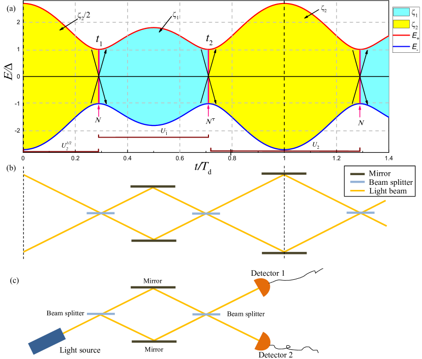
Figure 7: Evolution of energy levels in the adiabatic-impulse model (AIM). (a) The time-dependent adiabatic energy levels $E_{\pm}(t)$ define two stages of evolution: first, the adiabatic evolution with the transfer matrices $U_{1}$ and $U_{2}$ and, second, the transition in the region of avoided level crossing as determined by the matrix $N$. Here we consider a single-period evolution from $t=0$ to $t=T_{\text{d}}$, which is the time between the two vertical dashed black lines in panel (a). This evolution is described by $\sqrt{U_{2}}N_{\text{inverse}}U_{1}N\sqrt{U_{2}}$, in terms of time-evolution matrices, where $\sqrt{U_{2}}=U(\zeta_{2}/2)$. (b) Equivalent optical scheme based on Mach-Zehnder interferometer, where the optical beam splitters are analogous to the transition points in (a). The trajectories can have different lengths (e.g. due to the moving upper mirror) resulting in the relative phases of the two partial rays, in analogy with the wave-function phase difference accumulated during the LZSM transitions in (a). (c) Typical scheme of the optical Mach-Zehnder interferometer, analogous to the double-passage LZSM problem.

The adiabatic evolution is described by

$$U_{1,2}=\exp(-i\zeta_{1,2}\sigma_{z})$$ (44)

with the phase differences

$$\zeta_{1}=\frac{1}{2\hbar}\int\limits_{t_{1}}^{t_{2}}\Delta E(t)dt,\ \ \ \ \ \zeta_{2}=\frac{1}{2\hbar}\int\limits_{t_{2}}^{t_{1}+T_{\mathrm{d}}}\Delta E(t)dt.$$ (45)

The nonadiabatic transitions between the states $\left|E_{\pm}(t)\right\rangle$ are described by the transfer matrix $N$, which is true for both transitions and corresponds to the sweeping occurring both to the right and left in Fig. 2, respectively. Note that the evolution in the diabatic basis should be described differently Ashhab et al. (2007); Shevchenko et al. (2010). In some papers Shevchenko et al. (2010) double passage evolution is described starting at the quasicrossing point and finishing also at the quasicrossing point, see Vitanov and Garraway (1996); Cucchietti et al. (2007). And that way gives a correct result for averaged level occupations under the periodic driving $\Xi=N_{\text{inverse}}U_{2}NU_{1}=\left(\begin{array}[]{cc}\Xi_{11}&\Xi_{12}\\ -\Xi_{12}^{\ast}&\Xi_{11}^{\ast}\end{array}\right)$.

It is more convenient to describe the evolution starting far from the quasicrossing point and finishing also far from it. Then the double-passage evolution takes place after the full period and is described by the double-passage transfer matrix

$$\color[rgb]{1,.5,0}\boxed{\color[rgb]{0,0,0}\Xi\equiv\sqrt{U_{2}}N_{\text{inverse}}U_{1}N\sqrt{U_{2}}=\left(\begin{array}[]{cc}\Xi_{11}&\Xi_{12}\\ \Xi_{12}&\Xi_{11}^{\ast}\end{array}\right),\color[rgb]{1,.5,0}}\color[rgb]{0,0,0}$$ (48)

where

$$\Xi_{11} = -R^{2}e^{-i\zeta_{+}}-T^{2}e^{-i\zeta_{-}}$$ (49a)

$$\Xi_{12} = -2iRT\sin(\Phi_{\mathrm{St}})=-\Xi_{12}^{\ast},$$ (49b)

$$\zeta_{+} = \zeta_{1}+\zeta_{2}+2\phi_{\mathrm{S}},\text{ \ }\zeta_{-}=\zeta_{1}-\zeta_{2},\text{ \ }\Phi_{\mathrm{St}}=\phi_{\mathrm{S}}+\zeta_{1},$$ (49c)

for the inverse transition matrix $N_{\text{inverse}}$ see Eq. (35). We obtain the same $\Xi_{11}$ as in Ref. Shevchenko et al. (2010) for the double transition, but $\Xi_{12}$ is different due to using a shifted driving signal.

From Eq. (49b), one can see that the upper-level occupation probability, if starting from the ground state, becomes

$$\color[rgb]{0,1,0}\boxed{\color[rgb]{0,0,0}P_{+}^{\mathrm{double}}=\left|\Xi_{12}\right|^{2}=4\mathcal{P}(1-\mathcal{P})\sin^{2}\Phi_{\mathrm{St}}.\color[rgb]{0,1,0}}\color[rgb]{0,0,0}$$ (50)

In this way, following Zener’s approach we confirmed the Stückelberg formula, Eq. (11).

Here, an instructive analogy with the Mach–Zehnder interferometer is appropriate Oliver et al. (2005); Petta et al. (2010); Burkard (2010); Ma et al. (2011). We illustrate this analogy graphically: Fig. 7(b) shows that our dynamics in Fig. 7(a) is analogous to multiple periodic Mach-Zehnder interferometers Oliver et al. (2005), and Fig. 7(c) shows that our double-passage LZSM problem is analogous to an optical Mach-Zehnder interferometer Burkard (2010). Namely, passing the avoided-level crossing is analogous to light passing a partly transparent mirror functioning as a beam splitter with the coefficients $R$ and $T$. After the two beams meet, the outcome is the result of the interference, which depends on the phase difference $\Phi_{\mathrm{St}}$. For more about double-passage regime theory, see, e.g., Saxon and Olson (1975); Garraway and Stenholm (1992b); Garraway and Suominen (1995); Nagaya et al. (2007); Gasparinetti et al. (2011).

For the multiple-passage case, after $n$ full periods, the time evolution is described by the following evolution matrices:

$$U\left(t,t_{1}+nT_{\mathrm{d}}\right)\Xi^{n}\>\>\ \ \text{ for }\>\>t-nT_{\mathrm{d}}\in\left(t_{1},t_{2}\right),$$ (51)

$$U\left(t,t_{2}+nT_{\mathrm{d}}\right)NU_{1}\Xi^{n}\>\>\ \text{ for }\>\>t-nT_{\mathrm{d}}\in\left(t_{2},t_{1}+T_{\mathrm{d}}\right).$$ (52)

Hence, the system state after $n$ full periods of evolution is given by $\Xi^{n}$, which reads as Bychkov and Dykhne (1970)

$$\Xi^{n} = \left(\begin{array}[]{cc}\Xi_{n11}&\Xi_{n12}\\ -\Xi_{n12}^{\ast}&\Xi_{n11}^{\ast}\end{array}\right),$$ (53c)

$$\Xi_{n11} = \cos n\phi+i\text{Im}\Xi_{11}\frac{\sin n\phi}{\sin\phi},\text{ \ \ }\>\>\Xi_{n21}=\Xi_{21}\frac{\sin n\phi}{\sin\phi},\text{ \ }\phi=\arccos\text{Re}\Xi_{11}.\text{\ }$$ (53d)

Then, for the respective upper-level occupation probability, if starting from the ground state, we obtain
$$P_{+}(n)=\left|\Xi_{n12}\right|^{2}$$, which gives

$$\color[rgb]{0,1,0}\boxed{\color[rgb]{0,0,0}P_{+}(n)=\left|\Xi_{12}\right|^{2}\frac{\sin^{2}n\phi}{\sin^{2}\phi}=\underset{P_{+}^{\mathrm{double}}}{\underbrace{4\mathcal{P}(1-\mathcal{P})\sin^{2}\Phi_{\mathrm{St}}}}\frac{\sin^{2}n\phi}{\sin^{2}\phi}.\color[rgb]{0,1,0}}\color[rgb]{0,0,0}$$ (54)

This describes the time evolution, with $n$ denoting the integer number of periods passed, as shown in Fig. 8. Note the impressive agreement between the results of the AIM and numerics; see also Mukherjee et al. (2018); Kuno (2019). For a similar description of the multilevel systems, see Qin (2016); Neilinger et al. (2016); Niranjan et al. (2020); Suzuki and Nakazato (2022).

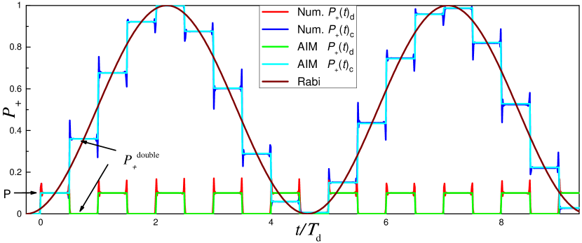
Figure 8: Constructive versus destructive interference. Comparison of the upper-level occupation probability obtained numerically and from the AIM in the regime of constructive interference (blue and light blue curves: $P_{+}(t)_{\mathrm{c}}$ calculated numerically and in the AIM, respectively) and destructive interference (red and green curves: $P_{+}(t)_{\mathrm{d}}$ calculated numerically and in the AIM, respectively). The light blue and green curves present the analytical solutions, while the blue and red curves show numerical solutions. We take the following parameters: $\varepsilon_{0}=0$ (then $\zeta_{1}=\zeta_{2}$) and $\mathcal{P}=0.1$; and the conditions for the constructive and destructive interference, $\zeta_{1}+{\phi}_{\mathrm{S}}=\pi k$ and $=\pi k+\frac{\pi}{2}$, respectively; these conditions define $\omega$ and $A$. The brown line is plotted with Rabi frequency obtained in Eq. (55).

Rabi oscillations from LZSM transitions

Adiabatic dynamics is characterized by small steps which, under resonance condition, result in Rabi-like oscillations Garraway and Stenholm (1992a); Pu et al. (2000); Shevchenko et al. (2005). This can be seen in Fig. 8. The frequency of these Rabi-like oscillations can be found from Eq. (54) if we identify $\sin^{2}(n\phi)$ with $\sin^{2}\left(\frac{\Omega_{\mathrm{R}}}{2}t\right)$ Ashhab et al. (2007); Neilinger et al. (2016); Liu et al. (2021). Then, we note that during one driving period, the integer $n$ changes by unity, and this corresponds to changing the time $t$ by $2\pi/\omega$. With this, we obtain the relation for the coarse-grained oscillations

$$\color[rgb]{1,.5,0}\boxed{\color[rgb]{0,0,0}\Omega_{\mathrm{R}}=\frac{\omega}{\pi}\left|\phi\right|=\frac{\omega}{\pi}\arccos\left[(1-\mathcal{P})\cos\zeta_{+}-\mathcal{P}\cos\zeta_{-}\right].\color[rgb]{1,.5,0}}\color[rgb]{0,0,0}$$ (55)

This formula correctly describes the Rabi oscillations induced by strong driving, as studied in Refs. Zhou et al. (2014); Neilinger et al. (2016). Indeed, we note that for a small offset $\varepsilon_{0}/A\ll 1$, the expressions for $\zeta_{\pm}$ can be simplified:

$$\zeta_{1}+\zeta_{2}\approx 2A/\hbar\omega\>\>\text{ \ and \ }\>\>\zeta_{1}-\zeta_{2}\approx\pi\varepsilon_{0}/\hbar\omega.$$ (56)

With this, in the adiabatic limit ($\mathcal{P}\ll 1$), we obtain $\Omega_{\mathrm{R}}\sim A/\hbar$. This correctly describes the resonant Rabi frequency and justifies the term “Rabi oscillations”, which we used above.

The long-time averaged occupation probability, is given by averaging over large $n$,

$$\color[rgb]{0,1,0}\boxed{\color[rgb]{0,0,0}\overline{P_{+}}=\frac{\left|\Xi_{21}\right|^{2}}{2\sin^{2}\phi}=\frac{1}{2}\frac{\left|\Xi_{21}\right|^{2}}{\left|\Xi_{21}\right|^{2}+(\text{Im}\Xi_{11})^{2}}.\color[rgb]{0,1,0}}\color[rgb]{0,0,0}$$ (57)

It follows that the upper-level occupation probability $\overline{P_{+}}$ is maximal at Im$\Xi_{11}=0$. This results in the resonance condition:

$$(1-\mathcal{P})\sin\zeta_{+}-\mathcal{P}\sin\zeta_{-}=0.$$ (58)

In particular, in the adiabatic (slow) and diabatic (fast) limits, the resonance condition takes the following forms:

$$\zeta_{1}+\zeta_{2} = k\pi\>\>\>\>\>\text{ for }\delta\gg 1\>\>\>\>\>\text{(adiabatic)},$$ (59a)

$$\zeta_{1}-\zeta_{2} = k\pi\>\>\>\>\>\text{ for }\delta\ll 1\>\>\>\>\>\text{(diabatic)}.$$ (59b)

Figure 9: LZSM interferograms calculated within the adiabatic-impulse model (AIM). (a) The low-frequency driving corresponding to the slow-passage regime, Eq. (60), with $\hbar\omega/\Delta=0.8<1$. (b) The high-frequency driving corresponds to the fast-passage limit, Eq. (62), with $\hbar\omega/\Delta=1.4>1$.

With the limiting expressions (53), the resonance condition for the adiabatic limit reads $2A\approx k\pi\hbar\omega$, and for the diabatic limit, this gives $\varepsilon_{0}\approx k\hbar\omega$. Because in the diabatic limit $\Delta$ is relatively small $(\Delta E\approx\left|\varepsilon_{0}\right|),$ the latter condition can be interpreted as an exchange of $k$ photons between the driving field and our two-level system.

In the slow passage limit, where $\delta\gg 1$ and $\mathcal{P}\ll 1$, we directly obtain the time-averaged occupation probability of the upper state:

$$\color[rgb]{0,1,0}\boxed{\color[rgb]{0,0,0}\overline{P_{+}}=\frac{\mathcal{P}(1+\cos\zeta_{+}\cos\zeta_{-})}{\sin^{2}\zeta_{+}+2\mathcal{P}(1+\cos\zeta_{+}\cos\zeta_{-})},\color[rgb]{0,1,0}}\color[rgb]{0,0,0}$$ (60)

which describes the dependence on the variable and controllable parameters $\varepsilon_{0}$, $A$, and $\omega$.

In the case of fast passage, where $\left(1-\mathcal{P}\right)\approx 2\pi\delta\ll 1$, there is a large probability ($\mathcal{P}\sim 1$) for transitions between the adiabatic states in a single passage, while the transition probability between diabatic states is small, $\left(1-\mathcal{P}\right)\ll 1$. Hence, we consider the time-averaged probability of the upper diabatic state $P_{\mathrm{up}}$. Then, one can obtain:

$$\overline{P}_{\mathrm{up}}=\frac{1}{2}\frac{4\pi\delta\cos^{2}(\zeta_{2}-\pi/4)}{\sin^{2}\zeta_{-}+4\pi\delta\cos^{2}(\zeta_{2}-\pi/4)}.$$ (61)

On resonance, we have $\zeta_{-}=k\pi$ and $\overline{P}_{\mathrm{up}}=1/2$. Then, in particular, for a small offset, with $\zeta_{-}\approx\pi\varepsilon_{0}/\hbar\omega$, we obtain the resonance frequency $\hbar\omega^{(k)}=\varepsilon_{0}/k$, meaning that the resonance transitions are described by their multi-photon relation. In the vicinity of the $k$-th resonance, for $\omega\sim\omega^{(k)}$, to first approximation in $\varepsilon_{0}/A$, we obtain

$$\color[rgb]{0,1,0}\boxed{\color[rgb]{0,0,0}\overline{P}_{\mathrm{up}}^{(k)}=\frac{1}{2}\frac{\Delta_{k}^{2}}{\Delta_{k}^{2}+\left(k\hbar\omega-\varepsilon_{0}\right)^{2}},\color[rgb]{0,1,0}}\color[rgb]{0,0,0}$$ (62)

$$\Delta_{k}=\Delta\sqrt{\frac{2\hbar\omega}{\pi A}}\cos{\left(\frac{A}{\hbar\omega}-\frac{\pi}{4}(2k+1)\right)}.$$

The total probability $\overline{P}_{\mathrm{up}}$ is obtained as the sum of the partial contributions $\overline{P}_{\mathrm{up}}^{(k)}$. Note that the above derivation within the AIM assumes that the excitation probability may become nonzero when the energy quasicrossing is reached, that is, at $\left|\varepsilon_{0}\right|<A$; otherwise, at $\left|\varepsilon_{0}\right|>A$, this model gives a zero transition probability.

Coherent destruction of tunneling (CDT)

From the formulas above, we can see that there are conditions under which the driven system can stay unexcited, with no tunneling between the states, even under the impact of a strong resonant drive. This phenomenon is known as coherent destruction of tunnelling or CDT Grossmann et al. (1991) and can be applied for controlling tunneling in TLSs Llorente and Plata (1992); Hu et al. (2022). It can be understood and described as either a degeneracy of the Floquet quasienergies Hijii and Miyashita (2010) or, equivalently, as a result of destructive LZSM interference Kayanuma (1994); Kayanuma and Saito (2008). Indeed, from Eq. (54), looking at a general case, there are no transitions between the states under the antiresonant condition, $\Xi_{21}=0$. Another case is Eq. (62), which gives zero excited-state populations if driven with the amplitude $A=A_{k}\equiv(\pi/4)(2k-1)\hbar\omega$.

Complete CDT is only possible for isolated systems, such as the ones we consider here; taking into account dissipation spoils the effect Miao and Zheng (2016a). CDT happens to be important for the description of various systems: transitions in graphene Gagnon et al. (2016, 2017) or in biomolecular protein—solvent reservoirs in photosynthetic light harvesting complexes Eckel et al. (2009); for a review of CDT in different systems, see Wubs (2010).

Latching modulation

Our derivations in this section are mainly developed for sinusoidal driving. These can be adapted to a description of any other periodic driving, $\varepsilon(t+T_{\mathrm{d}})=\varepsilon(t)$. Particularly, consider now the situation when a TLS is driven so that the level separation is switched abruptly between two values and is kept constant otherwise Silveri et al. (2015). In this case, we have the bias

$$\varepsilon(t)=\varepsilon_{0}+A\text{ sgn}\left[\cos(\omega t)\right],$$ (63)

which results in the periodic latching modulation of the qubit energy levels. Direct application of the LZSM approach would give infinite speed $v$, resulting in exact unit probability $\mathcal{P}=1$ with no interference. In this case, with $v=\infty$, the AIM is not directly applicable because then the width of the transition region becomes infinite: $vt^{\text{d}}_{\mathrm{LZSM}}\sim\sqrt{\hbar v}$, see Eq. (21a). This has been analyzed in Ref. Silveri et al. (2015), where the generalization of the AIM is presented. Interestingly, most of the formulas above, which describe the upper-level occupation probability, remain valid with only one important substitution: now, instead of the LZSM probability $\mathcal{P}$, we write the sudden-switch transition probability $p_{s}=\langle\psi_{+}^{(l)}|\psi_{-}^{(r)}\rangle$, which occurs between the lower state in one latch position $\left|\psi_{-}^{(r)}\right\rangle$ and the upper state in the other latch position $\left|\psi_{+}^{(l)}\right\rangle$. The successful application of the AIM with this substitution $\mathcal{P}\rightarrow p_{s}$ in Ref. Silveri et al. (2015) was not only compared with the numerical solution and experiment, but also with the rotating-wave approximation (RWA). We return to this later when discussing the RWA.

Interferograms

With the formulas above, Eq. (57), as well as its limiting expressions, Eqs. (60) and (62), we can graphically visualize the interference. These dependencies, say, on $\varepsilon_{0}$ and $\omega$, or on $\varepsilon_{0}$ and $A$, can be called interferograms. These are shown in Fig. 9(a) and (b) for $\hbar\omega/\Delta=0.8$ and $1.4$, respectively.

III.1.2 Kibble–Zurek mechanism (KZM)

Making analogies can bring us very far from where we started. The KZM is much like this, bringing us from qubits to the Big Bang. The KZM started from the proposition by T.W.B. Kibble to model the physics of the early universe as cosmological phase transitions that result in the formation of topological defects in the form of monopoles or cosmic strings Kibble (1976). This was shown by W.H. Zurek to be a universal feature for second-order phase transitions and related to the adiabatic-impulse approximation Zurek (1985). The latter can be equally applicable to two-level systems, hence relating the KZM and LZSM transitions Damski (2005).

It was shown that for what we call a single-passage process, LZSM theory can be used to accurately describe the KZM Damski (2005); Zurek et al. (2005); Dziarmaga (2005). Namely, the AIM for an avoided-level crossing is a general model that describes both qubit dynamics and symmetry-breaking second-order phase transitions. This allows us to pass from the LZSM evolution to phase transition dynamics and back again Damski and Zurek (2006).

Following Damski (2005), consider this for a pressure quench that drives liquid ⁴He from a normal phase to a superfluid one. The process is described by the distance $\lambda$ from the critical point. The quench comes with the linear increase

$$\lambda=\frac{t}{\tau_{\mathrm{Q}}},$$ (64)

with the rate $\tau_{\mathrm{Q}}^{-1}$ and time taken such that the transition point is crossed at $t=0$. In the case of quenching liquid helium, $\lambda$ is the relative temperature, such that $\lambda(t=0)=0$. Changes in pressure translate into changes of the dimensionless parameter $\lambda$. So, we start at $t\rightarrow-\infty$, here with helium in the liquid phase. The dynamics is described by the relaxation time $\tau_{\mathrm{r}}$, which is the time needed for the system to adjust to new thermodynamic conditions. Far from the critical point, $\tau_{\mathrm{r}}$ is small and the evolution is adiabatic.

Moving closer to the transition point, critical slowing down (longer relaxation) occurs, which is the divergence of the relaxation time, $\tau_{\mathrm{r}}=\tau_{0}/|\lambda|$, with the characteristic time value $\tau_{0}$. This dynamics is shown in Fig. 10(a); the adiabatic and impulse regions are separated by $t_{\mathrm{KZ}}$, which is called the freeze-out time. This characteristic time is defined by the condition

$$\tau_{\mathrm{r}}(t_{\mathrm{KZ}})=\alpha\,t_{\mathrm{KZ}},$$ (65)

as graphically shown by the inclined lines in Fig. 10(a). Here, $\alpha=O(1)$ is the system-specific parameter, which is taken as unity in the figure. From Eq. (65), we obtain $t_{\mathrm{KZ}}=\sqrt{\tau_{0}\tau_{\mathrm{Q}}/\alpha}$. Knowledge of $t_{\mathrm{KZ}}$ allows us to find the density of topological defects, which appear as a result of the nonequilibrium phase transition, interestingly without solving those equations describing the dynamics of the system. For this, the analogy with the LZSM model is beneficial.

Considering the analogy with a TLS, in Fig. 10(b), we plot the inverse distance between the energy levels of a TLS, which is $\Delta E=\sqrt{\Delta^{2}+\left(vt\right)^{2}}$. This analogy is based on the adiabatic theorem, which states that a system stays in the ground state as long as the inverse gap $\Delta E^{-1}$ is small enough. Hence, the inverse of the gap can be considered a quantum-mechanical equivalent of the relaxation time, $\tau_{\mathrm{r}}=\hbar\Delta E^{-1}$. Then, the equivalent of the quench time $\tau_{\mathrm{Q}}$ is $\Delta/v$, while $\Delta$ is identified with $\tau_{0}^{-1}$. There, the LZSM transition is analogous to a phase transition. Indeed, by solving Eq. (64) with $\tau_{\text{r}}=\hbar\Delta E^{-1}$, $\tau_{\text{Q}}=\Delta/v$, and $\hbar\Delta=\tau_{0}^{-1}$, one exactly reproduces the above-mentioned ${}^{4}\text{He}$ result for $t_{\text{KZ}}$ in the fast quench/transition limit.

Analogously to the above-considered quenched ⁴He, a quantum Ising model can be used to describe the paramagnet-ferromagnet quantum phase transition Zurek et al. (2005); Dziarmaga (2005); Polkovnikov (2005); Dutta et al. (2015a). In a more general context, the characteristic transition time $t_{\mathrm{KZ}}$ and length $\xi_{\mathrm{KZ}}$ (size of regions in which the order parameter is smooth) are defined by the universal critical exponents $z$ and $\nu$: $t_{\mathrm{KZ}}\sim\tau_{\mathrm{Q}}^{1/\left(1+\nu z\right)}$ and $\xi_{\mathrm{KZ}}\sim\tau_{\mathrm{Q}}^{\nu/\left(1+\nu z\right)}$ Zurek (1985); Dziarmaga (2010). Hence, this shows that equilibrium critical exponents can be used to predict the nonequilibrium dynamics and that the KZM correctly describes the results of this dynamics by giving the density of residual topological defects. We emphasize that the deep analogy between the LZSM and KZM is in the adiabatic-impulse approximation, which has been shown to quantitatively well describe both the dynamics of quantum TLSs (which is the subject of the present review article) and those of quantum phase transitions.

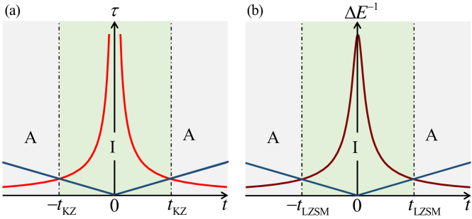
Figure 10: Adiabatic-impulse model (AIM) which relates the Landau-Zener-Stückelberg-Majorana (LZSM) with the Kibble-Zurek mechanism (KZM). In (a) we show the time dependence of the relaxation time $\tau_{\mathrm{r}}(t)$ of second-order phase transitions. The inclined blue lines at $\tau_{\mathrm{r}}=\left|t\right|$ give the moments of time $t_{\mathrm{KZ}}$, which separate the adiabatic (A) and impulse (I) stages of evolution. In (b), we plot the inverse energy-level gap $\Delta E^{-1}$ for a two-level system.

There are some difficulties in observing the time evolution of second-order phase transitions, and these are related to their rapid speed (sufficient range of quench time scales) or controlling and counting the defects. Then the quantum simulation can effectively be used by means of a convenient controllable quantum system.

Making use of the interrelation between the LZSM and KZM, this simulation was done recently with such diverse systems as an optical interferometer Xu et al. (2014b), a semiconductor charge qubit in a double quantum dot Wang et al. (2014), superconducting phase and transmon qubits Gong et al. (2016a), a single trapped ¹⁷¹Yb⁺ ion Cui et al. (2016, 2020), spin-1 Bose-Einstein condensate Damski and Zurek (2009); Anquez et al. (2016), and NMR based studies Zhang et al. (2017). These simulations correctly reproduced the main KZM results: the boundary between the adiabatic and impulse regions, the freeze-out phenomenon, and the dependence of the topological defect density on the quench rate.

Nowadays, the KZM is a general model that provides a description of the nonequilibrium dynamics and creation of topological defects such as strings, vortices, and domain walls. Here, using an analogy with the LZSM theory, these appear during symmetry-breaking phase transitions in the following systems: Ising chains Quan and Zurek (2010); Das (2010); Henriet and Hur (2016) and spin-1/2 XX and XY chains when the transverse field or anisotropic interaction is quenched Mukherjee et al. (2007); Divakaran et al. (2009); Roósz et al. (2014), graphene in a time-dependent electric field Fillion-Gourdeau et al. (2016), and biaxial paramagnet in an external magnetic field Zvyagin (2018). For deviations of realistic systems from the paradigmatic KZM, see for example  Gao et al. (2017).

Even though there are some studies on periodic driving, for example, Mukherjee and Dutta (2009); Setiawan et al. (2015); Dutta et al. (2015b); Kar et al. (2016); Higuera-Quintero et al. (2022), we note that in the context of phase transitions, the vast majority of research is devoted to the single-passage transition/quench. In quantum simulations of the KZM, as mentioned above, it is straightforward to realize double or even multiple passages. This introduces interference, in addition to the possibility of nonadiabatic transitions. This may become one of the new twists in the interrelation between LZSM physics and symmetry-breaking second-order phase transitions. Much like how the KZM for a single passage was used to describe the Big Bang, the respective development may be useful for speculating about the Big Bounce theory.

III.2 Rotating-wave approximation (RWA)

III.2.1 Multi-photon Rabi oscillations

Consider now the situation of resonant driving, with those parameters close to where the energy distance $\Delta E$ equals the photon energy $\hbar\omega$ or, more generally, close to the energy of $k$ photons, $\Delta E\sim k\hbar\omega$. The former (the single-photon resonant excitation) is critical for microscopic systems where there are electron paramagnetic (spin) resonance and nuclear magnetic resonance Rabi (1937). In this case, the amplitude $A$ is usually small, and the $k$-photon resonances appear within perturbation theory Shirley (1965); Krainov (1976); Krainov and Yakovlev (1980).

In contrast, for mesoscopic systems, the strong-driving regime is both accessible and important. Hence, we will first consider the solution of the Schrödinger equation for a weak driving, afterwards for a strong driving, and then finally the solution of the Bloch equation. These solutions are based on the RWA (also called secular approximation), where the terms that are quickly varying in time are neglected.

For weak resonant driving, with $A\ll\Delta$ and $\delta\omega\equiv\omega-\Delta E/\hbar\ll\omega$, the upper-level occupation probability exhibits Rabi oscillations [see e.g. Neilinger et al. (2016); Shevchenko (2019)]:

$$P_{\mathrm{up}}(t) = \overline{P_{\mathrm{up}}}(1-\cos\Omega_{\mathrm{R}}t),$$ (66a)

$$\Omega_{\mathrm{R}} = \sqrt{\Omega_{\mathrm{R0}}^{2}+\delta\omega^{2}}\text{, \ \ \ }\Omega_{\mathrm{R0}}=\frac{A\Delta}{2\hbar\Delta E}\text{, \ \ \ }\overline{P_{\mathrm{up}}}=\frac{1}{2}\frac{\Omega_{\mathrm{R0}}^{2}}{\Omega_{\mathrm{R0}}^{2}+\delta\omega^{2}}.$$ (66b)

Here, $\overline{P_{\mathrm{up}}}$ describes the time-averaged occupation probability; it is maximal in resonance at $\delta\omega=0$.

For stronger driving, one usually assumes $A\gg\Delta^{2}/\hbar\omega$, which corresponds to what we call the diabatic limit, with $\delta\ll 1$. This condition also means that the minimal energy distance $\Delta$ is small; we then, have $\Delta E\approx\left|\varepsilon_{0}\right|$. The solution of the Schrödinger equation can be obtained close to the $k$-th resonance, with

$$\delta\omega^{(k)}\equiv k\omega-\frac{\left|\varepsilon_{0}\right|}{\hbar}\ll\omega,$$ (67)

as in Refs. Henry and Lang (1977); Kmetic and Meath (1985); Lopez-Castillo et al. (1992),

$$P_{\mathrm{up}}^{(k)}(t) = \overline{P_{\mathrm{up}}^{(k)}}(1-\cos\Omega_{\mathrm{R}}^{(k)}t),$$ (68a)

$$\Omega_{\mathrm{R}}^{(k)} = \sqrt{\Omega_{\mathrm{R0}}^{(k)2}+\delta\omega^{(k)2}}\text{, \ \ }$$ (68b)

$$\Omega_{\mathrm{R0}}^{(k)} = \frac{\Delta}{\hbar}J_{k}\!\!\left(\frac{A}{\hbar\omega}\right)\text{, \ \ }$$ (68c)

$$\overline{P_{\mathrm{up}}^{(k)}} = \frac{1}{2}\frac{\Omega_{\mathrm{R0}}^{(k)2}}{\Omega_{\mathrm{R0}}^{(k)2}+\delta\omega^{(k)2}}.$$ (68d)

These describe multi-photon Rabi oscillations. Here, the Rabi frequency is modulated by the Bessel function of the first kind $J_{k}$. If the system’s parameters vary, we must take into account all the resonances:

$$\overline{P_{\mathrm{up}}}=\sum_{k}\overline{P_{\mathrm{up}}^{(k)}}.$$ (69)

We could study the moment of time $t_{\max}$, when the upper-level occupation reaches its maximum for the first time and the probability $P_{\mathrm{up}}^{(k)}(T_{\mathrm{d}})$ after the double passage of the avoided crossing (i.e., after a full period) in resonance Lopez-Castillo et al. (1992). From Eq. (68a), these are given by $t_{\max}=\pi/\Omega_{\mathrm{R}}^{(k)}$ and

$$P_{\mathrm{up}}^{(k)}(T_{\mathrm{d}})=1-\cos\left(2\pi\frac{\Delta}{\hbar\omega}J_{k}\left(\frac{A}{\hbar\omega}\right)\right).$$ (70)

In the next approximation, in the small parameter $\Delta$ (to be more precise $\Delta^{2}/A\hbar\omega\ll 1$ here), we can obtain the shift of the resonance frequency, which is known as the Bloch–Siegert shift Lopez-Castillo et al. (1992). Although for small $\Delta$ the resonance frequency for the first resonance ($k=1$) from Eq. (68d) is $\omega=\left|\varepsilon_{0}\right|/\hbar$, the resonance for larger $\Delta$ is given by Eq. (66a): $\omega=\Delta E/\hbar=\sqrt{\varepsilon_{0}^{2}+\Delta^{2}}/\hbar$. Hence, when either $\Delta$ is large or the frequency $\omega$ is small, the results of the RWA can be improved by adding the Bloch–Siegert shift and higher corrections (generalized Bloch–Siegert shift) Tuorila et al. (2010). See Refs. Abovyan and Kryuchkyan (2016); Sun et al. (2016); Wang et al. (2017); Huang et al. (2017); Saiko et al. (2018); Kohler (2018) for those cases beyond the RWA.

More generally, taking into account relaxation, the RWA for a periodically driven system is presented in Appendix B.2. This is considered for a generic periodic drive $\varepsilon(t)=\varepsilon_{0}+\widetilde{\varepsilon}(t)$, with $\widetilde{\varepsilon}(t)=A\cos\omega t$ as a particular case. The TLS is considered as being coupled to a dissipative environment, the impact of which is taken into account by introducing the relaxation and decoherence rates $\Gamma_{1,2}=T_{1,2}^{-1}$ Silveri et al. (2012, 2015). Then, the solution of the Bloch equations gives the upper-level occupation probability $P_{\mathrm{up}}$, which for the stationary case reads

$$\color[rgb]{0,1,0}\boxed{\color[rgb]{0,0,0}\overline{P_{\mathrm{up}}}=\frac{1}{2}\sum_{k=0}^{\infty}\frac{\Omega_{\mathrm{R0}}^{(k)2}}{\Omega_{\mathrm{R0}}^{(k)2}+\frac{\Gamma_{1}}{\Gamma_{2}}\left(k\omega-\left|\varepsilon_{0}\right|/\hbar\right)^{2}+\Gamma_{1}\Gamma_{2}},\color[rgb]{0,1,0}}\color[rgb]{0,0,0}$$ (71)

where

$$\Omega_{\mathrm{R0}}^{(k)}=\frac{\Delta}{\hbar}\frac{\omega}{2\pi}\int\limits_{0}^{2\pi/\omega}dt\exp\left[\frac{i}{\hbar}\int_{0}^{t}dt^{\prime}\widetilde{\varepsilon}\left(t^{\prime}\right)-ik\omega t\right].$$ (72)

These are quite general results that can be applicable to any driving $\widetilde{\varepsilon}\left(t\right)$. In particular, for $\widetilde{\varepsilon}\left(t\right)=A\cos\omega t$, we obtain the Rabi frequency (68c).

Role of the driving shape

Although most of this review is devoted to sinusoidal driving, we consider here the role of driving shape on the LZSM interference Blattmann et al. (2015). In general, equations like (71, 72) can be useful for describing any periodic perturbation $\widetilde{\varepsilon}\left(t\right)$, including multiharmonic drivings. Although the qualitative picture is similar for any periodic signal, the overall interference fringes can differ. This was studied for such pulses as triangular Xu et al. (2010), hyperbolic tangent and Gaussian Cao et al. (2010), rectangular Silveri et al. (2015); Shi et al. (2021), secant Zhao et al. (2018), and other ones Mukherjee et al. (2016); Xie (2018).

As a special and illustrative case, we now consider biharmonic driving Blattmann et al. (2015). This allows to study the effect of commensurate versus incommensurate driving frequencies Forster et al. (2015). It has been demonstrated that depending on the phase difference between its two components, bichromatic driving with commensurable frequencies may break time-reversal symmetry, which is visible in the Fourier transform of the LZSM interference pattern and which is useful for quantum simulation. Depending on the desired properties of the transitions, we can tailor the requested driving signal. We will return to this in the section on quantum control. Here, we illustrate this by referring to the development of the Lyapunov-based control method. In Ref. Cong et al. (2015), it was demonstrated that an ultrafast excitation can be gained by using a signal based on the Lyapunov control method, which is a design control method based on the Lyapunov indirect stability theorem.

Now, with the equations above, Eqs. (71) and (68c), we can plot the interferograms for sinusoidal driving, as shown in Fig. 11. Regarding the dependence of the time-averaged occupation of the upper diabatic level $\overline{P_{\mathrm{up}}}$ on the bias $\varepsilon_{0}$ and driving amplitude $A$, we can see that the resonances are along the lines $\left|\varepsilon_{0}\right|=k\hbar\omega$, and these are interrupted by the zeros of the Bessel functions, resulting in the CDT. The width of the resonances, as defined by Eq. (71), depends on the interrelation of the parameters; this is illustrated in the figure by varying the driving frequency $\omega$.

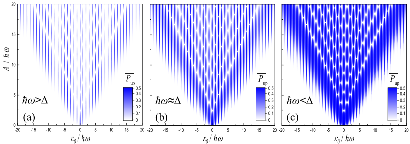
Figure 11: LZSM interferogram for different frequencies. For this, we took $\hbar\omega/\Delta=10$, $1.14$, $0.32$, for (a-c) and $\Gamma_{1}=0.1T_{\mathrm{d}}^{-1}$, $\Gamma_{2}=\Gamma_{1}/2$.

For strong driving, $A>\hbar\omega$, from Eqs. (71, 72), we arrive at Eq. (62). For this, we use the asymptotics of the Bessel functions and neglect the dissipation by considering the case when $T_{1}=T_{2}=\infty$. Importantly, we now see that two different theoretical approaches, the AIM and RWA, which we redeveloped in different parameter regimes, lead to the very same result: Eq. (62). Moreover, in the following subsections, we arrive at at the same result while presenting two other approaches.

III.2.2 Multi-photon transitions analyzed by the LZSM theory

It is well known that “an atom submitted to sufficiently intense radiation can absorb several incident photons and go from a discrete level $a$ to another discrete level $b$ located at a higher energy, at a distance equal to the sum of the energies of the absorbed photons. Such a process is called multi-photon absorption, the reverse process being multi-photon stimulated emission” Cohen-Tannoudji et al. (1998). The observation in the previous subsection demonstrates that multi-photon transitions are essential and appear consistently in different pictures, both within resonant RWA and within LZSM theory. In particular, from Eq. (71), we can see that the resonances take place at $k\hbar\omega=\left|\varepsilon_{0}\right|\approx\Delta E$.

Multi-photon processes have been studied in various systems: superconducting qubits Wallraff et al. (2003); Saito et al. (2004); Tornes and Stroud (2008); Shevchenko et al. (2012b), two-dimensional electron systems Zudov et al. (2006), atomic and molecular structures Arbó et al. (2010), Rydberg atoms Førre (2004); van Ditzhuijzen et al. (2009), TLSs in superconducting circuits Burin et al. (2014), quantum dots Giavaras and Tokura (2019a, b), and electromechanical systems Heinrich et al. (2010).

A TLS can be subjected to resonant driving with the energy of $k$ photons matching the distance between the energy levels $k\hbar\omega\approx\Delta E$; this induces a transition from one level to another. These can be described as the exchange of energy quanta (here, photons) with the oscillating driving field, which is known as photon-assisted tunneling (PAT); see, for instance, Ref. Li et al. (2013), where this was studied for a superconducting qubit. PAT was studied extensively for other various quantum systems with tunneling, especially for semiconductor nanostructures Platero and Aguado (2004), including driven quantum dots Mavalankar et al. (2016); Osika and Szafran (2017) and qubit-resonator dimers Zheng et al. (2021). Through a double quantum dot, PAT is described by the tunneling current defined by a formula analogous to Eq. (71) Stoof and Nazarov (1996); Gallego-Marcos et al. (2015).

Historically, the first experiments with PAT were performed on AC-driven Josephson contacts Tien and Gordon (1963). In this context, we can note the similarity and difference of the PAT (or, equivalently, multi-photon Rabi oscillations) and AC Josephson effect with the Shapiro steps, both of which appear for an irradiated superconducting tunnel junction. The former relates to the tunneling of electrons (quasiparticles) and results in steps in the current-voltage curve displaced in voltage by $k\hbar\omega/e$; the latter assumes the supercurrent response, which occurs as the Shapiro steps at voltages $k\hbar\omega/2e$ Nakamura et al. (2001). Both sets of resonances were observed experimentally and described theoretically in Boris and Krasnov (2015); Shaikhaidarov et al. (2022). In that study, it was demonstrated that the Shapiro steps and PAT states originate from Cooper-pair and quasiparticle currents; and if a JJ is subjected to an intense microwave signal, both sets of resonances can be observed in the current, changing both the voltage and microwave power Boris and Krasnov (2015); Snyder et al. (2018).

III.3 Floquet theory

It is natural to use the Floquet theorem for solving the Schrödinger equation for a periodically driven system. The theory based on this— Floquet theory—has been covered in many reviews Chu (1989); Grifoni and Hänggi (1998); Chu and Telnov (2004); Son et al. (2009); Shevchenko et al. (2010); Eckardt (2017); Rodriguez-Vega et al. (2021); Sen et al. (2021). We now consider this for our problem of describing the dynamics and stationary state of a driven TLS; the details are given in Appendix B.3.

For a time-dependent Schrödinger equation, Eq. (15), for the wave function $\left|\psi(t)\right\rangle$ with a periodic Hamiltonian $H(t)=H(t+T_{\mathrm{d}})$, we can use the Floquet theorem. Accordingly to this, the solution (so-called Floquet-state solution) is

$$\left|\psi(t)\right\rangle=\Sigma_{j=1,2}C_{j}\exp\left(-i\epsilon_{j}t/\hbar\right)\left|\Phi_{j}(t)\right\rangle,$$ (73)

where $\left|\Phi_{j}(t)\right\rangle$, is a periodic state, called the Floquet mode. The index $j=1,2$ appears because we are dealing with a two-dimensional Hilbert space. The real-valued $\epsilon{j}$ are called quasienergies, to reflect the formal analogy with a quasimomentum $\mathbf{k}$, which characterizes electron Bloch eigenstates in a periodic solid state Zel’dovich (1967, 1973); Averbukh and Perel’man (1985). The quasienergies are unique up to multiples of $2\pi n/T_{\mathrm{d}}$. It follows that these are the eigenstates in the problem

$$\color[rgb]{1,.5,0}\boxed{\color[rgb]{0,0,0}\left(H(t)-i\hbar\frac{d}{dt}\right)\left|\Phi_{j}(t)\right\rangle\equiv\mathcal{H}(t)\left|\Phi_{j}(t)\right\rangle=\epsilon_{j}\left|\Phi_{j}(t)\right\rangle.\color[rgb]{1,.5,0}}\color[rgb]{0,0,0}$$ (74)

The quasienergy states for time-dependent problems play a role analogous to the stationary states for time-independent problems.

Using the Floquet formalism allows us to reduce the problem of periodic perturbation to the stationary problem Shirley (1965); Barone et al. (1977); Ikeda et al. (2022), which is known as the Floquet Hamiltonian method Chu (1989); Chu and Telnov (2004). For this, one needs to expand the quasienergy function into a Fourier series, $\left|\Phi_{j}(t)\right\rangle=\Sigma_{n}e^{in\omega t}\left|\Phi_{j,n}\right\rangle$. Hence, the quasienergy states become expressed as a superposition of stationary states $\left|\Phi_{j,n}\right\rangle$, with energies equal to $\epsilon{j}+n\hbar\omega$. Using the Fourier series expansion, from the Schrödinger equation, we obtain the relation

$$\epsilon{j}\left|\Phi_{j,n}\right\rangle=\left(-\frac{\Delta}{2}\sigma_{x}-\frac{\varepsilon_{0}}{2}\sigma_{z}+n\omega\right)\left|\Phi_{j,n}\right\rangle-\frac{A}{2}\sigma_{z}\left(\left|\Phi_{j,n-1}\right\rangle+\left|\Phi_{j,n+1}\right\rangle\right).$$ (75)

Multiplying this to the left by $\left\langle\Phi_{i,m}\right|$, we obtain the matrix equation for the eigenvalues $\epsilon{j}$ and eigenfunctions $\left|\Phi_{j,n}\right\rangle$. Then, we truncate the matrix to solve the equation numerically, say, with $n$ ranging from $-50$ to $50$ Deng et al. (2016).

Close to the resonance, $\delta\omega^{(k)}\equiv k\omega-\left|\varepsilon_{0}\right|/\hbar\ll\omega$, the contribution of the nonresonant states can be neglected. This means using the RWA, for example, as in Autler and Townes (1955); Aravind and Hirschfelder (1984); Silveri et al. (2013). Then, the Floquet Hamiltonian consists just of the copies of

$$H_{\mathrm{RWA}}^{(k)}=\left(\begin{array}[]{cc}-\varepsilon_{0}/2&-\hbar\Omega_{\mathrm{R0}}^{(k)}/2\\ -\hbar\Omega_{\mathrm{R0}}^{(k)}/2&\varepsilon_{0}/2+k\hbar\omega\end{array}\right),$$ (76)

where the Rabi frequency $\Omega_{\mathrm{R0}}^{(k)}$ is the one defined in Eq. (68c). Diagonalization of this Hamiltonian produces the quasienergy difference, which we denote as $\hbar\Omega_{\mathrm{R}}^{(k)}$: $H_{\mathrm{RWA}}^{(k)\prime}=\sigma_{z}\hbar\Omega_{\mathrm{R}}^{(k)}/2$. This brings us to the same result as RWA; see Eq. (68b). Hence, Floquet theory in the secular approximation (i.e., in the RWA) gives us again the upper-level occupation probability in Eq. (68d) Son et al. (2009).

These RWA results are accurate, provided $\Delta/\hbar\omega\ll 1$. The higher-order terms can be obtained within the generalized van Vleck perturbation theory Hausinger and Grifoni (2010), resulting in a shift of the resonance frequency by

$$\delta_{k}=\frac{1}{2}\sum_{l\neq-k}\frac{\Omega_{\mathrm{R0}}^{(l)2}}{\varepsilon_{0}/\hbar+l\omega}.$$ (77)

This means that the resonances are situated at $\varepsilon_{0}=k\hbar\omega-\delta_{k}$, and that the Rabi frequency becomes $\delta_{k}$-shifted, $\Omega_{\mathrm{R}}^{(k)}=\sqrt{\Omega_{\mathrm{R0}}^{(k)2}+\left(\delta\omega^{(k)}-\delta_{k}\right)^{2}}$. Note that these formulas are calculated in the diabatic basis, while for the adiabatic basis, some modifications must be made Silveri et al. (2013).

In particular, consider the first-order correction from Eq. (77), which is $\delta_{1}=\Delta^{2}/2\varepsilon_{0}$. Then, we expect the first resonance at $\varepsilon_{0}=\hbar\omega-\Delta^{2}/2\varepsilon_{0}$ (where we can apply $\varepsilon_{0}=\hbar\omega$ in the right-hand-side). This matches the original Rabi approach. Indeed, from Eq. (66a), we have the resonances at $\hbar\omega=\sqrt{\Delta^{2}+\varepsilon_{0}^{2}}$, where the expansion gives $\varepsilon_{0}=\hbar\omega-\Delta^{2}/2\varepsilon_{0}$. Hence, generalized van Vleck perturbation theory gives the correction exactly consistent with the Rabi RWA, which is valid for small driving amplitudes Sambe (1973). For more about the resonance shift, termed AC Stark shift or Bloch-Siegert shift, see Autler and Townes (1955); Aravind and Hirschfelder (1984); Yan et al. (2017).

Because they are related to the Rabi frequency, the Floquet quasienergies can be visualized in experiments, known as Floquet spectroscopy. This was realized recently with qubits in cavities. In this case, the cavity is a superconducting microwave resonator and qubits are based either on superconducting circuits Silveri et al. (2013); Deng et al. (2015) or on double quantum dots Koski et al. (2018); Chen et al. (2021a). Other possible realizations include such systems as a strongly driven Anderson insulator Agarwal et al. (2017) or pumping in a Cooper pair sluice Russomanno et al. (2011). As a further development of the theory, this approach can be used to study the low-frequency limit Rodriguez-Vega et al. (2018), include the dissipation Henriet et al. (2014); Restrepo et al. (2016); Kohler (2017); Mori (2022) (Floquet-Markov theory), and considering multilevel systems Denisenko et al. (2010); Ganeshan et al. (2013); Satanin et al. (2014); Han et al. (2019, 2020); Munyaev and Bastrakova (2021); Zhou et al. (2021).

III.4 Driving fields in the quantum regime

Our approach above, in which the driving field is treated as a classical field and enters as $\varepsilon(t)$, is essentially the semiclassical approach. This takes place when the system of interest is described by the Schrödinger equation and a field satisfies classical Maxwell equations. In the other, fully quantum-mechanical approach, both the system and electromagnetic field are treated quantum mechanically. Importantly, semiclassical theory gives rise to results that are equivalent to those obtained from fully quantized theory in intense fields Aravind and Hirschfelder (1984); Grifoni and Hänggi (1998); Chu (1989). We discuss this below. For experimental realizations, see Nakamura et al. (2001); Saito et al. (2004); Wilson et al. (2007); Kervinen et al. (2019).

A TLS coupled to a quantum field is described by the Janes–Cummings Hamiltonian with driving:

$$\color[rgb]{1,.5,0}\boxed{\color[rgb]{0,0,0}H_{\mathrm{Q}}(t)=-\frac{\Delta}{2}\sigma_{x}-\frac{\varepsilon_{0}}{2}\sigma_{z}+\hbar\omega_{\mathrm{r}}a^{\dagger}a-g\sigma_{z}\left(a+a^{\dagger}\right)+\xi\left(a^{{\dagger}}e^{-i\omega t}+ae^{i\omega t}\right),\color[rgb]{1,.5,0}}\color[rgb]{0,0,0}$$ (78)

where $a$ and $a^{\dagger}$ are the annihilation and creation operators for photons in the electromagnetic field, $g$ is the coupling constant, $\xi$ describes the amplitude of the driving field, and the driving frequency $\omega$ is close to the resonator frequency $\omega_{\mathrm{r}}$. For example, for a flux qubit coupled to a transmission line resonator, the coupling constant is proportional to the persistent current in a flux qubit $I_{\mathrm{p}}$, which is the current constant in the resonator $I_{\mathrm{r0}}$, and the mutual inductance $M$: $g=MI_{\mathrm{p}}I_{\mathrm{r0}}$; the driving amplitude is defined by the amplitude of the applied microwave voltage $V_{A}$, the voltage constant in the resonator $V_{\mathrm{r0}}$, and a coupling capacitance $C_{0}$: $\xi=C_{0}V_{A}V_{\mathrm{r0}}$ Greenberg (2007); Shevchenko (2019). Note that the last term in Eq. (78) describes driving through the resonator; if the driving is through the qubit, this term would be proportional to $\sigma_{z}\cos\omega t$ Zhao et al. (2015).

Next, we need to get rid of the temporal dependence in the driving term with the transformation $U=\exp\left(i\omega ta^{\dagger}a\right)$, resulting in $H_{\mathrm{Q}}\rightarrow\widetilde{H}_{\mathrm{Q}}$, and to average this over the coherent states $\left|\alpha\right\rangle$ Aravind and Hirschfelder (1984); Sun et al. (2012). One way to define the coherent states is to assign them as the eigenstates of the annihilation operator, $a\left|\alpha\right\rangle=\alpha\left|\alpha\right\rangle$; it follows that the value $\alpha$ is given by the mean number of photons in the resonator: $\left\langle n\right\rangle=\left|\alpha\right|^{2}$. The resulting Hamiltonian $H=\left\langle\alpha\right|\widetilde{H}_{\mathrm{Q}}\left|\alpha\right\rangle$ becomes our quasiclassical qubit Hamiltonian $H(t)$ in Eq. (1), with the cosine bias with the amplitude $A=4\alpha g$ in Eq. (42), quod erat demonstrandum, which is one of the cornerstones of circuit quantum electrodynamics (QED).

Alternatively, one can show that $H_{\mathrm{Q}}(t)$ in matrix form is exactly reduced to the Floquet Hamiltonian $H_{\mathrm{F}}$ for an intense driving field Aravind and Hirschfelder (1984). For this, the annihilation and creation operators satisfy the following relations: $a\left|n\right\rangle=\sqrt{n}\left|n-1\right\rangle$ and $a^{\dagger}\left|n-1\right\rangle=\sqrt{n}\left|n\right\rangle$. Then, with $\Delta=0$, the Hamiltonian can be diagonalized exactly Cohen-Tannoudji et al. (1998); Nakamura et al. (2001); Saito et al. (2004); Wilson et al. (2007, 2010) with the eigenstates

$$\left|0,n\right\rangle=\left|0\right\rangle\otimes D\left(\widetilde{g}\right)\left|n\right\rangle\text{, \ \ }\left|1,n\right\rangle=\left|1\right\rangle\otimes D\left(-\widetilde{g}\right)\left|n\right\rangle\text{, where\ }D(\widetilde{g})=\exp\left(\widetilde{g}\left(a^{\dagger}-a\right)\right)\>\>\text{ and\ }\>\>\>\widetilde{g}=\frac{g}{\hbar\omega}.$$ (79)

These states are called the dressed-state basis; their eigenenergies are

$$E_{j,n}=n\hbar\omega-\frac{g^{2}}{\hbar\omega}+(-1)^{j}\varepsilon_{0}.$$ (80)

Here, $D$ is the displacement operator, the parameter $\widetilde{g}$ defines the strength of the coupling, while $j=0,1$ is attributed to the TLS, and $n$ to the number of photons in the cavity. Then, in this dressed-state representation, the matrix elements of the full Hamiltonian (with nonzero $\Delta$) coincide with the ones of the Floquet Hamiltonian $H_{\mathrm{F}}$, Eq. (215). When $E_{0,n+k}\approx E_{1,n}$, that is, when the $k$-photon resonance condition is met, $k\hbar\omega=\varepsilon_{0}$, the two dressed-states experience avoided-level crossing with the coupling (off-diagonal element) $\frac{1}{2}\Delta J_{k}(\alpha)$, resulting in $k$-photon Rabi oscillations with frequency $\Omega_{\mathrm{R}}^{(k)}=\Delta J_{k}(\alpha)/\hbar$, as above in the RWA.

Ultra-strong coupling regime

The picture above is in agreement with the semiclassical approach. However, there is a particular regime with very strong coupling and small photon numbers where some differences may appear Saiko et al. (2016); Ashhab (2017). To understand this, note that with the driving field in the quantum regime, when we consider strong driving, we mean large $A=4\alpha g$; but this can be reached with either a large coupling $g$ or a large number of photons $\left\langle n\right\rangle$. Accordingly, we can consider several limiting cases of the strong driving Li et al. (2013); Ashhab (2017); Bonifacio et al. (2020):

$$A=4\sqrt{\left\langle n\right\rangle}g\ \gg\ \hbar\omega\text{ \ }\leftrightarrow\text{ \ }\begin{cases}\widetilde{g}\ll 1,\>\>\>\text{ weak coupling with }\left\langle n\right\rangle\ggg 1\text{,}\>\>\>\>\>\>\>\>\>\>\>\>\>\>\\ \widetilde{g}\sim 1,\>\>\>\text{ (deep-)strong coupling with }\left\langle n\right\rangle\gg 1\text{,}\\ \widetilde{g}\gg 1,\>\>\>\text{ ultra-strong coupling with }\left\langle n\right\rangle\sim 1\text{.}\>\>\>\>\>\end{cases}$$ (81)

For all these regimes, the Rabi frequency in the quantum case, around the $k$-photon resonance, $k\hbar\omega=\varepsilon_{0}$, reads Ashhab (2017)

$$\Omega_{\mathrm{R,Q}}^{(k)}=\frac{\Delta}{\hbar}\left(2\widetilde{g}\right)^{k}\exp\left[-2\widetilde{g}^{2}\right]\sqrt{\frac{n!}{\left(n+k\right)!}}L_{n}^{k}\left(2\widetilde{g}^{2}\right),$$ (82)

where $L_{n}^{k}$ are the associated Laguerre polynomials. The numerical calculations in Ref. Ashhab (2017) demonstrate that the semiclassical dynamics is fully consistent with the quantum dynamics with the Rabi frequency in Eq. (82), but only for small coupling $\widetilde{g}$ and large photon number $n$. In the ultra-strong coupling regime, from Eq. (82), where the fully quantum approach provides decaying oscillations because of quantum fluctuations and where the Rabi frequency deviates from the result of the semiclassical approach.

Dressed-states and interferometry for systems which are either doubly driven or driven by a chirped microwave

The notion of dressed-states, which we just considered for the quantum driving fields, appears when describing driving systems in a different context. Here, we mean the case when both the Hamiltonian of a TLS and driving can be rewritten as an effective TLS; hence describing entangled light-matter states, which are also known as dressed-states Magazzù et al. (2018); Chang et al. (2020). This notion appears because the qubit is now dressed by the driving field. This approach is useful for systems that do not have avoided energy-level crossing, or where their energy-level spacing does not depend on the external bias parameters Gong et al. (2016b). Here, a typical case with these two properties is a transmon qubit Fink et al. (2009); to make its effective energy levels controllable and, in particular, for realizing the LZSM regime, this can be achieved by using either a chirping field or a second signal Garraway and Stenholm (1992a); Gauthey et al. (1997); Vitanov et al. (2001); Sun et al. (2011); Silveri et al. (2015); Garraway and Perrin (2016); Gong et al. (2016b).

To illustrate dressed-states and interferometry, consider now a doubly driven TLS, described by the “pump-probe” Hamiltonian, for example Wen et al. (2020),

$$H_{\mathrm{pp}}=-\sigma_{x}\Delta\cos\omega_{\mathrm{probe}}t+\frac{\sigma_{z}}{2}\left(\hbar\omega_{10}+\delta\cos\omega_{\mathrm{pump}}t\right).$$ (83)

This corresponds to a TLS with distance between the energy levels equal to $\hbar\omega_{10}$ and driven by two signals, with amplitudes proportional to $\Delta$ and $\delta$, assuming $\omega_{\mathrm{pump}}\ll\omega_{\mathrm{probe}}$. Using the transformation $U=\exp\left(-i\omega_{\mathrm{probe}}\sigma_{z}t/2\right)$ and the RWA lead to the Hamiltonian (1) with

$$\varepsilon(t)=\hbar\left(\omega_{10}-\omega_{\mathrm{probe}}\right)+\delta\cos\omega_{\mathrm{pump}}t.$$ (84)

Now, after arriving at the pseudo-spin Hamiltonian for our driven system (which we can now call the dressed Hamiltonian), we can understand the two options above.

First, we apply two signals, the pump (dressing) signal and probe signal, obtaining the bias (42) with $\varepsilon_{0}=\hbar\left(\omega_{10}-\omega_{\mathrm{probe}}\right)$ (for a transmon, this is controlled by the DC magnetic flux, changing $\omega_{10}$), $A=\delta$, and $\omega=\omega_{\mathrm{pump}}$ Silveri et al. (2015).

Second, we do not have a second signal, $\delta=0$, while the “probe” frequency is time dependent, $\hbar\omega_{\mathrm{probe}}(t)\rightarrow\varepsilon_{0}+A\cos\omega t$; see Ref. Gong et al. (2016b) for chirping with triangular pulses, Refs. Childress and McIntyre (2010); Blattmann et al. (2014); Ono et al. (2019) for sinusoidal frequency modulation, and Refs. Saiko et al. (2007, 2014, 2019); Wang et al. (2021) for the impact of bichromatical driving.

LZSM spectroscopy of multilevel systems

For a multilevel system, a similar dressing can also be applied to create an avoided-level structure of energy levels Mi et al. (2018); Shevchenko et al. (2018). For this, we apply the driving signal with frequency $\omega_{\mathrm{d}}$ close to the energy-level separation $\Delta_{0}$ at $\varepsilon=0$, to obtain the dressed avoided-level gap $\Delta\approx(\Delta_{0}-\hbar\omega_{\mathrm{d}})\ll\Delta_{0}$. Then, the dressed energy levels are related to the bare ones as $\widetilde{E}_{i}\approx E_{i}\pm\hbar\omega_{\mathrm{d}}$. As a result, in addition, this dressing can significantly increase the distance between the lower two energy levels and upper ones, providing an instrument for creating controllable TLSs out of multilevel ones. In such case, note that features of the TLS’s spectrum, such as the curvature of its energy levels, essentially depend on the entire energy spectrum of the bare multilevel system Mi et al. (2018); Shevchenko et al. (2018). Hence, the LZSM interferogram of the effective dressed TLS is a convenient tool for the spectroscopy of multilevel systems.

III.5 Impact of dissipation and temperature

Any real quantum system is coupled with the environment, and for mesoscopic systems, it is particularly important to include dissipation. Many authors study the impact of temperature, relaxation, and decoherence on the dynamics of TLSs Leggett et al. (1987); Grifoni and Hänggi (1998). The general approach is to start from the Liouville–von Neumann equation for the density matrix $\rho_{\mathrm{tot}}$ of the system, here comprising of our quantum system and the dissipative environment

$$\frac{d}{dt}\rho_{\mathrm{tot}}(t)=-\frac{i}{\hbar}\left[H_{\mathrm{tot}}(t),\rho_{\mathrm{tot}}(t)\right].$$ (85)

The total Hamiltonian, $H_{\mathrm{tot}}=H+H_{\mathrm{env}}+H_{\mathrm{int}}$, consists of our system’s part $H$, the environment Hamiltonian $H_{\mathrm{env}}$, and the interaction between them $H_{\mathrm{int}}$, for example, Nalbach and Thorwart (2009). Provided the coupling is weak, the environment can be represented as a set of harmonic oscillators with a coupling linear in the oscillator coordinates. Within this “spin-boson” model, the environment is characterized by the Hamiltonian $H_{\mathrm{env}}=\sum\hbar\omega_{i}b_{i}^{{\dagger}}b_{i}$ with the frequencies $\omega_{i}$ and annihilation operators $b_{i}$; a bosonic reservoir can represent phonons if our system is coupled with a crystal lattice. The general form of the interaction is given by $H_{\mathrm{int}}=-\frac{1}{2}\mathcal{S}\sum\hbar\lambda_{i}(b_{i}+b_{i}^{{\dagger}})$, with $\mathcal{S}$ representing a spin operator; usually, $\mathcal{S}=\sigma_{z}$ Kayanuma and Nakayama (1998); Saito and Kayanuma (2002); Chen et al. (2015); Wertnik et al. (2018); Lambert et al. (2019, 2020); Funo et al. (2021).

The environment is described by the spectral density function $J(\omega)=\pi\sum\lambda_{i}^{2}\delta(\omega-\omega_{i})$ Leggett et al. (1987). At small energies, this is characterized by a power-law dependence and can be further approximated by introducing the cutoff frequency $\omega_{\mathrm{c}}$: $J(\omega)=\alpha\omega(\omega/\omega_{\mathrm{c}})^{s-1}\exp\left(-\omega/\omega_{\mathrm{c}}\right)$, where the dimensionless parameter $\alpha$ defines the strength of the coupling and the power law is described by $s$, with $s=1$ for the ohmic environment Ao and Rammer (1989, 1991). For nonohmic cases, see Leggett et al. (1987). As a simple approach, we can consider the environment being modeled as only one (finite-temperature) harmonic oscillator Saito et al. (2007); Ashhab (2014); Malla and Raikh (2018).

Tracing out the environment’s degrees of freedom, we can obtain a master equation for the reduced density matrix $\rho(t)$ of our system, which can be written as the Lindblad equation (also known as the Lidblad-Gorini–Kossakowski–Sudarshan equation, Chruściński and Pascazio (2017))

$$\color[rgb]{1,.5,0}\boxed{\color[rgb]{0,0,0}\dot{\rho}=-\frac{i}{\hbar}\left[H(t),\rho\right]+\sum_{k}\left(L_{k}\rho L_{k}^{{\dagger}}-\frac{1}{2}L_{k}^{{\dagger}}L_{k}\rho-\frac{1}{2}\rho L_{k}^{{\dagger}}L_{k}\right).\color[rgb]{1,.5,0}}\color[rgb]{0,0,0}$$ (86)

Different channels of relaxation are described by the Lindblad operators $L_{k}$. Note that Lindblad equation is correct under certain conditions such as:

• separability (no correlations between the system and its environment at $t=0$),

• Born approximation (environment is static despite interaction with quantum system, and weak coupling between quantum system and environment),

• Markov approximation (time scale of decay is much shorter than the smallest characteristic time of the system),

• secular approximation (all fast rotating terms in the interaction picture can be neglected).

For the limitations of the Lindblad equation, see Teixeira et al. (2021).

In particular, for a TLS, the impact of the environment results in relaxation and dephasing, as described by $L_{\mathrm{relax}}=\sqrt{\Gamma_{1}}(\sigma_{x}-i\sigma_{y})/2$ and $L_{\phi}=\sqrt{\Gamma_{\phi}/2}\sigma_{z}$. Instead of the relaxation rates, we can use the respective times: $T_{1}=\Gamma_{1}^{-1}$ and $T_{\phi}=\Gamma_{\phi}^{-1}$. Then, the Lindblad equation is reduced to the Bloch equations for the components of the Bloch vector $\mathbf{s}=\text{Tr}(\mathbf{\sigma}\rho)$; writing the Hamiltonian in the form $H=-\mathbf{B\cdot\sigma}/2$, with the effective “magnetic” field $\mathbf{B}$, these read as

$$\frac{d}{dt}\mathbf{s=-B\times s-}\frac{1}{T_{1}}\left(\mathbf{s}_{\|}\mathbf{-s}_{\|}^{\mathrm{eq}}\right)-\frac{1}{T_{2}}\mathbf{s}_{\bot},$$ (87)

$$T_{2}^{-1} = \frac{1}{2}T_{1}^{-1}+T_{\phi}^{-1}\text{, \ \ }\>\>\>\>s_{z}^{\mathrm{eq}}=\tanh(\Delta E/2k_{B}T).$$ (88)

Importantly, the Bloch equations are obtained based on the qubit eigenstates Krzywda and Cywiński (2021) (see also Xu et al. (2014a)). In particular, this assumes a relaxation to the ground state at low temperatures. Thus, the Hamiltonian $H(t)$ in the Lindblad and Bloch equations should be written in the representation of the adiabatic basis. The diagonalization of the Hamiltonian is done by a rotation on the angle $\eta$. The relaxation rates are related to the spectral density Makhlin et al. (2001) and depend on the energy offset $\varepsilon_{0}$ and temperature $T$

$$\Gamma_{1}=\pi\alpha\sin^{2}\eta\frac{\Delta E}{\hbar}\coth\frac{\Delta E}{2k_{B}T}\text{, \ \ }\>\>\>\>\Gamma_{\phi}=\pi\alpha\cos^{2}\eta\frac{2k_{B}T}{\hbar}.$$ (89)

The Bloch equations can be extended to a multilevel system Shimshoni and Gefen (1991); Gefen and Thouless (1987)

$$\dot{\rho}_{ii}(t) = -\frac{i}{\hbar}\left[H(t),\rho\right]_{ii}-\frac{\rho_{ii}(t)-\rho_{ii}^{\mathrm{eq}}(t)}{T_{1,i}},$$ (90a)

$$\dot{\rho}_{ij}(t) = -\frac{i}{\hbar}\left[H(t),\rho\right]_{ij}-\frac{\rho_{ij}(t)}{T_{2,ij}},\text{ \ \ }i\neq j\text{.}$$ (90b)

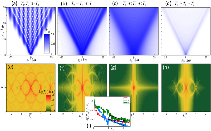
Figure 12: Impact of dissipation and dephasing on interferograms and tomograms. The upper panels present the LZSM interferograms and the lower panels their respective 2D Fourier transforms also known as tomograms. These interferograms and their tomograms are demonstrated in several cases: (a) and (e) low relaxation and dephasing, $T_{1}=10T_{\mathrm{d}}$, $T_{2}=20T_{\mathrm{d}}$; (b) and (f) low relaxation and the dephasing time comparable with the driving period, $T_{1}=10T_{\mathrm{d}}$, $T_{2}=0.5T_{\mathrm{d}}$; (c) and (g) weak relaxation and strong dephasing, $T_{1}=10T_{\mathrm{d}}$, $T_{2}=0.1T_{\mathrm{d}}$; and (d) and (h) both the relaxation time and the dephasing time comparable with the driving period, $T_{1}=0.25T_{\mathrm{d}}$, $T_{2}=0.5T_{\mathrm{d}}$. For all panels, the driving frequency is $\omega=1.14\Delta/\hbar$. The inset (i) shows that fitting the linear part of the dependence can be used for defining the decoherence time $T_{2}$.

Therefore, the most straightforward approach to demonstrate the impact of both dissipation and temperature is to solve the Bloch equations; see this also in Refs. Kayanuma (1993); Zueco et al. (2008); Nalbach and Thorwart (2009); Scala et al. (2011); Whitney et al. (2011); Orth et al. (2013); Xu et al. (2014a); Dai et al. (2022). In Fig. 12, we present the interferograms for different relaxation and dephasing rates and their Fourier images. In panel (a), we show the case of low dissipation and relaxation rates, in which all the resonances are distinguishable. In panel (b), we show the case of the average dephasing regime, which we also refer to as the double-passage regime, when several passages occur before dephasing dominates, which leads to merging resonances into lines.

The next regime is with large dephasing, which is shown in panel (c), where dephasing dominates over excitation and resonances merge into one region $A>|\varepsilon|$. Panel (d) presents the strong relaxation case when relaxation dominates over excitations. The characteristic pattern for this case is the peak of probability near $(\varepsilon_{0}=0,A=0)$, where an increasing in the driving amplitude results in the resonances disappearing.

Dissipative LZSM transitions were studied for quantum dots Fouokeng et al. (2014); Ota et al. (2017); Huang and Hu (2021), superconducting qubits Gramajo et al. (2019), and molecular nanomagnets that include the high-spin case Calero et al. (2005); Vogelsberger and Garanin (2006); Földi et al. (2008). The transition in a system subject to continuous measurement was considered in Ref. Haikka and Mølmer (2014). When the environment can be treated as a continuum of states, LZSM transitions can be formulated within the open-multistate model Dodin et al. (2014). The impact of dissipation on CDT is the suppression of those processes Hausinger and Grifoni (2010).

III.6 Rate equation

The master equation which describes a TLS can be written in the form of a rate equation. (This was not considered in Shevchenko et al. (2010), but this approach is also useful and important.) Consider here the microscopic analysis of the dynamics of a TLS based on the rate equation and adding classical noise to model decoherence Berns et al. (2006). Details are presented in the Appendix B.4.

First, we calculate the transition rate $W$ for a bias $\varepsilon(t)=\varepsilon_{0}+A\cos\omega t+\delta\varepsilon(t)$, in the presence of classical noise $\delta\varepsilon(t)$. For concreteness, we present the derivations and results for harmonic driving. This approach can be used for any other periodic driving, such as sawtooth-like and biharmonic ones Rudner et al. (2008); Berns et al. (2008); Cao et al. (2013).

Then, the averaging over $\delta\varepsilon(t)$ using the white-noise model gives the rate of transitions between the TLS states

$$W=\frac{1}{2}\sum_{n=-\infty}^{\infty}\frac{\Gamma_{2}\Delta_{n}^{2}}{\left(\varepsilon_{0}/\hbar-n\omega\right)^{2}+\Gamma_{2}^{2}},$$ (91)

where the splitting is modulated with the Bessel function, $\Delta_{n}=\Delta J_{n}(A/\hbar\omega)$ and $\Gamma_{2}=T_{2}^{-1}$ is the decoherence rate Du et al. (2010, 2013a).

Next, we construct the rate equation, which includes possible transitions between the states, with rate $W$, and relaxation, with rate $\Gamma_{1}=T_{1}^{-1}$. From the stationary solution of the rate equation, we obtain

$$P_{+}=\frac{W}{2W+\Gamma_{1}}\text{.}$$ (92)

The summation of all possible resonances gives us exactly the same solution as the one above: Eq. (71). This derivation of the formula (71) reveals its robustness.

The formalism presented here has the advantage that it is straightforward to be generalized for multilevel systems Wen et al. (2009). For a system with $N$ energy levels, we must solve a system of $N$ rate equations (like we do for a TLS in Appendix B.4) to describe the transitions between levels $i$ and $j$ with the rates $W_{ij}$, given by Eq. (91), replacing the splitting $\Delta\rightarrow\Delta_{ij}$ and offsets from them $\varepsilon_{0}\rightarrow\varepsilon_{ij}$. This approach was developed and applied to multilevel systems, including the ones based on superconducting qubits Wen et al. (2010); Du and Yu (2010); Wang et al. (2010); Chen et al. (2011) and double quantum dots (DQD). Chatterjee et al. (2018); Liul and Shevchenko (2022).

III.7 Quantum phase tomography

The Fourier transform is a useful tool for analyzing different periodic patterns. In the case of LZSM interferograms, the Fourier transform results in a highly ordered structure of one-dimensional arcs Berns et al. (2008). Because the Fourier image gives the structured mapping of the interferograms, it presents the tomographic imaging and the respective graphs give rise to a technique called quantum phase tomography Rudner et al. (2008). This approach gives additional information about the physical processes in a driven quantum system and is useful for defining system parameters, including for probing the dephasing mechanisms Rudner et al. (2008); Cao et al. (2013).

Having an analytical expression for $\overline{P_{\mathrm{up}}}$, we can use the continuous 2D Fourier transformation

$$P_{\mathrm{FT}}(k_{\varepsilon},k_{A})=\int\!\!\!\!\int_{-\infty}^{\infty}\overline{P_{\mathrm{up}}}(\varepsilon_{0},A)\exp\left[{-ik}_{\varepsilon}\varepsilon_{0}-ik_{A}A{)}\right]d\varepsilon_{0}dA,$$ (93)

where $k_{\varepsilon}$ and $k_{A}$ are the reciprocal-space variables corresponding to the variables $\varepsilon_{0}$ and $A$, respectively. In the case when the matrix of the data is given instead by a formula for $\overline{P_{\mathrm{up}}}$, we can use the discrete 2D Fourier transform. In the lower panels of Fig. 12, we present the tomograms related to the interferograms in the upper panels; these were calculated by the discrete Fourier transform of the data for the interferograms. We can see that the relaxation suppresses the low-frequency resonance curves; when increasing the relaxation rate, only the main curve (with $l=1$) survives, as can be seen in Fig. 12(h). Note that the vertical and horizontal lines of increased $P_{\mathrm{FT}}$ along the axes, especially at $k_{\varepsilon}=0$ and $k_{A}=0$, are artifacts because of the finite size of the interferograms.

The overall tomograms in Fig. 12(e-h) are lemon-shaped structures formed by the 1D sinusoids of the form

$$k_{A}(k_{\varepsilon})=\pm\frac{2l}{\omega}\sin\left(\frac{\omega k_{\varepsilon}+2\pi l^{\prime}}{2l}\right),$$ (94)

with $l=1,2,3,...$, $l^{\prime}=0,1,2,...$, and $l^{\prime}<l$. This can be seen by either analysis of the phase acquired during the periodic evolution Rudner et al. (2008) or by directly transforming Eq. (71) Forster et al. (2014); Blattmann et al. (2015). From the lower panels in Fig. 12, we can see how relaxation and dephasing impact the Fourier images. With low relaxation and decoherence rates, there are many resonances in panel (e). From panels (f) and (g), we can see that increasing the dephasing rate leads to increasing the slope rates along the $|k_{\varepsilon}|$ axis. Then, when we compare Fourier images on panels (f) and (h), we can see that for the same dephasing rate, increasing the relaxation rate leads to the disappearance of the higher resonances. In panel (i), we show the cross-sections of panels (f,g,h) along $k_{A}=0.85$; the slopes are given by the dephasing rates, as shown by the dashed lines. Note that in this panel, this is very noisy because of resonances and artifacts; to better see the slopes, one can consider the response along the resonance lines, as in Forster et al. (2014).

From Eqs. (91-92), we can find that the slope of the Fourier image is proportional to the decoherence rate:
$\ln P_{\mathrm{FT}}\propto-\Gamma_{2}|k_{\varepsilon}|$ Rudner et al. (2008). This is demonstrated as the inset, Fig. 12(i). This observation provides a convenient tool for obtaining the decoherence rate without additional measurement or fitting Cao et al. (2013); Gonzalez-Zalba et al. (2016). If this theory accounts for inhomogeneous broadening $\Gamma_{2}^{\ast}$, this results in

$$\ln P_{\mathrm{FT}}(k_{\varepsilon},k_{A}({\varepsilon}))\propto-\Gamma_{2}|k_{\varepsilon}|-\Gamma_{2}^{\ast 2}k_{\varepsilon}^{2}/2,$$ (95)

where $k_{A}(k_{\varepsilon})$ is defined by the relation Eq. (94) Forster et al. (2014). In addition to $\Gamma_{2}$, this provides a convenient tool for defining $\Gamma_{2}^{\ast}$, most importantly without any additional measurements, such as spin-echo experiments Cao et al. (2013).

Hence, the Fourier transform provides a useful tool, quantum-phase tomography, providing an additional visualization of the interference and the system parameters, such as the decoherence rate. This methodology can be further developed and applied to other systems, specifically for bichromatic driving Forster et al. (2015) and multilevel systems Berns et al. (2006); Liul and Shevchenko (2022).

III.8 Comparison of different methods

	Numerical ODE	Numerical QuTiP	Floquet method	RWA	Optimized RWA	AIM
$(\varepsilon_{0},A)$	3144	2050	1300	16.4	4.7	9.4
$(\varepsilon_{0},\omega)$	1400	1241	774	9.3	4	8.6

Table 3: Relative efficiency of different methods. This is quantified with the time (in seconds) needed to calculate the respective interferograms shown in Fig. 13. The first line relates to the interferograms in the coordinates $(\varepsilon_{0},A)$ and the second line to the coordinates $(\varepsilon_{0},\omega)$. The numbers in the table were obtained using an eight-core CPU Intel 10875H using eight threads.

Above we have considered in detail different methods for describing driven quantum systems. Now, we would like to compare these different approaches; see also Ashhab et al. (2007). We summarize their key aspects and then compare them by computing the interferograms.

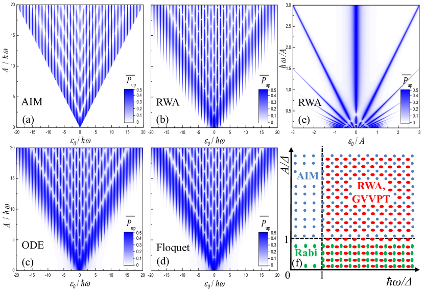
Figure 13: LZSM interferograms calculated by different methods. (a-d) and (e) present the time-averaged upper-level occupation probability as a function of the energy offset $\varepsilon_{0}$, the driving amplitude $A$ for (a-d) and the driving frequency $\omega$ for (e). Comparison between the regions of validity for different methods with small relaxation and dephasing rates (f). The methods used are the adiabatic-impulse model (AIM) (blue circles in panel (f)), rotating-wave approximation (RWA), and the second approximation by the Floquet method given by the generalized Van-Vleck perturbation theory (GVVPT), which has the same region of validity (red ovals in panel (f)). Numerical solution of the ordinary differential equations (ODE), and the Floquet approach can be applicable everywhere. Also, panel (f) demonstrates the region of validity for the Rabi oscillations method (green ovals).

Numerically solving the Schrödinger or Lindblad equation

This method is the most commonly used because it is based on the integration of a system of differential equations. This gives the best-quality results and can be used in all range of parameters. We compare all other methods with this one, because the numerical integration can be performed accurately. However, the numerical integration has one significant disadvantage: it needs considerable computing power, so it requires considerable CPU time to compute interferograms. We use the numerical solution based on the modified Runge-Kutta method, which is a standard approach for solving systems of ordinary differential equations (ODE) in Python.

Numerically solving using QuTiP

The QuTiP (Quantum Toolbox in Python) framework Johansson et al. (2012, 2013); Shammah et al. (2018) is a very useful tool to calculate the dynamics of quantum systems. We need only to introduce a Hamiltonian and set of parameters; as a result, we have the full evolution of the system (all terms of the density matrix, in all the defined moments of time) or, alternatively, the averaged value of population of a certain level. This library also has a detailed manual and many different solvers.

Floquet method

This approach can be used only for periodic Hamiltonians and is based on the Floquet theorem. The Floquet method is faster than the direct numerical solution, but slower than other analytical methods. Importantly, relaxation and dephasing can be included. This method is analogous to a decomposition on eigenfunctions in methods of mathematical physics.

Rotating-wave approximation (RWA)

The RWA corresponds to the first term in a Floquet formalism by the small distance between levels $\Delta\ll\omega,\varepsilon$. It is the most commonly used analytical method because it combines adequate accuracy with a moderate need in computing power. Here, for calculating interferograms, the range of application is limited by the overlap of resonances, which occurs at increasing relaxation and dephasing or decreasing driving frequency. In the simplest approach, we can use the formula Eq. (71), which assumes calculating a number of terms in each point. However, if we take a few close resonances only, that is, with $k$ close to the resonance condition $\varepsilon_{0}=k\hbar\omega$, this significantly speed-up the calculation; this approach can be called optimized RWA.

Adiabatic-impulse model (AIM)

The Adiabatic-impulse model can provide interferograms in different bases. This is generally done neglecting relaxation and decoherence; thus the time-averaged result obtained by this method depends on the initial condition. This correctly gives the location of the resonances; but between them this method may give different values from those obtained using more precise numerical calculations, which is a result of not including relaxation and dephasing. This means that the time-averaged result depends on the initial condition; but when we use the ground-state initial condition in this AIM and small dissipation in other methods, then the AIM gives the correct result. The range of usability of this method is defined by a high amplitude of excitation $A>\Delta$, which is needed for the adiabatic evolution between transitions. The second limitation is the times of the transition process: $T_{\text{d}}/2>(\tau_{\text{relax}}+\tau_{\text{jump}})$. See the transition times described in paragraph II.3.2.

Interferograms and time of calculation

We illustrate our conclusions in Fig. 13 and table 3. First, in Fig. 13: (a,b,c,d), we present the interferograms using the coordinates $(\varepsilon_{0},A)$; and in (e) using $(\varepsilon_{0},\omega)$. Even the former shows not so many differences, and these become even less for the latter in (e). For the calculations, we chose the driving frequency $\hbar\omega/\Delta=1.14$ and the relaxation rates for (b-d), $\Gamma_{1}=0.1T_{\mathrm{d}}^{-1}$ and $\Gamma_{2}=\Gamma_{1}/2$. Note that the adiabatic-impulse model in (a) is valid under the condition $A>\varepsilon_{0}$, with no relaxation and decoherence included. The RWA in (b) provides a result more similar to the numerical solution in (c), except the shifting of the resonances when increasing the driving amplitude, here in the region $A<\varepsilon_{0}$.

In table 3, as a quantitative measure of the efficiency, we have chosen the time needed to compute the interferograms. For this, we used an eight-core CPU Intel 10875H using eight threads. Calculations were performed as in Fig. 13, with 401 points in each axis. Note that the most significant impact on calculation time is given by the number of points, while the dependence on other parameters vary for different methods. As we see from table 3, the analytical methods are much faster than the numerical calculations, with a difference of about two orders of magnitude in calculation time. However, the numerical calculations is more flexible and can be easily used for more complicated systems, including many levels, adding noise, and so forth. For describing the time-averaged occupation probability, the most convenient method is the RWA. For describing the dynamics, one of the most illustrative methods is the adiabatic-impulse model, but it is limited by the time of the transition process; for more related information, see Sec. II.3.2.

IV Interferometry

The interference in a driven two- or multi-level system is essentially defined by the problem parameters. It is important for applications to demonstrate this through calculations and to formulate recipes of how to extract not only the quantum system parameters from the interferograms, but also the information about systems coupled with them, as well as about the dissipative environment Shytov et al. (2003); Yang et al. (2017).

Although we have given a detailed description of various systems with LZSM interference, we display the diversity of these, presenting several systems in Fig. 14. (Please note that the choice of works and figures for Fig. 14 are used only for illustrative purposes, while many other works are analyzed below and throughout this review paper.) A detailed description of Fig. 14 follows.

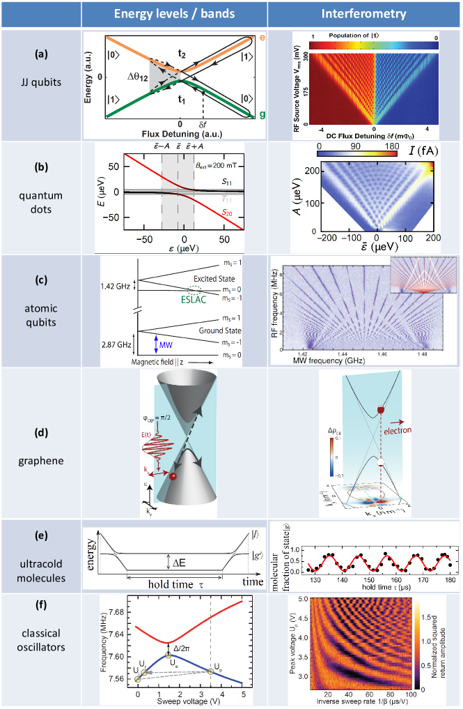
Figure 14: LZSM interferograms in different systems. See the extended explanation in the text for a detailed description. Figure (a) is reprinted from Berns et al. (2006) with permission; copyright (2006) by APS. Figure (b) is reprinted from Forster et al. (2014) with permission; copyright (2014) by APS. Figure (c) is reprinted from Childress and McIntyre (2010) with permission; copyright (2010) by APS. Figure (d) is reprinted from Heide et al. (2018) with permission; copyright (2018) by APS. Figure (e) is reprinted from Mark et al. (2007b) with permission; copyright (2007) by APS. Figure (f) is reprinted from Seitner et al. (2016) with permission; copyright (2016) by APS.

Extended explanation of Fig. (14):

(a) Superconducting circuits

Although JJ-based quantum superconducting circuits are diverse, we would like to illustrate the work on these systems with Ref. Berns et al. (2006). A superconducting flux qubit, also called a persistent-current qubit, was realized as a niobium (but it could also be aluminum) superconducting loop with three JJs. The basis states are created by a persistent current flowing either clockwise or in the counterwise direction. Strong driving by an AC magnetic flux induces transitions between the two states. In Ref. Oliver et al. (2005), these qubit states were read out with an outer DC-SQUID, a sensitive magnetometer that distinguishes the flux generated by the persistent currents. Up to 20-photon transitions were observed, with an impressive increase up to 45-photon transitions in Ref. Berns et al. (2006). The energy-level distance was controlled by a DC magnetic flux; the tunneling amplitude was rather small, $\Delta\simeq 13$ MHz$\cdot h$, and the driving frequency $\omega/2\pi=0.27~{}\mathrm{GHz}\gg\Delta/h$.

(b) Quantum dots

These are based on electrons localized in semiconductor low-dimensional systems. Specifically, a two-electron charge qubit, which is defined in a lateral double quantum dot, is considered in Ref. Forster et al. (2014). The source and drain leads, tunnel-coupled with dots, allow current flow by single-electron tunneling. This current is used to detect the properties of the driven double quantum dot (DQD) device. The charge qubit is formed by the singlet states $S_{11}$ (one electron in each dot) and $S_{20}$ (two electrons in the left dot). The source-drain current is proportional to the occupation probability of $S_{20}$. The three triplets $T_{11}$ are hindered by a Pauli-spin blockade; however, blockade is lifted using an on-chip nanomagnet to quickly initialize the qubit. In the energy diagram, the singlets (the qubit states) are represented as black and red lines; the triplets, which are Zeeman split, are shown as gray lines. The interdot coupling is $\Delta\simeq 3.1$ GHz$\cdot h$, and the energy detuning $\varepsilon$ is defined by a DC+AC gate voltages $\varepsilon(t)=\overline{\varepsilon}+A\cos\omega t$. The driving frequency for the interferogram shown is $\omega/2\pi=2.5~{}$GHz, which is smaller than $\Delta/h$.

(c) Atomic qubits (impurity or donor based)

These may involve electrons, holes, and/or nuclear spins in impurities within silicon, diamond, or other materials. For illustration purposes, we now consider an NV center in diamond, which consists of a substitutional nitrogen atom replacing a carbon atom and neighboring one vacancy. Its electronic ground state has a spin $S=1$, which, in the absence of a magnetic field, has the spin singlet sublevel $m_{s}=0$ situated $2.87$ GHz below the $m_{s}=\pm 1$ two-fold-degenerate triplet sublevels. The optically excited state has the zero-field splitting $1.42$ GHz. These can be further changed by the magnetic field. We illustrate this with an energy diagram displaying the excited-state level anticrossing (ESLAC) and the interferogram from Ref. Childress and McIntyre (2010). The system was doubly driven by a microwave and rf signals, resulting in characteristic dressed-state interference fringes. This was displayed by measuring a spin-dependent fluorescence intensity, which is proportional to the excitation probability in the TLS formed by the $m_{s}=0$ and $m_{s}=-1$ states; on the color scale, darker indicates lower fluorescence. Versatile analysis, which included impressively elaborated experimental, numerical, and analytical aspects, allowed the authors Childress and McIntyre (2010) to describe the dressed-state interferometric picture with aspects such as multi-photon transitions and coherent destruction of tunnelling (CDT).

(d) Graphene structures

Electrons in graphene have a Dirac-cone dispersion, with a slope $v_{\mathrm{F}}$ around the K and K^′ points. If electrons are driven by an electric field $\mathbf{E}=E_{0}\mathbf{e}_{x}$ of linearly $x$-polarized light with an amplitude of $E_{0}$, only the $k_{x}(t)$ component of the wave vector is affected, meaning that the relevant electron dispersion is a hyperbola Higuchi et al. (2017); Heide et al. (2018). This dispersion can be described with the TLS Hamiltonian: $H=-\left[\Delta\sigma_{x}+\varepsilon(t)\sigma_{z}\right]/2$, with $\varepsilon(t)=2\hbar v_{\mathrm{F}}k_{x}(t)=2v_{\mathrm{F}}e\omega^{-1}E_{0}(t)$ Heide et al. (2021b). The avoided-level spacing $\Delta=2\hbar v_{\mathrm{F}}k_{y}$ is continuous and can be swept with $E_{0}$ for optimum splitting of the occupation probability. The central driving photon energy was $\hbar\omega\approx 1.55~{}$eV, which is $\omega/2\pi\approx 375~{}$THz; $v_{\mathrm{F}}\approx 1$ nm$\cdot$fs^-1 and $E_{0}$ from $0$ to $3$ V$\cdot$nm^-1 Heide et al. (2020, 2021a). Hence, in a strong-field regime, the electron dynamics is governed by sub-optical-cycle LZSM interference, here on a femtosecond timescale Ishikawa (2013). For this, a graphene strip on a SiC substrate was coupled with Au/Ti leads and illuminated by two-cycle laser pulses with a controlled carrier-envelope phase, in a vacuum chamber. Since the LZSM interference takes place on a time scale where the coherence of the electron wave function is preserved, this experiment can even be performed at room temperature. Adiabatic evolution and nonadiabatic transitions correspond to intraband and interband processes for the electron wavefunction. The excitation probability of the upper (conduction) band results in the generation of a residual persistent current after the laser pulse ended. The right figure shows the conduction band population imbalance $\Delta\rho$ with respect to $k_{x}=0$ (dashed line) generated with $E_{0}=2.5\,V\cdot$nm^-1, resulting in a net electron flow to $k_{x}>0$. An increase of $E_{0}$ leads to an inversion of the imbalance and hence, the current direction reverses, which is a direct experimental indication for LZSM interference. The curved lines in the $k_{x}$–$k_{y}$ plot indicate the multi-photon resonances where the energy difference between the two bands is $n\cdot\hbar\omega$, with $n=1$ on the innermost circle and the subsequent ring with $n=2$.

(e) Ultracold atoms and molecules

When a bound molecular dimer state is magnetically tuned near a two-atom scattering state, the Feshbach resonance leads to a resonant atom–molecule transition. The internal state structure of ultracold Feshbach molecules has several avoided crossings, which is considered in the example of weakly bound Cs₂ dimers Mark et al. (2007b). The crossing used for the interferometer is the one between $\left|g^{\prime}\right\rangle$ and $\left|l\right\rangle$ states, which can be determined upon molecular dissociation. Two subsequent passages through a weak avoided crossing between these two different orbital angular momentum states result in LZSM interference, which is defined by the variable hold time $\tau$. The driving is realized by ramping the magnetic field $B$ around the point of the avoided crossing, here at $B=B_{\mathrm{c}}$. The acquired phase difference is defined by the product of $\Delta E$ and $\tau$. The interference is visualized in the $g$-wave molecular fraction of the state $\left|g\right\rangle$ as a function of the hold time $\tau$. The oscillation frequency of the sinusoidal fit is about $100$ kHz; and up to $100$ oscillations were observed.

(f) Mechanical oscillators

One classical system that behaves as a two-level system is a two-mode mechanical oscillator. This system could be either two coupled mechanical oscillators or two modes of one mechanical oscillator. The latter case is realized by Seitner et al. (2016) as two flexural modes of a string resonator. The modes represent in-plane and out-of-plane oscillations with an eigenfrequency of about 7 MHz. The resonator is made of a high-stress silicon nitride and has the cross-section of 100 x 270 nm, here with the length being 50 $\mu$m. The sweep voltage controls the distance between the eigenfrequencies, with the minimal splitting $\Delta/2\pi$ of the order of 10 kHz. Triangular changes of the sweep voltage result in transgressing the avoided crossing twice. Then, the interference results in the fringes shown as amplitude of the transitions between the modes versus the sweep rate $\beta^{-1}$ and amplitude $U_{\mathrm{p}}$.

IV.1 Superconducting circuits

Flux qubits

This is presented above in relation to Fig. 14, with references to Oliver et al. (2005); Berns et al. (2006). Based on such interferometry, these authors also developed several techniques: amplitude spectroscopy Berns et al. (2008), quantum phase tomography Rudner et al. (2008), and pulse imaging Bylander et al. (2009). These works were summarized in Ref. Oliver and Valenzuela (2009) and scrutinized theoretically in Refs. Ferrón et al. (2010, 2012, 2016). Other close observations were realized: an rf-SQUID-based flux qubit with the persistent-current states probed by the nearby dc-SQUID magnetometer Sun et al. (2009) and three-junction aluminum flux qubit probed by a niobium $LC$ (tank) circuit Il’ichev et al. (2004); Izmalkov et al. (2008). In this latter case, the sign-changing response was explained in terms of the impedance measurement technique Il'ichev and Greenberg (2007); Shevchenko et al. (2008); Shevchenko (2008), where the quantum inductance is related to the qubit occupation probability and its derivative. In a flux qubit, the role of a weak link can be played not only by a conventional JJ, but also by a phase slip based on nanowires made from thin films of niobium nitride, for which the interferometry was observed in Ref. Neilinger et al. (2016).

Charge qubits

A superconducting charge qubit is based on a Cooper pair box that is created using JJs. In Ref. Sillanpää et al. (2006), this was controlled by the magnetic flux piercing the loop and biased by the gate voltage; the state was read out by an $LC$ circuit. The latter feels changes in the (quantum) capacitance, which probes the charge qubit state Sillanpää et al. (2005, 2007).

Alternatively, the qubit was probed via an inductive coupling to the resonant circuit Tuorila et al. (2013). Two types of multi-photon transitions in this system were further studied by Paila et al. (2009). A similar aluminum Cooper pair box was probed via the reflection coefficient in a coupled electric resonator in Refs. Wilson et al. (2007, 2010), where an emphasis was made on the dressed-state description, and in Refs. de Graaf et al. (2013); Leppäkangas et al. (2013), where the emphasis was made on quasiparticle tunneling.

An analogous qubit was also probed by a nanomechanical resonator LaHaye et al. (2009), where a charge qubit state influenced the displacement of the resonator, of which the resonant frequency was probed. The sign-changing behavior of the response in that case was explained in Ref. Shevchenko et al. (2012a) in terms of the quantum capacitance.

Transmon qubits

This refers to a charge qubit shunted by a capacitance Xiang et al. (2013); Krantz et al. (2019). This results in a small sensitivity to the charge noise because of the alignment of the energy levels as a function of a gate voltage, meaning there is no intrinsic avoided-level crossing. Because this is needed for LZSM interferometry, the solution is to create dressed-states by applying a microwave signal; then, the slow driving would result in traversing these dressed-states around the avoided-level crossing. LZSM interference was realized by several groups with the following features: driven by sinusoidal and noisy signals Li et al. (2013), performing a time-resolved state tomography measurement Gong et al. (2016b), resolving multi-photon processes Chang et al. (2020) with variable coupling between the qubit and the transmission line Wen et al. (2020), and coupling to a mechanical resonator Bera et al. (2021).

IV.2 Semiconductor quantum dots

Quantum dots are based on an electron charge, spin, or even valley degree of freedom (for brevity, we refer to electrons; however, sometimes, these could be holes). LZSM interferometry was realized and studied on different types of quantum dots, as we describe below. Mainly, these are DQDs exploiting either an electron spin (namely, a singlet-triplet transition) or an electron charge (being placed in one of the quantum dots).

Spin qubits

A system of two electrons in a DQD can be in a singlet or triplet state, which form a singlet-triplet or spin qubit Jirovec et al. (2022); Burkard et al. (2021). The states are coupled via the hyperfine interaction between the trapped electron spins and surrounding nuclear spins. The singlet and triplet states form an avoided-level crossing controlled by a detuning gate voltage and external magnetic field (which splits a triplet state into three states). This was realized in Refs. Petta et al. (2010); Stehlik et al. (2012) in a triple quantum dot geometry, where one of the dots was used as a high-sensitivity quantum-point-contact charge sensor.

Related studies were performed in a linear triple-dot device in Refs. Gaudreau et al. (2011); Studenikin et al. (2012); Granger et al. (2015), realizing a spin qubit on either two three-spin states or three two-spin states; in a three-qubit chain, the transitions in the avoided-crossing regions were used to shuttle the entanglement Nakajima et al. (2018); in a DQD fabricated in a Si/SiGe heterostructure, here with an integrated micromagnet Wu et al. (2014); and in a silicon metal-oxide-semiconductor DQD with both single-spin addressability and single-shot readout Fogarty et al. (2018). For a theoretical analysis of the dynamics in singlet-triplet transitions in DQDs, see Brataas and Rashba (2011); Särkkä and Harju (2011); Ribeiro et al. (2013b); Mehl and DiVincenzo (2013); Zhao and Hu (2018b). For extreme harmonic generation in a multielectron double quantum dot, displaying multi-level interference resonances, see Stehlik et al. (2014); Danon and Rudner (2014).

Charge qubits

These can be based on a DQD that is laterally defined from a GaAs/AlGaAs-heterostructure double quantum dot with the voltage pulses applied to depletion gates Petersson et al. (2010); Nalbach et al. (2013). There, the two states of a charge qubit correspond to one electron in the left and right dots; the charge occupation of the dots can be continuously detected via the electric current through a capacitively coupled quantum point contact. With a similar layout, the authors of Ref. Cao et al. (2013) used LZSM interference for ultrafast universal quantum control at the picosecond scale, which is important given that the decoherence times in semiconductor quantum dots are typically less than a few nanoseconds.

A similarly driven DQD was realized in Ref. Braakman et al. (2013) in an array of three dots to demonstrate coherent coupling via long distance, which involved two three-dot states. The charge qubit in Ref. Forster et al. (2014) was probed through the DC source-drain current, as discussed above. The effect of the pulse shape and distortion was studied in Ref. Ota et al. (2018). Further development is a coupling of charge qubits: two DQDs were strongly coupled capacitively by the authors of Ref. Ward et al. (2016), where the LZSM interference in one DQD (right one) was shown to be defined by the charge state of the other DQD (left one), which was called charge-state-conditional coherent quantum interference.

Charge qubits can be defined not only on a two-dimensional gas, but also based on a nanowire. In Ref. Stehlik et al. (2014), this was an InAs nanowire that was placed on top of prepatterned depletion gates; the authors studied strong harmonic generation involving up to eight photons for qubit excitation. In the circuit quantum electrodynamics (cQED) architecture, such DQD can be placed in a microwave cavity (with a resonant frequency in a GHz domain), where driving the qubit results in interferometric cavity power gain Stehlik et al. (2016a).

Using silicon allows for exploiting the advances of complementary metal-oxide-semiconductor (CMOS) technology, as in Ref. Gonzalez-Zalba et al. (2016), in which the DQD was realized on the corner states in a silicon nanowire transistor. There, an electrical resonator response probed the differential capacitance of a DQD, which contained two competing terms: one, called the quantum capacitance, is proportional to the occupation probability, and the other one, which is the tunneling capacitance, is proportional to the derivative of the occupation probability; in resonance, the former gives the Lorentzian peak and the latter the alternation of a peak and a dip. Because of the quantum capacitance, similar peak-and-dip features were observed on a DQD charge qubit based on a carbon nanotube Penfold-Fitch et al. (2017). The authors of Ref. Khivrich and Ilani (2020) constructed a TLS in a carbon nanotube single quantum dot from electron wavefunctions with different magnetic moments and spatial charge distributions.

IV.3 Donors and impurities (atomic qubits)

The electrically controlled electronic states in some donors and impurities have much in common with quantum dots, both conceptually and in terms of qubit specifications and hardware requirements. Similar to quantum dots, a donor atom has one excess electron, here compared with the atoms in the surrounding lattice (less frequently in this context, these could be acceptors with single excess holes). It is the electron spin states that form the spin qubit basis. These spin qubits have many key assets that are well separated from the noisy environment and that use nuclear spins in addition to electronic ones Vandersypen et al. (2017). Good isolation from the environment is characterized by long coherence times ($\sim 1$ ms for electron spins and $\sim 1$ s for nuclear spins). Similar to the gate-defined quantum dots above, quantum information can be encoded in the charge states of an electron in a double-well potential of two nearby impurities (a charge qubit) or in a spin state of an electron or nuclear spin in a single impurity (spin qubit). We consider several works, where LZSM interference was realized.

Our first example is phosphorous (P) or arsenium (As) donor atoms in silicon (Si). The authors of Refs. Dupont-Ferrier et al. (2013); Jehl et al. (2015) studied a system of two tunnel-coupled donor atoms in silicon. A TLS was formed by a single electron located on either of the two donors. The donors were implanted in a silicon nanowire, and the coherent interference pattern was observed by measuring the source-drain current through the double-donor system. In Ref. Ono et al. (2019), a combination of a shallow impurity and a deep impurity in a silicon field-effect transistor created a DQD-like structure controlled by a magnetic field and rf and mw signals, of which the layout allows quantum coherent dynamics at temperatures above one Kelvin.

In Ref. Miao et al. (2019), the authors demonstrated electrically driven coherent quantum interference in the optical transition of a divacancy in commercially available 4H silicon carbide (SiC). The divacancy consisted of a carbon vacancy adjacent to a silicon vacancy; the TLS was formed by the ground and excited states of electronic orbital levels in the divacancy; the monochromatic and bichromatic LZSM interference patterns involved up to 15-photon excitations.

The NV centers in diamond have a nearly spinless environment, leading to extremely long electronic and nuclear spin coherence times. In Ref. Childress and McIntyre (2010), the authors simultaneously excited both the electronic transition by weak microwaves and nuclear spin resonance by strong rfs, while the experimentally observable fluorescence was dominated by the response of the electronic spin qubit. In Ref. Scheuer et al. (2017), the electron spin polarization was transferred from a single NV center to the surrounding carbon nuclear spins; the polarization dynamics of the nuclear spin ensemble displayed the LZSM oscillations.

In Ref. Huang et al. (2011), the authors considered the doubly driven system of the two states, $m_{s}=0$ and $m_{s}=+1$, coupled with a nearby ¹⁴N nuclear spin. First, a microwave field matched those two bare energy levels and created the dressed-states with the avoided-level distance defined by the microwave amplitude. Second, the repeated passage around the avoided-level crossing was made by applying rectangular rf pulses. Hence, these demonstrated the quantum coherent control of electronic single spins at room temperature.

IV.4 Graphene

Nonadiabatic transitions between Dirac cones in the vicinity of the Dirac points take place if these display avoided-level crossing and are driven appropriately. This was realized in graphene by illuminating it with a strong linearly polarized light field Higuchi et al. (2017); Heide et al. (2018); Li et al. (2021). This was described above in relation to Fig. 14, here in terms of the one-dimensional trajectories of electrons in reciprocal space; see also Refs. Syzranov et al. (2013); Lefebvre et al. (2018). If the light becomes circularly polarized, the intraoptical-cycle LZSM interference cannot occur and there is no respective change in the current. The intermediate situation takes place for laser pulses with various degrees of ellipticity Heide et al. (2018, 2019, 2020); Boolakee et al. (2020).

The theory of nonadiabatic transitions in the vicinity of a conical intersection and related interference were addressed in several works for graphene Rozhkov et al. (2016) and other related materials Montambaux (2018); Li et al. (2021); Wu et al. (2020); Huang et al. (2021); Heide et al. (2021a). Here, we note that the Dirac cones and Dirac points are important to many objects, including massless electrons in graphene and in conducting edge states in topological insulators. In particular, transitions that happen between two massive Dirac cones were shown to create an interferometer, revealing information on the band eigenstates, such as the chirality and mass sign Fuchs et al. (2012); Lim et al. (2014). Similar descriptions of the driving near the Dirac points are applicable to various systems, such as Bloch oscillations of ultracold atoms in a honeycomb optical potential Xu (2014), surface states of 3D topological insulators Lim et al. (2012), ultrafast transfer of excitation energy in photoactive molecules Nalbach et al. (2016), and electron-hole pair production in an electric field Fillion-Gourdeau et al. (2016); Taya et al. (2021).

IV.5 Microscopic systems

In microscopic systems, the energy levels often experience avoided crossing, which is relevant here. In particular, ultracold atomic and molecular quantum gases have an extraordinary degree of control Chin et al. (2010). Ultracold gases, which are produced by laser cooling and trapping techniques, have characteristic temperatures in the (sub-)$\mu$K range and typical densities below $10^{15}$ cm^-3. Under these conditions, the atomic de Broglie wavelength exceeds the average interatomic distance, resulting in the quantum-degenerate state of a BEC. In such systems, when the bound molecular state energetically approaches the scattering state, two colliding atoms couple with a molecular bound state, a phenomenon known as Feshbach resonance.

Several phenomena associated with the Feshbach resonance, such as molecular association and dissociation, are conveniently described in terms of the LZSM model Köhler et al. (2006). The energy levels of the molecular states (produced by atoms in the BEC state) around the Feshbach resonance are often manipulated using time-dependent magnetic fields. Tunneling at the avoided-level crossing leads to the formation of stable dimer molecules Mies et al. (2000); Góral et al. (2004). Using the repetitive passage of the avoided-level crossing allows for a high degree of control over the interferometric dynamics, which was demonstrated on caesium ultracold Feshbach molecules confined in a CO₂-laser trap Mark et al. (2007b, a) and presented above, here in relation to Fig. 14. Such a BEC-based tunable “beam splitter” allows for controllably transferring the molecular states. The driving of ultracold atoms was studied theoretically Li and Fu (2020); He and Li (2020).

The dynamics of ultracold atoms in an optical lattice can be described in terms of LZSM transitions between Bloch bands of the optical lattice Kling et al. (2010). The authors loaded an atomic rubidium BEC into a regular optical lattice so that the atoms were transferred into the lowest energy band; then, the lattice was accelerated, which was equivalent to the application of an external force, resulting in interferometric tunneling between the two bands. Analogous Stückelberg oscillations were studied in Ref. Zenesini et al. (2010), where the respective double-passage model was used for a description of the experiment. These systems can also be used for multipassage interferometry Plötz and Wimberger (2011); Liang et al. (2020); Béguin et al. (2022).

Among other microscopic systems, Rydberg atoms play a special role because they allow for early observation of the Bessel-function modulated multi-photon transitions and Stückelberg oscillations. This was studied by Baruch and Gallagher (1992), where a thermal beam of K atoms passed through a microwave cavity, to which a static electric field was applied for tuning and a pulse for field ionization by two laser beams. In the same year, Yoakum et al. (1992) studied a monoenergetic beam of helium atoms in the Rydberg state and drove them using a microwave electric field, with nice agreement between experimental Stückelberg oscillations and a numerical solution of the Schrödinger equation. The Stückelberg oscillations were observed in the dipole–dipole interactions between Rydberg atoms and described theoretically within the Floquet approach in Ref. van Ditzhuijzen et al. (2009).

LZSM interferometry was also realized with single ions and free radicals. A single ¹⁷¹Yb⁺ ion was trapped in a four-rod radio-frequency trap and driven by microwaves by Zhang et al. (2014). The molecular free radical ¹³⁸BaF, with one unpaired electron in the ground state, was Zeeman tuned and electrically driven by Cahn et al. (2014).

IV.6 Other systems

For classical systems, mechanical resonators included, we devote a separate section. This is because to the best of our knowledge, no review on this important subject exists. Here, we would rather mention several other possible realizations of LZSM interferograms.

In principle, any TLS subjected to a periodic driving can display LZSM interference. However, there are limitations; in particular, the system needs to preserve coherence long enough. This may take place in superconducting weak links, where the Andreev levels as a function of time display avoided-level crossing Gorelik et al. (1998); Mélin et al. (2019); Mélin and Douçot (2020); Douçot et al. (2020); Oriekhov et al. (2021); there, it was pointed out that the microwave-induced LZSM interference should be revealed as a significant source of energy absorption; for a mini review, see Roy (2013). Similar studies of coherent interference effects were done for Schwinger vacuum pair production Akkermans and Dunne (2012), many body localized systems Gopalakrishnan et al. (2016), and photoisomerization reaction Duan et al. (2016).

If in place of energy levels we have energy bands, that is, Bloch bands, we can call these Bloch–LZSM transitions or interference. As in the other cases, in the literature we can meet shorter names such as Bloch-(Landau-)Zener transitions / oscillations / interference. In the case of the Bloch bands, these effects also include Bloch oscillations, which are the periodic motion of particles in a superlattice subjected to a constant external field. These take place in Bose–Einstein condensates in tilted and driven optical superlattices Witthaut et al. (2011); Reid et al. (2016), in graphene and topological insulators Krueckl and Richter (2012); Sun et al. (2018), in photonic Lieb lattices Long and Ren (2017), for trapped ions Gagge and Larson (2018), and for the high-order harmonic generation in solids Jin et al. (2018), and in moiré systems under a uniform magnetic field Paul et al. (2022).

IV.7 Multilevel systems

Having considered two-level systems, it is important to extend the study to possible multilevel systems, with multiple avoided-level crossings. These may relate to diverse systems such as a chain of interacting spins-1/2 Ostrovsky and Volkov (2006); Larson (2014); Grimaudo et al. (2022), a spin or multiple spins coupled to a resonator O’Keeffe et al. (2013); Singh et al. (2020), molecular nanomagnets Földi et al. (2007); Garanin et al. (2008); Pavlyukh (2020), interacting bosons in optical lattices Tschischik et al. (2012), broad periodic photonic waveguide Benisty et al. (2011), or NV center coupled with a substitutional nitrogen center in diamond Zangara et al. (2019); Band and Japha (2022), to name a few.

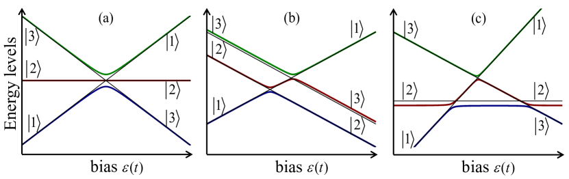
Figure 15: Three-level systems. Diabatic energy levels of states $\left|i\right\rangle$ (thin black lines) intersect in one (a), two (b), or three (c) points. Eigenenergies of the full Hamiltonian $H(t)$, as shown with thick color lines, exhibit avoided-level crossing. Note that in (c) there are two possible trajectories to get from $\left|1\right\rangle$ to the left into $\left|3\right\rangle$ to the right, which implies interference during the single-passage process.

Let us start here from the simplest realization of a multilevel system: the three-level one. If the system diabatic levels $\left|i\right\rangle$ depend linearly on the energy bias $\varepsilon(t)$ with possible offset between levels $h$, then the respective diabatic energy levels can be drawn as straight lines, as in Fig. 15, with one, two, or three intersections; here, $h=0$ is used for the case with a single intersection and $h\neq 0$ for the other cases. Taking into account possible tunneling, proportional to $\Delta$, lifts the degeneracies and results in avoided-level crossings. We can describe this with the Hamiltonian

$$H(t)=-\frac{\varepsilon(t)}{2}\widehat{A}-\frac{h}{2}\widehat{B}-\frac{\Delta}{2}\widehat{C},$$ (96)

with $\widehat{A}$, $\widehat{B}$, and $\widehat{C}$ being $3\times 3$ matrices; these can be expanded with Gell–Mann matrices Kiselev et al. (2013). Then, taking these matrices with the parameters, say, close to the ones of Ref. Ashhab (2016), we display in Fig. 15 several situations: (a) the “bow-tie” model, when all three levels (quasi-)intersect at one point, (b) the “equal-slope” model with the (avoided) crossing of the three levels in two points, and (c) the “triangle” model with three pairwise (quasi-) intersections. The most important aspect that distinguishes (c) from (a) and (b) is the possibility of interference during a single-passage dynamics. For example, there are two possible trajectories that lead from $\left|1\right\rangle$ to the left into $\left|3\right\rangle$ (or alternatively to $\left|2\right\rangle$) to the right in Fig. 15(c). This means that the final occupation probability is essentially defined by the phase difference between the two trajectories. Note that a three-level system can be described with a spin-1 Hamiltonian, so all theory for both single- and multiple-passage problems can be extended from two-level systems to three-level ones Zhang et al. (2011).

Let us now consider previous work done for driven multilevel systems, here separating the subject into three topics.

Theory

From the above example of a three-level system, we can formulate a generalized LZSM problem for a multilevel system, for example, as follows: what is the occupation probability of a state $\left|j\right\rangle$ if starting from a state $\left|i\right\rangle$? More generally, the evolution can be described by the matrix $S$ linking the final vector-state to an initial one Shytov (2004); Suzuki and Nakazato (2022). Here, as for the evolution of a TLS, it is instructive and most common to consider either a single-passage problem or periodic evolution with multiple passages. The “bow-tie” model describes a quasi-intersection of $N$ energy levels Ostrovsky and Nakamura (1997), while the “equal-slope” model is the (quasi-) intersection of the energy band, here with $N-1$ levels, by one more level Demkov and Osherov (1968). The single passage for a “bow-tie” and “equal-slope” models is described by sequential pairwise-level crossings Brundobler and Elser (1993). Magnetic sub-levels of two atomic levels with nonzero total angular momenta can be described by degenerate LZSM model, which involves two crossing sets of degenerate energy levels with quasi-crossing between them Vasilev et al. (2007).

As for a three-level case, for an $N$-level system, we can also have an extended “triangular” model, with several sequential crossings making trajectories meet Demkov and Ostrovsky (1995); Fai et al. (2015). In this case, even for a single-passage evolution, we can take possible interference into account Ostrovsky et al. (2007); Sinitsyn (2015); Malla et al. (2021).

The description of the $S$-matrix approach for single-passage problems is reviewed in Sinitsyn and Chernyak (2017). As an extension of this, we can interpret the method of solving rate equations, which we consider in a separate subsection. This method is applicable to periodically driven systems, as shown by Wen et al. (2010), for the example of multilevel devices based on superconducting circuits Berns et al. (2008); Oliver and Valenzuela (2009). Importantly, this latter approach takes a dissipative environment into account. An intuitive picture of open multilevel systems can be obtained by modeling the external environment by a harmonic oscillator Ashhab (2016). In the case of a weak interaction between $N$ spins-${\frac{1}{2}}$, the LZSM transitions can be described by a mean-field approach Garanin (2003).

Single passage in multilevel systems

Although a three-level system is useful as a prototypical model for introducing the features of multilevel systems, more realistic and widely used are those models with four levels. These describe coupled two-level systems or genuine four-level systems, such as double quantum dots with two electrons. The single passage problem with the four-level model was addressed, for instance, for two antiferromagnetically coupled tunneling systems, such as Mn₄ dimers Garanin (2004), Rydberg atoms Mallavarapu et al. (2021); Niranjan et al. (2020), and quantum dots Sinitsyn (2002); Reynoso and Flensberg (2012); Krzywda and Cywiński (2020). Not only qubits, but also qutrits, can be coupled, as in Refs. Grimaudo et al. (2019, 2020), which demonstrates that such coupling is useful for entanglement control.

Multiple-passage transitions in multilevel systems

Periodically driven three-level systems may describe a qubit coupled with two microscopic systems Sun et al. (2010) or a superconducting charge qubit that is taking a higher energy level into consideration Parafilo and Kiselev (2018a). A three-level model for a driven system is convenient for describing the impact of the external noise Kenmoe et al. (2013, 2015); Kenmoe and Fai (2016); Li and Cen (2018); Band and Avishai (2019). Periodically driven four-level systems are useful for describing the charge states of two particles in DQDs, as realized in Shi et al. (2014); Chatterjee et al. (2018); Mi et al. (2018) and described in Pasek et al. (2018); Shevchenko et al. (2018); Zhao and Hu (2022); Zhou et al. (2021). A five-level model describes singlet-triplet states in spin-based DQDs Stehlik et al. (2016b); Chen et al. (2017); Qi et al. (2017), which was also addressed by Zhao and Hu (2018a); Karami et al. (2019); Ginzel et al. (2020).

As a further development, triple quantum dots were also studied Aers et al. (2012); Poulin-Lamarre et al. (2015); Gallego-Marcos et al. (2016); Łuczak and Bułka (2016). These systems present more flexibility and controllability than DQDs while representing a minimal model for a chain of quantum dots, which can be considered a highly controllable quantum metamaterial Smirnov et al. (2007); Rakhmanov et al. (2008). The interference effects, here appearing in periodically driven coupled qubits, were extensively studied by Denisenko et al. (2010); Satanin et al. (2012); Gramajo et al. (2017, 2018, 2021); Munyaev and Bastrakova (2021).

V Quantum control

To summarize what we discussed above, LZSM transitions act as a tool to control a TLS’s occupation; that is, to control single-qubit states and the states of multi-level systems. As our system is analogous to a two-slit layout, a single-passage process presents a beam splitter for the energy-level occupation probabilities where the ratio of splitting can be controlled. Besides creating the coherent superposition, repeated passage of the avoided-level crossing gives the option to control the quantum system energy-level occupation probabilities by varying the accumulated dynamical phase.

Having obtained information about the quantum system, we can go further by studying opportunities for its control. In addition to other trends such as quantum simulations Georgescu et al. (2014); Buluta and Nori (2009) and quantum sensing Degen et al. (2017), coherent quantum control can be viewed as another direction in quantum engineering. Since it is important for applications to have individual control of single quantum systems, we will present here studies of LZSM non-adiabatic transitions and interference for the quantum control of few-level natural and artificial quantum systems.

V.1 Coherent control of microscopic and mesoscopic structures

The 2012 Nobel Prize in Physics was awarded for “experimental methods that enable measuring and manipulation of individual quantum systems”. To clarify, these systems were microscopic and consisted of atoms and photons. More recently, the variety of related quantum systems increased and also includes mesoscopic systems behaving as very large atoms Buluta et al. (2011). To demonstrate this, we present the following variety of systems and approaches where the underlying effective Hamiltonian can be readily modified or engineered and their coherent quantum control was studied in the frame of LZSM physics.

* In superconducting structures, the properties of non-adiabatic LZSM transitions can be used to control superposition states in single qubits Salmilehto and Möttönen (2011) and the entanglement in coupled-qubit systems Quintana et al. (2013). Several techniques were developed:

• amplitude spectroscopy Berns et al. (2008), which is applicable to multi-level systems, where increasing the driving amplitude results in reaching more avoided-level crossings for a single driving frequency that may be orders of magnitude smaller than the energy scales being probed;

• quantum phase tomography Rudner et al. (2008), which is based on the Fourier transforms of the interferograms that provide additional visibility and information;

• pulse imaging Bylander et al. (2009), where the measured interferograms are used to image the actual wave form of the driving signal at the device, which in turn can be used to engineer the desired time evolution of a quantum system. These and other similar methods provide means to characterize and manipulate states of superconducting and other quantum systems.

* Quantum dots, which can be charge or spin qubits, can be controlled. The hyperfine interactions can be harnessed for quantum control in GaAs semiconductor quantum dots Ribeiro et al. (2010). The visibility of quantum oscillations can be increased by enhancing the adiabatic passage probability. For this purpose the researchers designed tailored pulses that combined both fast and slow rise-time ramps to minimize dissipation and enhance adiabaticity Ribeiro et al. (2013a).

* A qubit can be coupled to a bath of TLSs describing noise in quantum circuits. Properly driving such TLSs can help to dynamically decouple such systems, thus reducing dielectric losses. This was demonstrated with TLSs in deposited aluminum oxide by using it as the dielectric in a lumped-element $LC$-resonator Matityahu et al. (2019). Using LZSM interference in quantum dynamics can help to isolate a single particle (in a quantum dot) from a Fermi sea by closing a tunnel barrier Kashcheyevs and Timoshenko (2012). The sensitivity of LZSM transitions to the parameters of the dissipative environment makes them useful for gauging a quantum heat bath Wubs et al. (2006). Using repetitive transitions with underlying interference allows accurately obtaining all relevant information about complex influences. This was observed in Ref. Forster et al. (2014) on the example of a two-electron charge qubit defined in a lateral double quantum dot.

* In composite or hybrid systems, non-adiabatic transitions can bring a system from one state to a desired state that might be entangled Li et al. (2011). For a system of qubits, the transfer state between qubits was studied with a photonic qubit (localized exciton in an optically active quantum dot) coupled to a spin qubit hosted in gate-defined quantum dots Joecker et al. (2019), with a composite system of Majorana-hosted semiconductor nanowire and superconducting flux qubits Zhang and Yu (2013), and with three superconducting qubits Li et al. (2019). For a hybrid system consisting of a qubit coupled to a photonic cavity, the transition results in the entanglement of the system and, the generation of Schrödinger cat states in the photonic cavity Lidal and Danon (2020).

* Adiabatic passages and nonadiabatic transitions in a macroscopic, cylindrically shaped water sample were studied using standard nuclear magnetic resonance (NMR) techniques with controlled linear ramping of the external magnetic field Hürlimann et al. (2020). The pulse sequence used in this experiment was the standard in NMR applications: the Carr-Purcell-Meiboom-Gill sequence.

* The similarity between driven TLS dynamics and other processes can provide a basis for simulating these phenomena with a highly controllable TLS. The emulation of mesoscopic phenomena, such as weak localization and universal conductance fluctuations, was demonstrated on a system of superconducting transmon qubits by Gramajo et al. (2020).

* Using the acquired phase of the wave function during single and repeated non-adiabatic transitions provides the basis for optimal control theory Zhdanov and Seideman (2015). Depending on the purpose (e.g., to obtain complete population transfer, which we will also address later), the driving signal can be tailored Larocca et al. (2018). The efficiency can be quantified with the methods of quantum metrology, and calculations of quantum Fisher information Yang et al. (2017).

* A driven TLS provides a testbed quantum thermodynamics Ono et al. (2020), where the non-adiabatic transitions serve to change states between different regimes. This was studied in Otto heat engines Halpern et al. (2019); Son et al. (2021), and in calorimetric methods and measurements of work Solinas et al. (2013); Pekola et al. (2013).

The following three subsections present specific chapters in the quantum control with LZSM transitions.

V.2 Universal single- and two-qubit control

Most often, quantum control (logic gates including) is associated with resonant driving that then results in Rabi oscillations Kwon et al. (2021); Krantz et al. (2019). However, under resonant driving, certain limitations may arise, including achievable gate speed and nonidealities, such as counter-rotating terms Vitanov et al. (2003); Saito et al. (2006); Longhi et al. (2019); Campbell et al. (2020). Coherent LZSM interference allows for a complementary approach to quantum control based on nonresonant driving with the alternation of adiabatic evolution and nonadiabatic transitions. This enables ultrafast qubit gates that are controlled solely using baseband pulses, hence alleviating the need for pulsed-microwave control signals Cao et al. (2013); Ota et al. (2018); Campbell et al. (2020); Zhang et al. (2021); Li et al. (2022).

Qubit evolution can be conveniently described by trajectories on the Bloch sphere. For this, the evolution matrices in the transfer matrix (TM) approach should be rewritten using the Euler-angle decomposition Sillanpää et al. (2006, 2007). First, to describe the nonadiabatic transition, we rewrite the $N$ matrix from Eq. (30) in the form

$$N=\left(\begin{array}[]{cc}\cos(\theta/2)e^{-i\phi_{\mathrm{S}}}&-\sin(\theta/2)\\ \sin(\theta/2)&\cos(\theta/2)e^{i\phi_{\mathrm{S}}}\end{array}\right)=U_{z}\left(\phi_{\mathrm{S}}\right)U_{x}\left(\theta\right)U_{z}\left(\phi_{\mathrm{S}}\right),$$ (97)

where $\sin^{2}(\theta/2)=\mathcal{P}$ and the matrices $U_{x,y,z}(\alpha)=\exp\left(-i\alpha\sigma_{x,y,z}/2\right)$ describe their respective rotations. The adiabatic evolution is characterized with the $z$-rotation $U(t,t_{\mathrm{i}})=\exp{(-i\zeta\sigma_{z})}$ in Eq. (27). Then, the single-passage evolution is described by $UN$, Eq. (34). The repetition of these can correspond to a one-period evolution (with doubly passing the avoided crossing), $\Xi=N^{\top}U_{2}NU_{1}$, Eq. (48), or to an $n$-cycle evolution with $\Xi^{n}$ in Eq. (53c). After writing this, we can equate the evolution matrix with the matrix for the Euler-angle decomposition $U(\alpha,\beta,\gamma)=U_{z}(\gamma)U_{y}(\beta)U_{x}(\alpha)$ Landau and Lifshitz (1965); as a result, we obtain the formulas for the designated rotation angles $\alpha$, $\beta$, $\gamma$. With this, we can obtain a desired protocol and the parameters for single-qubit operations Campbell et al. (2020). Here, the important claim is that with the pure LZSM interference technique, we can obtain any rotation and, correspondingly, the efficient single-qubit and two-qubit control Ribeiro et al. (2010). This approach allows for defining the parameters for a desired evolution or a unitary logic gate and for analyzing the resonance conditions Ashhab et al. (2007).

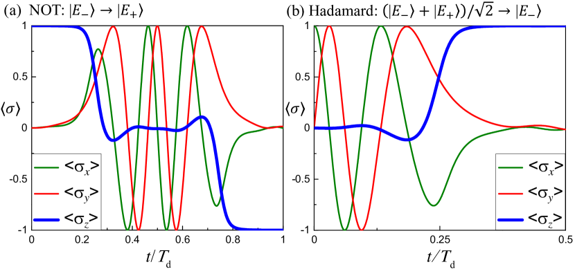
Figure 16: LZSM gates. Dynamics of $\sigma$-matrix coefficients $\left\langle\sigma_{x,y,z}\right\rangle$, which define the position on the Bloch sphere, under $\varepsilon(t)=A\cos\omega t$ driving. (a) NOT gate, which is the transfer $\left|E_{-}\right\rangle\rightarrow\left|E_{+}\right\rangle$, here as performed by two consecutive LZSM transitions. For this, we assume the constructive-resonance condition $\zeta+{\phi}_{S}=2\pi n$ (this defines the amplitude $A$) and take the transition probability $\mathcal{P}=0.5$. Specifically, we found $A=3.8872\Delta$ and the frequency was defined from $\omega=-\pi\Delta^{2}\left[2\hbar A\ln\mathcal{P}\right]^{-1}$. (b) Hadamard gate performed with the following parameters: $\mathcal{P}=0.5$, $A=4.309\Delta$, which is defined from the condition for destructive interference $\zeta+{\phi}_{S}=\frac{3\pi}{2}+2\pi n$.

As an illustrative example, consider first driving a TLS with pulses that result in a double passage of the avoided crossing Cao et al. (2013). This is described by the matrix $\Xi=N^{\top}U_{2}NU_{1}$, here with the alternation of adiabatic evolution ($z$-rotation) and nonadiabatic transition with the $N$ rotation matrix. We note that the rotation angles, both $\theta$ and ${\phi}_{\mathrm{S}}$, are defined by the adiabaticity parameter $\delta$ and, consequently, by the passage velocity $v$. Hence, adjusting the pulse shape (which defines this velocity $v$), one can obtain any rotation and respective logic gate Cao et al. (2013). For a fixed velocity, the evolution is limited between the two trajectories defined by destructive and constructive interference Ota et al. (2018).

In Fig. 16(a) we demonstrate the NOT operation, which is the rotation around the $x$ axis by the angle $\pi$. For this, we consider driving with a cosine pulse and choose the parameters to perform the NOT operation. Namely, we use $\mathcal{P}=0.5$ and the total phase changing during one LZSM transition ${\phi}_{\mathrm{S}}+\zeta=2\pi n$ to have the constructive interference, see Eqs. (28, 9). As a result, one can perform a fast and robust NOT operation, which in Fig. 16(a) illustrates the transition from the ground state (logical $0$) to the excited state (logical $1$): $\left|E_{-}\right\rangle\rightarrow\left|E_{+}\right\rangle$.

Next, consider the Hadamard gate. As above, this can be implemented with the double-passage process. However, with the chosen value $\mathcal{P}=0.5$, we can do this faster, here with a single-passage transition, which occurs during half the period. We illustrate this in Fig. 16(b). For performing the Hadamard gate, we use a single LZSM transition, with the total phase changing ${\phi}_{\mathrm{S}}+\zeta=3\pi/2+2\pi n$, resulting in $\left\{\left|E_{-}\right\rangle+\left|E_{+}\right\rangle\right\}/\sqrt{2}\rightarrow\left|E_{-}\right\rangle$. Hence, we have demonstrated two gates, and this can be supplemented by, for example, the phase gate to obtain the universal set of single-qubit operations. The phase gate can be realized by $U_{z}(\zeta)=\exp{(-i\zeta\sigma_{z})}$, which is idling (in the absence of driving).

In addition to single-qubit operations, two-qubit operations can also be done with LZSM transitions and interference. Two-qubit operations are conveniently demonstrated by the conditional phase gate or controlled-Z (CZ) gate between two qubits; four-level dynamics was studied by Rol et al. (2019); Campbell et al. (2020) for superconducting qubits and by Huang et al. (2018) for Rydberg atoms. Similarly, another two-qubit operation—the controlled-NOT (CNOT) operation—can be realized Ribeiro et al. (2010); Wu et al. (2021). Importantly, this approach allows for fast execution of the two-qubit operations with high fidelity. Provided one has single- and two-qubit operations, the next step could be the realization of algorithms.

Destructive interference can be harnessed to perform unitary transformations based on cyclic evolutions, which refer to the process where the state of the system returns to its original state after gate operations Wang et al. (2016). As a result of this evolution with destructive interference (i.e. coherent destruction of tunneling [CDT]), the state vector accumulates a phase only. This phase acquired in the evolution contains both dynamic and geometric components; see the detailed and pedagogical explanations in the supplementary material of Wang et al. (2016), and for relations to the Berry phase, see Lim et al. (2015a, b); Bleu et al. (2018). The geometric phase can be related to the solid angle subtended by the evolution curve on the Bloch sphere. This analysis opens up new ways of interpretation and control; this is called geometric LZSM interferometry Gasparinetti et al. (2011). Because we can perform any logic operations using this, it provides the instruments for geometric quantum computation. This is a promising approach to achieve robust control of a quantum system Tan et al. (2014); Zhuang et al. (2022); Barnes et al. (2022).

V.3 Shortcuts to adiabaticity

Two major aims of quantum control can be defined as either reaching a given target state or tracking the instantaneous ground state of a system during its evolution Bason et al. (2012). For each task, an optimum strategy can be designed based on requirements such as the highest possible fidelity, fastest possible operation, and so forth.

For illustration, the authors of Ref. Bason et al. (2012) considered both a shortcut protocol that reaches the maximum speed compatible with the Heisenberg uncertainty principle and the opposite limit of nearly perfectly following the instantaneous adiabatic ground state. For the LZSM-form Hamiltonian $H(t)=\left[-\Delta(t)\sigma_{x}-\varepsilon(t)\sigma_{z}\right]/2$, the authors designed a protocol that drives the system through avoided crossing in such a way that at the end of evolution, the final state $\left|\psi_{\mathrm{fin}}\right\rangle$ is as close as possible to the adiabatic ground state $\left|E_{-}(t_{\mathrm{fin}})\right\rangle$, which here aims to reach a unit’s final fidelity $\left|\left\langle\psi_{\mathrm{fin}}\right.\left|E_{-}(t_{\mathrm{fin}})\right\rangle\right|^{2}=1$. In general, there are infinitely numerous paths in Hilbert space connecting the initial state, for example, $\left|\psi_{\mathrm{ini}}\right\rangle=\left|E_{-}(t_{\mathrm{ini}})\right\rangle$ with the final one $\left|E_{-}(t_{\mathrm{fin}})\right\rangle$. First, fixing $\Delta(t)=\text{const}$, minimizing the evolution time results in a problem known as the shortcut to adiabaticity (STA) Guéry-Odelin et al. (2019); Chen et al. (2021b) or also by analogy with the equivalent classical case, “quantum brachistochrone” Oh et al. (2016). Here, the minimum time for reaching the target state is known as the quantum speed limit time:

$$T_{\mathrm{qsl}}=2\arccos\left|\left\langle\psi_{\mathrm{fin}}\right.\left|\psi_{\mathrm{ini}}\right\rangle\right|/\Delta.$$ (98)

In the opposite formulation, aiming at perfect following the ground state $\left|E_{-}(t)\right\rangle$ is known as the counterdiabatic protocol Demirplak and Rice (2003) or superadiabatic protocol Berry (2009). Details of this transitionless adiabatic protocol are considered below.

As mentioned, there are two major routes for manipulating the state of a quantum system with interacting fields: either using resonant pulses or adiabatic methods Chen et al. (2010). The most popular methods for efficient population transfer are the adiabatic rapid passage (ARP; sometimes RAP), chirped-pulse excitation or Stark-chirped RAP (SCRAP), and stimulated Raman adiabatic passage (STIRAP) Vitanov et al. (2001); Goswami (2003); Wei et al. (2008). The latter technique permits the precise control of population transfer using partially overlapping pulses, from pump and Stokes lasers Bergmann et al. (1998). In its simplest form, for a three-level system, the pump pulse links the initial state $\left|1\right\rangle$ with an intermediate state $\left|2\right\rangle$, which, in turn, interacts via a Stokes (or dump) pulse with a target state $\left|3\right\rangle$; the aim of this pump–dump technique is to achieve complete transfer of a population between states $\left|1\right\rangle$ and $\left|3\right\rangle$.

The STIRAP technique can be interpreted as pairs of LZSM transitions in the areas of avoided crossings of quasienergies Yatsenko et al. (1998); Malinovsky and Krause (2001). If the avoided crossing is passed repeatedly, the interference has to be taken into account Vitanov (2018). This was also analyzed by Zhang and Liu (2019), in which the nonadiabatic transitions were quantified by the upper-bound function, hence providing the optimal criteria for adiabatic control. In relation to our previous discussion on the interrelation between LZSM interference and multi-photon processes, coherent population transfer can also be described as multi-photon ARP Maeda et al. (2006). The ARP strategy can be used for a high-quality source of single photons that are emitted because of spontaneous emission from the excited state, which is robust against control errors and environmental fluctuations Miao and Zheng (2016b).

To understand the idea of counter-diabatic driving, consider this, following Demirplak and Rice (2003) and Theisen et al. (2017): let our arbitrary $n$-level system be described by the Hamiltonian $H(t)$, and let $U(t)$ be a time-dependent unitary transformation that makes the matrix $U(t)H(t)U^{{\dagger}}(t)$ diagonal; it consists of the eigenvectors of $H(t)$. Consider now the full Hamiltonian $\widetilde{H}(t)=H(t)+H_{\mathrm{CD}}(t)$. Then, retaining the definition of $U(t)$, consider the new Hamiltonian after such transformation

$$\widetilde{H}^{\prime}=U\widetilde{H}U^{{\dagger}}-i\hbar U\dot{U}^{{\dagger}}=UHU^{{\dagger}}+\left(UH_{\mathrm{CD}}U^{{\dagger}}-i\hbar U\dot{U}^{{\dagger}}\right).$$ (99)

Because a priori, $UHU^{{\dagger}}$ is diagonal, then the condition

$$H_{\mathrm{CD}}=i\hbar\dot{U}^{{\dagger}}U$$ (100)

guarantees that at all times, the population, which was placed initially in one of the adiabatic states, remains exactly in that particular state.

Alternatively, the counter-diabatic Hamiltonian $H_{\mathrm{CD}}(t)$ can be written following Berry (2009) in terms of the instantaneous eigenvalues $E_{n}(t)$ and eigenstates $\left|\psi_{n}(t)\right\rangle$ of the system Hamiltonian $H(t)$

$$H_{\mathrm{CD}}=i\hbar\sum_{m\neq n}\sum_{n}\frac{\left|\psi_{m}\right\rangle\left\langle\psi_{m}\right|\dot{H}\left|\psi_{n}\right\rangle\left\langle\psi_{n}\right|}{E_{n}-E_{m}}.$$ (101)

Consider this for a TLS with a generic Hamiltonian $H(t)=-\left[\Delta(t)\sigma_{x}+\varepsilon(t)\sigma_{z}\right]/2$. This is written in the diabatic (time-independent) basis $\left\{\left|0\right\rangle,\left|1\right\rangle\right\}$, and the transformation to the instantaneous basis $\left\{\left|E_{-}(t)\right\rangle,\left|E_{+}(t)\right\rangle\right\}$ is defined by the angle $\theta(t)=\,$$\arctan\frac{\Delta(t)}{\varepsilon(t)}$. Then, Eq. (101) gives

$$H_{\mathrm{CD}}(t)=\frac{\hbar}{2}\dot{\theta}(t)\sigma_{y}.$$ (102)

We emphasize that this formula is valid for any $\Delta(t)$ and $\varepsilon(t)$, leaving the system in an eigenstate of $H(t)$. In particular, for the linear LZSM problem, with $\dot{\Delta}=0$ and $\dot{\varepsilon}=v$, we obtain

$$\widetilde{H}(t)=-\frac{\Delta}{2}\sigma_{x}-\frac{vt}{2}\sigma_{z}+\frac{v\Delta}{\Delta^{2}+v^{2}t^{2}}\sigma_{y}.$$ (103)

Note that the time integration of $\dot{\theta}(t),$ from $-\infty$ to $\infty,$ gives $\pi$ so that $\dot{\theta}(t)$ represents a $\pi$-pulse Theisen et al. (2017). More generally, for pulse areas equal to odd multiples of $\pi$, a complete population transfer to the excited state takes place, whereas for pulse areas equal to even multiples of $\pi$, the system returns to the initial state Vitanov et al. (2001); Teranishi and Nakamura (1999).

Therefore, for a perfect adiabatic behavior, the nonadiabatic transitions should be suppressed, for which the LZSM model is central for testing control protocol. This was discussed for TLSs Chen et al. (2010); Ahmadinouri et al. (2019); Funo et al. (2021), for three-level systems Theisen et al. (2017), and for $n$-level ones Poggi et al. (2015); Xu et al. (2018). In particular, it is possible to approximately decompose the transitionless quantum driving into the sum of separate single-crossing corrections Theisen et al. (2017). Analysis of the adiabatic condition can help further improve the coherent population transfer, resulting in tangent-shaped pulses Xu et al. (2019a).

In some cases, it is possible to reach diabaticity by excluding the $\sigma_{y}$ component by certain system-specific transformation Bason et al. (2012) or by applying additional fast and strong oscillating terms to a linear one, as in $\varepsilon(t)$ Chasseur et al. (2015). Indeed, as it was scrutinized by Petiziol et al. (2018), adding a fast oscillation in the control parameters can approximately (to arbitrary precision) cancel nonadiabatic effects. Hence, with this, transitionless dynamics can be realized for finite-dimensional quantum systems without requiring additional Hamiltonian components that are not included in the initial control setup; this was further developed for single and coupled qubits (creating entanglement between them), as well as for three-level systems Petiziol et al. (2018); Petiziol and Wimberger (2019); Petiziol et al. (2019).

The techniques of population transfer that we considered here were tested and developed for diverse physical realizations: atoms and molecules controlled by lasers Vitanov et al. (2001), Bose–Einstein condensate Bason et al. (2012), Rydberg states Shi et al. (2016); Bengs et al. (2022), photonic structures Longhi (2009) (see therein for classical analogies), NMR Herrera et al. (2014), electron spin of a single NV center in diamond Zhang et al. (2013), electron spin in a QD Shafiei et al. (2013) (see for chirping back and forth resulting in a double-passage dynamics; for theory see Teranishi and Nakamura (1999); Nagaya et al. (2002)), ensemble of QDs to demonstrate an ideal molecular switch with the LZSM formalism Kaldewey et al. (2018), superconducting qubits Wei et al. (2008), and topologically protected edge states in a dimeric spin chain Longhi et al. (2019).

V.4 Adiabatic quantum computation

Adiabatic quantum computation (AQC) is an approach to quantum computing that is an important alternative to the standard circuit (gate) model. In principle AQC is expected to be as powerful as the circuit model of quantum computation Albash and Lidar (2018); Ashhab et al. (2006). The former is not very sensitive to dephasing, yet the huge cost of this approach is the lack of universality and problems with accurate calculations Zagoskin (2011). AQC is best suited for optimization problems, where the requirement is to find the global minimum of a cost function. In AQC, the computation proceeds from a simple initial Hamiltonian $H_{\mathrm{i}}$, whose ground state is easy to prepare, to a final Hamiltonian $H_{\mathrm{f}}$, whose ground state encodes the solution to the computational problem. Hence, the task is to find the ground state of $H_{\mathrm{f}}$, whose unknown eigenvalues determine the cost function. The evolution is described by the Hamiltonian

$$H(s)=(1-s)H_{\mathrm{i}}+sH_{\mathrm{f}},$$ (104)

so that at $t=0$ with $s=0$, we start from $H_{\mathrm{i}}$, and at the end of computation at $t=t_{\mathrm{f}}$ with $s=1$, we have the desired final Hamiltonian $H_{\mathrm{f}}$ Cullimore et al. (2012). The eigenvalues and eigenstates of the Hamiltonian $H(s)$ describing a system of $M$ qubits are given by $H(s)\left|\varphi_{m}(s)\right\rangle=E_{m}(s)\left|\varphi_{m}(s)\right\rangle$, with $m$ ranging from $0$ to $2^{M}-1$. The suitable figure of merit is the closeness of the state vector $\left|\psi(s)\right\rangle$ at the end of the evolution to the desired state $\left|\varphi_{0}(s)\right\rangle$. This is quantified by the success probability $\left|\left\langle\varphi_{0}(1)\!\right.\left|\psi(1)\right\rangle\right|^{2}$.

For adiabatic evolution, the cornerstone of this is the adiabatic theorem, which assumes no LZSM transitions Johansson et al. (2009). The avoided crossings are defined by the minima of $\Delta E(s)=E_{1}(s)-E_{0}(s)$. Hence, in the vicinity of these minima, the low-energy Hamiltonian is equivalent to the one describing two wells that are connected by a tunneling rate and detuned from each other by a bias Wild et al. (2016). In this case, LZSM transitions are usually considered a nuisance for AQC Grajcar et al. (2005). Also, LZSM theory tells us that, akin to a double-slit experiment, two consecutive transitions (at the minima of $\Delta E(s)$) can generate interference effects Lubin et al. (1990); Munoz-Bauza et al. (2019).

Therefore, studying LZSM physics in an open system with the Hamiltonian $H(s)$ can help minimize undesired nonadiabatic transitions Wild et al. (2016). Because, on the one hand, the system has to evolve adiabatically slow to avoid nonadiabatic transitions and, on the other hand, we want to make the calculations faster, there are several ways to satisfy these two conflicting requirements. For this, we must make the control of the feedback in calculations, monitoring the curvature of the ground state $E_{0}(s)$. Then, the feedback-control scheme speeds up the computation process by allowing for faster evolution of $s(t)$ when the ground state is well separated from the excited one Wilson et al. (2012). Alternatively, the success probability can be increased by tailoring the driving pulses Karanikolas and Kawabata (2020). These quantum annealing protocols, called pulsed quantum annealing, are reached by optimizing the pulse parameters. Also, in the context of AQC, an additional periodic drive can be applied to suppress control errors by using a destructive LZSM interference, which is known as coherent destruction of tunneling (CDT) Atia et al. (2019).

Because the minimal gap between the ground and first excited state can decrease with an increasing number of qubits $M$, in general, the probabilities of nonadiabatic transitions are nonzero and should be taken into account Santoro (2002). Then, the question arises regarding how far the evolution can deviate from the ground state and still obtain useful results. Taking these into account results in the approximate AQC. Particularly, estimating the efficiency in this case, here for a large number of possible interlevel transitions, can be done by using the analogy of the evolution with the standard random walk Zagoskin (2011). Indeed, let us denote by $N\gg 1$ the average number of avoided-level crossings per one energy level, $\kappa=sN$ an estimate number of avoided-level crossings, $q=q(n,\kappa)$ the probability of finding the system in the eigenstate $\left|\varphi_{n}(s)\right\rangle$, and $p$ the average LZSM transition probability. Then, assuming $n\gg 1$, after passing an avoided-level crossing, the system can be found in the $n$-th state if either it stays in this state or if it underwent a nonadiabatic transition from a neighboring energy level:

$$q(n,\kappa+1)=(1-p)q(n,\kappa)+\frac{p}{2}\left[q(n-1,\kappa)+q(n+1,\kappa)\right]\text{.}$$ (105)

This is almost the equation for the standard random walk Zagoskin (2011), which allows us to use standard methods to describe the statistics of multiple LZSM transitions in a multilevel system. For instance, the final dispersion reads

$$\left\langle\left(n-n_{0}\right)^{2}\right\rangle_{s=1}=pN,$$ (106)

which is proportional to the average transition probability $p$ and the average number of quasicrossings $N$. Furthermore, we note that for a linear bias, $s=t/t_{\mathrm{f}}$, the driving velocity $v$ is inversely proportional to the evolution duration $t_{\mathrm{f}}$. Then, the LZSM probability gives an estimation for the accuracy of the approximate AQC:

$$\sqrt{\left\langle\Delta n^{2}\right\rangle}\propto\exp\left(-\alpha t_{\mathrm{f}}\right),$$ (107)

which is defined by the exponential dependence on $t_{\mathrm{f}}$ with some nonuniversal rate $\alpha$.

VI Related classical coherent phenomena

On many occasions, the similarities between classical wave optics and quantum wave mechanics have been highlighted Dragoman (2004); Longhi (2009); Bondar et al. (2013); Bliokh et al. (2013); Dressel et al. (2014). In particular, in our context, we can find numerous examples in the literature where nonadiabatic transitions between classical states have been interrelated with LZSM physics. Some examples that can be mapped to the precession of a spin-1/2 particle exhibiting LZSM-type nonadiabatic transitions between two states, modes, and so forth, include the following: transformation of electromagnetic waves Zheleznyakov et al. (1983); Bliokh and Grinyok (2001), topological boundary states in acoustic waveguides Chen et al. (2021a, c), two coupled photonic crystal nanocavities (forming a photonic molecule) that are tuned by RF surface acoustic waves Kapfinger et al. (2015); Bliokh and Nori (2019), magnetoresistance in quasi-one-dimensional organic conductors Cooper and Yakovenko (2006), the mixing of two tones in a ferrimagnetic sphere resonator Mathai et al. (2020), optical modes coupled by a moveable membrane in optomechanical systems Wu et al. (2013); Jiang et al. (2020), two modes of a mechanical resonator or two directly-coupled resonators Zhang et al. (2020), and a rolling sphere on a Cornu spiral Rojo and Bloch (2010). In these systems, different realizations of classical analogues of Rabi oscillations and LZSM transitions and interference were demonstrated.

To be specific, in this section, we demonstrate that a system of two weakly coupled resonators can be described analogously to a quantum TLS. Namely, we demonstrate that under appropriate conditions, the Newton equations for this classical system are reduced to an equation formally analogous to the Schrödinger equation for a TLS. As a consequence, the classical system can display a classical analogue of LZSM transitions and interference. In addition, any physical system that can be mapped on a two-resonator system with weak coupling could behave similarly. In Fig. 17, we demonstrate a variety of such systems Ivakhnenko et al. (2018).

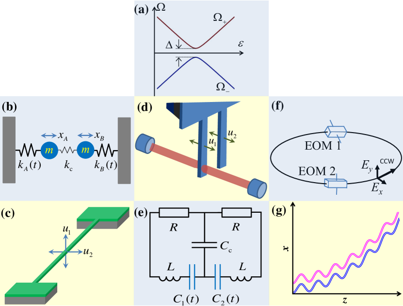
Figure 17: Different classical systems that behave analogously to quantum TLSs. In (a) the two eigenfrequencies, $\Omega_{\pm}$ are shown to depend on the bias $\varepsilon$ and display avoided-level crossing at $\varepsilon=0$ with a minimal distance $\Delta$. (b-g) Several possible classical systems that have eigenfrequencies as in (a). Namely, (b) two weakly coupled spring oscillators Frimmer and Novotny (2014), (c) two-mode nano-beam Faust et al. (2012); Seitner et al. (2016), (d) optomechanical system with two cantilevers, one of which is coupled with an optical cavity Fu et al. (2016, 2018), (e) two coupled electrical resonators Alzar et al. (2002); Muirhead et al. (2016), (f) two polarization modes of light propagating in the counter-clockwise (ccw) direction tuned by the electro-optic modulators, EOM1 and EOM2, with the tuning parameter being the electric field inside EOM1 Spreeuw et al. (1990); Beijersbergen et al. (1992), and (g) two coupled curved waveguides in which an electromagnetic wave is spread between them Longhi (2009); Liu et al. (2019).

From Newton to Schrödinger

We now consider how the classical Newton equations for two coupled resonators can be mapped to the Schrödinger equation for a quantum TLS. Here, we follow Refs. Novotny (2010); Frimmer and Novotny (2014). Consider the system of classical Newton equations for two weakly coupled oscillators $A$ and $B$, Fig. 17(b),

$$\begin{cases}m_{A}\ddot{x}_{A}+\gamma_{A}\dot{x}_{A}+k_{A}x_{A}+k_{c}\left(x_{A}-x_{B}\right)=0,\\ m_{B}\ddot{x}_{B}+\gamma_{B}\dot{x}_{B}+k_{B}x_{B}+k_{c}\left(x_{A}-x_{B}\right)=0,\end{cases}$$ (108)

where $x_{A,B}$ are the coordinates, $m_{A}=m_{B}=m$ are the masses, $\gamma_{A}=\gamma_{B}=\gamma$ are the damping coefficients, $k_{A,B}$ are the spring coefficients, and $k_{c}$ is a coupling coefficient that is assumed to be weak, $k_{c}\ll k_{A,B}$. To obtain an analogy with a quantum TLS, we choose the excitation in the form $k_{A,B}=k_{0}\pm\Delta k(t)$ with $\Delta k\ll k_{0}$. We denote the interaction-shifted eigenfrequency $\Omega_{0}^{2}\equiv(k_{0}+k_{c})/m$, and rewrite this system of classical Newton equations in matrix form, here using Pauli matrices:

$$\left(\frac{d^{2}}{dt^{2}}+\frac{\gamma}{m}\frac{d}{dt}+\Omega_{0}^{2}\right)\begin{bmatrix}x_{A}\\ x_{B}\end{bmatrix}-\left(\frac{k_{c}}{m}\sigma_{x}+\frac{\Delta k(t)}{m}\sigma_{z}\right)\begin{bmatrix}x_{A}\\ x_{B}\end{bmatrix}=0.$$ (109)

We use the ansatz

$$\frac{\tilde{x}_{A,B}(t)}{x_{0}}=\psi_{A,B}\exp{\left(i\Omega_{0}t\right)},~{}~{}~{}~{}~{}~{}x_{A,B}=x_{0}\text{Re}~{}\tilde{x}_{A,B}.$$ (110)

Here, $x_{0}$ is the initial deviation of the springs, which is used to normalize $\tilde{x}_{A,B}$. We obtain the equation

$$\left(\frac{d^{2}}{dt^{2}}+\left(\gamma+2i\Omega_{0}\right)\frac{d}{dt}+i\Omega_{0}\gamma\right)\begin{pmatrix}\psi_{A}\\ \psi_{B}\end{pmatrix}-\left(\frac{k_{c}}{m}\sigma_{x}+\frac{\Delta k(t)}{m}\sigma_{z}\right)\begin{pmatrix}\psi_{A}\\ \psi_{B}\end{pmatrix}=0.$$ (111)

We can simplify this equation by using two assumptions

$$\gamma\ll\Omega_{0}\text{ \ and \ }k_{c},\text{ }\Delta k\ll k_{0}.$$ (112)

The former assumption of small dissipation allows for neglecting $\gamma$ in comparison with $\Omega_{0}$. The latter assumption, together with the ansatz (110), allows to use the slowly varying envelope approximation, which consists of neglecting the second derivative. This means that $\psi_{A,B}$ have small changes during the time span $2\pi/\Omega_{0}$; in other words, the characteristic evolution rate for $\psi_{A,B}$ is much smaller than $\Omega_{0}$. Also, the assumption $\Delta k\ll k_{0}$ means that we cannot reach a fast transition, where $v\rightarrow\infty$ and $\left|\psi_{A}^{2}(t)\right|\rightarrow\theta(t)\mathcal{P}$. After using these assumptions, we obtain a Schrödinger-like equation

$$\color[rgb]{1,.5,0}\boxed{\color[rgb]{0,0,0}i\frac{d}{dt}\left|\psi\right\rangle=H(t)\left|\psi\right\rangle-i\frac{\gamma}{2}\left|\psi\right\rangle,\color[rgb]{1,.5,0}}\color[rgb]{0,0,0}$$ (113)

where $\left|\psi\right\rangle=\left(\psi_{A},\psi_{B}\right)^{\top}$and $H(t)$ is the Hamiltonian of Eq. (1) with

$$\Delta=\frac{k_{c}}{m\Omega_{0}}\approx\frac{k_{c}}{\sqrt{mk_{0}}},\text{ \ \ }\>\>\>\>\>\varepsilon(t)=\frac{\Delta k(t)}{m\Omega_{0}}\approx\frac{\Delta k(t)}{\sqrt{mk_{0}}}.$$ (114)

Much like qubits, the mechanical resonators can be driven via $\Delta k(t)$, to have both an offset and a periodic excitation, we have $\varepsilon(t)=\varepsilon_{0}+A\cos\omega t$. Note that the problem of Eq. (113) can be described in terms of a non-Hermitian Hamiltonian Shen et al. (2019).

In the absence of dissipation, $\gamma=0$, Eq. (113) formally coincides with the Schrödinger equation for a TLS, Eq. (15), in the natural measuring system, that is, assuming $\hbar=1$. Dissipation can be eliminated by the substitution $\left|\psi\right\rangle=\left|\overline{\psi}\right\rangle\exp{\left(-\gamma t/2\right)}$; then, the classical Schrödinger-like equation (113) becomes $i\frac{d}{dt}\left|\overline{\psi}\right\rangle=H(t)\left|\overline{\psi}\right\rangle$. In addition, the “density matrix” can be introduced as $\rho=\left|\psi\right\rangle\left\langle\psi\right|$, where $\left\langle\psi\right|:=\left(\psi_{A}^{\ast},\psi_{B}^{\ast}\right)$. Then, for the derivative, we obtain

$$\dot{\rho}=-i\left[H,\rho\right]-\gamma\rho.$$ (115)

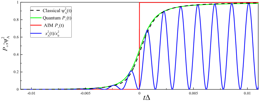
Figure 18: Single-passage transition in classical and quantum cases. We here compare the solutions of the classical Newton equations, Eq. (109), the Schrödinger equation, and Eq. (15) for a LZSM transition. For illustration purposes, we take the parameters so that the final excitation probability is close to unity, $\mathcal{P}\approx 1$. The classical transfer of energy from one harmonics to another is given by the black line $\left|\psi_{A}^{2}(t)\right|$, which virtually coincides with the quantum upper-level occupation probability $P_{+}(t)$, which is the green line. Furthermore, the red curve shows the AIM, which is considered above and is given here by $\theta(t)\mathcal{P}$; the blue curve shows the classical oscillations $x_{A}^{2}(t)/x_{0}^{2}$.

This coincides with the Bloch equation for a TLS, Eq. (87), for the Hamiltonian $H(t)$, and assuming that $\hbar=1$ and with equal relaxation rates, $T_{1}=T_{2}=1/\gamma$.

This means that we can use the same methods for solving the classical and quantum systems. Interestingly, historically, the system of nonadiabatic transitions between two states was first studied and developed for a quantum TLS, and only later it was recognized that it has a classical doppelgänger. Particularly, the theory by Zener helped describe the coupled pendulums in Ref. Maris and Xiong (1988).

In a system of two coupled classical oscillators, two eigenfrequencies are analogous to the two energy levels for the quantum TLS; these are the eigenvalues of the Hamiltonian above

$$\Omega_{\pm}=\pm\sqrt{\Delta^{2}+\varepsilon_{0}^{2}}.$$ (116)

The probability of the occupation of the energy levels in the quantum TLS is analogous to the squared amplitude of the oscillations $\left|\psi_{A,B}\right|^{2}$; in other words, it is proportional to the amount of energy in that oscillation mode. To further demonstrate the similarity of the classical problem to its quantum analogue, in Fig. 18, we consider a single-passage LZSM-like transition with $\varepsilon(t)=vt,$ and choose the following parameters: $\Delta_{c}/k_{0}=5\times 10^{-4}$ for the classical case and $\delta=\delta_{cl}\equiv k_{c}^{2}/4v=3.57\times 10^{-4}$ for both cases. This demonstrates that under the conditions (112), the classical envelope $\left|\psi_{A}(t)\right|^{2}$ corresponds to the quantum occupation probability $P_{+}(t)$. This principle can be applied for any classical system of two coupled resonators with weak coupling.

Coherent phenomena in classical mechanical systems were reliably demonstrated experimentally; see the caption of Fig. 17. In particular, LZSM interferometry was realized with mechanical resonators in Refs. Seitner et al. (2017) and Zhou et al. (2019); Lorenz et al. (2022). For further theoretical study of such processes, see Refs. Chotorlishvili et al. (2011); Parafilo et al. (2012); Parafilo and Kiselev (2018b); Villazon et al. (2019).

Engineered photonic waveguides

Curved waveguides have recently provided a rich laboratory tool to visualize quantum coherent phenomena with classical optical waves in the spatial domain Longhi (2009); Menchon-Enrich et al. (2016). To understand how this becomes possible, consider the propagation of monochromatic light waves of wavelength $\lambda$ along a curved waveguide structure. This could be a single waveguide, coupled ones, or multiple waveguides Longhi (2009); Morales-Molina and Reyes (2011); Reyes et al. (2012); Liu et al. (2019). Let the waveguide structure be planar, in the plane $\left(x,z\right)$; see Fig. 17(g). There, $z$ is the paraxial propagation distance, the axis bending profile $n_{s}$, and the refractive index profile of the guiding structure $n(x)$, $\omega=kc_{0}$. Using the scalar and paraxial approximations, we can write the electric field amplitude as $\psi(x,z)\exp\left[i\left(kn_{s}z-\omega t\right)+c.c.\right]$, where the slow-varying field envelope $\psi$ is described by the paraxial wave equation

$$i\lambdabar\frac{\partial\psi}{\partial z}=-\frac{\lambdabar^{2}}{2n_{s}}\frac{\partial^{2}\psi}{\partial x^{2}}+U(x)\psi,$$ (117)

with $\lambdabar=\lambda/2\pi$ and $U(x)=\left[n_{s}^{2}-n^{2}(x)\right]/2n_{s}\simeq n_{s}-n(x)$. This equation, Eq. (117), can be formally written in the form of a 1D Schrödinger equation with the following substitutions: $\lambdabar\rightarrow\hbar$, $n_{s}\rightarrow m$, and $z\rightarrow t$. Furthermore, the eigenmodes of two coupled waveguides can be described by a Hamiltonian formally analogous to the one of a driven TLS Liu et al. (2019).

To conclude, electromagnetic waves propagating along waveguides have different advantages, such as long coherent lengths and high control in preparation and measurement in a room-temperature environment. Given that the Maxwell equation for these takes the form of the Schrödinger equation and the interwaveguide interactions are analogous to the interaction between the quantum states, the light propagating along curved waveguides (namely, its intensity distributions) in the spatial domain can simulate quantum driven dynamics in the time domain Longhi (2009); Liu et al. (2019); Shen et al. (2019).

VII Conclusion

An avoided-level crossing is described by the LZSM model, which includes adiabatic evolution, nonadiabatic transitions, and quantum interference. We considered this by starting from the original LZSM works. It was demonstrated that this evergreen problem provides important tools for characterizing and controlling quantum systems.

Our detailed consideration of the works by Landau, Zener, Stückelberg, and Majorana demonstrates that the nonadiabatic transitions should be attributed to all four names. When presenting these four approaches here, we wanted not only to attract researchers’ attention to this, but to make these diverse approaches easily accessible and clear for modern readers. We focused on Zener’s approach because this describes both the final wave function, including its phase, and the dynamics. Both Zener’s and Majorana’s approaches can be developed to describe a few or many times passing of avoided-level crossing, providing the basis for the AIM in terms of transfer matrices.

In describing single- and multiple-passage problems, we supplemented previous works and the review Shevchenko et al. (2010). In that review, besides theory, mainly experiments with superconducting quantum systems were described. Here, we presented many more works, particularly the ones that have appeared since then, including on semiconducting devices, graphene, ultracold gases, and many other systems.

Single and multiple LZSM transitions display rich physics of quantum systems, both on microscopic and mesoscopic scales. Related physics can be harnessed to characterize their quantum dynamics (interferometry) and to control their states. Classical systems can also display analogous phenomena.

Appendix A LZSM transition probability

Here we present four ways to derive the LZSM formula, Eq. (7), following the four classic papers from 1932. In our presentation we follow the original works and make those derivations clear for a broad audience. For this sake, some derivations are simplified and some notations changed. Readers interested in the original works can find them in Refs. Landau (1932a, b); Zener (1932); Stückelberg (1932); Majorana (1932) and translated into English in Refs. Haar (1965); Cifarelli (2020a); Stueckelberg (1970). Presenting these together, allows to see the interrelation between these approaches. For example, C. Zener and E. Majorana solved the very same second-order differential equation, both by referring to the same book “Modern Analysis” Whittaker and Watson (1920), but Zener made use of special functions, while Majorana used the Laplace transform. Also, while following the LZSM papers, we will make several remarks; for example, we will not only be interested in the upper-level excitation probability, but also in the changes of the wave function phase, which is important for quantum-mechanical interference.

A.1 Near-adiabatic limit (Landau)

First, we consider the LZSM transition following L.D. Landau’s two original papers Landau (1932a, b), which have been translated into English in Haar (1965), and the textbook Landau and Lifshitz (1965). This derivation of the LZSM formula is arguably the simplest one.

Consider a slowly varying (with $v\ll\Delta^{2}/\hbar$) time-dependent Hamiltonian (1). To describe the adiabatically slow variations, one can consider time $t$ as a parameter, and the system dynamics described by the Schrödinger equation

$$H(t)\left|\psi(t)\right\rangle=E\left|\psi(t)\right\rangle.$$ (118)

We substitute the wave function (3) in the Schrödinger equation  (118) and obtain

$$(H-E)\begin{pmatrix}\alpha\\ \beta\end{pmatrix}=-\frac{1}{2}\begin{pmatrix}\ vt+2E&\ \Delta\\ \Delta&\ -vt+2E\end{pmatrix}\begin{pmatrix}\alpha\\ \beta\end{pmatrix}=0.$$ (119)

For a nontrivial solution of this matrix system of equations, we need to equate the matrix determinant to zero. As a result, we obtain the two energy levels of this TLS

$$E_{\pm}(t)=\pm\frac{1}{2}\sqrt{\Delta^{2}+\varepsilon(t)^{2}}=\pm\frac{1}{2}\sqrt{\Delta^{2}+(vt)^{2}}\equiv\pm\frac{\Delta E(t)}{2}.$$ (120)

For slow excitations ($v\ll\Delta^{2}/\hbar$), it is assumed that the evolution is adiabatic everywhere except for the avoided-crossing region. Then, we determine the probability of the upper-energy-level occupation $P_{+}(t\rightarrow+\infty)$, provided that the system was initially in its ground state $\left|0\right\rangle$, which means $P_{-}(t\rightarrow-\infty)=1$.

Slow perturbation implies that at large times of the “transition process”  the change of the action $S=\int E(t)dt$ is large. This means that the dynamics has a quasi-classical character and it is fully analogous to the over-barrier reflection. Note that we have the quasiclassical wave function as a function of time, not versus coordinates. Therefore, the avoided-crossing region determines the transition probability between the energy levels. In this region, the energy levels do not have an intersection in real space, but they have an intersection in complex space, so the equation $E_{+}(t_{0})=E_{-}(t_{0})$ is fulfilled at $t_{0}=\pm i\Delta/v$. Therefore, we can obtain the probability of the transition by following section 53 in Ref. Landau and Lifshitz (1965):

$$P_{+}=\exp{\left(-\frac{2}{\hbar}\mathrm{Im}\int_{0}^{t_{0}}[E_{+}(t)-E_{-}(t)]dt\right).}$$ (121)

Using the substitution $u=vt/\Delta$, we obtain the integral

$$\int_{0}^{t_{0}}\Delta E(t)\;dt=\frac{\Delta^{2}}{v}\int_{0}^{i}\sqrt{1+u^{2}}\;du=i\frac{\pi\Delta^{2}}{4v}.$$ (122)

Therefore, we obtain the excitation probability of the TLS for the linear perturbation, $P_{+}=\mathcal{P}=\exp{(-2\pi\delta)}$, which is Eq. (7).

In fact, in the original paper Landau (1932b), in the right-hand side of the formula (121), there should be a prefactor $C\sim 1$. This happened to be exactly unity for the LZSM formula, as we can see from each of the three following subsections.

The formula (121) is very convenient for calculating the single-transition probability for any bias signal, and we consider this in the main text for a nonlinear drive. Because the approach by Landau was generalized in Refs. Dykhne (1962); Davis and Pechukas (1976) for calculating nonadiabatic transitions regarding the form of the Hamiltonian, this formula is sometimes referred to as a Landau-Dykhne or Dykhne-Davis-Pechukas formula Vitanov and Suominen (1999); Lehto and Suominen (2015). Particularly, see the latter references for a generalization to the case when there are multiple zero points.

A.2 Using parabolic cylinder functions (Zener)

In this section, we consider how to derive the probability of the LZSM transition by following the work by Clarence Zener, Ref. Zener (1932). In fact we develop Zener’s approach by finding analytically the full wave function with the time dependence Vitanov and Garraway (1996); Shevchenko et al. (2010). Here we pay more attention to find the wave function’s phase change after the transition. In this approach, we obtain a straightforward solution of the Schrödinger equation with time dependence in terms of a special function, known as the parabolic cylinder function. This method is not so simple as the previous one, but it provides a more general and precise solution of this problem. In particular, there will be no unknown prefactor $C$, as in the approach by Landau. For a theoretical description involving a generalization for non-Hermitian Hamiltonians, see Shen et al. (2019); Kam and Chen (2021).

Consider the time-dependent Schrödinger equation, Eq. (15). Using the wave function Eq. (3) and Hamiltonian in the matrix form Eq. (1), we obtain the system of equations

$$\begin{cases}i\hbar\dot{\alpha}=-\frac{v}{2}t\alpha-\frac{\Delta}{2}\beta,\\ i\hbar\dot{\beta}=-\frac{\Delta}{2}\alpha+\frac{v}{2}t\beta.\end{cases}$$ (123)

This system of equations can be rewritten in the form of two second-order Weber equations, for either $\alpha$ or $\beta$:

$$\frac{d^{2}\alpha}{d\tau^{2}}+\left(2\delta-i+\tau^{2}\right)\alpha = 0,$$ (124a)

$$\frac{d^{2}\beta}{d\tau^{2}}+\left(2\delta+i+\tau^{2}\right)\beta = 0,$$ (124b)

where

$$\tau=t\sqrt{\frac{v}{2\hbar}},$$ (125)

and $\delta$ is the adiabaticity parameter, Eq. (8). The following replacement

$$z=\tau\sqrt{2}\exp{(i\pi/4)}$$ (126)

allows us to obtain the so-called Weber equation in the canonical form

$$\frac{d^{2}\alpha}{dz^{2}}+\left(-i\delta-\frac{1}{2}-\frac{z^{2}}{4}\right)\alpha = 0,$$ (127a)

$$\frac{d^{2}\beta}{dz^{2}}+\left(-i\delta+\frac{1}{2}-\frac{z^{2}}{4}\right)\beta = 0.$$ (127b)

The solutions of the Weber equation are the combinations of the parabolic cylinder functions Gradshteyn and Ryzhik (2007),

$$\alpha = A_{+}D_{-1-i\delta}\left(z\right)+A_{-}D_{-1-i\delta}\left(-z\right),$$ (128a)

$$\beta = B_{+}D_{-i\delta}\left(z\right)+B_{-}D_{-i\delta}\left(-z\right).$$ (128b)

We find relations between the coefficients $A_{\pm}$ and $B_{\pm}$ by inserting the solutions in the first-order equations (123):

$$B_{\pm}=\mp\frac{\exp{\left(-i\pi/4\right)}}{\sqrt{\delta}}A_{\pm}.$$ (129)

Now, using the relation (129) and the exact solution (128a), we can find $A_{\pm}$ from the initial conditions at $z=z_{\text{i}}$ with certain $\alpha(z_{\text{i}})$ and $\beta(z_{\text{i}})$ Vitanov and Garraway (1996):

$$A_{+} = \frac{\Gamma(1+i\delta)}{\sqrt{2\pi}}\left[\alpha(z_{\text{i}})D_{-i\delta}(-z_{\text{i}})-\beta(z_{\text{i}})e^{i\frac{\pi}{4}}\sqrt{\delta}D_{-1-i\delta}(-z_{\text{i}})\right],$$ (130a)

$$A_{-} = \frac{\Gamma(1+i\delta)}{\sqrt{2\pi}}\left[\alpha(z_{\text{i}})D_{-i\delta}(z_{\text{i}})+\beta(z_{\text{i}})e^{i\frac{\pi}{4}}\sqrt{\delta}D_{-1-i\delta}(z_{\text{i}})\right].$$ (130b)

This gives the exact analytical solution at any moment of time $\tau>\tau_{\text{i}}$ for a single-passage LZSM transition for any initial condition in terms of the evolution matrix $\Xi^{\text{e}}$

$$\color[rgb]{0,1,0}\boxed{\color[rgb]{0,0,0}\begin{pmatrix}\alpha(z)\\ \beta(z)\end{pmatrix}=\begin{pmatrix}\Xi_{11}^{\text{e}}&\Xi_{12}^{\text{e}}\\ \Xi_{21}^{\text{e}}&\Xi_{22}^{\text{e}}\end{pmatrix}\begin{pmatrix}\alpha(z_{\text{i}})\\ \beta(z_{\text{i}})\end{pmatrix}\equiv\Xi^{\text{e}}\begin{pmatrix}\alpha(z_{\text{i}})\\ \beta(z_{\text{i}})\end{pmatrix},\color[rgb]{0,1,0}}\color[rgb]{0,0,0}$$ (131)

where the time-dependent matrix elements of $\Xi^{\text{e}}$ are as follows

$$\Xi_{11}^{\text{e}} = \frac{\Gamma(1+i\delta)}{\sqrt{2\pi}}\left[D_{-i\delta}(-z_{\text{i}})D_{-1-i\delta}(z)+D_{-i\delta}(z_{\text{i}})D_{-1-i\delta}(-z)\right],$$ (132a)

$$\Xi_{12}^{\text{e}} = \frac{\Gamma(1+i\delta)}{\sqrt{2\pi}}e^{\frac{i\pi}{4}}\sqrt{\delta}\left[-D_{-1-i\delta}(-z_{\text{i}})D_{-1-i\delta}(z)+D_{-1-i\delta}(z_{\text{i}})D_{-1-i\delta}(-z)\right],$$ (132b)

$$\Xi_{21}^{\text{e}} = \frac{\Gamma(1+i\delta)}{\sqrt{2\pi}}\frac{e^{-\frac{i\pi}{4}}}{\sqrt{\delta}}\left[-D_{-i\delta}(-z_{\text{i}})D_{-i\delta}(z)+D_{-i\delta}(z_{\text{i}})D_{-i\delta}(-z)\right],$$ (132c)

$$\Xi_{22}^{\text{e}} = \frac{\Gamma(1+i\delta)}{\sqrt{2\pi}}\left[D_{-1-i\delta}(-z_{\text{i}})D_{-i\delta}(z)+D_{-1-i\delta}(z_{\text{i}})D_{-i\delta}(-z)\right].$$ (132d)

From this transfer matrix (131), we can obtain the exact solution Eq. (128b) for the LZSM problem in terms of the wave function (3) at any moment of time for linear drives. Of course, this exact solution coincides with the numerical solution of Eq. (123). However if we want to know the wave function (3) at some moment of time, we do not need to calculate it for all previous moments as we do for the numerical solution of Eq. (123). The exact solution transfer matrix (131) provides the basis for the transfer matrix method describing the dynamics of the LZSM transition. Hence, now we explain how the exact transfer matrix $\Xi^{\text{e}}$ results in the transition matrix $N$, Eq. (30). For this, let us take the initial and final moments of the time symmetrically far from the quasicrossing region

$$\tau_{\text{i}} = -\tau_{\text{a}},\text{ }\tau_{\text{f}}=\tau_{\text{a}},\ \ \ \text{ \ where }\>\>\tau_{\text{a}}\gg 1;$$ (133)

$$z_{\text{i}} = \tau_{\text{a}}\sqrt{2}e^{-3i\pi/4},\text{ }\>\>\>\>\>\ z_{\text{f}}=\tau_{\text{a}}\sqrt{2}e^{i\pi/4}.$$ (134)

We now use approximations for the parabolic cylinder functions, with the argument tending to infinity Gradshteyn and Ryzhik (2007) (see the chapter on parabolic cylinder functions, pp. 1092–1094),

$$\lim\limits_{\left|z\right|\rightarrow\infty}D_{-i\delta-1}\left(z\right) \approx e^{-z^{2}/4}z^{-i\delta-1}-\frac{\sqrt{2\pi}}{\Gamma(i\delta+1)}e^{i\pi(i\delta+1)}e^{z^{2}/4}z^{i\delta},\ \ \ \text{ Arg}(z)=-\frac{3\pi}{4},$$ (135a)

$$\lim\limits_{\left|z\right|\rightarrow\infty}D_{-i\delta-1}\left(-z\right) \approx e^{-z^{2}/4}z^{-i\delta-1},\ \ \ \text{ Arg}(z)=\frac{\pi}{4},$$ (135b)

and the following properties of the Gamma function

$$\Gamma(i\delta)=\sqrt{\frac{\pi}{\delta\sinh\pi\delta}}\exp{\left(i\text{Arg}[\Gamma(i\delta)]\right)},$$ (136a)

$$\text{Arg}[\Gamma(i\delta)]=-\text{Arg}[\Gamma(-i\delta)]=-\frac{\pi}{2}-\text{Arg}[\Gamma(1-i\delta)].$$ (136b)

As a result, we find the asymptotic values of the single-passage evolution matrix in the diabatic basis

$$\Xi_{11}^{\text{e}} \approx \exp\left[-\pi\delta\right]=T,$$ (137a)

$$\Xi_{12}^{\text{e}} \approx \frac{\sqrt{2\pi}}{\Gamma(1+i\delta)}\sqrt{\delta}e^{\frac{i\pi}{4}}e^{i\tau_{\text{a}}^{2}}\left(\sqrt{2}\tau_{\text{a}}\right)^{2i\delta}e^{-\frac{\pi\delta}{2}}=R\exp i{\left\{\frac{\pi}{4}+\text{Arg}\left[\Gamma(1-i\delta)\right]+\tau_{\text{a}}^{2}+2\delta\ln{\left(\sqrt{2}\tau_{\text{a}}\right)}\right\}}.$$ (137b)

Other elements, $\Xi_{21}^{\text{e}}$ and $\Xi_{22}^{\text{e}}$, can be found from these two. Here,

$$T\;=\;e^{-\pi\delta},\;\;\;R\;=\;\sqrt{1-e^{-2\pi\delta}}$$ (138)

stand for the transition and reflection coefficients.

Let us now consider how to relate this to the adiabatic-impulse model; namely, let us find the nonadiabatic transition matrix $N$. According to the TM method, Sec. II.5, the full single-passage evolution for any initial condition consists of three stages:

(a) adiabatic evolution before the transition,

(b) the transition itself, and

(c) adiabatic evolution after the transition.

Hence, for this, the natural description appears in the adiabatic basis. The three-stage evolution in the adiabatic basis is described by the product of the three respective matrices $\Xi^{\mathrm{a}}=U_{2}NU_{1}$. Here, the adiabatic-stage matrices are $U_{1,2}=\exp\left[i\zeta(\pm\tau_{\text{a}})\sigma_{z}/2\right]$ with

$$\zeta(\pm\tau_{\text{a}})=\frac{1}{2\hbar}\int_{0}^{\pm\tau_{\text{a}}}\sqrt{\Delta^{2}+2\hbar v\tau^{2}}\;d\tau\approx\Phi(\tau)-\Phi_{\delta},$$ (139a)

where

$$\Phi(\tau)=\frac{\tau^{2}}{2}+\delta\ln{\left(\sqrt{2}\tau\right)},\>\>\>\>\>\>\>\>\Phi_{\delta}=\frac{1}{2}\delta\left(\ln\delta-1\right).$$ (139b)

Therefore, we obtain the single-passage evolution matrix in the adiabatic basis

$$\Xi^{\mathrm{a}}=U_{2}NU_{1}=\begin{pmatrix}R\exp i{\left\{-\frac{\pi}{4}-\text{Arg}\left[\Gamma(1-i\delta)\right]-2\Phi(\tau_{\mathrm{a}})\right\}}&T\\ -T&R\exp i{\left\{\frac{\pi}{4}+\text{Arg}\left[\Gamma(1-i\delta)\right]+2\Phi(\tau_{\mathrm{a}})\right\}}\end{pmatrix}.$$ (140)

The evolution matrices in the adiabatic and diabatic bases are linked by the transition matrix

$$S(\tau)=\begin{pmatrix}\gamma_{+}&\gamma_{-}\\ \gamma_{-}&-\gamma_{+}\end{pmatrix},$$ (141)

where the coefficients $\gamma_{\pm}$ were defined in Eq. (6). The asymptotes of the matrix $S(\tau)$ have the form

$$S(-\tau_{\text{a}})=\begin{pmatrix}0&1\\ 1&0\end{pmatrix},\text{ }\ \ \ S(\tau_{\text{a}})=\begin{pmatrix}1&0\\ 0&-1\end{pmatrix}.$$ (142)

Then, we match the two representations

$$S(\tau_{\text{a}})\Xi^{\mathrm{e}}S(-\tau_{\text{a}})=\Xi^{\mathrm{a}}=U_{2}NU_{1},$$ (143)

from which we obtain the desired matrix for the nonadiabatic transition

$$N=U_{2}^{-1}S(\tau_{\text{a}})\Xi^{\mathrm{e}}S(-\tau_{\text{a}})U_{1}^{-1}=\begin{pmatrix}Re^{-i{\phi}_{\text{S}}}&-T\\ T&Re^{i{\phi}_{\text{S}}}\end{pmatrix},$$ (144)

where the Stokes phase $\phi_{\text{S}}(\delta)$ was defined in Eq. (9). For more on this phase shift, see also Chapter 4 in Child (1996).

Note that the transition matrix $N$ is given here in the adiabatic representation. In the diabatic one, we obtain

$$N_{\mathrm{d}}=S(\tau_{\text{a}})NS(-\tau_{\text{a}})=\begin{pmatrix}T&Re^{i{\phi}_{\text{S}}}\\ -Re^{-i{\phi}_{\text{S}}}&T\end{pmatrix}.$$ (145)

Consider the inverse transition, from $\tau=+\tau_{\text{a}}$ to $\tau=-\tau_{\text{a}}$. Then, we have $z_{\text{i}}=\tau_{\text{a}}\sqrt{2}e^{i\pi/4}$ and$\text{ }z_{\text{f}}=\tau_{\text{a}}\sqrt{2}e^{-3i\pi/4}$. We obtain that the transition matrices for this inverse transition are transposed to direct transitions matrices in the adiabatic and diabatic bases,

$$N_{\text{inverse}} = N^{\top}=\begin{pmatrix}Re^{-i{\phi}_{\text{S}}}&T\\ -T&Re^{i{\phi}_{\text{S}}}\end{pmatrix},$$ (146a)

$$N_{\mathrm{d}{\text{,inverse}}} = N_{\mathrm{d}}^{\top}=\begin{pmatrix}T&-Re^{-i{\phi}_{\text{S}}}\\ Re^{i{\phi}_{\text{S}}}&T\end{pmatrix},$$ (146b)

where $\top$ denotes transposition. We emphasize that the inverse transition is described by the transposed matrices, which can be obtained both from inverting time $(t\rightarrow-t)$ in the Schrödinger equation and from direct solution, as we checked in Eq. (146a). Importantly, the above consideration bears a general character and can be given for any initial condition. Particularly, in the case in which initially our TLS was in the lower (ground) energy level, with

$$\begin{cases}\alpha(z_{\text{i}})=0,\\ \beta(z_{\text{i}})=1,\end{cases}$$ (147)

we have

$$\begin{cases}\alpha(z)=\Xi_{12}^{\text{e}},\\ \beta(z)=\Xi_{22}^{\text{e}}.\end{cases}$$ (148)

This expression defines the solution for any initial moment of time $\tau_{\mathrm{i}}$. Furthermore, the expressions for $\Xi^{\text{e}}$ are simplified for $-\tau_{\mathrm{i}}=\tau_{\mathrm{a}}\gg 1$. Then, we obtain the expression for the occupation of the upper diabatic energy level:

$$P_{\text{d}}(z)=|\alpha(z)|^{2}=\delta e^{-\frac{\pi\delta}{2}}\left|D_{-1-i\delta}(-z)\right|^{2}.$$ (149)

Taking into account the relationship between the diabatic and adiabatic bases, for the respective upper-level occupation probability in the adiabatic basis, we have

$$P_{\text{a}}(z)=|\beta(z)\gamma_{+}-\alpha(z)\gamma_{-}|^{2},$$ (150)

and this results in the following time dependence

$$P_{\text{a}}(z)=e^{-\frac{\pi\delta}{2}}\left|D_{-i\delta}(-z)\gamma_{+}-\sqrt{\delta}e^{-\frac{i\pi}{4}}D_{-1-i\delta}(-z)\gamma_{-}\right|^{2}.$$ (151)

These expressions define the time dependence of the upper-level occupation probabilities. They are further simplified if we are interested in the asymptotic solution with $\tau\gg 1$.

Extending Zener’s 1932 approach

Consider now another, more conventional, way to solve this problem of developing Zener’s approach. Below, we will extend Zener’s 1932 approach. We will study the asymptotics of $\alpha$ and $\beta$ and find the coefficients $A_{\pm}^{\prime}$ after obtaining asymptotics from the initial conditions. Consider now now the asymptotic solution with Eq. (134), here with the asymptotics of the parabolic cylinder functions Eq. (135b).

We find the asymptotic values of $\alpha$ and $\beta$:

$$\alpha(-\tau_{\mathrm{a}}) \approx A_{+}^{\prime}\Theta_{1}\exp{\left(i\Phi\left(\tau_{\mathrm{a}}\right)\right)},$$ (152a)

$$\beta(-\tau_{\mathrm{a}}) \approx \left(-e^{-\delta\pi/2}A_{+}^{\prime}+e^{\delta\pi/2}A_{-}^{\prime}\right)\Theta_{2}\exp{\left(-i\Phi\left(\tau_{\mathrm{a}}\right)\right)},$$ (152b)

$$\alpha(\tau_{\mathrm{a}}) \approx A_{-}^{\prime}\Theta_{1}\exp{\left(i\Phi\left(\tau_{\mathrm{a}}\right)\right)},$$ (152c)

$$\beta(\tau_{\mathrm{a}}) \approx \left(-e^{\delta\pi/2}A_{+}^{\prime}+e^{-\delta\pi/2}A_{-}^{\prime}\right)\Theta_{2}\exp{\left(-i\Phi\left(\tau_{\mathrm{a}}\right)\right)},$$ (152d)

where

$$\Theta_{1} = \frac{\sqrt{2\pi}}{\Gamma\left(1+i\delta\right)}\exp\left(-\frac{\pi}{4}\delta\right),$$ (152e)

$$\Theta_{2} = \frac{1}{\sqrt{\delta}}\exp\left(-i\frac{\pi}{4}-\frac{\pi}{4}\delta\right),$$ (152f)

and $A_{\pm}^{\prime}$ are the asymptotic coefficients, which play the same role as $A_{\pm}$ for the exact solution. Let us match this asymptotic solution with the transition from a diabatic to adiabatic basis, Eq. (5), at $\tau_{\mathrm{a}}\gg 1$. Then, we obtain

$$\begin{pmatrix}c_{+}(-\tau_{\mathrm{a}})\\ c_{-}(-\tau_{\mathrm{a}})\end{pmatrix} = \begin{pmatrix}\alpha(-\tau_{\mathrm{a}})\\ \beta(-\tau_{\mathrm{a}})\end{pmatrix},$$ (153a)

$$\begin{pmatrix}c_{+}(\tau_{\mathrm{a}})\\ c_{-}(\tau_{\mathrm{a}})\end{pmatrix} = \begin{pmatrix}\beta(\tau_{\mathrm{a}})\\ -\alpha(\tau_{\mathrm{a}})\end{pmatrix},$$ (153b)

where $c_{\pm}$ are the coefficients of the decomposition for a wave function $\left|\psi\right\rangle$ with the adiabatic wave functions $\left|\psi_{\pm}\right\rangle$,

$$\left|\psi\right\rangle=c_{+}\left|\psi_{+}\right\rangle+c_{-}\left|\psi_{-}\right\rangle.$$ (154)

Then, we use the initial conditions (147), and we would like to describe the probability of finding the TLS in the upper energy level, which is $|c_{+}(\tau_{\mathrm{f}})|^{2}\approx|\beta(\tau_{\mathrm{f}})|^{2}$. For this, we need to find an absolute value of the coefficients $A_{\pm}^{\prime}$. We describe the coefficients from the first initial condition (147) and the first equation in the system (123); hence, we obtain $i\hbar\dot{\alpha}=-\frac{\Delta}{2}$. Then, before using the ansatz (128a), we need to rewrite the initial condition in terms of the variable $z$ introduced in Eq. (126)

$$\frac{e^{-\frac{i\pi}{4}}}{\sqrt{\delta}}\frac{d\alpha}{dz}=1.$$ (155)

For the next step, we need to define the derivative for the parabolic cylinder function at infinity, as shown in Eq. (135b), which reads Gradshteyn and Ryzhik (2007):

$$\lim\limits_{\left|z\right|\rightarrow\infty}\frac{d}{dz}D_{-i\delta-1}\left(-z\right)\approx-\frac{1}{2}e^{-z^{2}/4}z^{-i\delta}.$$ (156)

Now, we determine the coefficients $A_{\pm}^{\prime}$, for which we use the ansatz (128a) and asymptotics of the parabolic cylinder functions (156):

$$\frac{e^{-\frac{i\pi}{4}}}{2\sqrt{\delta}}A_{\pm}^{\prime}e^{-i\frac{\tau^{2}}{2}}\left(\sqrt{2}\tau\right)^{-i\delta}e^{\frac{\pi\delta}{4}}=1.$$ (157)

It follows that

$$A_{+}^{\prime}=A_{-}^{\prime}=2\sqrt{\delta}e^{-\delta\pi/4}e^{i\frac{\pi}{4}}\exp\left[i\frac{\tau^{2}}{2}\right]\exp\left[i\delta\ln(\sqrt{2}\tau)\right].$$ (158)

Finally, we obtain the probability of the lower-energy-level occupation after the transition:

$$|\alpha(z_{\text{f}})|^{2}\approx\frac{2\pi\delta}{|\Gamma\left(1+i\delta\right)|^{2}}e^{-\pi\delta}=\frac{2\pi\delta e^{-\pi\delta}}{\delta^{2}|\Gamma\left(i\delta\right)|^{2}}=1-e^{-2\pi\delta}.$$ (159)

Here, we used Eq. (136a) with the normalization condition $\left|\alpha\right|^{2}+\left|\beta\right|^{2}=1$. Then, we obtain the probability of the upper-level occupation:

$$|\beta(z_{f})|^{2}=\exp\left[-2\pi\delta\right]=\mathcal{P}.$$ (160)

In addition to finding the final upper-level occupation probability, after defining the coefficients $A_{\pm}^{\prime}$, this approach gives us the asymptotics for the coefficients $\alpha$ and $\beta$ of the wave function $\left|\psi(t)\right\rangle=\alpha(t)\left|0\right\rangle+\beta(t)\left|1\right\rangle$ after passing the avoided-level region. If we consider the phase of $\alpha(z_{f})$, using Eqs. (136a), (137b) and (158), we can find the transition phase change:

$$\text{Arg}[\alpha(z_{\text{f}})]=\frac{\pi}{4}+\text{Arg}\left[\Gamma(1-i\delta)\right]+2\Phi(\tau_{\mathrm{a}}).$$ (161)

(Note that Eq. (161) is not in Zener’s paper.) Hence, we obtained Eq. (7) twice using Zener’s method with the full single-transition evolution phase Eq. (137b). Then we can do the same transformation as in Eqs. (140, 144), and we obtain the same transition matrix with the Stokes phase Eq. (9). We have $\alpha(\tau_{\text{a}})=\Xi_{12}^{\text{e}}$ because of the initial conditions (147). Consequently, we obtain the same final result for the probability of excitation and the phase, as in Eq. (137b).

To summarize, in this section we have presented two approaches, generalizing the works by Zener (1932) and Vitanov and Garraway (1996). We obtained the exact solution in terms of the parabolic cylinder special functions for a single-passage problem in the general case in terms of the exact transfer matrix $\Xi^{\text{e}}$, Eq. (131). Then, we obtained a simpler limit variant of the transfer matrix, which describes the evolution from $z_{\mathrm{i}}$ to $z_{\mathrm{f}}$, Eq. (30). As a particular case, we have the single-passage problem, starting from the ground state and ending far from the avoided-level crossing; then, the probability of the transition is given by the LZSM formula, while the phase difference is defined by the Stokes phase. Zener obtained only the probability of the LZSM transition; apparently, he was not interested in the phase change of the wave function. However, it happened to be straightforward to define it using Zener’s approach.

A.3 With contour integrals (Majorana)

Ettore Majorana studied the spin orientation in a dynamic magnetic field Majorana (1932) with components $H_{x}=-\Delta$, $H_{y}=0$ and $H_{z}=-vt$. The English version of Majorana’s paper is available in the book Bassani (2006) and in the second edition in Cifarelli (2020a), which is commented on by M. Inguscio Cifarelli (2020b); see also in Wilczek (2014). We note again that we use convenient and uniform notations for all the four LZSM approaches, which here differ from the ones used by Majorana by only changing notation.

Note that Majorana studied first Eq. (7) and later Zener studied the same equation. In his approach, Majorana used the Laplace transform instead of using the special parabolic functions in Zener’s method. Given the importance of Majorana’s approach, details can be found elsewhere Kofman et al. (2022), while here we present its key aspects.

Following Majorana, the system of equations (124a) can be transformed by the substitutions

$$\alpha=f_{1}\exp{\left(\frac{i}{2}\tau^{2}\right)},\text{ }\beta=f_{2}\exp{\left(-\frac{i}{2}\tau^{2}\right)},$$ (162)

from which we obtain the system of two equations

$$\begin{cases}\dot{f_{1}}=i\sqrt{2\delta}f_{2}\exp{(-i\tau^{2}),}\\ \dot{f_{2}}=i\sqrt{2\delta}f_{1}\exp{(i\tau^{2}),}\end{cases}$$ (163)

which can be split into two independent equations

$$\frac{d^{2}f_{1,2}}{d\tau^{2}}\pm 2i\tau\frac{df_{1,2}}{d\tau}+2\delta f_{2,1}=0.$$ (164)

Note that there is some difference from Majorana (1932) in denoting the time variable $\tau=\sqrt{2}\tau^{\prime}$. Following Majorana, this equation can be solved by the two-sided Laplace transform; then, for the Laplace transforms of the functions $f_{1,2}(\tau)$, one obtains

$$F_{1,2}(s)=C_{\delta}\exp({\mp is^{2}/4})s^{\mp 1-i\delta}.$$ (165)

Here, the constant of integration $C_{\delta}$ should be defined from an initial condition, by assuming the system being initially in the ground state. Then, we can find $f_{1}(\tau)$ and $f_{2}(\tau)$:

$$f_{1,2}(\tau)=\oint_{C_{1,2}^{\pm}}e^{s\tau}F_{1,2}(s)\;ds,$$ (166)

where $C_{1,2}^{\pm}$ are the steepest descent contours. The integrals have two contributions: the first one is from the saddle-point and the second one is from the vicinity of zero. One can derive the contribution from the quasi-intersection points by using the saddle-point method in complex space. We then obtain the approximate solutions of Eq. (164) for two cases, $\tau<0$ and $\tau>0$, here in their general form. Then using the substitutions (162), these can be written for the asymptotes $\alpha(\tau)$ and $\beta(\tau)$ at large $\tau$

$$\tau<0:\begin{cases}&\alpha(\tau)=C_{\delta}\sqrt{4\pi}(-2i\tau)^{-i\delta-1}\exp\left(-i\frac{\tau^{2}}{2}-i\frac{\pi}{4}\right),\\ &\beta(\tau)=C_{\delta}\sqrt{\frac{2\pi i}{\delta}}(-2i\tau)^{-i\delta}\exp\left(-i\frac{\tau^{2}}{2}\right),\end{cases}$$ (167a)

$$\tau>0:\begin{cases}&\alpha(\tau)=C_{\delta}\sqrt{4\pi}(-2i\tau)^{-i\delta-1}\exp\left(-i\frac{\tau^{2}}{2}-i\frac{\pi}{4}\right)+C_{\delta}\frac{2\pi i}{\Gamma(i\delta+1)}\tau^{i\delta}\exp\left(i\frac{\tau^{2}}{2}\right),\\ &\beta(\tau)=C_{\delta}\sqrt{\frac{2\pi i}{\delta}}(-2i\tau)^{-i\delta}\exp\left(-i\frac{\tau^{2}}{2}\right)+C_{\delta}\sqrt{\frac{\delta}{2}}\frac{2\pi i}{\Gamma(i\delta+1)}\tau^{i\delta-1}\exp\left(i\frac{\tau^{2}}{2}\right),\end{cases}$$ (167b)

where

$$C_{\delta}=\sqrt{\frac{\delta}{2\pi}}\exp{\left(-\frac{\pi\delta}{2}\right)}.$$ (168)

From Eq. (167a), we can obtain the absolute values for the upper- and ground-diabatic-level occupations after the LZSM transition:

$$|\alpha(\tau\rightarrow\infty)|^{2}=1-e^{-2\pi\delta},$$ (169a)

$$|\beta(\tau\rightarrow\infty)|^{2}=e^{-2\pi\delta}.$$ (169b)

In addition, we can find the phase shift, which is accumulated during the transition process:

$$\text{Arg}[\alpha(\tau\rightarrow\infty)]-\text{Arg}[\alpha(-\tau\rightarrow\infty)]=\frac{\pi}{4}+\text{Arg}\left[\Gamma(1-i\delta)\right]+2\Phi(\tau_{\mathrm{a}}),$$ (170)

We realize that this equation fully coincides with Eq. (161), so we can do the same transformations to obtain the Stokes phase from it. As a result of this approach, we obtain the asymptotic formulas for the amplitude of the TLS wave function after a single passage with the linear excitation in an elegant mathematical way, by using Laplace transformations and contour integration.

A.4 Using the WKB approximation and the phase integral method (Stückelberg)

In his 54-page-long paper, Ref. Stückelberg (1932) (with the English translation in Stueckelberg (1970)), E.C.G. Stückelberg studied the transitions between two energy states. In brief, he considered the problem of inelastic collisions and reduced the Schrödinger equation to a system of two coupled second-order differential equations, which he solved developing the WKB approximation and phase integral methods. Here, the difficulty consists of analytic continuation of the WKB solution through the so-called Stokes lines Giacomo and Nikitin (2005). In what follows, we give the most important aspects of this, while the details can be found in Ref. Child (1974) and references therein.

Following Child (1974), we start from the two coupled wave equations

$$\left.\begin{array}[]{c}\left[\frac{d^{2}}{dr^{2}}+k_{1}^{2}(r)\right]u_{1}(r)=\alpha(r)u_{2}(r),\\ \left[\frac{d^{2}}{dr^{2}}+k_{2}^{2}(r)\right]u_{2}(r)=\alpha(r)u_{1}(r),\end{array}\right\}$$ (171a)

where

$$k_{i}^{2}(r) = 2\mu\left(E-V_{i}(r)\right)/\hbar^{2},$$ (171b)

$$\alpha(r) = 2\mu V_{12}(r)/\hbar^{2}.$$ (171c)

We now reduce the Schrödinger equation, which describes the collision of atoms and molecules, by expanding the full wave function with the ones of the electrons in the atoms and spherical functions Kotova (1969); Eu (1970). Assuming that the motion of the electrons has been solved and that the motion of the nuclei is slow with respect to that of the electrons, this problem is reduced to two equations (171a), for the nuclear wave functions $u_{i}(r)$, with $r$ being the distance between the nuclei, $\mu$ being their reduced mass, and the potential curves for the two states being $V_{1}(r)$ and $V_{2}(r)$, which quasicross at $r=R$ and that have a coupling $V_{12}(r)$ between the states.

The approach by Stückelberg is done to eliminate $u_{2}(r)$, resulting in a fourth-order equation for $u_{1}(r)$. Developing the standard WKB technique Landau and Lifshitz (1965), this equation can be solved by means of an expansion in powers of $\hbar$,

$$u_{1}(r)=\exp\left[\frac{i}{\hbar}\left(S_{0}+\hbar S_{1}+...\right)\right].$$ (172)

The zero-order terms give $S_{0}/\hbar=\pm\int k_{\pm}(r)dr$, where $k_{\pm}$ are determined by means of Eq. (171b) in terms of the adiabatic potential functions $V_{\pm}(r)$, which are defined as

$$V_{\pm}=\frac{1}{2}\left(V_{1}-V_{2}\right)\pm\frac{1}{2}\sqrt{\left(V_{1}-V_{2}\right)^{2}+4V_{12}^{2}}.$$ (173)

Analysis of the first-iteration terms shows that this description becomes invalid near the classical turning points $r=a_{\pm}$, where $V_{\pm}(a_{\pm})=E$ and near the transition points $r=r_{\pm}$, where $k_{+}(r_{\pm})=k_{-}(r_{\pm})$. The latter takes place when the adiabatic terms intersect, $V_{+}(r_{\pm})=V_{-}(r_{\pm})$; here, $r_{\pm}$ are the complex values with both having the same real part $R=\frac{1}{2}\left(r_{+}+r_{-}\right)$. The vicinities of these points define non-semi-classical regions that should be bridged by changes in the asymptotic solutions along contours suitably defined in the complex $r$ plane. Far from the turning-point regions, the solution becomes

$$u_{1}(r)\approx C\sin\left(\int_{a_{\pm}}^{r}k_{\pm}(r)dr+\frac{\pi}{4}\right).$$ (174)

Around the transition zone, we obtain, to the left, at $r\ll R$,

$$\left[\begin{array}[]{c}u_{1}(r)\\ u_{2}(r)\end{array}\right]\approx\left[\begin{array}[]{c}\frac{A_{1}^{\left(\pm\right)}}{\sqrt{k_{-}}}\exp\left(\pm i\int_{R}^{r}k_{-}dr\right)\\ \frac{A_{2}^{\left(\pm\right)}}{\sqrt{k_{+}}}\exp\left(\pm i\int_{R}^{r}k_{+}dr\right)\end{array}\right]$$ (175a)

and to the right, at $$r\gg R$$,

$$\left[\begin{array}[]{c}u_{1}(r)\\ u_{2}(r)\end{array}\right]\approx\left[\begin{array}[]{c}\frac{B_{1}^{\left(\pm\right)}}{\sqrt{k_{+}}}\exp\left(\pm i\int_{R}^{r}k_{+}dr\right)\\ \frac{B_{2}^{\left(\pm\right)}}{\sqrt{k_{-}}}\exp\left(\pm i\int_{R}^{r}k_{-}dr\right)\end{array}\right].$$ (175b)

Here, the upper and lower signs refer to positive- and negative-momentum solutions, respectively. Then, the left-hand and right-hand coefficients become related

$$\left[\begin{array}[]{c}B_{1}^{\left(\pm\right)}\\ B_{2}^{\left(\pm\right)}\end{array}\right]=\left[\begin{array}[]{cc}\sqrt{\mathcal{P}}&-\sqrt{1-\mathcal{P}}e^{\mp i{\phi}_{\text{S}}}\\ \sqrt{1-\mathcal{P}}e^{\pm i{\phi}_{\text{S}}}&\sqrt{\mathcal{P}}\end{array}\right]\left[\begin{array}[]{c}A_{1}^{\left(\pm\right)}\\ A_{2}^{\left(\pm\right)}\end{array}\right]$$ (176)

with $\mathcal{P}=e^{-2\pi\delta}$,

$$\delta=\frac{1}{\pi}\text{Im}\left\{\int_{R}^{r_{+}}\left(k_{-}-k_{+}\right)dr\right\}\text{,}$$ (177)

and certain phase factor ${\phi}_{\text{S}}$. We write this as “certain” because the phase factor cannot be determined by the phase integral method; this phase factor can be determined only by one of the differential equation methods Child (1974) (for more details, see the textbook Child (1996), particularly Appendices C and D therein).

In his paper, Stückelberg did not calculate the phase factor; later, it was shown that within such an approach, this phase shift can only be defined in the diabatic limit ($\delta\ll 1$), with the result ${\phi}_{\text{S}}=\pi/4$ Thorson et al. (1971); Delos and Thorson (1972). (Note that our $\delta$ differs from the one in Child (1974) by a factor $\pi$, which is only a matter of notation.)

To interrelate with the linear drive problem, we can linearize the potential curves in the vicinity of the transition point

$$V_{1}(r)-V_{2}(r)\approx-\left(F_{1}-F_{2}\right)(r-R),\text{ \ \ }F_{i}=-\left.\frac{\partial V_{i}}{\partial r}\right|_{r=R}\text{,}$$ (178)

and with $V_{12}=\Delta/2=\text{constant}$, we obtain the LZSM formula in the form of Eq. (7) with

$$\delta=\frac{\Delta^{2}}{4\hbar v}\text{, \ \ \ }v=\dot{r}\left|F_{1}-F_{2}\right|.$$ (179)

For the double-passage evolution, we combine the nonadiabatic transitions, which we just considered above, and the adiabatic evolution described by the quasiclassical function in Eq. (174), hence resulting in Eq. (11) with

$$\Phi_{\mathrm{St}}=\int_{a_{-}}^{R}k_{-}dr-\int_{a_{+}}^{R}k_{+}dr+{\phi}_{\text{S}}\text{.}$$ (180)

Therefore, we can see that this consists of two parts: the one accumulated during the adiabatic motion and the other one ${\phi}_{\text{S}}$, called the dynamical or Stokes phase, acquired during the single passage of the avoided-crossing region.

A.5 Duration of the LZSM transition

Transition dynamics matters not only for describing a single transition, but also for repeated processes. Specifically, when describing periodic driving (which is the subject of Appendix B), if the time of a transition becomes larger than the time span between subsequent transitions, $t_{\text{LZSM}}>T_{\text{d}}/2$, we cannot use the adiabatic-impulse model.

We can split the transition time $t_{\text{LZSM}}=t_{\text{jump}}+t_{\text{relax}}\$by two terms, where the jump time $t_{\text{jump}}$ describes the jump of the probability from an initial value, to the vicinity of a final value, and where the relaxation time $t_{\text{relax}}$ states when oscillations of the occupation probability decay around the final value $P(t\rightarrow\infty)$. Importantly, the transition times differ in the adiabatic and diabatic bases; therefore, we define the relaxation times in both bases, following Vitanov (1999). In the diabatic basis, $P_{\text{d}}(\infty)=1-\mathcal{P}$, and in the adiabatic basis, $P_{\text{a}}(\infty)=\mathcal{P}$. In this subsection, by $P$, we mean the upper-level occupation probabilities.

It is straightforward to define the jump time as follows:

$$t_{\text{jump}}=\frac{P(\infty)}{P^{\prime}(0)}.$$ (181)

Here, we should use the analytic solution for the probabilities in the LZSM problem, Eqs. (149, 151), expanding it in a series around $\tau=0$. We find the value of this analytic solution in the zero-bias point:

$$P_{\text{d}}^{\prime}(0) = \sqrt{2\delta\left(1-\mathcal{P}\right)}\cos\chi,$$ (182a)

$$P_{\text{a}}^{\prime}(0) = \frac{e^{-\pi\delta}}{\sqrt{8\delta}},$$ (182b)

where

$$\chi(\delta)=\frac{\pi}{4}+\text{Arg}\left[\Gamma\left(\frac{1}{2}-\frac{i\delta}{2}\right)\right]-\text{Arg}\left[\Gamma\left(1-\frac{i\delta}{2}\right)\right].$$ (182c)

This very convenient definition, Eq. (181), is suitable for most cases, including diabatic dynamics and, in some cases, adiabatic dynamics. However, as we see below, such definition becomes invalid for the adiabatic dynamics in the adiabatic limit $\delta\gg 1$; see also Fig. 4. This is why we need to introduce a more elaborated definition.

For obtaining the transition times, we can use the expanded expression for $P(\tau>0)$, Eqs. (149, 151), after passing the avoided-crossing region in the strong-coupling regime with $\delta\gg 1$; then, we have

$$P_{\text{d}}(\tau > 0)\approx\frac{1}{2}+\left(\frac{1}{2}-\mathcal{P}\right)\frac{\tau}{\sqrt{\tau^{2}+2\delta}}-\sqrt{\mathcal{P}\left(1-\mathcal{P}\right)}\sqrt{\frac{2\delta}{\tau^{2}+2\delta}}\cos\xi(\tau),$$ (183a)

$$P_{\text{a}}(\tau > 0)\approx\mathcal{P}+\left(1-2\mathcal{P}\right)\frac{\delta}{8(\tau^{2}+2\delta)^{3}}+\sqrt{\mathcal{P}\left(1-\mathcal{P}\right)}\sqrt{\frac{\delta}{2\left(\tau^{2}+2\delta\right)^{3}}}\sin\xi(\tau),$$ (183b)

where

$$\xi(\tau)=-\delta+2\delta\ln\left[\frac{1}{\sqrt{2}}\left(\tau+\sqrt{\tau^{2}+2\delta}\right)\right]+\tau\sqrt{\tau^{2}+2\delta}+\frac{\pi}{4}+\text{Arg}\left[\Gamma\left(1-i\delta\right)\right].$$ (183c)

These expressions demonstrate that the approximate solution for the probability has two contributions. The first one tends to $P(\infty)$ when $\tau$ tends to infinity; this term defines the jump time $t_{\text{jump}}$. The second terms, with $\cos\xi(\tau)$ or $\sin\xi(\tau)$, describe decaying oscillations after passing the avoided-crossing region; these define the relaxation time $t_{\text{relax}}$. In particular, we can see that $P_{\text{a}}^{\prime}(0)=0$ at $\delta\gg 1$. Hence, the above definition of the jump time becomes invalid.

Therefore, in general, the jump time $t_{\text{jump}}$ can be defined as the distance between the starting time $t_{\text{jump}}^{(1)}$ and ending time $t_{\text{jump}}^{(2)}$. The former can be defined as a moment when the probability leaves the vicinity of the initial probability, $P(t_{\text{jump}}^{(1)})=\eta P(\infty)$, and the latter is defined as a moment when entering the vicinity of the final probability, $P(t_{\text{jump}}^{(2)})-P(\infty)=\eta P(\infty)$. Here, $\eta\ll 1$ is the small parameter that describes the magnitude of the vicinity near the initial and final probabilities. Then, from Eqs. (149, 181), we obtain the jump time for the diabatic basis by expanding the parabolic cylinder functions into a series Gradshteyn and Ryzhik (2007); Abadir (1993):

$$t_{\text{jump}}^{\text{d}}=\frac{\sqrt{1-\mathcal{P}}}{\sqrt{2\delta}\cos\chi(\delta)}.$$ (184a)

From this, we can obtain the limit expressions:

$$t_{\text{jump}}^{\text{d}}\approx\begin{cases}2\sqrt{\hbar\pi/v}\text{, \ \ }\delta\ll 1,\\ 4\sqrt{\hbar\delta/v}\text{, \ \ }\delta\gg 1.\end{cases}$$ (184b)

For the relaxation time in the diabatic basis, from Eq. (183a), we have

$$t_{\text{relax}}^{\text{d}}\approx 2\sqrt{\frac{\delta}{v}\left(\frac{1}{\eta^{2}(e^{2\pi\delta}-1)}-1\right)}.$$ (184c)

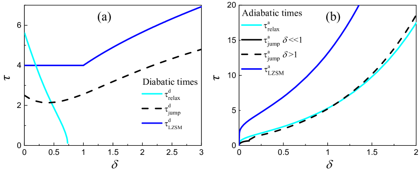
Figure 19: Transition times $t_{\text{jump}}$ and $t_{\text{relax}}$ versus the adiabaticity parameter $\delta$. Here, the dimensionless time is $\tau=t\left[v/2\hbar\right]^{1/2}$. Note that in the adiabatic basis $t_{\text{jump}}^{\text{a}}\approx t_{\text{relax}}^{\text{a}}$, and also that these transition times grow exponentially in the adiabatic limit ($\delta\gg 1$). In the diabatic basis and the diabatic limit ($\delta\ll 1$) $t_{\text{relax}}^{\text{d}}>t_{\text{jump}}^{\text{d}}$, and there is no $t_{\text{relax}}^{\text{d}}$ in the adiabatic limit. Note that $\tau_{\text{LZSM}}$ is plotted using Eq. (21a) and (21b).

For the jump and relaxation times in the adiabatic basis, from Eqs. (151) and (181), it follows

$$t_{\text{jump}}^{\text{a}}\approx\begin{cases}4\sqrt{\frac{\hbar\delta}{v}}\text{, \ \ }\delta\ll 1,\\ \sqrt{\frac{2}{v}}\left(\frac{1}{\eta}8\delta\exp\left[4\pi\delta\right]\right)^{1/6}\text{, \ \ }\delta\gg 1,\end{cases}$$ (185a)

and

$$t_{\text{relax}}^{\text{a}}\approx\sqrt{\frac{4\delta}{v}\left[\left(\frac{e^{2\pi\delta}-1}{16\eta^{2}\delta^{4}}\right)^{1/3}-1\right]}.$$ (185b)

In the limiting cases for the relaxation time, we then have

$$t_{\text{relax}}^{\text{a}}\approx\begin{cases}\sqrt{\frac{2}{v}}(2\delta/\eta)^{1/3}\text{, \ \ }\delta\ll 1,\\ \\ \sqrt{\frac{2}{v}}\left(\frac{\exp\left[\pi\delta\right]}{\eta}\right)^{1/3}(\delta/2)^{1/6}\text{, \ \ }\delta\gg 1.\end{cases}$$ (185c)

We show the transition times in Fig. 19. To plot these, we have used Eq. (184c) for $t_{\text{relax}}^{\text{d}}$ and Eq. (184a) for $t_{\text{jump}}^{\text{d}}$ in Fig. 19(a); then, we used Eq. (185b) for $t_{\text{relax}}^{\text{a}}$ and Eq. (185c) for $t_{\text{jump}}^{\text{a}}$ in Fig. 19(b).

Here, for $\delta\ll 1$, we have $t_{\text{relax}}^{\text{d}}\gg t_{\text{relax}}^{\text{a}}$. This difference in the relaxation times happens because the oscillations of $P_{\text{d}}(t)$ vanish proportionally to $t^{-1}$, but $P_{\text{a}}(t)$ decays proportionally to $t^{-3}$.

For the case $\delta\gg 1$, we have the opposite situation: $t_{\text{relax}}^{\text{a}}\gg t_{\text{relax}}^{\text{d}}\approx 0$. Note that $t_{\text{relax}}^{\text{a}}\approx t_{\text{jump}}^{\text{a}}$; therefore, we can define $t_{\text{LZSM}}\approx 2t_{\text{relax}}^{\text{a}}$. As a result, the equations above can be summarized as Eqs. (21a, 21b) in the main text.

Appendix B Description of a periodically driven two-level system

B.1 Adiabatic-impulse model (AIM)

In this section, we describe the adiabatic-impulse model in more detail, expanding on Section III.1.

B.1.1 Adiabatic evolution

Consider now the adiabatic evolution when the system passes in one of the adiabatic eigenstates $\left|E_{\pm}(t)\right\rangle$. This means that the adiabatic basis consists of the instantaneous eigenstates of the time-dependent Hamiltonian. We can obtain the instantaneous eigenfunctions from the Schrödinger equation (118), where time $t$ is a parameter:

$$H(t)\left|E_{\pm}(t)\right\rangle=E_{\pm}(t)\left|E_{\pm}(t)\right\rangle.$$ (186)

To describe the system dynamics, we solve the dynamical form of the Schrödinger equation, Eq. (15), with the initial condition

$$\left|E_{\pm}(t_{\text{i}})\right\rangle=\left|E_{\text{i}\pm}\right\rangle.$$ (187)

We substitute Eq. (186) into the Schrödinger equation (15), solve this differential equation, and then obtain the evolution of the upper- and lower-energy-level wave functions

$$\left|E_{\pm}(t)\right\rangle = \exp{\left(-\frac{i}{\hbar}\int_{t_{\text{i}}}^{t}E_{\pm}(t^{\prime})dt^{\prime}\right)}\left|E_{\text{i}\pm}\right\rangle=\exp{\left(\mp i\zeta\right)}\left|E_{\text{i}\pm}\right\rangle,$$ (188a)

$$\zeta(t) = \frac{1}{2\hbar}\int_{t_{\text{i}}}^{t}\Delta E(t)\;dt.$$ (188b)

As a result, we obtain the adiabatic evolution matrix, Eq. (27).

B.1.2 Multiple-passage evolution

Here we describe some aspects of the multiple-passage evolution in relation to Sec. III.1. To raise the matrix $\Xi$ to the $n$-th power [see Eq. (48)], we first need to diagonalize it. For this, we use the unitary matrix

$$A=\begin{pmatrix}A_{11}&-A_{21}^{\ast}\\ A_{21}&A_{11}^{\ast}\end{pmatrix},\;\;\text{ }AA^{\dagger}=1,\;\;\text{ }|A_{11}|^{2}+|A_{21}|^{2}=1,$$ (189)

such that $A\Xi A^{\dagger}=\begin{pmatrix}e^{i\phi}&0\\ 0&e^{-i\phi}\end{pmatrix}$, where $\phi$ is the desired value. Consider the equation $\Xi=A^{\dagger}\begin{pmatrix}e^{i\phi}&0\\ 0&e^{-i\phi}\end{pmatrix}A$ and obtain

$$\begin{cases}\Xi_{11}=|A_{11}|^{2}e^{i\phi}+|A_{21}|^{2}e^{-i\phi}\\ \Xi_{21}=-2iA_{11}A_{21}\sin\phi.\end{cases}$$ (190)

From these, we define $\phi$: $\cos\phi=$Re$\Xi_{11}$. In the next step, we find the matrix $\Xi_{n}$ of the evolution for $n$ periods

$$\Xi_{n}=\Xi^{n}=A^{\dagger}\begin{pmatrix}e^{in\phi}&0\\ 0&e^{-in\phi}\end{pmatrix}A=\begin{pmatrix}\Xi_{n11}&-\Xi_{n21}^{\ast}\\ \Xi_{n21}&\Xi_{n11}^{\ast}\end{pmatrix},$$ (191a)

where we simplify the obtained matrix elements, here taking into account Eq. (190):

$$\Xi_{n11} = \cos(n\phi)+i\text{{Im}}(\Xi_{11})\frac{\sin{(n\phi)}}{\sin\phi},$$ (191b)

$$\Xi_{n21} = \Xi_{21}\frac{\sin{(n\phi)}}{\sin\phi}.$$ (191c)

Then, we obtain the probability of the upper-level occupation of the TLS during their respective time intervals:

$$P_{+}^{(1)}(n) = \left|\Xi_{n21}\right|^{2}=\left|\Xi_{21}\right|^{2}\frac{\sin^{2}{n\phi}}{\sin^{2}\phi},\;\;\ \ \ \text{ for }(t-nT_{\mathrm{d}})\in(t_{2},T_{\mathrm{d}}+t_{1}),$$ (192a)

$$P_{+}^{(2)}(n) = 2Q_{1}\frac{\sin^{2}{n\phi}}{\sin^{2}\phi}+Q_{2}\frac{\sin{2n\phi}}{\sin\phi}+\mathcal{P}\cos{2n\phi},\;\;\ \ \ \text{ for }(t-nT_{\mathrm{d}})\in(t_{1},t_{2}),$$ (192b)

where

$$Q_{1}=\mathcal{P}\left[\mathcal{P}\sin^{2}{\zeta_{-}}+(1-\mathcal{P})(1+\cos{\zeta_{+}}\cos{\zeta_{-}})\right],$$ (192c)

$$Q_{2}=2\mathcal{P}(1-\mathcal{P})\cos{(\zeta_{1}+{\phi}_{\text{S}})}\cos{(\zeta_{2}+{\phi}_{\text{S}})}.$$ (192d)

For the time-averaged value, we need to average over many periods $n\gg 1$, so we obtain

$$\overline{P_{+}^{(1)}} = \frac{|\Xi_{21}|^{2}}{2\sin^{2}{\phi}}=\frac{1}{2}\frac{|\Xi_{21}|^{2}}{|\Xi_{21}|^{2}+(\text{{Im}}{\Xi_{11}})^{2}},$$ (193a)

$$\overline{P_{+}^{(2)}} = \frac{Q_{1}}{\sin^{2}{\phi}}.$$ (193b)

We can neglect the difference between $\overline{P_{+}^{(1)}}$ and $\overline{P_{+}^{(2)}}$ in the case of the slow-passage limit $\mathcal{P}\ll 1$, that is, $\delta\gg 1$. Here, we use $\mathcal{P}$ as a small parameter, and in the first approximation, we obtain Eq. (60).

B.2 Rotating-wave approximation (RWA)

Consider now the case of strong excitation, $\Delta\ll\sqrt{A\hbar\omega}$ at $k\hbar\omega\approx\Delta E$, where the latter condition means that the energy of $k$ photons approximately equals the energy distance between the qubit levels $\Delta E$. Here, we follow Refs. Silveri et al. (2015); Ono et al. (2019) presenting the formalism valid not only for the cosine driving but rather for a generic excitation $\varepsilon(t)=\varepsilon_{0}+\widetilde{\varepsilon}(t)$ for any function $\widetilde{\varepsilon}(t)$ with the period $T_{\mathrm{d}}=2\pi/\omega$.

Let us first split the Hamiltonian into a stationary part $H_{0}$ and a time-dependent part $V(t)$:

$$H=H_{0}+V(t)=-\frac{\Delta}{2}\sigma_{x}-\frac{\varepsilon_{0}}{2}\sigma_{z}-\frac{\widetilde{\varepsilon}(t)}{2}\sigma_{z}.$$ (194)

To make it convenient to solve the Bloch equations, we perform the unitary transformation:

$$U=\exp\left[-i\frac{\eta(t)}{2}\sigma_{z}\right]=\cos{\frac{\eta}{2}}-i\sigma_{z}\sin{\frac{\eta}{2}},\;\;\;\;\;\eta(t)=\frac{1}{\hbar}\int_{0}^{t}dt^{\prime}\;\widetilde{\varepsilon}\left(t^{\prime}\right).$$ (195)

We use the operator $U(t)$ to link the wave function in the rotating and stationary coordinate systems, $\psi=U(t)\psi^{\prime}$. Then, we substitute this function into the Schrödinger equation and obtain $i\hbar U\dot{\psi}^{\prime}+i\hbar\dot{U}\psi^{\prime}=HU\psi^{\prime}$. In the rotating coordinate system, we need $i\hbar\dot{\psi}^{\prime}=H^{\prime}\psi^{\prime}$, thus obtaining the new Hamiltonian

$$H^{\prime}=\!U^{{\dagger}}HU-i\hbar U^{{\dagger}}\dot{U}=-\frac{\varepsilon_{0}}{2}\sigma_{z}-\frac{\Delta}{2}\left(e^{i\eta}\sigma_{+}+h.c.\right),$$ (196)

with $\sigma_{+}=\frac{1}{2}\left(\sigma_{x}+i\sigma_{y}\right)$. Then, the preparatory stage is finalized by the Fourier series expansion

$$\Delta e^{i\eta}=\sum_{m=-\infty}^{\infty}\Delta_{m}\,e^{im\omega t},$$ (197)

where the complex-valued amplitude is given by the inverse Fourier transform

$$\Delta_{m}=\Delta\frac{\omega}{2\pi}\int\limits_{0}^{2\pi/\omega}dt\;e^{-im\omega t}e^{i\eta(t)}=\Delta\int\limits_{0}^{1}d\tau^{\prime}\exp\left[i\eta(\tau^{\prime})-i2\pi m\tau^{\prime}\right].$$ (198)

Then, the Hamiltonian becomes

$$H^{\prime}=\!-\frac{\varepsilon_{0}}{2}\sigma_{z}+\frac{1}{2}\sum_{m=-\infty}^{\infty}\left(\Delta_{m}e^{im\omega t}\sigma_{+}+h.c.\right)=-\frac{1}{2}\sum_{m=-\infty}^{\infty}\begin{pmatrix}\varepsilon_{0}&\Delta_{m}e^{im\omega t}\\ \Delta_{m}e^{-im\omega t}&-\varepsilon_{0}\end{pmatrix}.$$ (199)

With this Hamiltonian, it is convenient to solve the Bloch equations for the density matrix,

$$\dot{\rho}_{ij}=-\frac{i}{\hbar}\left[H,\rho\right]_{ij}-\frac{\rho_{ij}-\rho_{ij}^{(0)}}{\tau_{ij}},$$ (200)

where $\rho_{ij}$ is the density matrix, $\tau_{ij}$ is the relaxation rate, $\rho^{(0)}$ is the equilibrium density operator with $\rho_{01}^{(0)}=\rho_{10}^{(0)}=0$, $Z^{(0)}=~{}\rho_{00}^{(0)}-~{}\rho_{11}^{(0)}=~{}\tanh\frac{\Delta E}{2k_{B}T}$, and $k_{B}$ is the Boltzmann constant. For this, we parameterize the density matrix

$$\rho=\frac{1}{2}\left(1\sigma_{0}+X\sigma_{x}+Y\sigma_{y}+Z\sigma_{z}\right)=\frac{1}{2}\begin{pmatrix}1+Z&X-iY\\ X+iY&1-Z\end{pmatrix}\equiv\begin{pmatrix}\rho_{00}&\rho_{01}\\ \rho_{10}&\rho_{11}\end{pmatrix}.$$ (201)

For the moment, we assume that the system is driven close to a resonance, where $\Delta E\approx\left|\varepsilon_{0}\right|\approx k\hbar\omega$. Then, we omit the “fast-rotating” terms and leave only terms with $m=k$. We can write down the Bloch equations with the Hamiltonian $H^{\prime}$ component-wise:

$$\dot{Z} = -\frac{\Delta_{k}}{2\hbar}\mathrm{Im}(e^{-ik\omega t})-(Z-Z^{(0)})\Gamma_{1},$$ (202a)

$$\dot{\rho}_{10} = i\frac{\Delta_{k}}{2\hbar}e^{ik\omega t}Z-i\frac{\varepsilon_{0}}{\hbar}\rho_{10}-\rho_{10}\Gamma_{2},$$ (202b)

where

$$Z^{(0)}=\rho_{00}^{(0)}-\rho_{11}^{(0)}=\tanh\frac{\Delta E}{2k_{\text{B}}T}.$$ (202c)

Here $\Delta_{k}$ was defined in Eq. (72). After the substitution $\rho_{10}\exp{\left(-ik\omega t\right)}=\widetilde{X}+i\widetilde{Y}$, we obtain the system of equations

$$\dot{\widetilde{X}} = \left(k\omega+\frac{\varepsilon_{0}}{\hbar}\right)\widetilde{Y}-\widetilde{X}\Gamma_{2},$$ (203a)

$$\dot{\widetilde{Y}} = -\left(k\omega+\frac{\varepsilon_{0}}{\hbar}\right)\widetilde{X}+\frac{\Delta_{k}}{\hbar}Z-\widetilde{Y}\Gamma_{2},$$ (203b)

$$\dot{Z} = -\frac{\Delta_{k}}{\hbar}\widetilde{Y}-(Z-Z^{(0)})\Gamma_{1}.$$ (203c)

The stationary solution of these equations can be obtained after substituting $\dot{\widetilde{X}}=\dot{\widetilde{Y}}=\dot{Z}=0$. Consider now the low-temperature case, $T\rightarrow 0$, then $Z^{(0)}\approx 1$. Finally, we obtain the stationary value for the probability of the upper diabatic state; summing all possible resonant terms, we obtain the qubit upper-level occupation probability

$$\overline{P}_{\mathrm{up}}^{(k)} = \overline{\rho}_{11}^{(k)}=\frac{1}{2}\left(1-\overline{Z}^{(k)}\right),$$ (204a)

$$\overline{P}_{\mathrm{up}} = \sum_{k}\overline{P}_{\mathrm{up}}^{(k)}=\frac{1}{2}\sum_{k=-\infty}^{\infty}\frac{\left|\Delta_{k}\right|^{2}}{\left|\Delta_{k}\right|^{2}+\frac{\Gamma_{1}}{\Gamma_{2}}\left(k\hbar\omega-\varepsilon_{0}\right)^{2}+\hbar^{2}\Gamma_{1}\Gamma_{2}}.$$ (204b)

Note that for a complex-valued $\Delta_{k}$, what matters is its absolute value.

Finally, to obtain the upper-level occupation probability for a given bias $\widetilde{\varepsilon}(t)$, we must calculate the functions $\Delta_{k}$. Although more examples can be seen in Silveri et al. (2015); Ono et al. (2019), for the sinusoidal modulation, with the Jacobi–Anger expansion following Eq. (72), it is straightforward to see that

$$\Delta_{m}(x)=\Delta J_{m}(x),\;\;\;\;x=\frac{A}{\hbar\omega}.$$ (205)

It is useful to recall here the asymptote at $x\gg 1$:

$$J_{m}(x)\approx\sqrt{\frac{2}{\pi x}}\cos\left[x-\frac{\pi m}{2}-\frac{\pi}{4}\right].$$ (206)

This explicitly demonstrates that the occupation probability is quasiperiodic in driving the amplitude with the period $\delta A=2\pi\hbar\omega$.

B.3 Floquet theory

From Floquet theory Son et al. (2009), we can obtain a solution $\left|\psi(t)\right\rangle$ for the Schrödinger equation (15) with any time-periodic Hamiltonian $H(t)=H(t+nT_{\mathrm{d}})$ for any integer $n$

$$\left|\psi(t)\right\rangle=e^{-i\epsilon t}\left|\Phi(t)\right\rangle,$$ (207)

where $\left|\Phi(t)\right\rangle$ denote the time-periodic Floquet modes with the same period as the Hamiltonian $H(t)$ and $\epsilon$ is the so-called quasienergy. When we substitute Eq. (207) into Eq. (15), we can obtain an equation for the quasienergy

$$\left(H(t)-i\hbar\frac{d}{dt}\right)\left|\Phi(t)\right\rangle=\epsilon\left|\Phi(t)\right\rangle.$$ (208)

Periodic functions can be decomposed into harmonic functions using the Fourier series expansion

$$\left|\Phi(t)\right\rangle = \sum_{n=-\infty}^{\infty}\left|\Phi_{n}\right\rangle e^{in\omega t},$$ (209a)

$$H(t) = \sum_{n=-\infty}^{\infty}H^{[n]}e^{in\omega t},$$ (209b)

where the superscript $$[n]$$ defines the number of the 2x2 part of the Hamiltonian matrix. For the next step, we rewrite the Hamiltonian in its exponential form

$$H(t)=-\frac{\Delta}{2}\sigma_{x}-\frac{\varepsilon_{0}}{2}\sigma_{z}-\frac{A}{4}\sigma_{z}\left(e^{i\omega t}+e^{-i\omega t}\right),$$ (210)

and we obtain the system of stationary equations for the quasienergies using the Schrödinger equation (15) with the substitutions (207) and (209)

$$\sum_{i}\sum_{m}\langle 0,n|H_{\mathrm{F}}|i,m\rangle\langle i,m|\epsilon_{j}\rangle=\epsilon_{j}\langle 0,n|\epsilon_{j}\rangle,$$ (211)

where $H_{\mathrm{F}}$ is the Floquet Hamiltonian, $\epsilon_{j}$ is the quasienergy eigenvalue, $|\epsilon_{j}\rangle$ is an eigenvector, and $\left|i,m\right\rangle$ is the $m$-th Fourier component of the $i$-th energy level. We can also write it in terms of matrix elements

$$\epsilon_{j}\Phi_{j,n}=\left(-\frac{\Delta}{2}\sigma_{x}-\frac{\varepsilon_{0}}{2}\sigma_{z}+n\omega\right)\Phi_{n}-\frac{A}{4}\sigma_{z}\left(\Phi_{n-1}+\Phi_{n+1}\right),$$ (212)

where $j$ defines the number of a state, which is either $0$ or $1$ for a TLS after decomposing the wave function, Eq. (3). Then, we obtain the time-independent Floquet Hamiltonian, which is defined by

$$\left\langle i_{n}\right|H_{\mathrm{F}}\left|j_{k}\right\rangle=H_{0,1}^{[n-k]}+n\hbar\omega\delta_{ij}\delta_{nk},$$ (213a)

where $$i j$$ and define the number of the state, or

$$H_{\mathrm{F},nk}=H^{[n-k]}+n\hbar\omega\delta_{nk}I,$$ (213b)

for 2x2 elements ($$I H^{\left[n-k\right]} n ~{}k$$ is 2x2 identity matrix) with three nonvanishing Fourier components of the Hamiltonian , where and are the integer numbers corresponding to different states:

$$H^{[0]}=-\frac{1}{2}\begin{pmatrix}\varepsilon_{0}&\Delta\\ \Delta&-\varepsilon_{0}\end{pmatrix},\text{ \ }H^{[+1]}=H^{[-1]}=-\frac{1}{4}\begin{pmatrix}A&0\\ 0&-A\end{pmatrix}.$$ (214)

This consists of the 2x2 submatrices, and Eq. (213b) defines its element in the $n$-th column and the $k$-th row. Hence, the Floquet states matrix can be written as

$$H_{\mathrm{F}}=\left(\begin{array}[]{c|cc|cc|cc|c}\ddots&&&&&&&\\ \hline\cr&\rule{0.0pt}{17.22217pt}-\frac{\varepsilon_{0}}{2}+(n-1)\hbar\omega&-\frac{\Delta}{2}&-\frac{A}{4}&0&0&0&\\ &\rule{0.0pt}{17.22217pt}-\frac{\Delta}{2}&\frac{\varepsilon_{0}}{2}+(n-1)\hbar\omega&0&\frac{A}{4}&0&0&\\[8.61108pt] \hline\cr&\rule{0.0pt}{17.22217pt}-\frac{A}{4}&0&-\frac{\varepsilon_{0}}{2}+n\hbar\omega&-\frac{\Delta}{2}&-\frac{A}{4}&0&\\ &\rule{0.0pt}{17.22217pt}0&\frac{A}{4}&-\frac{\Delta}{2}&\frac{\varepsilon_{0}}{2}+n\hbar\omega&0&\frac{A}{4}&\\[8.61108pt] \hline\cr&\rule{0.0pt}{17.22217pt}0&0&-\frac{A}{4}&0&-\frac{\varepsilon_{0}}{2}+(n+1)\hbar\omega&-\frac{\Delta}{2}&\\ &\rule{0.0pt}{17.22217pt}0&0&0&\frac{A}{4}&-\frac{\Delta}{2}&\frac{\varepsilon_{0}}{2}+(n+1)\hbar\omega&\\[8.61108pt] \hline\cr&&&&&&&\ddots\end{array}\right).$$ (215)

The eigenvalues of this matrix can be found numerically if we take a finite number of these 2x2 blocks. Then, we can obtain the time-averaged upper-level occupation probability

$$\overline{P}_{\mathrm{up}}=\sum_{n}\sum_{j}|\left\langle 1_{n}|\epsilon_{j}\right\rangle\left\langle\epsilon_{j}|0_{(n=0)}\right\rangle|^{2}.$$ (216)

The Schrödinger equation with the Hamiltonian $H_{\mathrm{F}}$ in the general case cannot be solved analytically; therefore, we first consider the eigenvalue problem with $\Delta=0$; next, we can use perturbation theory with the small parameter being $\Delta$. We denote $H_{0}$ as the unperturbed Hamiltonian. In the situation when $\Delta=0$, there is no coupling between the $\left|0\right\rangle$ and $\left|1\right\rangle$ states; therefore we can write the same Hamiltonian $H_{0}^{\prime}$ for both states:

$$\widetilde{H}_{0}(\text{for state }0\text{ or }1)=\begin{pmatrix}\ddots&&&&\\ &b+(n-1)\hbar\omega&a&0&\\ &a&b+n\hbar\omega&a&\\ &0&a&b+(n+1)\hbar\omega&\\ &&&&\ddots\end{pmatrix}$$ (217)

where $b=-\frac{\varepsilon_{0}}{2}$, $a=-\frac{A}{4}$ for the $\left|0\right\rangle$ state and $b=\frac{\varepsilon_{0}}{2}$, $a=\frac{A}{4}$ for the $\left|1\right\rangle$ state. To find the eigenfunctions, we use the Schrödinger equation (208) with Hamiltonian $\widetilde{H}_{0}^{\prime},$ in which $\Delta=0$. As a result, using the Jacobi–Anger formula (205), we obtain

$$|\widetilde{\Phi}_{n}(t)\rangle=e^{in\omega t}e^{-i(2a/\hbar\omega)\sin\omega t}=\sum_{k=-\infty}^{\infty}J_{k}\left(-\frac{2a}{\hbar\omega}\right)e^{i(n+k)\omega t}=\sum_{k=-\infty}^{\infty}J_{k-n}\left(\frac{A}{2\hbar\omega}\right)e^{-ik\omega t}.$$ (218)

The eigenstates of the unperturbed Hamiltonian $H_{0}$ are the following:

$$\left|\widetilde{0},n\right\rangle = \sum_{k=-\infty}^{\infty}J_{k-n}\left(\frac{A}{2\hbar\omega}\right)\left|0,k\right\rangle,$$ (219a)

$$\left|\widetilde{1},m\right\rangle = \sum_{k=-\infty}^{\infty}J_{k-m}\left(-\frac{A}{2\hbar\omega}\right)\left|1,m\right\rangle.$$ (219b)

For the Floquet Hamiltonian (215), using the addition theorem for Bessel functions

$$J_{n}(2z)=\sum_{m}J_{m}(z)J_{n-m}(z),$$ (220)

we can obtain the matrix elements for the Floquet Hamiltonian based on this (215):

$$\left\langle 0_{n}^{\prime}\right|H_{\mathrm{F}}\left|1_{m}^{\prime}\right\rangle = \sum_{k=-\infty}^{\infty}\sum_{l=-\infty}^{\infty}J_{k-n}(z)J_{l-m}(-z)\left\langle 0_{k}\right|H_{F}\left|1_{l}\right\rangle=-\frac{\Delta}{2}J_{m-n}\left(\frac{A}{\hbar\omega}\right),$$ (221a)

$$\left\langle 1_{n}^{\prime}\right|H_{\mathrm{F}}\left|0_{m}^{\prime}\right\rangle = -\frac{\Delta}{2}J_{n-m}\left(\frac{A}{\hbar\omega}\right),$$ (221b)

$$\left\langle 0_{n}^{\prime}\right|H_{\mathrm{F}}\left|0_{m}^{\prime}\right\rangle = \left(-\frac{\varepsilon_{0}}{2}+n\hbar\omega\right)\delta_{nm},$$ (221c)

$$\left\langle 1_{n}^{\prime}\right|H_{\mathrm{F}}\left|1_{m}^{\prime}\right\rangle = \left(\frac{\varepsilon_{0}}{2}+n\hbar\omega\right)\delta_{nm}.$$ (221d)

From Eqs. (221), if we have the condition for the multi-photon resonances, $$\varepsilon_{0}\approx n\hbar\omega \left|0_{0}^{\prime}\right\rangle \left|1_{-n}^{\prime}\right\rangle$$, then we can neglect all other coupling terms, except the one between and ; therefore, we obtain a 2x2 matrix Hamiltonian:

$$H_{\text{RWA}}=-\frac{1}{2}\begin{pmatrix}\varepsilon_{0}&\Delta J_{-n}^{\prime}\\ \Delta J_{-n}^{\prime}&-\varepsilon_{0}+\frac{n\hbar\omega}{2}\end{pmatrix}$$ (222a)

where

$$J_{n}^{\prime}=J_{n}\left(\frac{A}{\hbar\omega}\right).$$ (222b)

Generalized Van Vleck Perturbation Theory

The RWA is the first approximation in Floquet theory; for the next approximations, we can use generalized Van Vleck perturbation theory (GVVPT) Son et al. (2009). The perturbation (small) parameter is

$$\lambda=-\frac{\Delta}{2}.$$ (223)

Here, we can rewrite the Floquet Hamiltonian in the basis of the states $\left|0_{n}^{\prime}\right\rangle$ and $\left|1_{m}^{\prime}\right\rangle$:

$$\widetilde{H}_{\mathrm{F}}=\widetilde{H}_{0}^{\prime}+\lambda\widetilde{V},$$ (224a)

where

$$\widetilde{H}_{0}^{\prime} = \left(\begin{array}[]{c|cc|cc|cc|c}\ddots&&&&&&&\\ \hline\cr&\rule{0.0pt}{4.30554pt}-\frac{\varepsilon_{0}}{2}-\hbar\omega&0&0&0&0&0&\\ &0&\frac{\varepsilon_{0}}{2}-\hbar\omega&0&0&0&0&\\[4.30554pt] \hline\cr&0&0&-\frac{\varepsilon_{0}}{2}&0&0&0&\\ &0&0&0&\frac{\varepsilon_{0}}{2}&0&0&\\ \hline\cr&0&0&0&0&-\frac{\varepsilon_{0}}{2}+\hbar\omega&0&\\ &0&0&0&0&0&\frac{\varepsilon_{0}}{2}+\hbar\omega&\\ \hline\cr&&&&&&&\ddots\end{array}\right),$$ (224j)

$$\widetilde{V} = \begin{pmatrix}\begin{array}[]{c|cc|cc|cc|c}\ddots&&&&&&&\\ \hline\cr&0&J_{0}^{\prime}&0&J_{1}^{\prime}&0&J_{2}^{\prime}&\\ &J_{0}^{\prime}&0&J_{-1}^{\prime}&0&J_{-2}^{\prime}&0&\\ \hline\cr&0&J_{-1}^{\prime}&0&J_{0}^{\prime}&0&J_{1}^{\prime}&\\ &J_{1}^{\prime}&0&J_{0}^{\prime}&0&J_{-1}^{\prime}&0&\\ \hline\cr&0&J_{-2}^{\prime}&0&J_{-1}^{\prime}&0&J_{0}^{\prime}&\\ &J_{2}^{\prime}&0&J_{1}^{\prime}&0&J_{0}^{\prime}&0&\\ \hline\cr&&&&&&&\ddots\end{array}\end{pmatrix}.$$ (224k)

We can reduce the infinite-dimensional matrix of the Floquet Hamiltonian (215) to a 2x2 matrix Hamiltonian $h$ by using the nearly degenerate perturbation formalism in the GVVPT Aravind and Hirschfelder (1984). Following perturbation theory, the 2x2 matrix of Hamiltonian $h$ and its eigenstates solutions $\phi$ can be expanded in powers of $\lambda$

$$h = \sum_{m=0}^{\infty}\lambda^{m}h^{(m)},$$ (225a)

$$\phi = \sum_{m=0}^{\infty}\lambda^{m}\phi^{(m)}.$$ (225b)

For the $$n$$-photon resonance, the Floquet states are nearly degenerate, so

$$\phi_{-}^{(0)}=\left|\widetilde{0}_{0}\right\rangle\text{ and }\phi_{+}^{(0)}=\left|\widetilde{1}_{0}\right\rangle$$ (226a)

and

$$h^{(0)}=\frac{1}{2}\begin{pmatrix}-\varepsilon_{0}&0\\ 0&\varepsilon_{0}-2n\hbar\omega\end{pmatrix},$$ (226b)

where the two states are nearly degenerate, that is, $\varepsilon_{0}\approx n\hbar\omega$. Using GVVPT, a few high-order terms can be obtained:

$$\phi_{-}^{(1)} = \sum\nolimits_{k}^{\prime}\frac{-J_{k}^{\prime}}{\varepsilon_{0}+k\hbar\omega}\left|\widetilde{1}_{k}\right\rangle,$$ (227a)

$$\phi_{+}^{(1)} = \sum\nolimits_{k}^{\prime}\frac{J_{k}^{\prime}}{\varepsilon_{0}+k\hbar\omega}\left|\widetilde{1}_{-n-k}\right\rangle,$$ (227b)

$$h^{(1)} = \left\langle\phi^{(0)}|V^{\prime}|\phi^{(0)}\right\rangle=J_{-}^{\prime}\begin{pmatrix}0&1\\ 1&0\end{pmatrix},$$ (227c)

$$h^{(2)} = \left\langle\phi^{(0)}|V^{\prime}|\phi^{(1)}\right\rangle-h^{(1)}\left\langle\phi^{(0)}|\phi^{(1)}\right\rangle=\sum\nolimits_{k}^{\prime}\frac{J_{k}^{\prime 2}}{\varepsilon_{0}+k\hbar\omega}\begin{pmatrix}-1&0\\ 0&1\end{pmatrix},$$ (227d)

$$h^{(3)} = \left\langle\phi^{(1)}|V^{\prime}|\phi^{(1)}\right\rangle-\left\langle\phi^{(1)}|\phi^{(1)}\right\rangle h^{(1)}=-\sum\nolimits_{k}^{\prime}\left(\sum\nolimits_{l}^{\prime}\frac{J_{k}^{\prime}J_{l}^{\prime}J_{k+l+n}^{\prime}}{\left(\varepsilon_{0}+k\hbar\omega\right)\left(\varepsilon_{0}+l\hbar\omega\right)}+\frac{J_{k}^{\prime 2}J_{-n}^{\prime}}{\left(\varepsilon_{0}+k\hbar\omega\right)^{2}}\right)\begin{pmatrix}0&1\\ 1&0\end{pmatrix}.$$ (227e)

Here, the summation $$\sum\nolimits_{k}^{\prime} -\infty \infty k\neq-n n$$ is from to , with the prime standing for . As a result of GVVPT, we obtain the Hamiltonian, which includes -photon coupling channels

$$H_{\text{GVVPT}}=\frac{1}{2}\begin{pmatrix}-\varepsilon_{0}-\delta_{n}&\widetilde{\Delta}_{n}\\ \widetilde{\Delta}_{n}&\varepsilon_{0}+\delta_{n}-2n\hbar\omega\end{pmatrix},$$ (228)

where

$$\widetilde{\Delta}_{n} = J_{-n}^{\prime}2\lambda-\sum\nolimits_{k}^{\prime}\left(\sum\nolimits_{l}^{\prime}\frac{J_{k}^{\prime}J_{l}^{\prime}J_{k+l+n}^{\prime}}{\left(\varepsilon_{0}+k\hbar\omega\right)\left(\varepsilon_{0}+l\hbar\omega\right)}+\frac{J_{k}^{\prime 2}J_{-n}^{\prime}}{\left(\varepsilon_{0}+k\hbar\omega\right)^{2}}\right)2\lambda^{3}+O(\lambda^{5}),$$ (229a)

$$\delta_{n} = \sum\nolimits_{k}^{\prime}2\frac{J_{k}^{\prime 2}}{\varepsilon_{0}+k\hbar\omega}\lambda^{2}+O(\lambda^{4}).$$ (229b)

Then, we find the eigenvalues of the GVVPT Hamiltonian (228)

$$\epsilon_{0,1}=-\frac{n\hbar\omega}{2}\pm\hbar\widetilde{\Omega}_{\text{R}},$$ (230a)

where

$$\left(\hbar\widetilde{\Omega}_{\text{R}}\right)^{2}=(n\hbar\omega-\varepsilon_{0}-\delta_{n})^{2}+\widetilde{\Delta}_{n}^{2}.$$ (230b)

This gives the $n$-photon time-dependent upper-level occupation probability

$$P_{\text{up}}^{(n)}(t)=\frac{1}{2}\frac{\widetilde{\Delta}_{n}^{2}}{\left(\hbar\widetilde{\Omega}_{\text{R}}\right)^{2}}\left(1-\cos\widetilde{\Omega}_{\text{R}}t\right),$$ (231)

and averaged occupation probability

$$\overline{P}_{\text{up}}^{(n)}=\lim_{t\rightarrow\infty}\frac{1}{t}\int_{0}^{t}P_{\text{up}}^{(n)}(t^{\prime})dt^{\prime}=\frac{1}{2}\frac{\widetilde{\Delta}_{n}^{2}}{\widetilde{\Delta}_{n}^{2}+(n\hbar\omega-\varepsilon_{0}-\delta_{n})^{2}}.$$ (232)

When we take only the first term of this, we can reach the RWA limit

$$\overline{P}_{\text{up}}^{(n)}=\frac{1}{2}\frac{\Delta_{n}^{2}}{\Delta_{n}^{2}+(n\hbar\omega-\varepsilon_{0})^{2}},$$ (233)

where $\Delta_{n}$ is the same as in the RWA and as was defined in Eq. (205).

B.4 Rate-equation and white-noise approach

In this subsection, we describe a TLS dynamics modeling the decoherence by adding classical noise and then solving the rate equation. We demonstrate that such approach gives exactly the same solution as the one by solving the Bloch equation in the RWA.

B.4.1 Transition rate

Consider a transition rate in a driven TLS, following Berns et al. (2006) [see also Otxoa et al. (2019)]. This is described by the Hamiltonian

$$H(t)=-\frac{1}{2}\left(\begin{array}[]{cc}\varepsilon(t)&\Delta\\ \Delta&-\varepsilon(t)\end{array}\right),$$ (234a)

$$\varepsilon(t)=\varepsilon_{0}+A\cos\omega t+\delta\varepsilon(t),$$ (234b)

where $\delta\varepsilon(t)$ stands for classical noise, which models decoherence here.

After the unitary transformation

$$U=\exp\left(i\frac{\phi(t)}{2}\sigma_{z}\right),\text{ \ \ }\phi(t)=\frac{1}{\hbar}\int\limits_{0}^{t}dt^{\prime}\varepsilon(t^{\prime}),$$ (235)

we obtain

$$H^{\prime}(t)=U^{{\dagger}}HU-i\hbar U^{{\dagger}}\dot{U}=\left(\begin{array}[]{cc}0&\Delta(t)\\ \Delta^{\ast}(t)&0\end{array}\right),$$ (236a)

where

$$\Delta(t)=\Delta e^{-i\phi}.$$ (236b)

Perturbation theory gives the transition rate:

$$W=\lim_{\delta t\rightarrow\infty}\frac{\left|A_{t,t^{\prime}}\right|^{2}}{\delta t},\text{ \ \ }A_{t,t^{\prime}}=\frac{1}{2}\int\limits_{t}^{t^{\prime}}dt^{\prime}\,\Delta(t^{\prime}),\text{ \ \ }\delta t=t^{\prime}-t.$$ (237)

Here, the limit implies $\delta t\gg T_{2}$. Perturbation theory is valid, provided that the change of the qubit population is slow on the scale of $T_{2}$, which means that we have $W\ll T_{2}$ Berns et al. (2006); Danon and Rudner (2014).

We now add the averaging over white noise $\left\langle...\right\rangle_{\delta\varepsilon}$ and rewrite this:

$$W=\frac{1}{4}\lim_{\delta t\rightarrow\infty}\frac{1}{\delta t}\int\limits_{0}^{\tau}d\tau\int\limits_{t}^{t^{\prime}}dt^{\prime}\left\langle\Delta(t+\tau)\Delta^{\ast}(t^{\prime})\right\rangle_{\delta\varepsilon}.$$ (238)

Next, we use the Jacobi–Anger expansion, Eq. (205), to remove the sine from the exponent

$$e^{-i\phi(t)}=\exp\left(-i\frac{\varepsilon_{0}}{\hbar}t-i\frac{A}{\hbar\omega}\sin\omega t-i\delta\phi(t)\right)=e^{-i\frac{\varepsilon_{0}}{\hbar}t}e^{-i\delta\phi(t)}\sum_{n=-\infty}^{\infty}J_{n}(x)e^{-in\omega t}.$$ (239)

Here, we define

$$\delta\phi(t)=\frac{1}{\hbar}\int\limits_{0}^{t}dt^{\prime}\delta\varepsilon(t^{\prime})\text{ \ and\ \ }x=\frac{A}{\hbar\omega}.$$ (240)

If the noise is frequency independent (i.e., white) in a low-frequency region, the averaging gives Du et al. (2013b)

$$\left\langle e^{i\delta\phi(t)}e^{-i\delta\phi(t^{\prime})}\right\rangle_{\delta\varepsilon}=\exp{\left(-\Gamma_{2}\left|t-t^{\prime}\right|\right)}.$$ (241)

Then, calculating the integral

$$\int\limits_{-\infty}^{\infty}d\tau e^{-i\left(\frac{\varepsilon_{0}}{\hbar}-n\omega\right)\tau}e^{-\Gamma_{2}\left|\tau\right|}=\frac{2\Gamma_{2}}{\left(\frac{\varepsilon_{0}}{\hbar}-n\omega\right)^{2}+\Gamma_{2}^{2}},$$ (242)

we obtain the transition rate

$$W = \sum_{n=-\infty}^{\infty}W_{n},$$ (243a)

$$W_{n} = \frac{1}{2}\Gamma_{2}\frac{\Delta_{n}^{2}}{\left(\frac{\varepsilon_{0}}{\hbar}-n\omega\right)^{2}+\Gamma_{2}^{2}},$$ (243b)

$$\Delta_{n} = \Delta J_{n}(x).$$ (243c)

Note that the transition rate $W$ consists of the partial contributions $W_{n}$, each of which is essential in the vicinity of the $n$-th resonance, $\varepsilon_{0}\sim n\hbar\omega$.

B.4.2 Rate equation

The rate equation for a TLS reads

$$\frac{dP_{+}}{dt}=\left(W+\Gamma_{1}^{\prime}\right)P_{-}-\left(W+\Gamma_{1}\right)P_{+}.$$ (244)

Here, $\Gamma_{1}$ stands for the relaxation rate from the excited to the ground state, and $\Gamma_{1}^{\prime}=\Gamma_{1}\exp\left[-\Delta E/k_{\mathrm{B}}T\right]$ stands for the thermally-excited inverse relaxation. From this, it is apparent how to take temperature into account. In the following, we assume the low-temperature limit ($T=0$) and adopt $\Gamma_{1}^{\prime}=0$.

As the second equation, we can write down the equation for $dP_{-}/dt$, analogously to Eq. (244), or use the condition $P_{+}+P_{-}=1$. Then, in the stationary regime, with the zero left-hand side in Eq. (244), we obtain

$$P_{+}=\frac{W}{2W+\Gamma_{1}}\text{.}$$ (245)

In the vicinity of the $k$-th resonance, that is, at $\varepsilon_{0}\sim k\hbar\omega$, the probability is given by the $k$-th term $W_{k}$, Eq. (243b):

$$P_{+}^{(k)}=\frac{W_{k}}{2W_{k}+\Gamma_{1}}\text{.}$$ (246)

The summation of all possible resonances gives the full upper-level occupation probability:

$$P_{+}=\sum_{k=-\infty}^{\infty}P_{+}^{(k)}=\frac{1}{2}\sum_{k=-\infty}^{\infty}\frac{\Delta_{k}^{2}}{\Delta_{k}^{2}+\frac{\Gamma_{1}}{\Gamma_{2}}\left(\frac{\varepsilon_{0}}{\hbar}-k\omega\right)^{2}+\Gamma_{1}\Gamma_{2}}.$$ (247)

This exactly coincides with the solution of the Bloch equations in the RWA, Eq. (71).

B.4.3 From Bessel to Airy

It may be instructive to rewrite the Bessel function via the Airy function, as in Ref. Berns et al. (2006), (see also Ref. Malla and Raikh (2019))

$$J_{k}(x)\approx\sqrt[3]{\frac{2}{x}}\mathrm{Ai}\left(\sqrt[3]{\frac{2}{x}}\left(k-x\right)\right),$$ (248)

which is valid for $n\gg 1$ and $n>x$. Here, we can obtain Eq. (248) using Eqs. (8.455) and (8.433) from Ref. Gradshteyn and Ryzhik (2007) and the definition of the Airy function of the first kind, $\mathrm{Ai}\left(u\right)=\frac{1}{\pi}\int_{0}^{\infty}dt\cos\left(\frac{t^{3}}{3}+ut\right)$.

With this remark, we can proceed with the series in Eq. (243a). From the denominator in Eq. (243b), it follows that we can make the replacement in the nominator: $k\longrightarrow\varepsilon_{0}/\hbar\omega$; then, the respective Airy function goes out of the summation. We can execute the summation by expanding the fraction into two elementary fractions:

$$\frac{1}{\left(\frac{\varepsilon_{0}}{\hbar}-k\omega\right)^{2}+\Gamma_{2}^{2}}=\frac{1}{\Gamma_{2}\omega}\text{{Im}}\frac{1}{z-k},\ \ \ \ \text{ \ }z=\frac{\varepsilon_{0}}{\hbar\omega}-i\frac{\Gamma_{2}}{\omega}.$$ (249)

To calculate the sum, consider the expansion of the cotangent Gradshteyn and Ryzhik (2007) and its approximation for $\left|z\right|\gg 1$:

$$\cot\pi z=\frac{1}{\pi z}+\frac{1}{\pi}\sum_{k=-\infty}^{\infty}\frac{z}{k\left(z-k\right)}\approx\frac{1}{\pi}\sum_{k=-\infty}^{\infty}\frac{1}{z-k}.$$ (250)

As a result, we obtain

$$W\approx\frac{\pi\Delta^{2}}{2\hbar\omega}\left(\frac{2\hbar\omega}{A}\right)^{2/3}\mathrm{Ai}^{2}\left(\sqrt[3]{\frac{2\hbar\omega}{A}}\frac{\varepsilon_{0}-A}{\hbar\omega}\right)\times\text{{Im}}\cot\left[\pi\left(\frac{\varepsilon_{0}}{\hbar\omega}-i\frac{\Gamma_{2}}{\omega}\right)\right].$$ (251)

This formula, together with Eq. (245), is very convenient for further analysis of the upper-level occupation probability, of which the example follows.

B.4.4 Double-passage regime

Consider now the case when the decoherence rate is of the order of a driving period, $\Gamma_{2}\gtrsim\omega$. Then, $\cot(...)\approx i$ and, making use of Airy function asymptotics at a large negative argument (i.e., for the relevant $A>\varepsilon_{0}$), we obtain:

$$W\approx\frac{\pi\Delta^{2}}{2\hbar\omega}\sqrt[3]{\frac{4}{x^{2}}}\mathrm{Ai}^{2}\left(\sqrt[3]{\frac{2}{x}}\frac{\varepsilon_{0}-A}{\hbar\omega}\right)\approx\frac{1}{2}\frac{\Delta^{2}}{A}\left(1-\frac{\varepsilon_{0}}{A}\right)^{-1/2}\cos^{2}\left[\frac{2\sqrt{2}}{3}\frac{A}{\hbar\omega}\left(1-\frac{\varepsilon_{0}}{A}\right)^{3/2}-\frac{\pi}{4}\right].$$ (252)

Equation (252) can be simplified to leading order in $\varepsilon_{0}/A$:

$$W\approx\frac{1}{2}\frac{\Delta^{2}}{A}\cos^{2}\left[\frac{2\sqrt{2}}{3}\frac{A}{\hbar\omega}-\sqrt{2}\frac{\varepsilon_{0}}{\hbar\omega}-\frac{\pi}{4}\right].$$ (253)

Importantly, the above result can be obtained by directly considering the double-passage regime, as pointed out by Berns et al. (2006). Indeed, from the adiabatic-impulse model, in the fast passage limit $(\Delta^{2}/A\hbar\omega<1)$, for the upper-level occupation probability, it follows see [Eq. (50) and also in Refs. Shevchenko et al. (2010); Chatterjee et al. (2018)]:

$$P_{+}^{\mathrm{double}} \simeq 2\pi\frac{\Delta^{2}}{A\hbar\omega}\left(1-\frac{\varepsilon_{0}^{2}}{A^{2}}\right)^{-1/2}\sin^{2}\Phi_{\mathrm{St}},$$ (254a)

$$\Phi_{\mathrm{St}} = -\frac{\varepsilon_{0}}{\hbar\omega}\arccos\frac{\varepsilon_{0}}{A}+\frac{A}{\hbar\omega}\left(1-\frac{\varepsilon_{0}^{2}}{A^{2}}\right)^{1/2}-\frac{\pi}{4}.$$ (254b)

Equation (254a) can be simplified to leading order in $\varepsilon_{0}/A$:

$$P_{+}^{\mathrm{double}}\simeq\frac{2\pi}{\hbar\omega}\frac{\Delta\ ^{2}}{A}\sin^{2}\left[\frac{A}{\hbar\omega}-\frac{\pi}{2}\frac{\varepsilon_{0}}{\hbar\omega}-\frac{\pi}{4}\right].$$ (255)

Remarkably, the oscillations in this latter formula are very close to the ones in Eq. (253). Compare the respective terms in the two equations: $\frac{2\sqrt{2}}{3}\simeq 0.94$, which meets $1$, and $\sqrt{2}\simeq 1.4$, which meets $\pi/2\simeq 1.57$. From Eq. (245), we have $P_{+}\simeq T_{1}W$, and then, we have identical multiplier factors before sine in Eq. (255) and from Eq. (253), provided the relaxation time is equal to two driving periods, $T_{1}=2T_{\mathrm{d}}$, where $T_{\mathrm{d}}=2\pi/\omega$.

References

- Abadir (1993) Abadir, K. M. (1993), “Expansions for some confluent hypergeometric functions,” J. Phys. A: Math. Gen. 26 (16), 4059.
- Abovyan and Kryuchkyan (2016) Abovyan, G. A., and G. Y. Kryuchkyan (2016), “Multiphoton resonant manipulation of qubits by train of pulses,” J. Opt. Soc. Am. B 33 (5), 971.
- Aers et al. (2012) Aers, G. C., S. A. Studenikin, G. Granger, A. Kam, P. Zawadzki, Z. R. Wasilewski, and A. S. Sachrajda (2012), “Coherent exchange and double beam splitter oscillations in a triple quantum dot,” Phys. Rev. B 86 (4), 045316.
- Agarwal et al. (2017) Agarwal, K., S. Ganeshan, and R. N. Bhatt (2017), “Localization and transport in a strongly driven Anderson insulator,” Phys. Rev. B 96 (1), 014201.
- Ahmadinouri et al. (2019) Ahmadinouri, F., M. Hosseini, and F. Sarreshtedari (2019), “Investigation of robust population transfer using quadratically chirped laser interacting with a two-level system,” Phys. Scr. 94 (10), 105404.
- Akkermans and Dunne (2012) Akkermans, E., and G. V. Dunne (2012), “Ramsey fringes and time-domain multiple-slit interference from vacuum,” Phys. Rev. Lett. 108 (3), 030401.
- Albash and Lidar (2018) Albash, T., and D. A. Lidar (2018), “Adiabatic quantum computation,” Rev. Mod. Phys. 90 (1), 015002.
- Alzar et al. (2002) Alzar, C. L. G., M. A. G. Martinez, and P. Nussenzveig (2002), “Classical analog of electromagnetically induced transparency,” Am. J. Phys. 70 (1), 37.
- Amin (2009) Amin, M. H. S. (2009), “Consistency of the adiabatic theorem,” Phys. Rev. Lett. 102 (22), 220401.
- Anquez et al. (2016) Anquez, M., B. Robbins, H. Bharath, M. Boguslawski, T. Hoang, and M. Chapman (2016), “Quantum Kibble-Zurek mechanism in a spin-1 Bose-Einstein condensate,” Phys. Rev. Lett. 116 (15), 155301.
- Ao and Rammer (1989) Ao, P., and J. Rammer (1989), “Influence of dissipation on the Landau-Zener transition,” Phys. Rev. Lett. 62 (25), 3004.
- Ao and Rammer (1991) Ao, P., and J. Rammer (1991), “Quantum dynamics of a two-state system in a dissipative environment,” Phys. Rev. B 43 (7), 5397.
- Aravind and Hirschfelder (1984) Aravind, P. K., and J. O. Hirschfelder (1984), “Two-state systems in semiclassical and quantized fields,” J. Phys. Chem. 88 (21), 4788.
- Arbó et al. (2010) Arbó, D. G., K. L. Ishikawa, K. Schiessl, E. Persson, and J. Burgdörfer (2010), “Intracycle and intercycle interferences in above-threshold ionization: The time grating,” Phys. Rev. A 81 (2), 021403.
- Ashhab (2014) Ashhab, S. (2014), “Landau-Zener transitions in a two-level system coupled to a finite-temperature harmonic oscillator,” Phys. Rev. A 90 (6), 062120.
- Ashhab (2016) Ashhab, S. (2016), “Landau-Zener transitions in an open multilevel quantum system,” Phys. Rev. A 94 (4), 042109.
- Ashhab (2017) Ashhab, S. (2017), “Landau–Zener–Stueckelberg interferometry with driving fields in the quantum regime,” J. Phys. A: Math. Theor. 50 (13), 134002.
- Ashhab et al. (2022) Ashhab, S., O. A. Ilinskaya, and S. N. Shevchenko (2022), “Nonlinear Landau-Zener-Stückelberg-Majorana problem,” ArXiv 2208.11416 .
- Ashhab et al. (2006) Ashhab, S., J. R. Johansson, and F. Nori (2006), “Decoherence in a scalable adiabatic quantum computer,” Phys. Rev. A 74 (5), 052330.
- Ashhab et al. (2007) Ashhab, S., J. R. Johansson, A. M. Zagoskin, and F. Nori (2007), “Two-level systems driven by large-amplitude fields,” Phys. Rev. A 75 (6), 063414.
- Atia et al. (2019) Atia, Y., Y. Oren, and N. Katz (2019), “Robust diabatic Grover search by Landau-Zener-Stückelberg oscillations,” Entropy 21 (10), 937.
- Autler and Townes (1955) Autler, S. H., and C. H. Townes (1955), “Stark effect in rapidly varying fields,” Phys. Rev. 100 (2), 703.
- Averbukh and Perel’man (1985) Averbukh, I. S., and N. F. Perel’man (1985), “Quasienergy and optical spectra of a two-level system in a low-frequency field of arbitrary strength,” JETP 61 (4), 665.
- Band and Avishai (2019) Band, Y. B., and Y. Avishai (2019), “Three-level Landau-Zener dynamics,” Phys. Rev. A 99 (3), 032112.
- Band and Japha (2022) Band, Y. B., and Y. Japha (2022), “Tuning the adiabaticity of spin dynamics in diamond nitrogen vacancy centers,” J. Phys.: Condens. Matter 34, 255503.
- Barnes (2013) Barnes, E. (2013), “Analytically solvable two-level quantum systems and Landau-Zener interferometry,” Phys. Rev. A 88 (1), 013818.
- Barnes et al. (2022) Barnes, E., F. A. Calderon-Vargas, W. Dong, B. Li, J. Zeng, and F. Zhuang (2022), “Dynamically corrected gates from geometric space curves,” Quantum Sci. Technol. 7 (2), 023001.
- Barone et al. (1977) Barone, S. R., M. A. Narcowich, and F. J. Narcowich (1977), “Floquet theory and applications,” Phys. Rev. A 15 (3), 1109.
- Barra and Esposito (2016) Barra, F., and M. Esposito (2016), “Dissipation in small systems: Landau-Zener approach,” Phys. Rev. E 93 (6), 062118.
- Baruch and Gallagher (1992) Baruch, M. C., and T. F. Gallagher (1992), “Ramsey interference fringes in single pulse microwave multiphoton transitions,” Phys. Rev. Lett. 68 (24), 3515.
- Bason et al. (2012) Bason, M. G., M. Viteau, N. Malossi, P. Huillery, E. Arimondo, D. Ciampini, R. Fazio, V. Giovannetti, R. Mannella, and O. Morsch (2012), “High-fidelity quantum driving,” Nat. Phys. 8 (2), 147.
- Bassani (2006) Bassani, G. F., Ed. (2006), Ettore Majorana scientific papers. On occasion of the centenary of his birth (Springer, Berlin) Chap. Oriented atoms in a variable magnetic field.
- Béguin et al. (2022) Béguin, A., T. Rodzinka, J. Vigué, B. Allard, and A. Gauguet (2022), “Characterization of an atom interferometer in the quasi-Bragg regime,” Phys. Rev. A 105 (3), 033302.
- Beijersbergen et al. (1992) Beijersbergen, M. W., R. J. C. Spreeuw, L. Allen, and J. P. Woerdman (1992), “Multiphoton resonances and Bloch-Siegert shifts observed in a classical two-level system,” Phys. Rev. A 45 (3), 1810.
- Benderskii et al. (2003) Benderskii, V. A., E. V. Vetoshkin, and E. I. Kats (2003), “Instanton versus traditional WKB approach to the Landau-Zener problem,” J. Exp. Theor. Phys. 97 (2), 232.
- Bendersky et al. (2013) Bendersky, D., P. R. Zangara, and H. M. Pastawski (2013), “Fragility of superposition states evaluated by the Loschmidt echo,” Phys. Rev. A 88 (3), 032102.
- Bengs et al. (2022) Bengs, U., S. Patchkovskii, M. Ivanov, and N. Zhavoronkov (2022), “All-optical Stückelberg spectroscopy of strongly driven Rydberg states,” Phys. Rev. Research 4 (2), 023135.
- Benisty et al. (2011) Benisty, H., N. Piskunov, P. K. Kashkarov, and O. Khayam (2011), “Crossing of manifolds leads to flat dispersion: Blazed Littrow waveguides,” Phys. Rev. A 84 (6), 063825.
- Benito et al. (2016) Benito, M., M. Niklas, and S. Kohler (2016), “Full-counting statistics of time-dependent conductors,” Phys. Rev. B 94 (19), 195433.
- Bera et al. (2021) Bera, T., S. Majumder, S. K. Sahu, and V. Singh (2021), “Large flux-mediated coupling in hybrid electromechanical system with a transmon qubit,” Comm. Phys. 4 (1), 12.
- Bergmann et al. (1998) Bergmann, K., H. Theuer, and B. W. Shore (1998), “Coherent population transfer among quantum states of atoms and molecules,” Rev. Mod. Phys. 70 (3), 1003.
- Berns et al. (2006) Berns, D. M., W. D. Oliver, S. O. Valenzuela, A. V. Shytov, K. K. Berggren, L. S. Levitov, and T. P. Orlando (2006), “Coherent quasiclassical dynamics of a persistent current qubit,” Phys. Rev. Lett. 97 (15), 150502.
- Berns et al. (2008) Berns, D. M., M. S. Rudner, S. O. Valenzuela, K. K. Berggren, W. D. Oliver, L. S. Levitov, and T. P. Orlando (2008), “Amplitude spectroscopy of a solid-state artificial atom,” Nature 455 (7209), 51.
- Berry (1995) Berry, M. (1995), “Two-state quantum asymptotics,” Ann. N.Y. Acad. Sci. 755 (1), 303.
- Berry (2009) Berry, M. V. (2009), “Transitionless quantum driving,” J. Phys. A: Math. Theor. 42 (36), 365303.
- Betthausen et al. (2012) Betthausen, C., T. Dollinger, H. Saarikoski, V. Kolkovsky, G. Karczewski, T. Wojtowicz, K. Richter, and D. Weiss (2012), “Spin-transistor action via tunable Landau-Zener transitions,” Science 337 (6092), 324.
- Blattmann et al. (2015) Blattmann, R., P. Hänggi, and S. Kohler (2015), “Qubit interference at avoided crossings: the role of driving shape and bath coupling,” Phys. Rev. A 91 (4), 042109.
- Blattmann et al. (2014) Blattmann, R., H. J. Krenner, S. Kohler, and P. Hänggi (2014), “Entanglement creation in a quantum-dot–nanocavity system by Fourier-synthesized acoustic pulses,” Phys. Rev. A 89 (1), 012327.
- Bleu et al. (2018) Bleu, O., G. Malpuech, Y. Gao, and D. Solnyshkov (2018), “Effective theory of nonadiabatic quantum evolution based on the quantum geometric tensor,” Phys. Rev. Lett. 121 (2), 020401.
- Bliokh et al. (2013) Bliokh, K. Y., A. Y. Bekshaev, A. G. Kofman, and F. Nori (2013), “Photon trajectories, anomalous velocities and weak measurements: a classical interpretation,” New J. Phys. 15 (7), 073022.
- Bliokh and Grinyok (2001) Bliokh, K. Y., and S. V. Grinyok (2001), “On the criterion for effectiveness of wave linear transformation in a smoothly inhomogeneous medium and of nonadiabatic transitions during atomic collisions,” J. Exp. Theor. Phys. 93 (1), 71.
- Bliokh and Nori (2019) Bliokh, K. Y., and F. Nori (2019), “Klein-Gordon representation of acoustic waves and topological origin of surface acoustic modes,” Phys. Rev. Lett. 123 (5), 054301.
- Bondar et al. (2013) Bondar, D. I., R. Cabrera, and H. A. Rabitz (2013), “Conceptual inconsistencies in finite-dimensional quantum and classical mechanics,” Phys. Rev. A 88 (1), 012116.
- Bonifacio et al. (2020) Bonifacio, M., D. Domínguez, and M. J. Sánchez (2020), “Landau-Zener-Stückelberg interferometry in dissipative circuit quantum electrodynamics,” Phys. Rev. B 101 (24), 245415.
- Boolakee et al. (2020) Boolakee, T., C. Heide, F. Wagner, C. Ott, M. Schlecht, J. Ristein, H. B. Weber, and P. Hommelhoff (2020), “Length-dependence of light-induced currents in graphene,” J. Phys. B: At., Mol. Opt. Phys. 53 (15), 154001.
- Boris and Krasnov (2015) Boris, A. A., and V. M. Krasnov (2015), “Quantization of the superconducting energy gap in an intense microwave field,” Phys. Rev. B 92 (17), 174506.
- Braakman et al. (2013) Braakman, F. R., P. Barthelemy, C. Reichl, W. Wegscheider, and L. M. K. Vandersypen (2013), “Long-distance coherent coupling in a quantum dot array,” Nat. Nanotechnol. 8 (6), 432.
- Brataas and Rashba (2011) Brataas, A., and E. I. Rashba (2011), “Nuclear dynamics during Landau-Zener singlet-triplet transitions in double quantum dots,” Phys. Rev. B 84 (4), 045301.
- Brundobler and Elser (1993) Brundobler, S., and V. Elser (1993), “S-matrix for generalized Landau-Zener problem,” J. Phys. A: Math. Gen. 26 (5), 1211.
- Buluta et al. (2011) Buluta, I., S. Ashhab, and F. Nori (2011), “Natural and artificial atoms for quantum computation,” Rep. Prog. Phys. 74 (10), 104401.
- Buluta and Nori (2009) Buluta, I., and F. Nori (2009), “Quantum simulators,” Science 326 (5949), 108.
- Burin et al. (2014) Burin, A. L., A. O. Maksymov, and K. D. Osborn (2014), “Quantum coherent manipulation of two-level systems in superconducting circuits,” Supercond. Sci. Technol. 27 (8), 084001.
- Burkard (2010) Burkard, G. (2010), “Splitting spin states on a chip,” Science 327 (5966), 650.
- Burkard et al. (2021) Burkard, G., T. D. Ladd, J. M. Nichol, A. Pan, and J. R. Petta (2021), “Semiconductor spin qubits,” ArXiv 2112.08863 .
- Bychkov and Dykhne (1970) Bychkov, Y. A., and A. M. Dykhne (1970), “Breakdown in semiconductors in an alternating electric field,” Sov. Phys. JETP 31 (5), 928.
- Bylander et al. (2009) Bylander, J., M. S. Rudner, A. V. Shytov, S. O. Valenzuela, D. M. Berns, K. K. Berggren, L. S. Levitov, and W. D. Oliver (2009), “Pulse imaging and nonadiabatic control of solid-state artificial atoms,” Phys. Rev. B 80 (22), 220506.
- Bäuerle et al. (1996) Bäuerle, C., Y. M. Bunkov, S. N. Fisher, H. Godfrin, and G. R. Pickett (1996), “Laboratory simulation of cosmic string formation in the early Universe using superfluid 3He,” Nature 382 (6589), 332.
- Cahn et al. (2014) Cahn, S., J. Ammon, E. Kirilov, Y. Gurevich, D. Murphree, R. Paolino, D. Rahmlow, M. Kozlov, and D. DeMille (2014), “Zeeman-tuned rotational level-crossing spectroscopy in a diatomic free radical,” Phys. Rev. Lett. 112 (16), 163002.
- Calero et al. (2005) Calero, C., E. M. Chudnovsky, and D. A. Garanin (2005), “Quantum dynamics of a nanomagnet in a rotating field,” Phys. Rev. B 72 (2), 024409.
- Campbell et al. (2020) Campbell, D. L., Y.-P. Shim, B. Kannan, R. Winik, D. K. Kim, A. Melville, B. M. Niedzielski, J. L. Yoder, C. Tahan, S. Gustavsson, and W. D. Oliver (2020), “Universal nonadiabatic control of small-gap superconducting qubits,” Phys. Rev. X 10 (4), 041051.
- Cao et al. (2013) Cao, G., H.-O. Li, T. Tu, L. Wang, C. Zhou, M. Xiao, G.-C. Guo, H.-W. Jiang, and G.-P. Guo (2013), “Ultrafast universal quantum control of a quantum-dot charge qubit using Landau–Zener–Stückelberg interference,” Nat. Commun. 4 (1), 1401.
- Cao et al. (2010) Cao, Y.-F., L.-F. Wei, and B.-P. Hou (2010), “Exact solutions to Landau–Zener problems by evolution operator method,” Phys. Lett. A 374 (22), 2281.
- Chang et al. (2020) Chang, Y.-H., D. Dubyna, W.-C. Chien, C.-H. Chen, C.-S. Wu, and W. Kuo (2020), “Cavity quantum electrodynamics with dressed states of a superconducting artificial atom,” ArXiv 1906.06730 .
- Chasseur et al. (2015) Chasseur, T., L. S. Theis, Y. R. Sanders, D. J. Egger, and F. K. Wilhelm (2015), “Engineering adiabaticity at an avoided crossing with optimal control,” Phys. Rev. A 91 (4), 043421.
- Chatterjee et al. (2018) Chatterjee, A., S. N. Shevchenko, S. Barraud, R. M. Otxoa, F. Nori, J. J. L. Morton, and M. F. Gonzalez-Zalba (2018), “A silicon-based single-electron interferometer coupled to a fermionic sea,” Phys. Rev. B 97 (4), 045405.
- Chen et al. (2017) Chen, B.-B., B.-C. Wang, G. Cao, H.-O. Li, M. Xiao, G.-C. Guo, H.-W. Jiang, X. Hu, and G.-P. Guo (2017), “Spin blockade and coherent dynamics of high-spin states in a three-electron double quantum dot,” Phys. Rev. B 95 (3), 035408.
- Chen et al. (2015) Chen, H.-B., N. Lambert, Y.-C. Cheng, Y.-N. Chen, and F. Nori (2015), “Using non-Markovian measures to evaluate quantum master equations for photosynthesis,” Sci. Rep. 5 (1), 12753.
- Chen et al. (2011) Chen, J.-D., X.-D. Wen, G.-Z. Sun, and Y. Yu (2011), “Landau—Zener—Stückelberg interference in a multi-anticrossing system,” Chin. Phys. B 20 (8), 088501.
- Chen et al. (2021a) Chen, M.-B., B.-C. Wang, S. Kohler, Y. Kang, T. Lin, S.-S. Gu, H.-O. Li, G.-C. Guo, X. Hu, H.-W. Jiang, G. Cao, and G.-P. Guo (2021a), “Floquet state depletion in ac-driven circuit QED,” Phys. Rev. B 103 (20), 205428.
- Chen et al. (2010) Chen, X., I. Lizuain, A. Ruschhaupt, D. Guéry-Odelin, and J. G. Muga (2010), “Shortcut to adiabatic passage in two- and three-level atoms,” Phys. Rev. Lett. 105 (12), 123003.
- Chen et al. (2021b) Chen, Y.-H., W. Qin, X. Wang, A. Miranowicz, and F. Nori (2021b), “Shortcuts to adiabaticity for the quantum Rabi model: Efficient generation of giant entangled cat states via parametric amplification,” Phys. Rev. Lett. 126 (2), 023602.
- Chen et al. (2021c) Chen, Z.-G., W. Tang, R.-Y. Zhang, Z. Chen, and G. Ma (2021c), “Landau-Zener transition in the dynamic transfer of acoustic topological states,” Phys. Rev. Lett. 126 (5), 054301.
- Chichinin (2013) Chichinin, A. I. (2013), “Comment on the Landau–Zener formula,” J. Phys. Chem. B 117 (19), 6018.
- Child (1974) Child, M. S. (1974), “On the Stueckelberg formula for non-adiabatic transitions,” Mol. Phys. 28 (2), 495.
- Child (1996) Child, M. S. (1996), Molecular Collision Theory (Dover Publications).
- Childress and McIntyre (2010) Childress, L., and J. McIntyre (2010), “Multifrequency spin resonance in diamond,” Phys. Rev. A 82 (3), 033839.
- Chin et al. (2010) Chin, C., R. Grimm, P. Julienne, and E. Tiesinga (2010), “Feshbach resonances in ultracold gases,” Rev. Mod. Phys. 82 (2), 1225.
- Chotorlishvili et al. (2011) Chotorlishvili, L., A. Ugulava, G. Mchedlishvili, A. Komnik, S. Wimberger, and J. Berakdar (2011), “Nonlinear dynamics of two coupled nano-electromechanical resonators,” J. Phys. B: At., Mol. Opt. Phys. 44 (21), 215402.
- Chruściński and Pascazio (2017) Chruściński, D., and S. Pascazio (2017), “A brief history of the GKLS equation,” Open Systems & Information Dynamics 24 (03), 1740001.
- Chu (1989) Chu, S.-I. (1989), “Generalized Floquet theoretical approaches to intense-field multiphoton and nonlinear optical processes,” in Adv. in Chem. Phys. (John Wiley & Sons, Inc.) pp. 739–799.
- Chu and Telnov (2004) Chu, S.-I., and D. A. Telnov (2004), “Beyond the Floquet theorem: generalized Floquet formalisms and quasienergy methods for atomic and molecular multiphoton processes in intense laser fields,” Phys. Rep. 390 (1-2), 1.
- Cifarelli (2020a) Cifarelli, L., Ed. (2020a), Scientific Papers of Ettore Majorana (Springer, Berlin) Chap. Oriented atoms in a variable magnetic field.
- Cifarelli (2020b) Cifarelli, L., Ed. (2020b), Scientific Papers of Ettore Majorana (Springer, Berlin) Chap. Comment on: ”Oriented atoms in a variable magnetic field”, by M. Inguscio.
- Coffey et al. (1969) Coffey, D., D. C. Lorents, and F. T. Smith (1969), “Collision spectroscopy. II. inelastic scattering of by Ne,” Phys. Rev. 187 (1), 201.
- Cohen-Tannoudji et al. (1998) Cohen-Tannoudji, C., J. Dupont-Roc, and G. Grynberg (1998), Atom-Photon Interactions (Wiley-VCH Verlag GmbH).
- Cong et al. (2015) Cong, S., M.-Y. Gao, G. Cao, G.-C. Guo, and G.-P. Guo (2015), “Ultrafast manipulation of a double quantum-dot charge qubit using Lyapunov-based control method,” IEEE J. of Quantum Electron. 51 (8), 1.
- Cooper and Yakovenko (2006) Cooper, B. K., and V. M. Yakovenko (2006), “Interlayer Aharonov-Bohm interference in tilted magnetic fields in quasi-one-dimensional organic conductors,” Phys. Rev. Lett. 96 (3), 037001.
- Cucchietti et al. (2007) Cucchietti, F. M., B. Damski, J. Dziarmaga, and W. H. Zurek (2007), “Dynamics of the Bose-Hubbard model: Transition from a Mott insulator to a superfluid,” Phys. Rev. A 75 (2), 023603.
- Cui et al. (2020) Cui, J.-M., F. J. Gómez-Ruiz, Y.-F. Huang, C.-F. Li, G.-C. Guo, and A. del Campo (2020), “Experimentally testing quantum critical dynamics beyond the Kibble–Zurek mechanism,” Comm. Phys. 3 (1), 44.
- Cui et al. (2016) Cui, J.-M., Y.-F. Huang, Z. Wang, D.-Y. Cao, J. Wang, W.-M. Lv, L. Luo, A. del Campo, Y.-J. Han, C.-F. Li, and G.-C. Guo (2016), “Experimental trapped-ion quantum simulation of the Kibble-Zurek dynamics in momentum space,” Sci. Rep. 6 (1), 33381.
- Cullimore et al. (2012) Cullimore, M., M. J. Everitt, M. A. Ormerod, J. H. Samson, R. D. Wilson, and A. M. Zagoskin (2012), “Relationship between minimum gap and success probability in adiabatic quantum computing,” J. Phys. A: Math. Theor. 45 (50), 505305.
- Dai et al. (2022) Dai, X., R. Trappen, H. Chen, D. Melanson, M. A. Yurtalan, D. M. Tennant, A. J. Martinez, Y. Tang, E. Mozgunov, J. Gibson, J. A. Grover, S. M. Disseler, J. I. Basham, S. Novikov, R. Das, A. J. Melville, B. M. Niedzielski, C. F. Hirjibehedin, K. Serniak, S. J. Weber, J. L. Yoder, W. D. Oliver, K. M. Zick, D. A. Lidar, and A. Lupascu (2022), “Dissipative Landau-Zener tunneling: crossover from weak to strong environment coupling,” ArXiv 2207.02017 .
- Damski (2005) Damski, B. (2005), “The simplest quantum model supporting the Kibble-Zurek mechanism of topological defect production: Landau-Zener transitions from a new perspective,” Phys. Rev. Lett. 95 (3), 035701.
- Damski and Zurek (2006) Damski, B., and W. H. Zurek (2006), “Adiabatic-impulse approximation for avoided level crossings: from phase-transition dynamics to Landau-Zener evolutions and back again,” Phys. Rev. A 73 (6), 063405.
- Damski and Zurek (2009) Damski, B., and W. H. Zurek (2009), “Quantum phase transition in space in a ferromagnetic spin-1 Bose–Einstein condensate,” New J. Phys. 11 (6), 063014.
- Danga et al. (2016) Danga, J. E., S. C. Kenfack, and L. C. Fai (2016), “Quantum wire and magnetic control of a spin qubit in the Landau–Zener–Stückelberg interferometry transition,” J. Phys. A: Math. Theor. 49 (19), 195306.
- Danon and Rudner (2014) Danon, J., and M. S. Rudner (2014), “Multilevel interference resonances in strongly driven three-level systems,” Phys. Rev. Lett. 113 (24), 247002.
- Das (2010) Das, A. (2010), “Exotic freezing of response in a quantum many-body system,” Phys. Rev. B 82 (17), 172402.
- Davis and Pechukas (1976) Davis, J. P., and P. Pechukas (1976), “Nonadiabatic transitions induced by a time-dependent Hamiltonian in the semiclassical/adiabatic limit: The two-state case,” J. Chem. Phys. 64 (8), 3129.
- Degen et al. (2017) Degen, C., F. Reinhard, and P. Cappellaro (2017), “Quantum sensing,” Rev. Mod. Phys. 89 (3), 035002.
- Delone and Krainov (2012) Delone, N. B., and V. P. Krainov (2012), Atoms in Strong Light Fields (Springer-Verlag GmbH).
- Delos and Thorson (1972) Delos, J. B., and W. R. Thorson (1972), “Studies of the potential-curve-crossing problem. II. General theory and a model for close crossings,” Phys. Rev. A 6 (2), 728.
- Demirplak and Rice (2003) Demirplak, M., and S. A. Rice (2003), “Adiabatic population transfer with control fields,” J. Phys. Chem. A 107 (46), 9937.
- Demkov and Osherov (1968) Demkov, Y. N., and V. I. Osherov (1968), “Stationary and nonstationary problems in quantum mechanics that can be solved by means of contour integration,” Sov. Phys. JETP 26 (916), 1.
- Demkov and Ostrovsky (1995) Demkov, Y. N., and V. N. Ostrovsky (1995), “Crossing of two bands of potential curves,” J. Phys. B: At., Mol. Opt. Phys. 28 (3), 403.
- Deng et al. (2015) Deng, C., J.-L. Orgiazzi, F. Shen, S. Ashhab, and A. Lupascu (2015), “Observation of Floquet states in a strongly driven artificial atom,” Phys. Rev. Lett. 115 (13), 133601.
- Deng et al. (2016) Deng, C., F. Shen, S. Ashhab, and A. Lupascu (2016), “Dynamics of a two-level system under strong driving: quantum-gate optimization based on Floquet theory,” Phys. Rev. A 94 (3), 032323.
- Denisenko et al. (2010) Denisenko, M. V., A. M. Satanin, S. Ashhab, and F. Nori (2010), “Dynamics of interacting qubits in a strong alternating electromagnetic field,” Phys. Solid State 52 (11), 2281.
- van Ditzhuijzen et al. (2009) van Ditzhuijzen, C. S. E., A. Tauschinsky, and H. B. van Linden van den Heuvell (2009), “Observation of Stückelberg oscillations in dipole-dipole interactions,” Phys. Rev. A 80 (6), 063407.
- Divakaran et al. (2009) Divakaran, U., V. Mukherjee, A. Dutta, and D. Sen (2009), “Defect production due to quenching through a multicritical point,” J. Stat. Mech: Theory Exp. 2009 (02), P02007.
- Dodin et al. (2014) Dodin, A., S. Garmon, L. Simine, and D. Segal (2014), “Landau-Zener transitions mediated by an environment: population transfer and energy dissipation,” J. Chem. Phys. 140 (12), 124709.
- Douçot et al. (2020) Douçot, B., R. Danneau, K. Yang, J.-G. Caputo, and R. Mélin (2020), “Berry phase in superconducting multiterminal quantum dots,” Phys. Rev. B 101 (3), 035411.
- Dragoman (2004) Dragoman, M. (2004), Quantum-Classical Analogies (Springer Berlin Heidelberg).
- Dressel et al. (2014) Dressel, J., K. Y. Bliokh, and F. Nori (2014), “Classical field approach to quantum weak measurements,” Phys. Rev. Lett. 112 (11), 110407.
- Du et al. (2013a) Du, L., D. Lan, and Y. Yu (2013a), “Low-frequency Landau–Zener–Stückelberg interference in dissipative superconducting qubits,” Low Temp. Phys. 39 (8), 665.
- Du et al. (2010) Du, L., M. Wang, and Y. Yu (2010), “Landau-Zener-Stückelberg interferometry in the presence of quantum noise,” Phys. Rev. B 82 (4), 045128.
- Du and Yu (2010) Du, L., and Y. Yu (2010), “Noise effects on Landau-Zener-Stückelberg interferometry in multilevel artificial atoms,” Phys. Rev. B 82 (14), 144524.
- Du et al. (2013b) Du, L., Y. Yu, and D. Lan (2013b), “Electromagnetically induced interference in a superconducting flux qubit,” Low Temp. Phys. 39 (6), 503.
- Duan et al. (2016) Duan, H.-G., R. J. D. Miller, and M. Thorwart (2016), “Impact of vibrational coherence on the quantum yield at a conical intersection,” J. Phys. Chem. Lett. 7 (17), 3491.
- Dupont-Ferrier et al. (2013) Dupont-Ferrier, E., B. Roche, B. Voisin, X. Jehl, R. Wacquez, M. Vinet, M. Sanquer, and S. D. Franceschi (2013), “Coherent coupling of two dopants in a silicon nanowire probed by Landau-Zener-Stückelberg interferometry,” Phys. Rev. Lett. 110 (13), 136802.
- Dutta et al. (2015a) Dutta, A., G. Aeppli, B. K. Chakrabarti, U. Divakaran, T. F. Rosenbaum, and D. Sen (2015a), Quantum phase transitions in transverse field spin models (Cambr. Univ. Press).
- Dutta et al. (2015b) Dutta, A., A. Das, and K. Sengupta (2015b), “Statistics of work distribution in periodically driven closed quantum systems,” Phys. Rev. E 92 (1), 012104.
- Dykhne (1962) Dykhne, A. M. (1962), “Adiabatic perturbation of discrete spectrum states,” Sov. Phys. JETP 14 (4), 941.
- Dziarmaga (2005) Dziarmaga, J. (2005), “Dynamics of a quantum phase transition: Exact solution of the quantum Ising model,” Phys. Rev. Lett. 95 (24), 245701.
- Dziarmaga (2010) Dziarmaga, J. (2010), “Dynamics of a quantum phase transition and relaxation to a steady state,” Adv. Phys. 59 (6), 1063.
- Eckardt (2017) Eckardt, A. (2017), “Colloquium: Atomic quantum gases in periodically driven optical lattices,” Rev. Mod. Phys. 89 (1), 011004.
- Eckel et al. (2009) Eckel, J., J. H. Reina, and M. Thorwart (2009), “Coherent control of an effective two-level system in a non-Markovian biomolecular environment,” New J. Phys. 11 (8), 085001.
- Emmanouilidou et al. (2000) Emmanouilidou, A., X.-G. Zhao, P. Ao, and Q. Niu (2000), “Steering an eigenstate to a destination,” Phys. Rev. Lett. 85 (8), 1626.
- Esposito (2014) Esposito, S. (2014), The Physics of Ettore Majorana: Theoretical, Mathematical, and Phenomenological (Cambridge University Press).
- Esposito (2017) Esposito, S. (2017), Ettore Majorana (Springer-Verlag GmbH).
- Eu (1970) Eu, B. C. (1970), “Theory of inelastic collisions: The WKB-type general solutions,” J. Chem. Phys. 52 (4), 1882.
- Fai et al. (2015) Fai, L. C., M. Tchoffo, and M. N. Jipdi (2015), “Landau Zener scenario in a trapped atomic gas: multi-level multi-particle model,” Eur. Phys. J. B 88 (7), 181.
- Faust et al. (2012) Faust, T., J. Rieger, M. J. Seitner, P. Krenn, J. P. Kotthaus, and E. M. Weig (2012), “Nonadiabatic dynamics of two strongly coupled nanomechanical resonator modes,” Phys. Rev. Lett. 109 (3), 037205.
- Feng et al. (2018) Feng, J.-J., Z. Huang, Z. Wang, and Q. Niu (2018), “Hysteresis from nonlinear dynamics of Majorana modes in topological Josephson junctions,” Phys. Rev. B 98 (13), 134515.
- Ferrón et al. (2010) Ferrón, A., D. Domínguez, and M. J. Sánchez (2010), “Large-amplitude harmonic driving of highly coherent flux qubits,” Phys. Rev. B 82 (13), 134522.
- Ferrón et al. (2012) Ferrón, A., D. Domínguez, and M. J. Sánchez (2012), “Tailoring population inversion in Landau-Zener-Stückelberg interferometry of flux qubits,” Phys. Rev. Lett. 109 (23), 237005.
- Ferrón et al. (2016) Ferrón, A., D. Domínguez, and M. J. Sánchez (2016), “Dynamic transition in Landau-Zener-Stückelberg interferometry of dissipative systems: The case of the flux qubit,” Phys. Rev. B 93 (6), 064521.
- Fillion-Gourdeau et al. (2016) Fillion-Gourdeau, F., D. Gagnon, C. Lefebvre, and S. MacLean (2016), “Time-domain quantum interference in graphene,” Phys. Rev. B 94 (12), 125423.
- Fink et al. (2009) Fink, J. M., M. Baur, R. Bianchetti, S. Filipp, M. Göppl, P. J. Leek, L. Steffen, A. Blais, and A. Wallraff (2009), “Thermal excitation of multi-photon dressed states in circuit quantum electrodynamics,” Phys. Scr. T137, 014013.
- Fogarty et al. (2018) Fogarty, M. A., K. W. Chan, B. Hensen, W. Huang, T. Tanttu, C. H. Yang, A. Laucht, M. Veldhorst, F. E. Hudson, K. M. Itoh, D. Culcer, T. D. Ladd, A. Morello, and A. S. Dzurak (2018), “Integrated silicon qubit platform with single-spin addressability, exchange control and single-shot singlet-triplet readout,” Nat. Commun. 9 (1), 4370.
- Førre (2004) Førre, M. (2004), “Landau-Zener-Stueckelberg theory for multiphoton intrashell transitions in Rydberg atoms: Bloch-Siegert shifts and widths,” Phys. Rev. A 70 (1), 013406.
- Forster et al. (2015) Forster, F., M. Mühlbacher, R. Blattmann, D. Schuh, W. Wegscheider, S. Ludwig, and S. Kohler (2015), “Landau-Zener interference at bichromatic driving,” Phys. Rev. B 92 (24), 245422.
- Forster et al. (2014) Forster, F., G. Petersen, S. Manus, P. Hänggi, D. Schuh, W. Wegscheider, S. Kohler, and S. Ludwig (2014), “Characterization of qubit dephasing by Landau-Zener-Stückelberg-Majorana interferometry,” Phys. Rev. Lett. 112 (11), 116803.
- Fouokeng et al. (2014) Fouokeng, G. C., M. Tchoffo, M. E. Ateuafack, and L. C. Fai (2014), “Dynamics of a central electron spin coupled to an anti-ferromagnetic spin bath driven by a variable magnetic field in the Landau-Zener scenario,” Eur. Phys. J. Plus 129 (7), 151.
- Frimmer and Novotny (2014) Frimmer, M., and L. Novotny (2014), “The classical Bloch equations,” Am. J. Phys 82 (10), 947.
- Frisch and Segre (1933) Frisch, R., and E. Segre (1933), “Uber die einstellung der richtungsquantelung. II,” Z. Phys. 80 (9-10), 610.
- Fu et al. (2016) Fu, H., Z.-C. Gong, T.-H. Mao, C.-P. Sun, S. Yi, Y. Li, and G.-Y. Cao (2016), “Classical analog of Stückelberg interferometry in a two-coupled-cantilever–based optomechanical system,” Phys. Rev. A 94 (4), 043855.
- Fu et al. (2018) Fu, H., G. Zhi-cheng, L.-P. Yang, T.-H. Mao, C.-P. Sun, S. Yi, Y. Li, and G.-Y. Cao (2018), “Coherent optomechanical switch for motion transduction based on dynamically localized mechanical modes,” Phys. Rev. App. 9 (5), 054024.
- Fuchs et al. (2011) Fuchs, G. D., G. Burkard, P. V. Klimov, and D. D. Awschalom (2011), “A quantum memory intrinsic to single nitrogen–vacancy centres in diamond,” Nat. Phys. 7 (10), 789.
- Fuchs et al. (2012) Fuchs, J.-N., L.-K. Lim, and G. Montambaux (2012), “Interband tunneling near the merging transition of Dirac cones,” Phys. Rev. A 86 (6), 063613.
- Funo et al. (2021) Funo, K., N. Lambert, and F. Nori (2021), “General bound on the performance of counter-diabatic driving acting on dissipative spin systems,” Phys. Rev. Lett. 127 (15), 150401.
- Földi et al. (2008) Földi, P., M. G. Benedict, and F. M. Peeters (2008), “Dynamics of periodic anticrossings: Decoherence, pointer states, and hysteresis curves,” Phys. Rev. A 77 (1), 013406.
- Földi et al. (2007) Földi, P., M. G. Benedict, J. M. Pereira, and F. M. Peeters (2007), “Dynamics of molecular nanomagnets in time-dependent external magnetic fields: Beyond the Landau-Zener-Stückelberg model,” Phys. Rev. B 75 (10), 104430.
- Gagge and Larson (2018) Gagge, A., and J. Larson (2018), “Bloch-like energy oscillations,” Phys. Rev. A 98 (5), 053820.
- Gagnon et al. (2016) Gagnon, D., F. Fillion-Gourdeau, J. Dumont, C. Lefebvre, and S. MacLean (2016), “Coherent destruction of tunneling in graphene irradiated by elliptically polarized lasers,” J. Phys.: Condens. Matter 29 (3), 035501.
- Gagnon et al. (2017) Gagnon, D., F. Fillion-Gourdeau, J. Dumont, C. Lefebvre, and S. MacLean (2017), “Suppression of multiphoton resonances in driven quantum systems via pulse shape optimization,” Phys. Rev. Lett. 119 (5), 053203.
- Gallego-Marcos et al. (2015) Gallego-Marcos, F., R. Sánchez, and G. Platero (2015), “Photon assisted long-range tunneling,” J. Appl. Phys. 117 (11), 112808.
- Gallego-Marcos et al. (2016) Gallego-Marcos, F., R. Sánchez, and G. Platero (2016), “Coupled Landau-Zener-Stückelberg quantum dot interferometers,” Phys. Rev. B 93 (7), 075424.
- Ganeshan et al. (2013) Ganeshan, S., E. Barnes, and S. D. Sarma (2013), “Exact classification of Landau-Majorana-Stückelberg-Zener resonances by Floquet determinants,” Phys. Rev. Lett. 111 (13), 130405.
- Gao et al. (2017) Gao, Z.-P., D.-W. Zhang, Y. Yu, and S.-L. Zhu (2017), “Anti-Kibble-Zurek behavior of a noisy transverse-field XY chain and its quantum simulation with two-level systems,” Phys. Rev. B 95 (22), 224303.
- Garanin (2003) Garanin, D. A. (2003), “Landau-Zener-Stueckelberg effect in a model of interacting tunneling systems,” Phys. Rev. B 68 (1), 014414.
- Garanin (2004) Garanin, D. A. (2004), “Interference effect in the Landau-Zener tunneling of the antiferromagnetically coupled dimer of single-molecule magnets,” Phys. Rev. B 70 (21), 212403.
- Garanin et al. (2008) Garanin, D. A., R. Neb, and R. Schilling (2008), “Effect of environmental spins on Landau-Zener transitions,” Phys. Rev. B 78 (9), 094405.
- Garanin and Schilling (2002a) Garanin, D. A., and R. Schilling (2002a), “Effects of nonlinear sweep in the Landau-Zener-Stueckelberg effect,” Phys. Rev. B 66 (17), 174438.
- Garanin and Schilling (2002b) Garanin, D. A., and R. Schilling (2002b), “Inverse problem for the Landau-Zener effect,” Europhys. Lett. 59 (1), 7.
- Garraway and Perrin (2016) Garraway, B. M., and H. Perrin (2016), “Recent developments in trapping and manipulation of atoms with adiabatic potentials,” J. Phys. B: At. Mol. Opt. Phys. 49 (17), 172001.
- Garraway and Stenholm (1992a) Garraway, B. M., and S. Stenholm (1992a), “Interferometer within a molecule,” Phys. Rev. A 46 (3), 1413.
- Garraway and Stenholm (1992b) Garraway, B. M., and S. Stenholm (1992b), “Population transfer at periodically repeated level crossings,” Phys. Rev. A 45 (1), 364.
- Garraway and Suominen (1995) Garraway, B. M., and K. A. Suominen (1995), “Wave-packet dynamics: new physics and chemistry in femto-time,” Rep. Progr. Phys. 58 (4), 365.
- Garraway and Vitanov (1997) Garraway, B. M., and N. V. Vitanov (1997), “Population dynamics and phase effects in periodic level crossings,” Phys. Rev. A 55 (6), 4418.
- Gasparinetti et al. (2011) Gasparinetti, S., P. Solinas, and J. P. Pekola (2011), “Geometric Landau-Zener interferometry,” Phys. Rev. Lett. 107 (20), 207002.
- Gasparinetti et al. (2012) Gasparinetti, S., P. Solinas, Y. Yoon, and J. P. Pekola (2012), “Single Cooper-pair pumping in the adiabatic limit and beyond,” Phys. Rev. B 86 (6), 060502.
- Gaudreau et al. (2011) Gaudreau, L., G. Granger, A. Kam, G. C. Aers, S. A. Studenikin, P. Zawadzki, M. Pioro-Ladrière, Z. R. Wasilewski, and A. S. Sachrajda (2011), “Coherent control of three-spin states in a triple quantum dot,” Nat. Phys. 8 (1), 54.
- Gauthey et al. (1997) Gauthey, F. I., B. M. Garraway, and P. L. Knight (1997), “High harmonic generation and periodic level crossings,” Phys. Rev. A 56 (4), 3093.
- Gefen and Thouless (1987) Gefen, Y., and D. J. Thouless (1987), “Zener transitions and energy dissipation in small driven systems,” Phys. Rev. Lett. 59 (15), 1752.
- Georgescu et al. (2014) Georgescu, I., S. Ashhab, and F. Nori (2014), “Quantum simulation,” Rev. Mod. Phys. 86 (1), 153.
- Giacomo and Nikitin (2005) Giacomo, F. D., and E. E. Nikitin (2005), “The Majorana formula and the Landau–Zener–Stückelberg treatment of the avoided crossing problem,” Phys. Usp. 48 (5), 515.
- Giavaras and Tokura (2019a) Giavaras, G., and Y. Tokura (2019a), “Probing the singlet-triplet splitting in double quantum dots: Implications of the ac field amplitude,” Phys. Rev. B 100 (19), 195421.
- Giavaras and Tokura (2019b) Giavaras, G., and Y. Tokura (2019b), “Spectroscopy of double quantum dot two-spin states by tuning the interdot barrier,” Phys. Rev. B 99 (7), 075412.
- Ginzel et al. (2020) Ginzel, F., A. R. Mills, J. R. Petta, and G. Burkard (2020), “Spin shuttling in a silicon double quantum dot,” Phys. Rev. B 102 (19), 195418.
- Glutsch (2004) Glutsch, S. (2004), “Nonresonant and resonant Zener tunneling,” Phys. Rev. B 69 (23), 235317.
- Goldman and Dalibard (2014) Goldman, N., and J. Dalibard (2014), “Periodically driven quantum systems: Effective Hamiltonians and engineered gauge fields,” Phys. Rev. X 4 (3), 031027.
- Gong et al. (2016a) Gong, M., X. Wen, G. Sun, D.-W. Zhang, D. Lan, Y. Zhou, Y. Fan, Y. Liu, X. Tan, H. Yu, Y. Yu, S.-L. Zhu, S. Han, and P. Wu (2016a), “Simulating the Kibble-Zurek mechanism of the Ising model with a superconducting qubit system,” Sci. Rep. 6 (1), 22667.
- Gong et al. (2016b) Gong, M., Y. Zhou, D. Lan, Y. Fan, J. Pan, H. Yu, J. Chen, G. Sun, Y. Yu, S. Han, and P. Wu (2016b), “Landau-Zener-Stückelberg-Majorana interference in a 3D transmon driven by a chirped microwave,” Appl. Phys. Lett. 108 (11), 112602.
- Gonzalez-Zalba et al. (2016) Gonzalez-Zalba, M. F., S. N. Shevchenko, S. Barraud, J. R. Johansson, A. J. Ferguson, F. Nori, and A. C. Betz (2016), “Gate-sensing coherent charge oscillations in a silicon field-effect transistor,” Nano Lett. 16 (3), 1614.
- Gopalakrishnan et al. (2016) Gopalakrishnan, S., M. Knap, and E. Demler (2016), “Regimes of heating and dynamical response in driven many-body localized systems,” Phys. Rev. B 94 (9), 094201.
- Góral et al. (2004) Góral, K., T. Köhler, S. A. Gardiner, E. Tiesinga, and P. S. Julienne (2004), “Adiabatic association of ultracold molecules via magnetic-field tunable interactions,” J. Phys. B: At., Mol. Opt. Phys. 37 (17), 3457.
- Gorelik et al. (1998) Gorelik, L. Y., N. I. Lundin, V. S. Shumeiko, R. I. Shekhter, and M. Jonson (1998), “Superconducting single-mode contact as a microwave-activated quantum interferometer,” Phys. Rev. Lett. 81 (12), 2538.
- Goswami (2003) Goswami, D. (2003), “Optical pulse shaping approaches to coherent control,” Phys. Rep. 374 (6), 385.
- de Graaf et al. (2013) de Graaf, S. E., J. Leppäkangas, A. Adamyan, A. V. Danilov, T. Lindström, M. Fogelström, T. Bauch, G. Johansson, and S. E. Kubatkin (2013), “Charge qubit coupled to an intense microwave electromagnetic field in a superconducting Nb device: evidence for photon-assisted quasiparticle tunneling,” Phys. Rev. Lett. 111 (13), 137002.
- Gradshteyn and Ryzhik (2007) Gradshteyn, I. S., and I. M. Ryzhik (2007), Table of Integrals, Series, and Products, seventh ed., edited by D. Z. Alan Jeffrey (Academic Press is an imprint of Elsevier) Chap. 9.
- Grajcar et al. (2005) Grajcar, M., A. Izmalkov, and E. Il’ichev (2005), “Possible implementation of adiabatic quantum algorithm with superconducting flux qubits,” Phys. Rev. B 71 (14), 144501.
- Gramajo et al. (2020) Gramajo, A. L., D. Campbell, B. Kannan, D. K. Kim, A. Melville, B. M. Niedzielski, J. L. Yoder, M. J. Sánchez, D. Domínguez, S. Gustavsson, and W. D. Oliver (2020), “Quantum emulation of coherent backscattering in a system of superconducting qubits,” Phys. Rev. App. 14 (1), 014047.
- Gramajo et al. (2017) Gramajo, A. L., D. Domínguez, and M. J. Sánchez (2017), “Entanglement generation through the interplay of harmonic driving and interaction in coupled superconducting qubits,” Eur. Phys. J. B 90 (12), 255.
- Gramajo et al. (2018) Gramajo, A. L., D. Domínguez, and M. J. Sánchez (2018), “Amplitude tuning of steady-state entanglement in strongly driven coupled qubits,” Phys. Rev. A 98 (4), 042337.
- Gramajo et al. (2019) Gramajo, A. L., D. Domínguez, and M. J. Sánchez (2019), “Revealing the system-bath coupling via Landau-Zener-Stückelberg interferometry in superconducting qubits,” Phys. Rev. B 100 (7), 075410.
- Gramajo et al. (2021) Gramajo, A. L., D. Domínguez, and M. J. Sánchez (2021), “Efficient steady-state-entanglement generation in strongly driven coupled qubits,” Phys. Rev. A 104 (3), 032410.
- Granger et al. (2015) Granger, G., G. C. Aers, S. A. Studenikin, A. Kam, P. Zawadzki, Z. R. Wasilewski, and A. S. Sachrajda (2015), “Visibility study of Landau-Zener-Stückelberg oscillations without applied initialization,” Phys. Rev. B 91 (11), 115309.
- Greenberg (2007) Greenberg, Y. S. (2007), “Low-frequency Rabi spectroscopy of dissipative two-level systems: Dressed-state approach,” Phys. Rev. B 76 (10), 104520.
- Grifoni and Hänggi (1998) Grifoni, M., and P. Hänggi (1998), “Driven quantum tunneling,” Phys. Rep. 304 (5-6), 229.
- Grimaudo et al. (2020) Grimaudo, R., H. Nakazato, A. Messina, and N. V. Vitanov (2020), “Dzyaloshinskii-Moriya and dipole-dipole interactions affect coupling-based Landau-Majorana-Stückelberg-Zener transitions,” Phys. Rev. Res. 2 (3), 033092.
- Grimaudo et al. (2022) Grimaudo, R., N. V. Vitanov, A. S. M. de Castro, D. Valenti, and A. Messina (2022), “Greenberger-Horne-Zeilinger-state generation in qubit-chains via a single Landau-Majorana-Stückelberg-Zener /2-pulse,” Fortschr. Phys. 70 (5), 2200010.
- Grimaudo et al. (2019) Grimaudo, R., N. V. Vitanov, and A. Messina (2019), “Coupling-assisted Landau-Majorana-Stückelberg-Zener transition in a system of two interacting spin qubits,” Phys. Rev. B 99 (17), 174416.
- Grossmann et al. (1991) Grossmann, F., T. Dittrich, P. Jung, and P. Hänggi (1991), “Coherent destruction of tunneling,” Phys. Rev. Lett. 67 (4), 516.
- Gu et al. (2017) Gu, X., A. F. Kockum, A. Miranowicz, Y.-X. Liu, and F. Nori (2017), “Microwave photonics with superconducting quantum circuits,” Phys. Rep. 718-719, 1.
- Guéry-Odelin et al. (2019) Guéry-Odelin, D., A. Ruschhaupt, A. Kiely, E. Torrontegui, S. Martínez-Garaot, and J. Muga (2019), “Shortcuts to adiabaticity: Concepts, methods, and applications,” Rev. Mod. Phys. 91 (4), 045001.
- Haar (1965) Haar, D. T. (1965), Collected Papers of L. D. Landau (Intl Pub Distributor Inc) Chap. 7. A theory of energy transfer, 9. A theory of energy transfer II.
- Hagedorn (1991) Hagedorn, G. A. (1991), “Proof of the Landau-Zener formula in an adiabatic limit with small eigenvalue gaps,” Commun. Math. Phys. 136 (3), 433.
- Haikka and Mølmer (2014) Haikka, P., and K. Mølmer (2014), “Dissipative Landau-Zener level crossing subject to continuous measurement: Excitation despite decay,” Phys. Rev. A 89 (5), 052114.
- Halpern et al. (2019) Halpern, N. Y., C. D. White, S. Gopalakrishnan, and G. Refael (2019), “Quantum engine based on many-body localization,” Phys. Rev. B 99 (2), 024203.
- Han et al. (2020) Han, Y., X.-Q. Luo, T.-F. Li, and W. Zhang (2020), “Analytical double-unitary-transformation approach for strongly and periodically driven three-level systems,” Phys. Rev. A 101 (2), 022108.
- Han et al. (2019) Han, Y., X.-Q. Luo, T.-F. Li, W. Zhang, S.-P. Wang, J. S. Tsai, F. Nori, and J. Q. You (2019), “Time-domain grating with a periodically driven qutrit,” Phys. Rev. Appl. 11 (1), 014053.
- Harvey-Collard et al. (2019) Harvey-Collard, P., N. T. Jacobson, C. Bureau-Oxton, R. M. Jock, V. Srinivasa, A. M. Mounce, D. R. Ward, J. M. Anderson, R. P. Manginell, J. R. Wendt, T. Pluym, M. P. Lilly, D. R. Luhman, M. Pioro-Ladrière, and M. S. Carroll (2019), “Spin-orbit interactions for singlet-triplet qubits in silicon,” Phys. Rev. Lett. 122, 217702.
- Hatomura and Kato (2020) Hatomura, T., and G. Kato (2020), “Bounds for nonadiabatic transitions,” Phys. Rev. A 102 (1), 012216.
- Hausinger and Grifoni (2010) Hausinger, J., and M. Grifoni (2010), “Dissipative two-level system under strong ac driving: A combination of Floquet and Van Vleck perturbation theory,” Phys. Rev. A 81 (2), 022117.
- He and Li (2020) He, P., and Z. Li (2020), “Nonlinear Bloch-Zener oscillations for Bose-Einstein condensates in a Lieb optical lattice,” New J. Phys. 22 (6), 063031.
- Hedvall and Larson (2017) Hedvall, P., and J. Larson (2017), “Dynamics of non-equilibrium steady state quantum phase transitions,” ArXiv 1712.01560 .
- Heide et al. (2021a) Heide, C., T. Boolakee, T. Eckstein, and P. Hommelhoff (2021a), “Optical current generation in graphene: CEP control vs. 2 control,” Nanophotonics 10 (14), 3701.
- Heide et al. (2020) Heide, C., T. Boolakee, T. Higuchi, and P. Hommelhoff (2020), “Sub-cycle temporal evolution of light-induced electron dynamics in hexagonal 2D materials,” J. Phys. Phot. 2 (2), 024004.
- Heide et al. (2021b) Heide, C., T. Boolakee, T. Higuchi, and P. Hommelhoff (2021b), “Adiabaticity parameters for the categorization of light-matter interaction: From weak to strong driving,” Phys. Rev. A 104 (2), 023103.
- Heide et al. (2019) Heide, C., T. Boolakee, T. Higuchi, H. B. Weber, and P. Hommelhoff (2019), “Interaction of carrier envelope phase-stable laser pulses with graphene: the transition from the weak-field to the strong-field regime,” New J. Phys. 21 (4), 045003.
- Heide et al. (2018) Heide, C., T. Higuchi, H. B. Weber, and P. Hommelhoff (2018), “Coherent electron trajectory control in graphene,” Phys. Rev. Lett. 121 (20), 207401.
- Heinrich et al. (2010) Heinrich, G., J. G. E. Harris, and F. Marquardt (2010), “Photon shuttle: Landau-Zener-Stückelberg dynamics in an optomechanical system,” Phys. Rev. A 81 (1), 011801.
- Hendry et al. (1994) Hendry, P. C., N. S. Lawson, R. A. M. Lee, P. V. E. McClintock, and C. D. H. Williams (1994), “Generation of defects in superfluid 4He as an analogue of the formation of cosmic strings,” Nature 368 (6469), 315.
- Henriet and Hur (2016) Henriet, L., and K. L. Hur (2016), “Quantum sweeps, synchronization, and Kibble-Zurek physics in dissipative quantum spin systems,” Phys. Rev. B 93 (6), 064411.
- Henriet et al. (2014) Henriet, L., Z. Ristivojevic, P. P. Orth, and K. L. Hur (2014), “Quantum dynamics of the driven and dissipative Rabi model,” Phys. Rev. A 90 (2), 023820.
- Henry and Lang (1977) Henry, C. H., and D. V. Lang (1977), “Nonradiative capture and recombination by multiphonon emission in GaAs and GaP,” Phys. Rev. B 15 (2), 989.
- Herrera et al. (2014) Herrera, M., M. S. Sarandy, E. I. Duzzioni, and R. M. Serra (2014), “Nonadiabatic quantum state engineering driven by fast quench dynamics,” Phys. Rev. A 89 (2), 022323.
- Higuchi et al. (2017) Higuchi, T., C. Heide, K. Ullmann, H. B. Weber, and P. Hommelhoff (2017), “Light-field-driven currents in graphene,” Nature 550 (7675), 224.
- Higuera-Quintero et al. (2022) Higuera-Quintero, S., F. J. Rodríguez, L. Quiroga, and F. J. Gómez-Ruiz (2022), “Experimental validation of the Kibble-Zurek mechanism on a digital quantum computer,” Frontiers in Quantum Sci. and Tech. 1, 1026025.
- Hijii and Miyashita (2010) Hijii, K., and S. Miyashita (2010), “Symmetry for the nonadiabatic transition in Floquet states,” Phys. Rev. A 81 (1), 013403.
- Ho and Chibotaru (2014) Ho, L. T. A., and L. F. Chibotaru (2014), “A simple derivation of the Landau–Zener formula,” Phys. Chem. Chem. Phys. 16 (15), 6942.
- Holthaus (2000) Holthaus, M. (2000), “Bloch oscillations and Zener breakdown in an optical lattice,” J. Opt. B: Quantum Semiclass. Opt. 2 (5), 589.
- Hu et al. (2022) Hu, X., S. Sun, and Y. Zheng (2022), “Witnessing localization of a quantum state via quantum speed limits in a driven avoided-level crossing system,” J. Chem. Phys. 156 (13), 134113.
- Huang et al. (2021) Huang, B., V. Novičenko, A. Eckardt, and G. Juzeliūnas (2021), “Floquet chiral hinge modes and their interplay with Weyl physics in a three-dimensional lattice,” Phys. Rev. B 104 (10), 104312.
- Huang et al. (2017) Huang, J.-F., J.-Q. Liao, L. Tian, and L.-M. Kuang (2017), “Manipulating counter-rotating interactions in the quantum Rabi model via modulation of the transition frequency of the two-level system,” Phys. Rev. A 96 (4), 043849.
- Huang and Hu (2021) Huang, P., and X. Hu (2021), “Electric-dipole-induced resonance and decoherence of a dressed spin in a quantum dot,” ArXiv 2103.05817 .
- Huang et al. (2011) Huang, P., J. Zhou, F. Fang, X. Kong, X. Xu, C. Ju, and J. Du (2011), “Landau-Zener-Stückelberg interferometry of a single electronic spin in a noisy environment,” Phys. Rev. X 1 (1), 011003.
- Huang et al. (2015) Huang, W.-C., Q.-F. Liang, D.-X. Yao, and Z. Wang (2015), “Manipulating the Majorana qubit with Landau-Zener-Stückelberg interference,” Phys. Rev. A 92 (1), 012308.
- Huang et al. (2018) Huang, X.-R., Z.-X. Ding, C.-S. Hu, L.-T. Shen, W. Li, H. Wu, and S.-B. Zheng (2018), “Robust Rydberg gate via Landau-Zener control of Förster resonance,” Phys. Rev. A 98 (5), 052324.
- Hürlimann et al. (2020) Hürlimann, M. D., S. Utsuzawa, and C.-Y. Hou (2020), “Adiabatic and nonadiabatic behavior of the Carr-Purcell-Meiboom-Gill sequence in time-dependent magnetic fields,” Phys. Rev. Res. 2 (3), 033352.
- Ikeda et al. (2022) Ikeda, T. N., S. Tanaka, and Y. Kayanuma (2022), “Floquet-Landau-Zener interferometry: Usefulness of the Floquet theory in pulse-laser-driven systems,” Phys. Rev. Res. 4 (3), 033075.
- Il'ichev and Greenberg (2007) Il'ichev, E., and Y. S. Greenberg (2007), “Flux qubit as a sensor of magnetic flux,” Eur. Phys. Lett. 77 (5), 58005.
- Il’ichev et al. (2004) Il’ichev, E., N. Oukhanski, T. Wagner, H.-G. Meyer, A. Y. Smirnov, M. Grajcar, A. Izmalkov, D. Born, W. Krech, and A. Zagoskin (2004), “Radio-frequency method for investigation of quantum properties of superconducting structures,” Low Temp. Phys. 30 (7), 620.
- Ishikawa (2013) Ishikawa, K. L. (2013), “Electronic response of graphene to an ultrashort intense terahertz radiation pulse,” New. J. Phys. 15 (5), 055021.
- Ishkhanyan et al. (2010) Ishkhanyan, A., R. Sokhoyan, K. A. Suominen, C. Leroy, and H. R. Jauslin (2010), “Quadratic-nonlinear Landau-Zener transition for association of an atomic Bose-Einstein condensate with inter-particle elastic interactions included,” Eur. Phys. J. D 56 (3), 421.
- Ithier et al. (2005) Ithier, G., E. Collin, P. Joyez, D. Vion, D. Esteve, J. Ankerhold, and H. Grabert (2005), “Zener enhancement of quantum tunneling in a two-level superconducting circuit,” Phys. Rev. Lett. 94 (5), 057004.
- Ivakhnenko et al. (2018) Ivakhnenko, O. V., S. N. Shevchenko, and F. Nori (2018), “Simulating quantum dynamical phenomena using classical oscillators: Landau-Zener-Stückelberg-Majorana interferometry, latching modulation, and motional averaging,” Sci. Rep. 8 (1), 12218.
- Izmalkov et al. (2004) Izmalkov, A., M. Grajcar, E. Il'ichev, N. Oukhanski, T. Wagner, H.-G. Meyer, W. Krech, M. H. S. Amin, A. M. van den Brink, and A. M. Zagoskin (2004), “Observation of macroscopic Landau-Zener transitions in a superconducting device,” Europhys. Lett. 65 (6), 844.
- Izmalkov et al. (2008) Izmalkov, A., S. H. W. van der Ploeg, S. N. Shevchenko, M. Grajcar, E. Il’ichev, U. Hübner, A. N. Omelyanchouk, and H.-G. Meyer (2008), “Consistency of ground state and spectroscopic measurements on flux qubits,” Phys. Rev. Lett. 101 (1), 017003.
- Jehl et al. (2015) Jehl, X., B. Voisin, B. Roche, E. Dupont-Ferrier, S. D. Franceschi, M. Sanquer, M. Cobian, Y.-M. Niquet, B. Sklénard, O. Cueto, R. Wacquez, and M. Vinet (2015), “The coupled atom transistor,” J. Phys.: Condens. Matter 27 (15), 154206.
- Jiang et al. (2020) Jiang, W., C. J. Sarabalis, Y. D. Dahmani, R. N. Patel, F. M. Mayor, T. P. McKenna, R. V. Laer, and A. H. Safavi-Naeini (2020), “Efficient bidirectional piezo-optomechanical transduction between microwave and optical frequency,” Nat. Commun. 11 (1), 1166.
- Jin et al. (2018) Jin, J.-Z., H. Liang, X.-R. Xiao, M.-X. Wang, S.-G. Chen, X.-Y. Wu, Q. Gong, and L.-Y. Peng (2018), “Michelson interferometry of high-order harmonic generation in solids,” J. Phys. B: At., Mol. Opt. Phys. 51 (16), 16LT01.
- Jirovec et al. (2022) Jirovec, D., P. M. Mutter, A. Hofmann, A. Crippa, M. Rychetsky, D. L. Craig, J. Kukucka, F. Martins, A. Ballabio, N. Ares, D. Chrastina, G. Isella, G. Burkard, and G. Katsaros (2022), “Dynamics of hole singlet-triplet qubits with large g-factor differences,” Phys. Rev. Lett. 128 (12), 126803.
- Joe (1994) Joe, A. (1994), “Proof of the Landau-Zener formula,” Asympt. Analysis 9 (3), 209.
- Joecker et al. (2019) Joecker, B., P. Cerfontaine, F. Haupt, L. R. Schreiber, B. E. Kardynał, and H. Bluhm (2019), “Transfer of a quantum state from a photonic qubit to a gate-defined quantum dot,” Phys. Rev. B 99, 205415.
- Johansson et al. (2009) Johansson, J., M. H. S. Amin, A. J. Berkley, P. Bunyk, V. Choi, R. Harris, M. W. Johnson, T. M. Lanting, S. Lloyd, and G. Rose (2009), “Landau-Zener transitions in a superconducting flux qubit,” Phys. Rev. B 80 (1), 012507.
- Johansson et al. (2012) Johansson, J. R., P. D. Nation, and F. Nori (2012), “QuTiP: An open-source Python framework for the dynamics of open quantum systems,” Comput. Phys. Commun. 183 (8), 1760.
- Johansson et al. (2013) Johansson, J. R., P. D. Nation, and F. Nori (2013), “QuTiP 2: A Python framework for the dynamics of open quantum systems,” Comput. Phys. Commun. 184 (4), 1234 .
- Kaldewey et al. (2018) Kaldewey, T., A. V. Kuhlmann, S. R. Valentin, A. Ludwig, A. D. Wieck, and R. J. Warburton (2018), “Far-field nanoscopy on a semiconductor quantum dot via a rapid-adiabatic-passage-based switch,” Nat. Photonics 12 (2), 68.
- Kam and Chen (2020) Kam, C.-F., and Y. Chen (2020), “Analytical results for the dynamics of parabolic level-crossing model,” New J. Phys. 22 (2), 023021.
- Kam and Chen (2021) Kam, C.-F., and Y. Chen (2021), “Non-adiabatic transitions in parabolic and super-parabolic PT-symmetric non-Hermitian systems in 1D optical waveguides,” Ann. Phys. 533 (2), 2000349.
- Kane (1960) Kane, E. (1960), “Zener tunneling in semiconductors,” J. Phys. Chem. Solids 12 (2), 181.
- Kang et al. (2022) Kang, Y.-H., Y.-H. Chen, X. Wang, J. Song, Y. Xia, A. Miranowicz, S.-B. Zheng, and F. Nori (2022), “Nonadiabatic geometric quantum computation with cat-state qubits via invariant-based reverse engineering,” Physical Review Research 4 (1), 013233.
- Kapfinger et al. (2015) Kapfinger, S., T. Reichert, S. Lichtmannecker, K. Müller, J. J. Finley, A. Wixforth, M. Kaniber, and H. J. Krenner (2015), “Dynamic acousto-optic control of a strongly coupled photonic molecule,” Nat. Commun. 6 (1), 8540.
- Kaprálová-Žďánská (2022) Kaprálová-Žďánská, P. R. (2022), “Complex time method for quantum dynamics when an exceptional point is encircled in the parameter space,” Ann. Phys. 443, 168939.
- Kar et al. (2016) Kar, S., B. Mukherjee, and K. Sengupta (2016), “Tuning towards dynamic freezing using a two-rate protocol,” Phys. Rev. B 94 (7), 075130.
- Karami et al. (2019) Karami, M., A. Javdani, K. Karami, and F. Jamshidi (2019), “Occurrence of multiphoton resonances in five-level systems by large-amplitude driving fields,” Eur. Phys. J. D 73 (8), 179.
- Karanikolas and Kawabata (2020) Karanikolas, V., and S. Kawabata (2020), “Pulsed quantum annealing,” J. Phys. Soc. Jpn. 89 (9), 094003.
- Kashcheyevs and Timoshenko (2012) Kashcheyevs, V., and J. Timoshenko (2012), “Quantum fluctuations and coherence in high-precision single-electron capture,” Phys. Rev. Lett. 109 (21), 216801.
- Kayanuma (1993) Kayanuma, Y. (1993), “Phase coherence and nonadiabatic transition at a level crossing in a periodically driven two-level system,” Phys. Rev. B 47 (15), 9940.
- Kayanuma (1994) Kayanuma, Y. (1994), “Role of phase coherence in the transition dynamics of a periodically driven two-level system,” Phys. Rev. A 50 (1), 843.
- Kayanuma (1997) Kayanuma, Y. (1997), “Stokes phase and geometrical phase in a driven two-level system,” Phys. Rev. A 55 (4), R2495.
- Kayanuma and Nakayama (1998) Kayanuma, Y., and H. Nakayama (1998), “Nonadiabatic transition at a level crossing with dissipation,” Phys. Rev. B 57 (20), 13099.
- Kayanuma and Saito (2008) Kayanuma, Y., and K. Saito (2008), “Coherent destruction of tunneling, dynamic localization, and the Landau-Zener formula,” Phys. Rev. A 77 (1), 010101.
- Kazantsev et al. (1985) Kazantsev, A. P., G. A. Ryabenko, G. I. Surdutovich, and V. P. Yakovlev (1985), “Scattering of atoms by light,” Phys. Rep. 129 (2), 75.
- Ke et al. (2015) Ke, Y., X. Qin, H. Zhong, J. Huang, C. He, and C. Lee (2015), “Bloch-Landau-Zener dynamics in single-particle Wannier-Zeeman systems,” Phys. Rev. A 91 (5), 053409.
- Kenmoe and Fai (2016) Kenmoe, M. B., and L. C. Fai (2016), “Periodically driven three-level systems,” Phys. Rev. B 94 (12), 125101.
- Kenmoe et al. (2013) Kenmoe, M. B., H. N. Phien, M. N. Kiselev, and L. C. Fai (2013), “Effects of colored noise on Landau-Zener transitions: two- and three-level systems,” Phys. Rev. B 87 (22), 224301.
- Kenmoe et al. (2015) Kenmoe, M. B., S. E. M. Tchouobiap, C. K. Sadem, A. B. Tchapda, and L. C. Fai (2015), “Non-adiabatic and adiabatic transitions at level crossing with decay: two- and three-level systems,” J. Phys. A: Math. Theor. 48 (9), 095303.
- Kervinen et al. (2019) Kervinen, M., J. E. Ramírez-Muñoz, A. Välimaa, and M. A. Sillanpää (2019), “Landau-Zener-Stückelberg interference in a multimode electromechanical system in the quantum regime,” Phys. Rev. Lett. 123, 240401.
- Khivrich and Ilani (2020) Khivrich, I., and S. Ilani (2020), “Atomic-like charge qubit in a carbon nanotube enabling electric and magnetic field nano-sensing,” Nat. Comm. 11 (1), 2299.
- Khomeriki and Flach (2016) Khomeriki, R., and S. Flach (2016), “Landau-Zener Bloch oscillations with perturbed flat bands,” Phys. Rev. Lett. 116 (24), 245301.
- Khomitsky and Studenikin (2022) Khomitsky, D. V., and S. A. Studenikin (2022), “Single spin Landau-Zener-Stückelberg-Majorana interferometry of Zeeman-split states with strong spin-orbit interaction in a double quantum dot,” ArXiv 2208.14965 .
- Kibble (1976) Kibble, T. W. B. (1976), “Topology of cosmic domains and strings,” J. Phys. A: Math. Gen. 9 (8), 1387.
- Kiselev et al. (2013) Kiselev, M. N., K. Kikoin, and M. B. Kenmoe (2013), “SU(3) Landau-Zener interferometry,” Europhys. Lett. 104 (5), 57004.
- Kjaergaard et al. (2020) Kjaergaard, M., M. E. Schwartz, J. Braumüller, P. Krantz, J. I.-J. Wang, S. Gustavsson, and W. D. Oliver (2020), “Superconducting qubits: Current state of play,” Ann. Rev. Cond. Matt. Phys. 11 (1), 369.
- Kling et al. (2010) Kling, S., T. Salger, C. Grossert, and M. Weitz (2010), “Atomic Bloch-Zener oscillations and Stückelberg interferometry in optical lattices,” Phys. Rev. Lett. 105 (21), 215301.
- Kmetic and Meath (1985) Kmetic, M. A., and W. J. Meath (1985), “Permanent dipole moments and multi-photon resonances,” Phys. Lett. A 108 (7), 340.
- Kofman et al. (2022) Kofman, P. O., O. V. Ivakhnenko, S. N. Shevchenko, and F. Nori (2022), “Majorana’s approach to nonadiabatic transitions validates the adiabatic-impulse approximation,” ArXiv 2208.00481 .
- Kohler (2017) Kohler, S. (2017), “Dispersive readout of adiabatic phases,” Phys. Rev. Lett. 119 (19), 196802.
- Kohler (2018) Kohler, S. (2018), “Dispersive readout: Universal theory beyond the rotating-wave approximation,” Phys. Rev. A 98 (2), 023849.
- Koski et al. (2018) Koski, J., A. Landig, A. Pályi, P. Scarlino, C. Reichl, W. Wegscheider, G. Burkard, A. Wallraff, K. Ensslin, and T. Ihn (2018), “Floquet spectroscopy of a strongly driven quantum dot charge qubit with a microwave resonator,” Phys. Rev. Lett. 121 (4), 043603.
- Kotova (1969) Kotova, L. P. (1969), “Angular distribution in inelastic atomic collisions,” Sov. Phys. JETP 28, 719.
- Krainov (1976) Krainov, V. P. (1976), “Theory of resonance multiphoton transitions in a three-level system under the influence of a strong electromagnetic field,” JETP 43, 622.
- Krainov and Yakovlev (1980) Krainov, V. P., and V. P. Yakovlev (1980), “Quasienergy states of a two-level atom in a strong low-frequency electromagnetic field,” JETP 78, 2204.
- Krantz et al. (2019) Krantz, P., M. Kjaergaard, F. Yan, T. P. Orlando, S. Gustavsson, and W. D. Oliver (2019), “A quantum engineer's guide to superconducting qubits,” Appl. Phys. Rev. 6 (2), 021318.
- Krueckl and Richter (2012) Krueckl, V., and K. Richter (2012), “Bloch-Zener oscillations in graphene and topological insulators,” Phys. Rev. B 85 (11), 115433.
- Krzywda and Cywiński (2020) Krzywda, J. A., and Ł. Cywiński (2020), “Adiabatic electron charge transfer between two quantum dots in presence of 1/f noise,” Phys. Rev. B 101 (3), 035303.
- Krzywda and Cywiński (2021) Krzywda, J. A., and Ł. Cywiński (2021), “Interplay of charge noise and coupling to phonons in adiabatic electron transfer between quantum dots,” Phys. Rev. B 104 (7), 075439.
- Kuno (2019) Kuno, Y. (2019), “Non-adiabatic extension of the Zak phase and charge pumping in the Rice–Mele model,” Eur. Phys. J. B 92 (9), 195.
- Kwon et al. (2021) Kwon, S., A. Tomonaga, G. L. Bhai, S. J. Devitt, and J.-S. Tsai (2021), “Gate-based superconducting quantum computing,” J. Appl. Phys. 129 (4), 041102.
- Köhler et al. (2006) Köhler, T., K. Góral, and P. S. Julienne (2006), “Production of cold molecules via magnetically tunable Feshbach resonances,” Rev. Mod. Phys. 78 (4), 1311.
- LaHaye et al. (2009) LaHaye, M. D., J. Suh, P. M. Echternach, K. C. Schwab, and M. L. Roukes (2009), “Nanomechanical measurements of a superconducting qubit,” Nature 459 (7249), 960.
- Lambert et al. (2019) Lambert, N., S. Ahmed, M. Cirio, and F. Nori (2019), “Modelling the ultra-strongly coupled spin-boson model with unphysical modes,” Nat. Comm. 10 (1), 3721.
- Lambert et al. (2020) Lambert, N., T. Raheja, S. Cross, P. Menczel, S. Ahmed, A. Pitchford, D. Burgarth, and F. Nori (2020), “QuTiP-BoFiN: A bosonic and fermionic numerical hierarchical-equations-of-motion library with applications in light-harvesting, quantum control, and single-molecule electronics,” ArXiv 2010.10806 .
- Landau (1932a) Landau, L. (1932a), “Zur theorie der Energieubertragung,” Phyz. Z. Sowjetunion 1, 88.
- Landau (1932b) Landau, L. (1932b), “Zur theorie der Energieubertragung II,” Phyz. Z. Sowjetunion 2, 46.
- Landau and Lifshitz (1965) Landau, L. D., and E. M. Lifshitz (1965), Quantum Mechanics, Non‐Relativistic Theory, 2nd ed. (Pergamon Press, Oxford) Chap. 53 Transition under the action of adiabatic perturbation.
- Lang et al. (2008) Lang, F., P. v. d. Straten, B. Brandstätter, G. Thalhammer, K. Winkler, P. S. Julienne, R. Grimm, and J. H. Denschlag (2008), “Cruising through molecular bound-state manifolds with radiofrequency,” Nat. Phys. 4 (3), 223.
- Larocca et al. (2018) Larocca, M., P. M. Poggi, and D. A. Wisniacki (2018), “Quantum control landscape for a two-level system near the quantum speed limit,” J. Phys. A: Math. Theor. 51 (38), 385305.
- Larson (2014) Larson, J. (2014), “Interaction-induced Landau-Zener transitions,” Europhys. Lett. 107 (3), 30007.
- Lefebvre et al. (2018) Lefebvre, C., D. Gagnon, F. Fillion-Gourdeau, and S. MacLean (2018), “Carrier-envelope phase effects in graphene,” J. Opt. Soc. Am. B 35 (4), 958.
- Leggett et al. (1987) Leggett, A. J., S. Chakravarty, A. T. Dorsey, M. P. A. Fisher, A. Garg, and W. Zwerger (1987), “Dynamics of the dissipative two-state system,” Rev. Mod. Phys. 59 (1), 1.
- Lehto and Suominen (2012) Lehto, J., and K.-A. Suominen (2012), “Superparabolic level-glancing models for two-state quantum systems,” Phys. Rev. A 86 (3), 033415.
- Lehto and Suominen (2015) Lehto, J. M. S., and K.-A. Suominen (2015), “Time-dependent two-level models and zero-area pulses,” Phys. Scr. 91 (1), 013005.
- Leppäkangas et al. (2013) Leppäkangas, J., S. E. de Graaf, A. Adamyan, M. Fogelström, A. V. Danilov, T. Lindström, S. E. Kubatkin, and G. Johansson (2013), “Effects of quasiparticle tunnelling in a circuit-QED realization of a strongly driven two-level system,” J. Phys. B: At., Mol. Opt. Phys. 46 (22), 224019.
- Levi (2013) Levi, A. C. (2013), “Free will with afterthoughts: A quasichemical model,” J. Theor. Chem. 2013, 902423.
- Li et al. (2022) Li, B., S. Ahmed, S. Saraogi, N. Lambert, F. Nori, A. Pitchford, and N. Shammah (2022), “Pulse-level noisy quantum circuits with QuTiP,” Quantum 6, 630.
- Li et al. (2013) Li, J., M. P. Silveri, K. S. Kumar, J.-M. Pirkkalainen, A. Vepsäläinen, W. C. Chien, J. Tuorila, M. A. Sillanpää, P. J. Hakonen, E. V. Thuneberg, and G. S. Paraoanu (2013), “Motional averaging in a superconducting qubit,” Nat. Commun. 4 (1), 1420.
- Li et al. (2011) Li, J.-W., C.-W. Wu, and H.-Y. Dai (2011), “Quantum information transfer in circuit QED with Landau—Zener tunneling,” Chin. Phys. Lett. 28 (9), 090302.
- Li et al. (2021) Li, Q. Z., P. Elliott, J. K. Dewhurst, S. Sharma, and S. Shallcross (2021), “Ab initio study of ultrafast charge dynamics in graphene,” Phys. Rev. B 103 (8), L081102.
- Li and Fu (2020) Li, S.-C., and L.-B. Fu (2020), “Rosen-Zener-Stückelberg interferometry of ultracold atoms,” Phys. Rev. A 101 (2), 023618.
- Li et al. (2018) Li, S.-C., L.-B. Fu, and J. Liu (2018), “Nonlinear Landau-Zener-Stückelberg-Majorana interferometry,” Phys. Rev. A 98 (1), 013601.
- Li and Cen (2018) Li, W., and L.-X. Cen (2018), “Dynamical transitions in a modulated Landau–Zener model with finite driving fields,” Ann. Phys. 389, 1.
- Li et al. (2019) Li, Z., D. Li, M. Li, X. Yang, S. Song, Z. Han, Z. Yang, J. Chu, X. Tan, D. Lan, H. Yu, and Y. Yu (2019), “Quantum state transfer via multi-passage Landau–Zener–Stückelberg interferometry in a three-qubit system,” Phys. Status Solidi B 257 (1), 1900459.
- Liang et al. (2020) Liang, S., Z.-C. Li, W. Zhang, L. Zhou, and Z. Lan (2020), “Stückelberg interferometry using spin-orbit-coupled cold atoms in an optical lattice,” Phys. Rev. A 102 (3), 033332.
- Lidal and Danon (2020) Lidal, J., and J. Danon (2020), “Generation of Schrödinger-cat states through photon-assisted Landau-Zener-Stückelberg interferometry,” Phys. Rev. A 102 (4), 043717.
- Lim et al. (2012) Lim, L.-K., J.-N. Fuchs, and G. Montambaux (2012), “Bloch-Zener oscillations across a merging transition of Dirac points,” Phys. Rev. Lett. 108 (17), 175303.
- Lim et al. (2014) Lim, L.-K., J.-N. Fuchs, and G. Montambaux (2014), “Mass and chirality inversion of a Dirac cone pair in Stückelberg interferometry,” Phys. Rev. Lett. 112 (15), 155302.
- Lim et al. (2015a) Lim, L.-K., J.-N. Fuchs, and G. Montambaux (2015a), “Geometric phase in Stückelberg interferometry,” Phys. Rev. A 91 (4), 042119.
- Lim et al. (2015b) Lim, L.-K., J.-N. Fuchs, and G. Montambaux (2015b), “Geometry of Bloch states probed by Stückelberg interferometry,” Phys. Rev. A 92 (6), 063627.
- Liu et al. (2019) Liu, H., M. Dai, and L. F. Wei (2019), “Simulating the Landau-Zener transitions and Landau-Zener-Stückelberg interferometers with compacted optical waveguides: an invariant method,” Phys. Rev. A 99 (1), 013820.
- Liu et al. (2002) Liu, J., L. Fu, B.-Y. Ou, S.-G. Chen, D.-I. Choi, B. Wu, and Q. Niu (2002), “Theory of nonlinear Landau-Zener tunneling,” Phys. Rev. A 66 (2), 023404.
- Liu et al. (2021) Liu, W.-X., T. Wang, X.-F. Zhang, and W.-D. Li (2021), “Time-domain Landau-Zener-Stückelberg-Majorana interference in an optical lattice clock,” Phys. Rev. A 104 (5), 053318.
- Liu et al. (2016) Liu, X.-Z., D.-P. Tian, and B. Chong (2016), “Transition time of nonlinear Landau–Zener model in adiabatic limit,” Mod. Phys. Lett. B 30 (15), 1650194.
- Liul and Shevchenko (2022) Liul, M. P., and S. N. Shevchenko (2022), “Rate-equation approach for multi-level quantum systems,” ArXiv 2209.13505 .
- Llorente and Plata (1992) Llorente, J. M. G., and J. Plata (1992), “Tunneling control in a two-level system,” Phys. Rev. A 45 (10), R6958.
- Long and Ren (2017) Long, Y., and J. Ren (2017), “Topological Landau-Zener Bloch oscillations in photonic Floquet Lieb lattices,” ArXiv 1706.01107 .
- Longhi (2009) Longhi, S. (2009), “Quantum-optical analogies using photonic structures,” Laser Phot. Rev. 3 (3), 243.
- Longhi et al. (2019) Longhi, S., G. L. Giorgi, and R. Zambrini (2019), “Landau-Zener topological quantum state transfer,” Adv. Q. Tech. 2, 1800090.
- Lopez-Castillo et al. (1992) Lopez-Castillo, J.-M., A. Filali-Mouhim, and J.-P. Jay-Gerin (1992), “Periodic motion around the crossing point in a two-level system,” J. Chem. Phys. 97 (3), 1905.
- Lorenz et al. (2022) Lorenz, H., S. Kohler, A. Parafilo, M. Kiselev, and S. Ludwig (2022), “Visualized wave mechanics by coupled macroscopic pendula: Classical analogue to driven quantum bits,” ArXiv 2207.09296 .
- Lubin et al. (1990) Lubin, D., Y. Gefen, and I. Goldhirsch (1990), “Mesoscopic rings driven by time-dependent magnetic flux: Level correlations and localization in energy space,” Phys. Rev. B 41 (7), 4441.
- Łuczak and Bułka (2016) Łuczak, J., and B. R. Bułka (2016), “Landau–Zener transitions in spin qubit encoded in three quantum dots,” Quantum Inf. Process. 16 (1), 10.
- Ma et al. (2011) Ma, J., X. Wang, C. P. Sun, and F. Nori (2011), “Quantum spin squeezing,” Phys. Rep. 509 (2-3), 89.
- Maeda et al. (2006) Maeda, H., J. H. Gurian, D. V. L. Norum, and T. F. Gallagher (2006), “Coherent population transfer in an atom by multiphoton adiabatic rapid passage,” Phys. Rev. Lett. 96 (7), 073002.
- Magazzù et al. (2018) Magazzù, L., P. Forn-Díaz, R. Belyansky, J.-L. Orgiazzi, M. A. Yurtalan, M. R. Otto, A. Lupascu, C. M. Wilson, and M. Grifoni (2018), “Probing the strongly driven spin-boson model in a superconducting quantum circuit,” Nat. Commun. 9 (1), 1403.
- Majorana (1932) Majorana, E. (1932), “Atomi orientati in campo magnetico variabile,” Il Nuovo Cimento 9 (2), 43.
- Makhlin et al. (2001) Makhlin, Y., G. Schön, and A. Shnirman (2001), “Quantum-state engineering with Josephson-junction devices,” Rev. Mod. Phys. 73 (2), 357.
- Malinovsky and Krause (2001) Malinovsky, V. S., and J. L. Krause (2001), “General theory of population transfer by adiabatic rapid passage with intense, chirped laser pulses,” Eur. Phys. J. D 14 (2), 147.
- Malla et al. (2021) Malla, R. K., V. Y. Chernyak, and N. A. Sinitsyn (2021), “Nonadiabatic transitions in Landau-Zener grids: Integrability and semiclassical theory,” Phys. Rev. B 103 (14), 144301.
- Malla and Raikh (2018) Malla, R. K., and M. E. Raikh (2018), “Landau-Zener transition in a two-level system coupled to a single highly excited oscillator,” Phys. Rev. B 97 (3), 035428.
- Malla and Raikh (2019) Malla, R. K., and M. E. Raikh (2019), “High Landau levels of two-dimensional electrons near the topological transition caused by interplay of spin-orbit and Zeeman energy shifts,” Phys. Rev. B 99, 205426.
- Mallavarapu et al. (2021) Mallavarapu, S. K., A. Niranjan, W. Li, S. Wüster, and R. Nath (2021), “Population trapping in a pair of periodically driven Rydberg atoms,” Phys. Rev. A 103 (2), 023335.
- Maris and Xiong (1988) Maris, H. J., and Q. Xiong (1988), “Adiabatic and nonadiabatic processes in classical and quantum mechanics,” Am. J. Phys 56 (12), 1114.
- Mark et al. (2007a) Mark, M., F. Ferlaino, S. Knoop, J. G. Danzl, T. Kraemer, C. Chin, H.-C. Nägerl, and R. Grimm (2007a), “Spectroscopy of ultracold trapped cesium Feshbach molecules,” Phys. Rev. A 76 (4), 042514.
- Mark et al. (2007b) Mark, M., T. Kraemer, P. Waldburger, J. Herbig, C. Chin, H.-C. Nägerl, and R. Grimm (2007b), ““Stückelberg interferometry” with ultracold molecules,” Phys. Rev. Lett. 99 (11), 113201.
- Marzlin and Sanders (2004) Marzlin, K.-P., and B. C. Sanders (2004), “Inconsistency in the application of the adiabatic theorem,” Phys. Rev. Lett. 93 (16), 160408.
- Mathai et al. (2020) Mathai, C., S. Masis, O. Shtempluck, S. Hacohen-Gourgy, and E. Buks (2020), “Frequency mixing in a ferrimagnetic sphere resonator,” Eur. Phys. Lett. 131 (6), 67001.
- Matityahu et al. (2019) Matityahu, S., H. Schmidt, A. Bilmes, A. Shnirman, G. Weiss, A. V. Ustinov, M. Schechter, and J. Lisenfeld (2019), “Dynamical decoupling of quantum two-level systems by coherent multiple Landau–Zener transitions,” npj Quantum Inf. 5 (1), 114.
- Mavalankar et al. (2016) Mavalankar, A., T. Pei, E. M. Gauger, J. H. Warner, G. A. D. Briggs, and E. A. Laird (2016), “Photon-assisted tunneling and charge dephasing in a carbon nanotube double quantum dot,” Phys. Rev. B 93 (23), 235428.
- Mehl and DiVincenzo (2013) Mehl, S., and D. P. DiVincenzo (2013), “Noise-protected gate for six-electron double-dot qubit,” Phys. Rev. B 88 (16), 161408.
- Mélin et al. (2019) Mélin, R., R. Danneau, K. Yang, J.-G. Caputo, and B. Douçot (2019), “Engineering the Floquet spectrum of superconducting multiterminal quantum dots,” Phys. Rev. B 100, 035450.
- Mélin and Douçot (2020) Mélin, R., and B. Douçot (2020), “Inversion in a four-terminal superconducting device on the quartet line. II. Quantum dot and Floquet theory,” Phys. Rev. B 102 (24), 245436.
- Menchon-Enrich et al. (2016) Menchon-Enrich, R., A. Benseny, V. Ahufinger, A. D. Greentree, T. Busch, and J. Mompart (2016), “Spatial adiabatic passage: a review of recent progress,” Rep. Prog. Phys. 79 (7), 074401.
- Mi et al. (2018) Mi, X., S. Kohler, and J. R. Petta (2018), “Landau-Zener interferometry of valley-orbit states in Si/SiGe double quantum dots,” Phys. Rev. B 98 (16), 161404.
- Miao et al. (2019) Miao, K. C., A. Bourassa, C. P. Anderson, S. J. Whiteley, A. L. Crook, S. L. Bayliss, G. Wolfowicz, G. Thiering, P. Udvarhelyi, V. Ivády, H. Abe, T. Ohshima, Á. Gali, and D. D. Awschalom (2019), “Electrically driven optical interferometry with spins in silicon carbide,” Sci. Adv. 5 (11), 0527.
- Miao and Zheng (2016a) Miao, Q., and Y. Zheng (2016a), “Coherent destruction of tunneling in two-level system driven across avoided crossing via photon statistics,” Sci. Rep. 6 (1), 28959.
- Miao and Zheng (2016b) Miao, Q., and Y. Zheng (2016b), “Single-photon emission of two-level system via rapid adiabatic passage,” Sci. Rep. 6 (1), 32827.
- Mies et al. (2000) Mies, F. H., E. Tiesinga, and P. S. Julienne (2000), “Manipulation of Feshbach resonances in ultracold atomic collisions using time-dependent magnetic fields,” Phys. Rev. A 61 (2), 022721.
- Monaco et al. (2009) Monaco, R., J. Mygind, R. J. Rivers, and V. P. Koshelets (2009), “Spontaneous fluxoid formation in superconducting loops,” Phys. Rev. B 80 (18), 180501.
- Montambaux (2018) Montambaux, G. (2018), “Artificial graphenes: Dirac matter beyond condensed matter,” C. R. Phys. 19 (5), 285.
- Montambaux and Jérome (2016) Montambaux, G., and D. Jérome (2016), “Rapid magnetic oscillations and magnetic breakdown in quasi-1D conductors,” C. R. Phys. 17 (3-4), 376.
- Morales-Molina and Reyes (2011) Morales-Molina, L., and S. A. Reyes (2011), “Non-adiabatic transitions in a non-symmetric optical lattice,” J. Phys. B: At., Mol. Opt. Phys. 44 (20), 205403.
- Mori (2022) Mori, T. (2022), “Floquet states in open quantum systems,” ArXiv 2203.16358 .
- Muirhead et al. (2016) Muirhead, C. M., B. Gunupudi, and M. S. Colclough (2016), “Photon transfer in a system of coupled superconducting microwave resonators,” J. Appl. Phys. 120 (8), 084904.
- Mukherjee et al. (2018) Mukherjee, B., P. Mohan, D. Sen, and K. Sengupta (2018), “Low-frequency phase diagram of irradiated graphene and a periodically driven spin- 12 XY chain,” Phys. Rev. B 97 (20), 205415.
- Mukherjee et al. (2016) Mukherjee, B., A. Sen, D. Sen, and K. Sengupta (2016), “Signatures and conditions for phase band crossings in periodically driven integrable systems,” Phys. Rev. B 94 (15), 155122.
- Mukherjee et al. (2007) Mukherjee, V., U. Divakaran, A. Dutta, and D. Sen (2007), “Quenching dynamics of a quantum XY spin-1/2 chain in a transverse field,” Phys. Rev. B 76 (17), 174303.
- Mukherjee and Dutta (2009) Mukherjee, V., and A. Dutta (2009), “Effects of interference in the dynamics of a spin-1/2 transverse XY chain driven periodically through quantum critical points,” J. Stat. Mech. Theory Exp. 2009 (05), P05005.
- Mullen et al. (1989) Mullen, K., E. Ben-Jacob, Y. Gefen, and Z. Schuss (1989), “Time of Zener tunneling,” Phys. Rev. Lett. 62 (21), 2543.
- Munoz-Bauza et al. (2019) Munoz-Bauza, H., H. Chen, and D. Lidar (2019), “A double-slit proposal for quantum annealing,” npj Quantum Inf. 5 (1), 51.
- Munsch et al. (2014) Munsch, M., G. Wüst, A. V. Kuhlmann, F. Xue, A. Ludwig, D. Reuter, A. D. Wieck, M. Poggio, and R. J. Warburton (2014), “Manipulation of the nuclear spin ensemble in a quantum dot with chirped magnetic resonance pulses,” Nat. Nanotechnol. 9 (9), 671.
- Munyaev and Bastrakova (2021) Munyaev, V. O., and M. V. Bastrakova (2021), “Control of spectroscopic features of multiphoton transitions in two coupled qubits by driving fields,” Phys. Rev. A 104 (1), 012613.
- Nagaya et al. (2002) Nagaya, K., Y. Teranishi, and H. Nakamura (2002), “Control of molecular processes by a sequence of linearly chirped pulses,” J. Chem. Phys. 117 (21), 9588.
- Nagaya et al. (2007) Nagaya, K., C. Zhu, and S. H. Lin (2007), “Nonlinear responses of degenerate two-level systems to intense few-cycle pulses,” J. Chem. Phys. 127 (9), 094304.
- Nakajima et al. (2018) Nakajima, T., M. R. Delbecq, T. Otsuka, S. Amaha, J. Yoneda, A. Noiri, K. Takeda, G. Allison, A. Ludwig, A. D. Wieck, X. Hu, F. Nori, and S. Tarucha (2018), “Coherent transfer of electron spin correlations assisted by dephasing noise,” Nat. Commun. 9 (1), 2133.
- Nakamura (2012) Nakamura, H. (2012), Nonadiabatic Transition (World Scientific).
- Nakamura (2019) Nakamura, H. (2019), Introduction to Nonadiabatic Dynamics (World Scientific).
- Nakamura et al. (2001) Nakamura, Y., Y. A. Pashkin, and J. S. Tsai (2001), “Rabi oscillations in a Josephson-junction charge two-level system,” Phys. Rev. Lett. 87 (24), 246601.
- Nalbach et al. (2016) Nalbach, P., S. Javanbakht, C. Stahl, and M. Thorwart (2016), “Stueckelberg oscillations in a two-state two-path model of a conical intersection,” Ann. Phys. 529 (9), 1600147.
- Nalbach et al. (2013) Nalbach, P., J. Knörzer, and S. Ludwig (2013), “Nonequilibrium Landau-Zener-Stueckelberg spectroscopy in a double quantum dot,” Phys. Rev. B 87 (16), 165425.
- Nalbach and Thorwart (2009) Nalbach, P., and M. Thorwart (2009), “Landau-Zener transitions in a dissipative environment: Numerically exact results,” Phys. Rev. Lett. 103 (22), 220401.
- Neilinger et al. (2016) Neilinger, P., S. N. Shevchenko, J. Bogár, M. Rehák, G. Oelsner, D. S. Karpov, U. Hübner, O. Astafiev, M. Grajcar, and E. Il'ichev (2016), “Landau-Zener-Stückelberg-Majorana lasing in circuit quantum electrodynamics,” Phys. Rev. B 94 (9), 094519.
- Nikitin (2006) Nikitin, E. (2006), “Adiabatic and diabatic collision processes at low energies,” Springer Handbook of Atomic, Molecular, and Optical Physics , 741.
- Nikitin (1999) Nikitin, E. E. (1999), “Nonadiabatic Transitions: What we learned from old masters and how much we owe them,” Annu. Rev. Phys. Chem. 50 (1), 1.
- Nikitin and Reznikov (1972) Nikitin, E. E., and A. I. Reznikov (1972), “Calculation of transition probabilities using the Landau-Zener model,” Phys. Rev. A 6 (1), 522.
- Niranjan et al. (2020) Niranjan, A., W. Li, and R. Nath (2020), “Landau-Zener transitions and adiabatic impulse approximation in an array of two Rydberg atoms with time-dependent detuning,” Phys. Rev. A 101 (6), 063415.
- Novotny (2010) Novotny, L. (2010), “Strong coupling, energy splitting, and level crossings: A classical perspective,” Am. J. Phys 78 (11), 1199.
- Oh et al. (2016) Oh, S., X. Hu, F. Nori, and S. Kais (2016), “Singularity of the time-energy uncertainty in adiabatic perturbation and cycloids on a Bloch sphere,” Sci. Rep. 6 (1), 20824.
- O’Keeffe et al. (2013) O’Keeffe, M. F., E. M. Chudnovsky, and D. A. Garanin (2013), “Landau-Zener dynamics of a nanoresonator containing a tunneling spin,” Phys. Rev. B 87 (17), 174418.
- Oliver and Valenzuela (2009) Oliver, W. D., and S. O. Valenzuela (2009), “Large-amplitude driving of a superconducting artificial atom,” Quantum Inf. Process. 8 (2-3), 261.
- Oliver et al. (2005) Oliver, W. D., Y. Yu, J. C. Lee, K. K. Berggren, L. S. Levitov, and T. P. Orlando (2005), “Mach-Zehnder interferometry in a strongly driven superconducting qubit,” Science 310 (5754), 1653.
- Ono et al. (2019) Ono, K., S. N. Shevchenko, T. Mori, S. Moriyama, and F. Nori (2019), “Quantum interferometry with a g -factor-tunable spin qubit,” Phys. Rev. Lett. 122 (20), 207703.
- Ono et al. (2020) Ono, K., S. N. Shevchenko, T. Mori, S. Moriyama, and F. Nori (2020), “Analog of a quantum heat engine using a single-spin qubit,” Phys. Rev. Lett. 125 (16), 166802.
- Oriekhov et al. (2021) Oriekhov, D. O., Y. Cheipesh, and C. W. J. Beenakker (2021), “Voltage staircase in a current-biased quantum-dot Josephson junction,” Phys. Rev. B 103 (9), 094518.
- Orth et al. (2013) Orth, P. P., A. Imambekov, and K. L. Hur (2013), “Nonperturbative stochastic method for driven spin-boson model,” Phys. Rev. B 87 (1), 014305.
- Osika and Szafran (2017) Osika, E. N., and B. Szafran (2017), “Spin-valley resolved photon-assisted tunneling in carbon nanotube double quantum dots,” Phys. Rev. B 95 (20), 205305.
- Ostrovsky and Nakamura (1997) Ostrovsky, V. N., and H. Nakamura (1997), “Exact analytical solution of the N-level Landau - Zener-type bow-tie model,” J. Phys. A: Math. Gen. 30 (19), 6939.
- Ostrovsky and Volkov (2006) Ostrovsky, V. N., and M. V. Volkov (2006), “Landau-Zener transitions in a system of interacting spins: Exact results for demagnetization probability,” Phys. Rev. B 73 (6), 060405.
- Ostrovsky et al. (2007) Ostrovsky, V. N., M. V. Volkov, J. P. Hansen, and S. Selstø (2007), “Four-state nonstationary models in multistate Landau-Zener theory,” Phys. Rev. B 75 (1), 014441.
- Ota et al. (2018) Ota, T., K. Hitachi, and K. Muraki (2018), “Landau-Zener-Stückelberg interference in coherent charge oscillations of a one-electron double quantum dot,” Sci. Rep. 8 (1), 5491.
- Ota et al. (2017) Ota, T., K. Hitachi, K. Muraki, and T. Fujisawa (2017), “Dissipative Landau–Zener transition in double quantum dot under sinusoidal potential modulation,” Appl. Phys. Express 10 (11), 115201.
- Otxoa et al. (2019) Otxoa, R. M., A. Chatterjee, S. N. Shevchenko, S. Barraud, F. Nori, and M. F. Gonzalez-Zalba (2019), “Quantum interference capacitor based on double-passage Landau-Zener-Stückelberg-Majorana interferometry,” Phys. Rev. B 100, 205425.
- Paila et al. (2009) Paila, A., J. Tuorila, M. Sillanpää, D. Gunnarsson, J. Sarkar, Y. Makhlin, E. Thuneberg, and P. Hakonen (2009), “Interband transitions and interference effects in superconducting qubits,” Quantum Inf. Process. 8 (2-3), 245.
- Parafilo and Kiselev (2018a) Parafilo, A. V., and M. N. Kiselev (2018a), “Landau–Zener transitions and Rabi oscillations in a Cooper-pair box: beyond two-level models,” Low Temp. Phys. 44 (12), 1325.
- Parafilo and Kiselev (2018b) Parafilo, A. V., and M. N. Kiselev (2018b), “Tunable RKKY interaction in a double quantum dot nanoelectromechanical device,” Phys. Rev. B 97 (3), 035418.
- Parafilo et al. (2012) Parafilo, A. V., I. V. Krive, R. I. Shekhter, and M. Jonson (2012), “Nanoelectromechanics of superconducting weak links (Review Article),” Low Temp. Phys. 38 (4), 273.
- Pasek et al. (2018) Pasek, W. J., M. Z. Maialle, and M. H. Degani (2018), “Application of the Landau-Zener-Stückelberg-Majorana dynamics to the electrically driven flip of a hole spin,” Phys. Rev. B 97 (11), 115417.
- Paul et al. (2022) Paul, N., P. J. Crowley, T. Devakul, and L. Fu (2022), “Moiré Landau fans and magic zeros,” Phys. Rev. Lett. 129 (11), 116804.
- Pavlyukh (2020) Pavlyukh, Y. (2020), “Toroidal spin states in molecular magnets,” Phys. Rev. B 101 (14), 144408.
- Pekola et al. (2013) Pekola, J. P., P. Solinas, A. Shnirman, and D. V. Averin (2013), “Calorimetric measurement of work in a quantum system,” New J. Phys. 15 (11), 115006.
- Penfold-Fitch et al. (2017) Penfold-Fitch, Z., F. Sfigakis, and M. Buitelaar (2017), “Microwave spectroscopy of a carbon nanotube charge qubit,” Phys. Rev. Appl. 7 (5), 054017.
- Petersson et al. (2010) Petersson, K. D., J. R. Petta, H. Lu, and A. C. Gossard (2010), “Quantum coherence in a one-electron semiconductor charge qubit,” Phys. Rev. Lett. 105 (24), 246804.
- Petiziol et al. (2019) Petiziol, F., B. Dive, S. Carretta, R. Mannella, F. Mintert, and S. Wimberger (2019), “Accelerating adiabatic protocols for entangling two qubits in circuit QED,” Phys. Rev. A 99 (4), 042315.
- Petiziol et al. (2018) Petiziol, F., B. Dive, F. Mintert, and S. Wimberger (2018), “Fast adiabatic evolution by oscillating initial Hamiltonians,” Phys. Rev. A 98 (4), 043436.
- Petiziol and Wimberger (2019) Petiziol, F., and S. Wimberger (2019), “Effect of phase errors on a quantum control protocol using fast oscillations,” Condens. Matter 4 (1), 34.
- Petta et al. (2010) Petta, J. R., H. Lu, and A. C. Gossard (2010), “A coherent beam splitter for electronic spin states,” Science 327 (5966), 669.
- Platero and Aguado (2004) Platero, G., and R. Aguado (2004), “Photon-assisted transport in semiconductor nanostructures,” Phys. Rep. 395 (1-2), 1.
- Plötz and Wimberger (2011) Plötz, P., and S. Wimberger (2011), “Stückelberg-interferometry with ultra-cold atoms,” Eur. Phys. J. D 65 (1-2), 199.
- Poggi et al. (2015) Poggi, P. M., F. C. Lombardo, and D. A. Wisniacki (2015), “Time-optimal control fields for quantum systems with multiple avoided crossings,” Phys. Rev. A 92 (5), 053411.
- Polkovnikov (2005) Polkovnikov, A. (2005), “Universal adiabatic dynamics in the vicinity of a quantum critical point,” Phys. Rev. B 72 (16), 161201.
- Poulin-Lamarre et al. (2015) Poulin-Lamarre, G., J. Thorgrimson, S. A. Studenikin, G. C. Aers, A. Kam, P. Zawadzki, Z. R. Wasilewski, and A. S. Sachrajda (2015), “Three-spin coherent oscillations and interference,” Phys. Rev. B 91 (12), 125417.
- Pu et al. (2000) Pu, H., S. Raghavan, and N. P. Bigelow (2000), “Manipulating spinor condensates with magnetic fields: Stochastization, metastability, and dynamical spin localization,” Phys. Rev. A 61 (2), 023602.
- Pyka et al. (2013) Pyka, K., J. Keller, H. L. Partner, R. Nigmatullin, T. Burgermeister, D. M. Meier, K. Kuhlmann, A. Retzker, M. B. Plenio, W. H. Zurek, A. del Campo, and T. E. Mehlstäubler (2013), “Topological defect formation and spontaneous symmetry breaking in ion Coulomb crystals,” Nat. Commun. 4 (1), 2291.
- Qi et al. (2017) Qi, Z., X. Wu, D. R. Ward, J. R. Prance, D. Kim, J. K. Gamble, R. T. Mohr, Z. Shi, D. E. Savage, M. G. Lagally, M. A. Eriksson, M. Friesen, S. N. Coppersmith, and M. G. Vavilov (2017), “Effects of charge noise on a pulse-gated singlet-triplet S-T- qubit,” Phys. Rev. B 96 (11), 115305.
- Qin (2016) Qin, X.-K. (2016), “How to control the coherent oscillations in Landau-Zener-Stueckelberg dynamics of three-level system,” Mod. Phys. Lett. B 30 (09), 1650149.
- Quan and Zurek (2010) Quan, H. T., and W. H. Zurek (2010), “Testing quantum adiabaticity with quench echo,” New J. Phys. 12 (9), 093025.
- Quintana et al. (2013) Quintana, C. M., K. D. Petersson, L. W. McFaul, S. J. Srinivasan, A. A. Houck, and J. R. Petta (2013), “Cavity-mediated entanglement generation via Landau-Zener interferometry,” Phys. Rev. Lett. 110 (17), 173603.
- Rabi (1937) Rabi, I. I. (1937), “Space quantization in a gyrating magnetic field,” Phys. Rev. 51 (8), 652.
- Rakhmanov et al. (2008) Rakhmanov, A. L., A. M. Zagoskin, S. Savel’ev, and F. Nori (2008), “Quantum metamaterials: Electromagnetic waves in a Josephson qubit line,” Phys. Rev. B 77 (14), 144507.
- Reid et al. (2016) Reid, B., M. Moreno-Cardoner, J. Sherson, and G. D. Chiara (2016), “Manipulating matter waves in an optical superlattice,” Phys. Rev. A 94 (6), 063629.
- Restrepo et al. (2016) Restrepo, S., J. Cerrillo, V. Bastidas, D. Angelakis, and T. Brandes (2016), “Driven open quantum systems and Floquet stroboscopic dynamics,” Phys. Rev. Lett. 117 (25), 250401.
- Reyes et al. (2012) Reyes, S. A., F. A. Olivares, and L. Morales-Molina (2012), “Landau–Zener–Stückelberg interferometry in PT-symmetric optical waveguides,” J. Phys. A: Math. Theor. 45 (44), 444027.
- Reynoso and Flensberg (2012) Reynoso, A. A., and K. Flensberg (2012), “Dephasing and hyperfine interaction in carbon nanotubes double quantum dots: Disordered case,” Phys. Rev. B 85 (19), 195441.
- Ribeiro et al. (2013a) Ribeiro, H., G. Burkard, J. R. Petta, H. Lu, and A. C. Gossard (2013a), “Coherent adiabatic spin control in the presence of charge noise using tailored pulses,” Phys. Rev. Lett. 110 (8), 086804.
- Ribeiro et al. (2010) Ribeiro, H., J. R. Petta, and G. Burkard (2010), “Harnessing the GaAs quantum dot nuclear spin bath for quantum control,” Phys. Rev. B 82 (11), 115445.
- Ribeiro et al. (2013b) Ribeiro, H., J. R. Petta, and G. Burkard (2013b), “Interplay of charge and spin coherence in Landau-Zener-Stückelberg-Majorana interferometry,” Phys. Rev. B 87 (23), 235318.
- Rodionov et al. (2016) Rodionov, Y. I., K. I. Kugel, and F. Nori (2016), “Floquet spectrum and driven conductance in Dirac materials: Effects of Landau-Zener-Stückelberg-Majorana interferometry,” Phys. Rev. B 94 (19), 195108.
- Rodriguez-Vega et al. (2018) Rodriguez-Vega, M., M. Lentz, and B. Seradjeh (2018), “Floquet perturbation theory: formalism and application to low-frequency limit,” New J. Phys. 20 (9), 093022.
- Rodriguez-Vega et al. (2021) Rodriguez-Vega, M., M. Vogl, and G. A. Fiete (2021), “Low-frequency and Moiré–Floquet engineering: A review,” Ann. Phys. 435, 168434.
- Rojo and Bloch (2010) Rojo, A. G., and A. M. Bloch (2010), “The rolling sphere, the quantum spin, and a simple view of the Landau–Zener problem,” Am. J. Phys 78 (10), 1014.
- Rol et al. (2019) Rol, M. A., F. Battistel, F. K. Malinowski, C. C. Bultink, B. M. Tarasinski, R. Vollmer, N. Haider, N. Muthusubramanian, A. Bruno, B. M. Terhal, and L. DiCarlo (2019), “Fast, high-fidelity conditional-phase gate exploiting leakage interference in weakly anharmonic superconducting qubits,” Phys. Rev. Lett. 123, 120502.
- Romanova et al. (2011) Romanova, J. Y., E. V. Demidov, L. G. Mourokh, and Y. A. Romanov (2011), “Zener tunneling in semiconductor superlattices,” J. Phys.: Condens. Matter 23 (30), 305801.
- Roósz et al. (2014) Roósz, G., U. Divakaran, H. Rieger, and F. Iglói (2014), “Nonequilibrium quantum relaxation across a localization-delocalization transition,” Phys. Rev. B 90 (18), 184202.
- Rotvig et al. (1995) Rotvig, J., A.-P. Jauho, and H. Smith (1995), “Bloch oscillations, Zener tunneling, and Wannier-Stark ladders in the time domain,” Phys. Rev. Lett. 74 (10), 1831.
- Roy (2013) Roy, A. (2013), “Nonequilibrium dynamics of ultracold Fermi superfluids,” Eur. Phys. J. Sp. Topics 222 (3-4), 975.
- Rozhkov et al. (2016) Rozhkov, A., A. Sboychakov, A. Rakhmanov, and F. Nori (2016), “Electronic properties of graphene-based bilayer systems,” Phys. Rep. 648, 1.
- Rubbmark et al. (1981) Rubbmark, J. R., M. M. Kash, M. G. Littman, and D. Kleppner (1981), “Dynamical effects at avoided level crossings: a study of the Landau-Zener effect using Rydberg atoms,” Phys. Rev. A 23 (6), 3107.
- Rudner et al. (2008) Rudner, M. S., A. V. Shytov, L. S. Levitov, D. M. Berns, W. D. Oliver, S. O. Valenzuela, and T. P. Orlando (2008), “Quantum phase tomography of a strongly driven qubit,” Phys. Rev. Lett. 101 (19), 190502.
- Russomanno et al. (2011) Russomanno, A., S. Pugnetti, V. Brosco, and R. Fazio (2011), “Floquet theory of Cooper pair pumping,” Phys. Rev. B 83 (21), 214508.
- Ruutu et al. (1996) Ruutu, V. M. H., V. B. Eltsov, A. J. Gill, T. W. B. Kibble, M. Krusius, Y. G. Makhlin, B. Plaçais, G. E. Volovik, and W. Xu (1996), “Vortex formation in neutron-irradiated superfluid 3He as an analogue of cosmological defect formation,” Nature 382 (6589), 334.
- Saiko et al. (2014) Saiko, A. P., R. Fedaruk, and S. A. Markevich (2014), “Relaxation, decoherence, and steady-state population inversion in qubits doubly dressed by microwave and radiofrequency fields,” J. Phys. B: At., Mol. Opt. Phys. 47 (15), 155502.
- Saiko et al. (2007) Saiko, A. P., G. G. Fedoruk, and S. A. Markevich (2007), “Multiphoton transitions in a spin system driven by strong bichromatic field,” J. Exp. Theor. Phys. 105 (5), 893.
- Saiko et al. (2016) Saiko, A. P., S. A. Markevich, and R. Fedaruk (2016), “Dissipative two-level systems under ultrastrong off-resonant driving,” Phys. Rev. A 93 (6), 063834.
- Saiko et al. (2018) Saiko, A. P., S. A. Markevich, and R. Fedaruk (2018), “Multiphoton Raman transitions and Rabi oscillations in driven spin systems,” Phys. Rev. A 98 (4), 043814.
- Saiko et al. (2019) Saiko, A. P., S. A. Markevich, and R. Fedaruk (2019), “Possibility of direct observation of the Bloch-Siegert shift in coherent dynamics of multiphoton Raman transitions,” JETP Letters 110 (7), 441.
- Saito and Kayanuma (2002) Saito, K., and Y. Kayanuma (2002), “Nonadiabatic transition probabilities in the presence of strong dissipation at an avoided-level crossing point,” Phys. Rev. A 65 (3), 033407.
- Saito et al. (2006) Saito, K., M. Wubs, S. Kohler, P. Hänggi, and Y. Kayanuma (2006), “Quantum state preparation in circuit QED via Landau-Zener tunneling,” Europhys. Lett. 76 (1), 22.
- Saito et al. (2007) Saito, K., M. Wubs, S. Kohler, Y. Kayanuma, and P. Hänggi (2007), “Dissipative Landau-Zener transitions of a qubit: Bath-specific and universal behavior,” Phys. Rev. B 75 (21), 214308.
- Saito et al. (2004) Saito, S., M. Thorwart, H. Tanaka, M. Ueda, H. Nakano, K. Semba, and H. Takayanagi (2004), “Multiphoton transitions in a macroscopic quantum two-state system,” Phys. Rev. Lett. 93 (3), 037001.
- Salmilehto and Möttönen (2011) Salmilehto, J., and M. Möttönen (2011), “Superadiabatic theory for Cooper pair pumping under decoherence,” Phys. Rev. B 84 (17), 174507.
- Sambe (1973) Sambe, H. (1973), “Steady states and quasienergies of a quantum-mechanical system in an oscillating field,” Phys. Rev. A 7 (6), 2203.
- Santoro (2002) Santoro, G. E. (2002), “Theory of quantum annealing of an Ising spin glass,” Science 295 (5564), 2427.
- Sarandy et al. (2004) Sarandy, M. S., L.-A. Wu, and D. A. Lidar (2004), “Consistency of the adiabatic theorem,” Q. Inf. Proc. 3 (6), 331.
- Satanin et al. (2012) Satanin, A. M., M. V. Denisenko, S. Ashhab, and F. Nori (2012), “Amplitude spectroscopy of two coupled qubits,” Phys. Rev. B 85 (18), 184524.
- Satanin et al. (2014) Satanin, A. M., M. V. Denisenko, A. I. Gelman, and F. Nori (2014), “Amplitude and phase effects in Josephson qubits driven by a biharmonic electromagnetic field,” Phys. Rev. B 90 (10), 104516.
- Saxon and Olson (1975) Saxon, R. P., and R. E. Olson (1975), “Quantum calculations and classical interpretation of a model curve-crossing problem,” Phys. Rev. A 12 (3), 830.
- Scala et al. (2011) Scala, M., B. Militello, A. Messina, and N. V. Vitanov (2011), “Microscopic description of dissipative dynamics of a level-crossing transition,” Phys. Rev. A 84 (2), 023416.
- Scheuer et al. (2017) Scheuer, J., I. Schwartz, S. Müller, Q. Chen, I. Dhand, M. B. Plenio, B. Naydenov, and F. Jelezko (2017), “Robust techniques for polarization and detection of nuclear spin ensembles,” Phys. Rev. B 96 (17), 174436.
- Seitner et al. (2016) Seitner, M. J., H. Ribeiro, J. Kölbl, T. Faust, J. P. Kotthaus, and E. M. Weig (2016), “Classical Stückelberg interferometry of a nanomechanical two-mode system,” Phys. Rev. B 94 (24), 245406.
- Seitner et al. (2017) Seitner, M. J., H. Ribeiro, J. Kölbl, T. Faust, and E. M. Weig (2017), “Finite-time Stückelberg interferometry with nanomechanical modes,” New J. Phys. 19 (3), 033011.
- Sen et al. (2021) Sen, A., D. Sen, and K. Sengupta (2021), “Analytic approaches to periodically driven closed quantum systems: methods and applications,” J. Phys.: Condens. Matter 33 (44), 443003.
- Setiawan et al. (2015) Setiawan, F., K. Sengupta, I. Spielman, and J. D. Sau (2015), “Dynamical detection of topological phase transitions in short-lived atomic systems,” Phys. Rev. Lett. 115 (19), 190401.
- Shafiei et al. (2013) Shafiei, M., K. C. Nowack, C. Reichl, W. Wegscheider, and L. M. K. Vandersypen (2013), “Resolving spin-orbit- and hyperfine-mediated electric dipole spin resonance in a quantum dot,” Phys. Rev. Lett. 110 (10), 107601.
- Shaikhaidarov et al. (2022) Shaikhaidarov, R. S., K. H. Kim, J. W. Dunstan, I. V. Antonov, S. Linzen, M. Ziegler, D. S. Golubev, V. N. Antonov, E. V. Il’ichev, and O. V. Astafiev (2022), “Quantized current steps due to the a.c. coherent quantum phase-slip effect,” Nature 608, 45.
- Shammah et al. (2018) Shammah, N., S. Ahmed, N. Lambert, S. D. Liberato, and F. Nori (2018), “Open quantum systems with local and collective incoherent processes: Efficient numerical simulations using permutational invariance,” Phys. Rev. A 98 (6), 063815.
- Shen et al. (2014) Shen, W., T. P. Devereaux, and J. K. Freericks (2014), “Beyond Planck-Einstein quanta: Amplitude-driven quantum excitation,” Phys. Rev. B 90 (19), 195104.
- Shen et al. (2019) Shen, X., F. Wang, Z. Li, and Z. Wu (2019), “Landau-Zener-Stückelberg interferometry in -symmetric non-Hermitian models,” Phys. Rev. A 100, 062514.
- Shevchenko (2008) Shevchenko, S. N. (2008), “Impedance measurement technique for quantum systems,” Eur. Phys. J. B 61 (2), 187.
- Shevchenko (2019) Shevchenko, S. N. (2019), Mesoscopic Physics meets Quantum Engineering (World Scientific Pub Co Inc).
- Shevchenko et al. (2010) Shevchenko, S. N., S. Ashhab, and F. Nori (2010), “Landau–Zener–Stückelberg interferometry,” Phys. Rep. 492 (1), 1.
- Shevchenko et al. (2012a) Shevchenko, S. N., S. Ashhab, and F. Nori (2012a), “Inverse Landau-Zener-Stückelberg problem for qubit-resonator systems,” Phys. Rev. B 85 (9), 094502.
- Shevchenko et al. (2005) Shevchenko, S. N., A. S. Kiyko, A. N. Omelyanchouk, and W. Krech (2005), “Dynamic behavior of Josephson-junction qubits: crossover between Rabi oscillations and Landau–Zener transitions,” Low Temp. Phys. 31 (7), 569.
- Shevchenko et al. (2012b) Shevchenko, S. N., A. N. Omelyanchouk, and E. Il’ichev (2012b), “Multiphoton transitions in Josephson-junction qubits (Review Article),” Low Temp. Phys. 38 (4), 283.
- Shevchenko et al. (2008) Shevchenko, S. N., S. H. W. van der Ploeg, M. Grajcar, E. Il’ichev, A. N. Omelyanchouk, and H.-G. Meyer (2008), “Resonant excitations of single and two-qubit systems coupled to a tank circuit,” Phys. Rev. B 78 (17), 174527.
- Shevchenko et al. (2018) Shevchenko, S. N., A. I. Ryzhov, and F. Nori (2018), “Low-frequency spectroscopy for quantum multilevel systems,” Phys. Rev. B 98 (19), 195434.
- Shi et al. (2014) Shi, Z., C. B. Simmons, D. R. Ward, J. R. Prance, X. Wu, T. S. Koh, J. K. Gamble, D. E. Savage, M. G. Lagally, M. Friesen, S. N. Coppersmith, and M. A. Eriksson (2014), “Fast coherent manipulation of three-electron states in a double quantum dot,” Nat. Commun. 5 (1), 3020.
- Shi et al. (2021) Shi, Z.-C., Y.-H. Chen, W. Qin, Y. Xia, X. X. Yi, S.-B. Zheng, and F. Nori (2021), “Two-level systems with periodic N -step driving fields: Exact dynamics and quantum state manipulations,” Phys. Rev. A 104 (5), 053101.
- Shi et al. (2016) Shi, Z. C., W. Wang, and X. X. Yi (2016), “Population transfer driven by far-off-resonant fields,” Opt. Express 24 (19), 21971.
- Shimshoni and Gefen (1991) Shimshoni, E., and Y. Gefen (1991), “Onset of dissipation in Zener dynamics: relaxation versus dephasing,” Ann. Phys. 210 (1), 16.
- Shirley (1965) Shirley, J. H. (1965), “Solution of the Schrödinger equation with a Hamiltonian periodic in time,” Phys. Rev. 138 (4B), B979.
- Shytov (2004) Shytov, A. V. (2004), “Landau-Zener transitions in a multilevel system: An exact result,” Phys. Rev. A 70 (5), 052708.
- Shytov et al. (2003) Shytov, A. V., D. A. Ivanov, and M. V. Feigel’man (2003), “Landau-Zener interferometry for qubits,” Eur. Phys. J. B 36 (2), 263.
- Sillanpää et al. (2006) Sillanpää, M., T. Lehtinen, A. Paila, Y. Makhlin, and P. Hakonen (2006), “Continuous-time monitoring of Landau-Zener interference in a Cooper-pair box,” Phys. Rev. Lett. 96 (18), 187002.
- Sillanpää et al. (2007) Sillanpää, M., T. Lehtinen, A. Paila, Y. Makhlin, and P. J. Hakonen (2007), “Landau–Zener interferometry in a Cooper-pair box,” J. Low Temp. Phys. 146 (1-2), 253.
- Sillanpää et al. (2005) Sillanpää, M. A., T. Lehtinen, A. Paila, Y. Makhlin, L. Roschier, and P. J. Hakonen (2005), “Direct observation of Josephson capacitance,” Phys. Rev. Lett. 95 (20), 206806.
- Silveri et al. (2013) Silveri, M., J. Tuorila, M. Kemppainen, and E. Thuneberg (2013), “Probe spectroscopy of quasienergy states,” Phys. Rev. B 87 (13), 134505.
- Silveri et al. (2012) Silveri, M., J. Tuorila, M. Sillanpää, E. Thuneberg, Y. Makhlin, and P. Hakonen (2012), “Basis dependence of approximative energy levels in a strongly driven two-level system,” J. Phys. Conf. Ser. 400 (4), 042054.
- Silveri et al. (2015) Silveri, M. P., K. S. Kumar, J. Tuorila, J. Li, A. Vepsäläinen, E. V. Thuneberg, and G. S. Paraoanu (2015), “Stückelberg interference in a superconducting qubit under periodic latching modulation,” New J. Phys. 17 (4), 043058.
- Silveri et al. (2017) Silveri, M. P., J. A. Tuorila, E. V. Thuneberg, and G. S. Paraoanu (2017), “Quantum systems under frequency modulation,” Rep. Prog. Phys. 80 (5), 056002.
- Singh et al. (2020) Singh, A. K., L. Chotorlishvili, S. Srivastava, I. Tralle, Z. Toklikishvili, J. Berakdar, and S. K. Mishra (2020), “Generation of coherence in an exactly solvable nonlinear nanomechanical system,” Phys. Rev. B 101 (10), 104311.
- Sinitsyn (2002) Sinitsyn, N. A. (2002), “Multiparticle Landau-Zener problem: Application to quantum dots,” Phys. Rev. B 66 (20), 205303.
- Sinitsyn (2015) Sinitsyn, N. A. (2015), “Solvable four-state Landau-Zener model of two interacting qubits with path interference,” Phys. Rev. B 92 (20), 205431.
- Sinitsyn and Chernyak (2017) Sinitsyn, N. A., and V. Y. Chernyak (2017), “The quest for solvable multistate Landau-Zener models,” J. Phys. A: Math. Theor. 50 (25), 255203.
- Skelt et al. (2018) Skelt, A. H., R. W. Godby, and I. D'Amico (2018), “Measuring adiabaticity in nonequilibrium quantum systems,” Phys. Rev. A 98 (1), 012104.
- Smirnov et al. (2007) Smirnov, A. Y., S. Savel'ev, L. G. Mourokh, and F. Nori (2007), “Modelling chemical reactions using semiconductor quantum dots,” Europhys. Lett. 80 (6), 67008.
- Snyder et al. (2018) Snyder, R., C. Trimble, C. Rong, P. Folkes, P. Taylor, and J. Williams (2018), “Weak-link Josephson junctions made from topological crystalline insulators,” Phys. Rev. Lett. 121 (9), 097701.
- Solinas et al. (2013) Solinas, P., D. V. Averin, and J. P. Pekola (2013), “Work and its fluctuations in a driven quantum system,” Phys. Rev. B 87 (6), 060508.
- Son et al. (2021) Son, J., P. Talkner, and J. Thingna (2021), “Monitoring quantum Otto engines,” Phys. Rev. X Quantum 2 (4), 040328.
- Son et al. (2009) Son, S.-K., S. Han, and S.-I. Chu (2009), “Floquet formulation for the investigation of multiphoton quantum interference in a superconducting qubit driven by a strong ac field,” Phys. Rev. A 79 (3), 032301.
- Spreeuw et al. (1990) Spreeuw, R. J. C., N. J. van Druten, M. W. Beijersbergen, E. R. Eliel, and J. P. Woerdman (1990), “Classical realization of a strongly driven two-level system,” Phys. Rev. Lett. 65 (21), 2642.
- Stehlik et al. (2012) Stehlik, J., Y. Dovzhenko, J. R. Petta, J. R. Johansson, F. Nori, H. Lu, and A. C. Gossard (2012), “Landau-Zener-Stückelberg interferometry of a single electron charge qubit,” Phys. Rev. B 86 (12), 121303.
- Stehlik et al. (2016a) Stehlik, J., Y.-Y. Liu, C. Eichler, T. Hartke, X. Mi, M. Gullans, J. Taylor, and J. Petta (2016a), “Double quantum dot Floquet gain medium,” Phys. Rev. X 6 (4), 041027.
- Stehlik et al. (2016b) Stehlik, J., M. Z. Maialle, M. H. Degani, and J. R. Petta (2016b), “Role of multilevel Landau-Zener interference in extreme harmonic generation,” Phys. Rev. B 94 (7), 075307.
- Stehlik et al. (2014) Stehlik, J., M. Schroer, M. Maialle, M. Degani, and J. Petta (2014), “Extreme harmonic generation in electrically driven spin resonance,” Phys. Rev. Lett. 112 (22), 227601.
- Stoof and Nazarov (1996) Stoof, T. H., and Y. V. Nazarov (1996), “Time-dependent resonant tunneling via two discrete states,” Phys. Rev. B 53 (3), 1050.
- Studenikin et al. (2012) Studenikin, S. A., G. C. Aers, G. Granger, L. Gaudreau, A. Kam, P. Zawadzki, Z. R. Wasilewski, and A. S. Sachrajda (2012), “Quantum interference between three two-spin states in a double quantum dot,” Phys. Rev. Lett. 108 (22), 226802.
- Stueckelberg (1970) Stueckelberg, E. C. G. (1970), “Theory of inelastic collisions between atoms,” Nasa Tech.dock. , 19720003957.
- Stückelberg (1932) Stückelberg, E. C. G. (1932), “Theorie der unelastischen Stösse zwischen Atomen,” Helv. Phys. Acta 5, 369.
- Sun et al. (2015) Sun, G., X. Wen, M. Gong, D.-W. Zhang, Y. Yu, S.-L. Zhu, J. Chen, P. Wu, and S. Han (2015), “Observation of coherent oscillation in single-passage Landau-Zener transitions,” Sci. Rep. 5 (1), 8463.
- Sun et al. (2010) Sun, G., X. Wen, B. Mao, J. Chen, Y. Yu, P. Wu, and S. Han (2010), “Tunable quantum beam splitters for coherent manipulation of a solid-state tripartite qubit system,” Nat. Commun. 1 (5), 51.
- Sun et al. (2011) Sun, G., X. Wen, B. Mao, Y. Yu, J. Chen, W. Xu, L. Kang, P. Wu, and S. Han (2011), “Landau-Zener-Stückelberg interference of microwave-dressed states of a superconducting phase qubit,” Phys. Rev. B 83 (18), 180507.
- Sun et al. (2009) Sun, G., X. Wen, Y. Wang, S. Cong, J. Chen, L. Kang, W. Xu, Y. Yu, S. Han, and P. Wu (2009), “Population inversion induced by Landau–Zener transition in a strongly driven rf superconducting quantum interference device,” Appl. Phys. Lett. 94 (10), 102502.
- Sun et al. (2018) Sun, Y., D. Leykam, S. Nenni, D. Song, H. Chen, Y. Chong, and Z. Chen (2018), “Observation of valley Landau-Zener-Bloch oscillations and pseudospin imbalance in photonic graphene,” Phys. Rev. Lett. 121 (3), 033904.
- Sun et al. (2012) Sun, Z., J. Ma, X. Wang, and F. Nori (2012), “Photon-assisted Landau-Zener transition: role of coherent superposition states,” Phys. Rev. A 86 (1), 012107.
- Sun et al. (2016) Sun, Z., L. Zhou, G. Xiao, D. Poletti, and J. Gong (2016), “Finite-time Landau-Zener processes and counterdiabatic driving in open systems: Beyond Born, Markov, and rotating-wave approximations,” Phys. Rev. A 93 (1), 012121.
- Suominen et al. (1991) Suominen, K.-A., B. Garraway, and S. Stenholm (1991), “The adiabatic limit of level crossing models,” Opt. Commun. 82 (3-4), 260.
- Suzuki and Nakazato (2022) Suzuki, T., and H. Nakazato (2022), “Generalized adiabatic impulse approximation,” Phys. Rev. A 105 (2), 022211.
- Suzuki and Sakai (2016) Suzuki, T. T., and O. Sakai (2016), “Oscillatory spin asymmetric scattering of low-energy He+ ions on Sn surfaces,” Nucl. Instrum. Methods Phys. Res., Sect. B 382, 2.
- Suzuki and Yamauchi (2010) Suzuki, T. T., and Y. Yamauchi (2010), “Stückelberg oscillations in nonadiabatic spin transitions of an electron spin-polarized 4He+ion beam,” Phys. Rev. A 82 (4), 042709.
- Syzranov et al. (2013) Syzranov, S. V., Y. I. Rodionov, K. I. Kugel, and F. Nori (2013), “Strongly anisotropic Dirac quasiparticles in irradiated graphene,” Phys. Rev. B 88 (24), 241112.
- Särkkä and Harju (2011) Särkkä, J., and A. Harju (2011), “Spin dynamics at the singlet–triplet crossings in a double quantum dot,” New J. Phys. 13 (4), 043010.
- Tagliaferri et al. (2018) Tagliaferri, M. L. V., P. L. Bavdaz, W. Huang, A. S. Dzurak, D. Culcer, and M. Veldhorst (2018), “Impact of valley phase and splitting on readout of silicon spin qubits,” Phys. Rev. B 97 (24), 245412.
- Takahashi and Sugimoto (2018) Takahashi, R., and N. Sugimoto (2018), “Semiclassical lattice effects on interband tunneling of a two-state system,” J. Phys. Soc. Jpn. 87 (10), 104701.
- Tan et al. (2015) Tan, X., H. Yu, Y. Yu, and S. Han (2015), “Rapid characterization of microscopic two-level systems using Landau-Zener transitions in a superconducting qubit,” Appl. Phys. Lett. 107 (10), 102601.
- Tan et al. (2014) Tan, X., D.-W. Zhang, Z. Zhang, Y. Yu, S. Han, and S.-L. Zhu (2014), “Demonstration of geometric Landau-Zener interferometry in a superconducting qubit,” Phys. Rev. Lett. 112 (2), 027001.
- Taya et al. (2021) Taya, H., M. Hongo, and T. N. Ikeda (2021), “Analytical WKB theory for high-harmonic generation and its application to massive Dirac electrons,” Phys. Rev. B 104 (14), l140305.
- Tayebirad et al. (2010) Tayebirad, G., A. Zenesini, D. Ciampini, R. Mannella, O. Morsch, E. Arimondo, N. Lörch, and S. Wimberger (2010), “Time-resolved measurement of Landau-Zener tunneling in different bases,” Phys. Rev. A 82 (1), 013633.
- Tchouobiap et al. (2018) Tchouobiap, S. E. M., J. E. Danga, R. M. K. Tsiaze, and L. C. Fai (2018), “Coherent nonlinear low-frequency Landau–Zener tunneling induced by magnetic control of a spin qubit in a quantum wire,” Int. J. Quantum Inf. 16 (06), 1850049.
- Teixeira et al. (2021) Teixeira, W., F. L. Semiao, J. Tuorila, and M. Möttönen (2021), “Assessment of weak-coupling approximations on a driven two-level system under dissipation,” New J. Phys. 24, 013005.
- Teranishi and Nakamura (1998) Teranishi, Y., and H. Nakamura (1998), “Control of time-dependent nonadiabatic processes by an external field,” Phys. Rev. Lett. 81 (10), 2032.
- Teranishi and Nakamura (1999) Teranishi, Y., and H. Nakamura (1999), “New way of controlling molecular processes by time-dependent external fields,” J. Chem. Phys. 111 (4), 1415.
- Thalhammer et al. (2006) Thalhammer, G., K. Winkler, F. Lang, S. Schmid, R. Grimm, and J. H. Denschlag (2006), “Long-lived Feshbach molecules in a three-dimensional optical lattice,” Phys. Rev. Lett. 96 (5), 050402.
- Theisen et al. (2017) Theisen, M., F. Petiziol, S. Carretta, P. Santini, and S. Wimberger (2017), “Superadiabatic driving of a three-level quantum system,” Phys. Rev. A 96 (1), 013431.
- Thingna et al. (2017) Thingna, J., F. Barra, and M. Esposito (2017), “Kinetics and thermodynamics of a driven open quantum system,” Phys. Rev. E 96 (5), 052132.
- Thingna et al. (2019) Thingna, J., M. Esposito, and F. Barra (2019), “Landau-Zener Lindblad equation and work extraction from coherences,” Phys. Rev. E 99 (4), 042142.
- Thorson et al. (1971) Thorson, W. R., J. B. Delos, and S. A. Boorstein (1971), “Studies of the potential-curve crossing problem. I. Analysis of Stueckelberg method,” Phys. Rev. A 4 (3), 1052.
- Tien and Gordon (1963) Tien, P. K., and J. P. Gordon (1963), “Multiphoton process observed in the interaction of microwave fields with the tunneling between superconductor films,” Phys. Rev. 129 (2), 647.
- Tomka et al. (2018) Tomka, M., L. C. Venuti, and P. Zanardi (2018), “Accuracy of the adiabatic-impulse approximation for closed and open quantum systems,” Phys. Rev. A 97 (3), 032121.
- Tornes and Stroud (2008) Tornes, I., and D. Stroud (2008), “Model of multiphoton transitions in a current-biased Josephson junction,” Phys. Rev. B 77 (22), 224513.
- Tschischik et al. (2012) Tschischik, W., M. Haque, and R. Moessner (2012), “Nonequilibrium dynamics in Bose-Hubbard ladders,” Phys. Rev. A 86 (6), 063633.
- Tuorila et al. (2010) Tuorila, J., M. Silveri, M. Sillanpää, E. Thuneberg, Y. Makhlin, and P. Hakonen (2010), “Stark effect and generalized Bloch-Siegert shift in a strongly driven two-level system,” Phys. Rev. Lett. 105 (25), 257003.
- Tuorila et al. (2013) Tuorila, J., M. Silveri, M. Sillanpää, E. Thuneberg, Y. Makhlin, and P. Hakonen (2013), “Charge qubit driven via the Josephson nonlinearity,” Supercond. Sci. Technol. 26 (12), 124001.
- Uehlinger et al. (2013) Uehlinger, T., D. Greif, G. Jotzu, L. Tarruell, T. Esslinger, L. Wang, and M. Troyer (2013), “Double transfer through Dirac points in a tunable honeycomb optical lattice,” Eur. Phys. J. Special Topics 217 (1), 121.
- Vandersypen et al. (2017) Vandersypen, L. M. K., H. Bluhm, J. S. Clarke, A. S. Dzurak, R. Ishihara, A. Morello, D. J. Reilly, L. R. Schreiber, and M. Veldhorst (2017), “Interfacing spin qubits in quantum dots and donors—hot, dense, and coherent,” npj Quantum Inf. 3 (1), 34.
- Vasilev et al. (2007) Vasilev, G. S., S. S. Ivanov, and N. V. Vitanov (2007), “Degenerate Landau-Zener model: Analytical solution,” Phys. Rev. A 75 (1), 013417.
- Villazon et al. (2021) Villazon, T., P. W. Claeys, A. Polkovnikov, and A. Chandran (2021), “Shortcuts to dynamic polarization,” Phys. Rev. B 103 (7), 075118.
- Villazon et al. (2019) Villazon, T., A. Polkovnikov, and A. Chandran (2019), “Swift heat transfer by fast-forward driving in open quantum systems,” Phys. Rev. A 100 (1), 012126.
- Vitanov (1999) Vitanov, N. V. (1999), “Transition times in the Landau-Zener model,” Phys. Rev. A 59 (2), 988.
- Vitanov (2018) Vitanov, N. V. (2018), “Relations between the single-pass and double-pass transition probabilities in quantum systems with two and three states,” Phys. Rev. A 97 (5), 053409.
- Vitanov and Garraway (1996) Vitanov, N. V., and B. M. Garraway (1996), “Landau-Zener model: Effects of finite coupling duration,” Phys. Rev. A 53 (6), 4288.
- Vitanov et al. (2001) Vitanov, N. V., T. Halfmann, B. W. Shore, and K. Bergmann (2001), “Laser-induced population transfer by adiabatic passage techniques,” Annu. Rev. Phys. Chem. 52 (1), 763.
- Vitanov and Suominen (1999) Vitanov, N. V., and K. A. Suominen (1999), “Nonlinear level-crossing models,” Phys. Rev. A 59 (6), 4580.
- Vitanov et al. (2003) Vitanov, N. V., L. P. Yatsenko, and K. Bergmann (2003), “Population transfer by an amplitude-modulated pulse,” Phys. Rev. A 68 (4), 043401.
- Vogelsberger and Garanin (2006) Vogelsberger, M., and D. A. Garanin (2006), “Butterfly hysteresis curves generated by adiabatic Landau-Zener transitions,” Phys. Rev. B 73 (9), 092412.
- Wallraff et al. (2003) Wallraff, A., T. Duty, A. Lukashenko, and A. V. Ustinov (2003), “Multiphoton transitions between energy levels in a current-biased Josephson tunnel junction,” Phys. Rev. Lett. 90 (3), 037003.
- Wang et al. (2021) Wang, G., C. Li, and P. Cappellaro (2021), “Observation of symmetry-protected selection rules in periodically driven quantum systems,” Phys. Rev. Lett. 127 (14), 140604.
- Wang et al. (2016) Wang, L., T. Tu, B. Gong, C. Zhou, and G.-C. Guo (2016), “Experimental realization of non-adiabatic universal quantum gates using geometric Landau-Zener-Stückelberg interferometry,” Sci. Rep. 6 (1), 19048.
- Wang et al. (2014) Wang, L., C. Zhou, T. Tu, H.-W. Jiang, G.-P. Guo, and G.-C. Guo (2014), “Quantum simulation of the Kibble-Zurek mechanism using a semiconductor electron charge qubit,” Phys. Rev. A 89 (2), 022337.
- Wang (2022) Wang, L. V. (2022), “Multi-stage Stern-Gerlach experiment modeled,” ArXiv 2208.06471 .
- Wang et al. (2017) Wang, X., A. Miranowicz, H.-R. Li, and F. Nori (2017), “Observing pure effects of counter-rotating terms without ultrastrong coupling: A single photon can simultaneously excite two qubits,” Phys. Rev. A 96 (6), 063820.
- Wang et al. (2010) Wang, Y., S. Cong, X. Wen, C. Pan, G. Sun, J. Chen, L. Kang, W. Xu, Y. Yu, and P. Wu (2010), “Quantum interference induced by multiple Landau-Zener transitions in a strongly driven rf-SQUID qubit,” Phys. Rev. B 81 (14), 144505.
- Wang et al. (2018) Wang, Z., W.-C. Huang, Q.-F. Liang, and X. Hu (2018), “Landau-Zener-Stückelberg interferometry for Majorana qubit,” Sci. Rep. 8 (1), 7920.
- Ward et al. (2016) Ward, D. R., D. Kim, D. E. Savage, M. G. Lagally, R. H. Foote, M. Friesen, S. N. Coppersmith, and M. A. Eriksson (2016), “State-conditional coherent charge qubit oscillations in a Si/SiGe quadruple quantum dot,” npj Quantum Inf. 2 (1), 16032.
- Wei et al. (2008) Wei, L. F., J. R. Johansson, L. X. Cen, S. Ashhab, and F. Nori (2008), “Controllable coherent population transfers in superconducting qubits for quantum computing,” Phys. Rev. Lett. 100 (11), 113601.
- Wen et al. (2020) Wen, P. Y., O. V. Ivakhnenko, M. A. Nakonechnyi, B. Suri, J.-J. Lin, W.-J. Lin, J. C. Chen, S. N. Shevchenko, F. Nori, and I.-C. Hoi (2020), “Landau-Zener-Stückelberg-Majorana interferometry of a superconducting qubit in front of a mirror,” Phys. Rev. B 102 (7), 075448.
- Wen et al. (2010) Wen, X., Y. Wang, S. Cong, G. Sun, J. Chen, L. Kang, W. Xu, Y. Yu, P. Wu, and S. Han (2010), “Landau-Zener-Stuckelberg interferometry in multilevel superconducting flux qubit,” ArXiv 1003.2025 .
- Wen et al. (2009) Wen, X., Y. Wang, and Y. Yu (2009), “Play building blocks on population distribution of multilevel superconducting flux qubit with quantum interference,” ArXiv 0912.0881 .
- Wertnik et al. (2018) Wertnik, M., A. Chin, F. Nori, and N. Lambert (2018), “Optimizing co-operative multi-environment dynamics in a dark-state-enhanced photosynthetic heat engine,” J. Chem. Phys. 149 (8), 084112.
- Whitney et al. (2011) Whitney, R. S., M. Clusel, and T. Ziman (2011), “Temperature can enhance coherent oscillations at a Landau-Zener transition,” Phys. Rev. Lett. 107 (21), 210402.
- Whittaker and Watson (1920) Whittaker, E. T., and G. N. Watson (1920), A Course of Modern Analysis, 3rd ed., 196 (Cambridge University Press) Chap. The parabolic cylinder functions. Weber’s equation.
- Wilczek (2014) Wilczek, F. (2014), “Majorana and condensed matter physics,” in The Physics of Ettore Majorana, edited by S. Esposito (Cambridge Univ. Press) pp. 279–302.
- Wild et al. (2016) Wild, D. S., S. Gopalakrishnan, M. Knap, N. Y. Yao, and M. D. Lukin (2016), “Adiabatic quantum search in open systems,” Phys. Rev. Lett. 117 (15), 150501.
- Wilson et al. (2007) Wilson, C. M., T. Duty, F. Persson, M. Sandberg, G. Johansson, and P. Delsing (2007), “Coherence times of dressed states of a superconducting qubit under extreme driving,” Phys. Rev. Lett. 98 (25), 257003.
- Wilson et al. (2010) Wilson, C. M., G. Johansson, T. Duty, F. Persson, M. Sandberg, and P. Delsing (2010), “Dressed relaxation and dephasing in a strongly driven two-level system,” Phys. Rev. B 81 (2), 024520.
- Wilson et al. (2012) Wilson, R. D., A. M. Zagoskin, S. Savel'ev, M. J. Everitt, and F. Nori (2012), “Feedback-controlled adiabatic quantum computation,” Phys. Rev. A 86 (5), 052306.
- Witthaut et al. (2011) Witthaut, D., F. Trimborn, V. Kegel, and H. J. Korsch (2011), “Quantum dynamics of Bose-Einstein condensates in tilted and driven bichromatic optical lattices,” Phys. Rev. A 83 (1), 013609.
- Wittig (2005) Wittig, C. (2005), “The Landau-Zener formula,” J. Phys. Chem. B 109 (17), 8428.
- Wu and Niu (2003) Wu, B., and Q. Niu (2003), “Superfluidity of Bose–Einstein condensate in an optical lattice: Landau–Zener tunnelling and dynamical instability,” New J. Phys. 5, 104.
- Wu et al. (2020) Wu, E., C. Zhang, Z. Wang, and C. Liu (2020), “Waveform control of currents in graphene by chirped few-cycle lasers,” New J. Phys. 22 (3), 033016.
- Wu et al. (2013) Wu, H., G. Heinrich, and F. Marquardt (2013), “The effect of Landau–Zener dynamics on phonon lasing,” New J. Phys. 15 (12), 123022.
- Wu et al. (2021) Wu, J.-L., Y. Wang, J.-X. Han, S.-L. Su, Y. Xia, Y. Jiang, and J. Song (2021), “Resilient quantum gates on periodically driven Rydberg atoms,” Phys. Rev. A 103 (1), 012601.
- Wu et al. (2019) Wu, T., Y. Zhou, Y. Xu, S. Liu, and J. Li (2019), “Landau-Zener-Stückelberg interference in nonlinear regime,” Chin. Phys. Lett. 36 (12), 124204.
- Wu et al. (2014) Wu, X., D. R. Ward, J. R. Prance, D. Kim, J. K. Gamble, R. T. Mohr, Z. Shi, D. E. Savage, M. G. Lagally, M. Friesen, S. N. Coppersmith, and M. A. Eriksson (2014), “Two-axis control of a singlet-triplet qubit with an integrated micromagnet,” Proc. Natl. Acad. Sci. USA 111 (33), 11938.
- Wubs (2010) Wubs, M. (2010), “Instantaneous coherent destruction of tunneling and fast quantum state preparation for strongly pulsed spin qubits in diamond,” Chem. Phys. 375 (2-3), 163.
- Wubs et al. (2006) Wubs, M., K. Saito, S. Kohler, P. Hänggi, and Y. Kayanuma (2006), “Gauging a quantum heat bath with dissipative Landau-Zener transitions,” Phys. Rev. Lett. 97 (20), 200404.
- Wubs et al. (2005) Wubs, M., K. Saito, S. Kohler, Y. Kayanuma, and P. Hänggi (2005), “Landau–Zener transitions in qubits controlled by electromagnetic fields,” New J. Phys. 7, 218.
- Xia et al. (2021) Xia, S., Y. Zhang, Z. Li, L. Qin, C. Yang, H. Lu, J. Zhang, X. Zhao, and Z. Zhu (2021), “Band evolution and Landau-Zener Bloch oscillations in strained photonic rhombic lattices,” Opt. Exp. 29 (23), 37503.
- Xiang et al. (2013) Xiang, Z.-L., S. Ashhab, J. Q. You, and F. Nori (2013), “Hybrid quantum circuits: superconducting circuits interacting with other quantum systems,” Rev. Mod. Phys. 85 (2), 623.
- Xie (2018) Xie, Q. (2018), “Exactly solvable model for Landau-Zener-Stückelberg-Majorana interferometry,” Phys. Rev. A 97 (2), 022113.
- Xu et al. (2014a) Xu, C., A. Poudel, and M. G. Vavilov (2014a), “Nonadiabatic dynamics of a slowly driven dissipative two-level system,” Phys. Rev. A 89 (5), 052102.
- Xu (2014) Xu, J. (2014), “Probing the energy spectrum in the vicinity of Dirac points with Landau—Zener transition,” Commun. Theor. Phys. 62 (3), 343.
- Xu et al. (2019a) Xu, J., Y.-X. Du, and W. Huang (2019a), “Improving coherent population transfer via a stricter adiabatic condition,” Phys. Rev. A 100, 023848.
- Xu et al. (2019b) Xu, K., T. Xie, F. Shi, Z.-Y. Wang, X. Xu, P. Wang, Y. Wang, M. B. Plenio, and J. Du (2019b), “Breaking the quantum adiabatic speed limit by jumping along geodesics,” Sci. Adv. 5 (6), 3800.
- Xu et al. (2010) Xu, S., Y. Yu, and G. Sun (2010), “Landau-Zener-Stückelberg spectroscopy of a superconducting flux qubit,” Phys. Rev. B 82 (14), 144526.
- Xu et al. (2014b) Xu, X.-Y., Y.-J. Han, K. Sun, J.-S. Xu, J.-S. Tang, C.-F. Li, and G.-C. Guo (2014b), “Quantum simulation of Landau-Zener model dynamics supporting the Kibble-Zurek mechanism,” Phys. Rev. Lett. 112 (3), 035701.
- Xu et al. (2018) Xu, Z.-Y., W.-L. You, Y.-L. Dong, C. Zhang, and W. L. Yang (2018), “Generalized speed and cost rate in transitionless quantum driving,” Phys. Rev. A 97, 032115.
- Yan et al. (2017) Yan, Y., Z. Lü, J. Luo, and H. Zheng (2017), “Effects of counter-rotating couplings of the Rabi model with frequency modulation,” Phys. Rev. A 96 (3), 033802.
- Yang et al. (2017) Yang, J., S. Pang, and A. N. Jordan (2017), “Quantum parameter estimation with the Landau-Zener transition,” Phys. Rev. A 96 (2), 020301.
- Yatsenko et al. (1998) Yatsenko, L. P., B. W. Shore, K. Bergmann, and V. I. Romanenko (1998), “Stimulated Raman adiabatic passage with amplitude modulated fields,” Eur. Phys. J. D 4 (1), 47.
- Yoakum et al. (1992) Yoakum, S., L. Sirko, and P. M. Koch (1992), “Stueckelberg oscillations in the multiphoton excitation of helium Rydberg atoms: Observation with a pulse of coherent field and suppression by additive noise,” Phys. Rev. Lett. 69 (13), 1919.
- You and Nori (2005) You, J. Q., and F. Nori (2005), “Superconducting circuits and quantum information,” Phys. Today 58 (11), 42.
- You and Nori (2011) You, J. Q., and F. Nori (2011), “Atomic physics and quantum optics using superconducting circuits,” Nature 474 (7353), 589.
- You et al. (2014) You, J. Q., Z. D. Wang, W. Zhang, and F. Nori (2014), “Encoding a qubit with Majorana modes in superconducting circuits,” Sci. Rep. 4 (1), 5535.
- Zagoskin (2011) Zagoskin, A. M. (2011), Quantum Engineering (Cambridge University Press).
- Zangara et al. (2019) Zangara, P. R., J. Henshaw, D. Pagliero, A. Ajoy, J. A. Reimer, A. Pines, and C. A. Meriles (2019), “Two-electron-spin ratchets as a platform for microwave-free dynamic nuclear polarization of arbitrary material targets,” Nano Lett. 19 (4), 2389.
- Zazunov et al. (2020) Zazunov, A., R. Egger, and Y. Gefen (2020), “Multi-particle interferometry in the time-energy domain with localized topological quasiparticles,” Phys. Rev. Res. 2 (2), 023054.
- Zel’dovich (1967) Zel’dovich, Y. B. (1967), “The quasienergy of a quantum-mechanical system subjected to a periodic action,” JETP 24, 1006.
- Zel’dovich (1973) Zel’dovich, Y. B. (1973), “Scattering and emission of a quantum system in a strong electromagnetic wave,” Sov. Phys. Usp. 16 (3), 427.
- Zener (1932) Zener, C. (1932), “Non-adiabatic crossing of energy levels,” Proc. R. Soc. A 137 (833), 696.
- Zener (1934) Zener, C. (1934), “A theory of the electrical breakdown of solid dielectrics,” Proc. R. Soc. A 145 (855), 523.
- Zenesini et al. (2010) Zenesini, A., D. Ciampini, O. Morsch, and E. Arimondo (2010), “Observation of Stückelberg oscillations in accelerated optical lattices,” Phys. Rev. A 82 (6), 065601.
- Zenesini et al. (2009) Zenesini, A., H. Lignier, G. Tayebirad, J. Radogostowicz, D. Ciampini, R. Mannella, S. Wimberger, O. Morsch, and E. Arimondo (2009), “Time-resolved measurement of Landau-Zener tunneling in periodic potentials,” Phys. Rev. Lett. 103 (9), 090403.
- Zhang et al. (2021) Zhang, H., S. Chakram, T. Roy, N. Earnest, Y. Lu, Z. Huang, D. Weiss, J. Koch, and D. I. Schuster (2021), “Universal fast-flux control of a coherent, low-frequency qubit,” Phys. Rev. X 11 (1), 011010.
- Zhang et al. (2017) Zhang, J., F. M. Cucchietti, R. Laflamme, and D. Suter (2017), “Defect production in non-equilibrium phase transitions: experimental investigation of the Kibble–Zurek mechanism in a two-qubit quantum simulator,” New J. Phys. 19 (4), 043001.
- Zhang et al. (2013) Zhang, J., J. H. Shim, I. Niemeyer, T. Taniguchi, T. Teraji, H. Abe, S. Onoda, T. Yamamoto, T. Ohshima, J. Isoya, and D. Suter (2013), “Experimental implementation of assisted quantum adiabatic passage in a single spin,” Phys. Rev. Lett. 110 (24), 240501.
- Zhang et al. (2014) Zhang, J., J. Zhang, X. Zhang, and K. Kim (2014), “Realization of geometric Landau-Zener-Stückelberg interferometry,” Phys. Rev. A 89 (1), 013608.
- Zhang et al. (2011) Zhang, J.-N., C.-P. Sun, S. Yi, and F. Nori (2011), “Spatial Landau-Zener-Stückelberg interference in spinor Bose-Einstein condensates,” Phys. Rev. A 83 (3), 033614.
- Zhang and Liu (2019) Zhang, L., and J. Liu (2019), “The upper bound function of nonadiabatic dynamics in parametric driving quantum systems,” Chin. Phys. B 28 (8), 080301.
- Zhang et al. (2008) Zhang, Q., P. Hänggi, and J. Gong (2008), “Nonlinear Landau–Zener processes in a periodic driving field,” New J. Phys. 10 (7), 073008.
- Zhang and Liu (2021) Zhang, Z.-T., and D. E. Liu (2021), “Readout of Majorana bound states via Landau-Zener transition,” Phys. Rev. B 103 (19), 195401.
- Zhang and Yu (2013) Zhang, Z.-T., and Y. Yu (2013), “Processing quantum information in a hybrid topological qubit and superconducting flux qubit system,” Phys. Rev. A 87 (3), 032327.
- Zhang et al. (2020) Zhang, Z.-Z., X.-X. Song, G. Luo, Z.-J. Su, K.-L. Wang, G. Cao, H.-O. Li, M. Xiao, G.-C. Guo, L. Tian, G.-W. Deng, and G.-P. Guo (2020), “Coherent phonon dynamics in spatially separated graphene mechanical resonators,” Proc. Natl. Acad. Sci. 117 (11), 5582.
- Zhao et al. (2017) Zhao, L., M. Goryachev, J. Bourhill, and M. E. Tobar (2017), “Indirect methods to control population distribution in a large spin system,” New J. Phys. 19 (3), 033016.
- Zhao et al. (2018) Zhao, P.-J., W. Li, H. Cao, S.-W. Yao, and L.-X. Cen (2018), “Exotic dynamical evolution in a secant-pulse-driven quantum system,” Phys. Rev. A 98 (2), 022136.
- Zhao and Hu (2018a) Zhao, X., and X. Hu (2018a), “Coherent electron transport in silicon quantum dots,” ArXiv 1803.00749 .
- Zhao and Hu (2018b) Zhao, X., and X. Hu (2018b), “Toward high-fidelity coherent electron spin transport in a GaAs double quantum dot,” Sci. Rep. 8 (1), 13968.
- Zhao and Hu (2022) Zhao, X., and X. Hu (2022), “Measurement of tunnel coupling in a Si double quantum dot based on charge sensing,” Phys. Rev. Applied 17 (6), 064043.
- Zhao et al. (2015) Zhao, Y.-J., Y.-L. Liu, Y. xi Liu, and F. Nori (2015), “Generating nonclassical photon states via longitudinal couplings between superconducting qubits and microwave fields,” Phys. Rev. A 91 (5), 053820.
- Zhdanov and Seideman (2015) Zhdanov, D. V., and T. Seideman (2015), “Role of control constraints in quantum optimal control,” Phys. Rev. A 92 (5), 052109.
- Zheleznyakov et al. (1983) Zheleznyakov, V. V., V. V. Kocharovskii, and V. V. Kocharovskii (1983), “Linear coupling of electromagnetic waves in inhomogeneous weakly-ionized media,” Phys.-Uspekhi 141 (10), 257.
- Zheng et al. (2021) Zheng, F., Y. Shen, K. Sun, and Y. Zhao (2021), “Photon-assisted Landau–Zener transitions in a periodically driven Rabi dimer coupled to a dissipative mode,” J. Chem. Phys. 154 (4), 044102.
- Zhou et al. (2014) Zhou, J., P. Huang, Q. Zhang, Z. Wang, T. Tan, X. Xu, F. Shi, X. Rong, S. Ashhab, and J. Du (2014), “Observation of time-domain Rabi oscillations in the Landau-Zener regime with a single electronic spin,” Phys. Rev. Lett. 112 (1), 010503.
- Zhou et al. (2019) Zhou, X., C. Zhao, D. Xiao, J. Sun, G. Sobreviela, D. D. Gerrard, Y. Chen, I. Flader, T. W. Kenny, X. Wu, and A. A. Seshia (2019), “Dynamic modulation of modal coupling in microelectromechanical gyroscopic ring resonators,” Nature Com. 10 (1), 4980.
- Zhou et al. (2021) Zhou, Y., S. Gu, K. Wang, G. Cao, X. Hu, M. Gong, H.-O. Li, and G.-P. Guo (2021), “Frequency-selective effective model of driven multilevel systems in gate-defined quantum dots,” ArXiv 2110.09852 .
- Zhu et al. (2007) Zhu, C., Y. Teranishi, and H. Nakamura (2007), “Nonadiabatic transitions due to curve crossings: complete solutions of the Landau-Zener-Stueckelberg problems and their applications,” in Adv. Chem. Phys., Vol. 117 (John Wiley & Sons, Inc.) pp. 127–233.
- Zhuang et al. (2022) Zhuang, F., J. Zeng, S. E. Economou, and E. Barnes (2022), “Noise-resistant Landau-Zener sweeps from geometrical curves,” Quantum 6, 639.
- Zudov et al. (2006) Zudov, M. A., R. R. Du, L. N. Pfeiffer, and K. W. West (2006), “Multiphoton processes in microwave photoresistance of two-dimensional electron systems,” Phys. Rev. B 73, 041303.
- Zueco et al. (2008) Zueco, D., P. Hänggi, and S. Kohler (2008), “Landau–Zener tunnelling in dissipative circuit QED,” New J. Phys. 10 (11), 115012.
- Zurek (1985) Zurek, W. H. (1985), “Cosmological experiments in superfluid helium?” Nature 317 (6037), 505.
- Zurek et al. (2005) Zurek, W. H., U. Dorner, and P. Zoller (2005), “Dynamics of a quantum phase transition,” Phys. Rev. Lett. 95 (10), 105701.
- Zvyagin (2018) Zvyagin, A. A. (2018), “Quantum quench for the biaxial spin system,” Low Temp. Phys. 44 (11), 1173.
- Zwanenburg et al. (2013) Zwanenburg, F. A., A. S. Dzurak, A. Morello, M. Y. Simmons, L. C. L. Hollenberg, G. Klimeck, S. Rogge, S. N. Coppersmith, and M. A. Eriksson (2013), “Silicon quantum electronics,” Rev. Mod. Phys. 85 (3), 961.