Optimization for Classical Machine Learning Problems on the GPU

Abstract

Constrained optimization problems arise frequently in classical machine learning. There exist frameworks addressing constrained optimization, for instance, CVXPY and GENO. However, in contrast to deep learning frameworks, GPU support is limited. Here, we extend the GENO framework to also solve constrained optimization problems on the GPU. The framework allows the user to specify constrained optimization problems in an easy-to-read modeling language. A solver is then automatically generated from this specification. When run on the GPU, the solver outperforms state-of-the-art approaches like CVXPY combined with a GPU-accelerated solver such as cuOSQP or SCS by a few orders of magnitude.

1 Introduction

Training classical machine learning models typically means solving an optimization problem. Hence, the design and implementation of solvers for training these models has been and still is an active research topic. While the use of GPUs is standard in training deep learning models, most solvers for classical machine learning problems still target CPUs. Easy-to-use deep learning frameworks like TensorFlow or PyTorch can be used to solve unconstrained problems on the GPU. However, many classical problems entail constrained optimization problems. So far, deep learning frameworks do not support constrained problems, not even problems with simple box constraints, that is, bounds on the variables. Optimization frameworks for classical machine learning like CVXPY (Agrawal et al. 2018; Diamond and Boyd 2016) can handle constraints but typically address CPUs. Here, we extend the GENO framework (Laue, Mitterreiter, and Giesen 2019) for constrained optimization to also target GPUs.

Adding GPU support to an optimization framework for classical machine learning problems is not straightforward. An efficient algorithmic framework could use the limited-memory quasi-Newton method L-BFGS-B (Byrd et al. 1995) that allows to solve large-scale optimization problems with box constraints. More general constraints can then be addressed by the augmented Lagrangian approach (Hestenes 1969; Powell 1969). However, porting the L-BFGS-B method to the GPU does not provide any efficiency gain for the following reason: In each iteration the method involves an inherently sequential Cauchy point computation that determines the variables that will be modified in the current iteration. The Cauchy point is computed by minimizing a quadratic approximation over the gradient projection path, resulting in a large number of sequential scalar computations, which means that all but one core on a multicore processor will be idle. This problem is aggrevated on modern GPUs that feature a few orders of magnitude more cores than a standard CPU, e.g., 2304 instead of 18.

Let us substantiate this issue by the following example (see the appendix for details). On a non-negative least squares problem, the L-BFGS-B algorithm needs $4.9$ seconds in total until convergence, where $0.6$ seconds are spent in the Cauchy point subroutine. When run on a modern GPU, the same code needs $5.2$ seconds in total while $4.6$ seconds are spent in the Cauchy point subroutine. It can be seen that while all other parts of the L-BFGS-B algorithm can be parallelized nicely on a GPU, the inherently sequential Cauchy point computation does not and instead, dominates the computation time on the GPU; as a result, the L-BFGS-B method is not faster on a GPU than on a CPU, rendering the benefits of the GPU moot.

Here, we present a modified L-BFGS-B method that runs efficiently on the GPU, because it avoids the sequential Cauchy point computation. For instance, on the same problem as above, it needs $0.8$ seconds in total on the GPU. We integrate an implementation of this method into the GENO framework for constrained optimization. Experiments on several classical machine learning problems show that our implementation outperforms state-of-the-art approaches like the combination of CVXPY with GPU-accelerated solvers such as cuOSQP or SCS by several orders of magnitude.

Contributions. The contributions of this paper can be summarized as follows:
1. We design a provably convergent L-BFGS-B algorithm that can handle box constraints on the variables and runs efficiently on the GPU.
2. We combine our algorithm with an Augmented Lagrangian approach for solving constrained optimization problems.
3. We integrate our approach into the GENO framework for constrained optimization. It outperforms comparable state-of-the-art approaches by several orders of magnitude.

2 State of the Art

Optimization for classical machine learning is either addressed by problem specific solvers, often wrapped in a library or toolbox, or by frameworks that combine a modeling language with a generic solver. The popular toolbox scikit-learn (Pedregosa et al. 2011) does not provide GPU support yet. Spark (Zaharia et al. 2016) has recently added GPU support and hence, enabling GPU acceleration for some algorithms from its machine learning toolbox MLlib (Meng et al. 2016). The modeling language CVXPY (Agrawal et al. 2018; Diamond and Boyd 2016) can be paired with solvers like cuOSQP (Schubiger, Banjac, and Lygeros 2020) or SCS (O’Donoghue et al. 2016, 2019) that provide GPU support.

In contrast to deep learning, classical machine learning can involve constraints, which poses extra algorithmic challenges. There are several algorithmic approaches for dealing with constraints that could be adapted for the GPU. As mentioned before, we have decided to adapt the L-BFGS-B method (Byrd et al. 1995). Its original Fortran-code (Zhu et al. 1997) is still the predominant solver in many toolboxes like scikit-learn or scipy for solving box-constrained optimization problems. In the following, we briefly describe algorithmic alternatives to the L-BFGS-B method and argue why we decided against using them for our purposes.

Proximal methods, including alternating direction method of multipliers (ADMM) have been used for solving constrained and box-constrained optimization problems. The literature on proximal methods is vast, see for instance, (Boyd et al. 2011; Parikh and Boyd 2014) for an overview. Prominent examples that relate to our work are OSQP (Stellato et al. 2020) and SCS (O’Donoghue et al. 2016, 2019). Unfortunately, both methods require a large number of iterations. One approach to mitigate this problem is to keep the penalty parameter $\rho$, which ties the constraints to the objective function fixed for each iteration. Then, the Cholesky-decomposition of the KKT system needs to be computed only once and can be reused in subsequent iterations, leading to a slow first iteration but very fast consecutive iterations. The OSQP solver has been shown to be the fastest general purpose solver for quadratic optimization problems (Stellato et al. 2020), beating commercial solvers like Gurobi as well as Mosek. Gurobi as well as Mosek do not provide GPU support and so far, there is no intention to do so in the near future (Glockner 2021). OSQP does not support GPU acceleration either. However, it has been ported to the GPU as cuOSQP (Schubiger, Banjac, and Lygeros 2020), where it was shown to outperform its CPU version by an order of magnitude.

The simplest way to solve box-constrained optimization problems is probably the projected gradient descent method (Nesterov 2004). However, it is as slow as gradient descent and not applicable to practical problems. Hence, there have been a number of methods proposed that try to combine the projection approach with better search directions. For instance, (van den Berg 2020) applies L-BFGS updates only to the currently active face. If faces switch between iterations, which happens in almost all iterations, it falls back to standard spectral gradient descent. A similar approach is the non-monotone spectral projected gradient descent approach as described in (Schmidt, Kim, and Sra 2011). It also performs backtracking along the projection arc and cannot be parallelized efficiently. Another variant solves a sub-problem in each iteration that is very expensive and hence, only useful when the cost of computing the function value and gradient of the original problem is very expensive (Schmidt et al. 2009), which is typically not the case for standard machine learning problems. Another approach for solving box-constrained optimization problems has been described in (Kim, Sra, and Dhillon 2010). However, it is restricted to strongly convex problems. For small convex problems, a projected Newton method has been described in (Bertsekas 1982).

Nesterov acceleration (Nesterov 1983) has also been applied to proximal methods (Beck and Teboulle 2009; Li and Lin 2015). However, similar to Nesterov’s optimal gradient descent algorithm (Nesterov 1983), one needs several Lipschitz constants of the objective function, which are usually not known. Quasi-Newton methods do not need to know such parameters and have been shown to perform equally well or even better. Convergence rates have been obtained for quasi-Newton methods on special instances, e.g., quadratic functions with unbounded domain. Recently, improved convergence rates have been proved in (Rodomanov and Nesterov 2021) for the unbounded case.

3 Algorithm

Here, we present our extension of the L-BFGS algorithm for minimizing a differentiable function $f\colon\mathbb{R}^{n}\to\mathbb{R}$, which can additionally handle box constraints on the variables, i.e., $l\leq x\leq u$, $l,u\in\mathbb{R}^{n}\cup\{\pm\infty\}$, and which runs efficiently on the GPU.

Notation.

A sequence of scalars or vectors is denoted by upper indices, e.g., $x^{1},\ldots,x^{k}$. The projection of a vector $x\in\mathbb{R}^{n}$ to the coordinate set $S\subseteq\{1,\ldots n\}=:[n]$ is denoted as $x[S]$. If $S$ is a singelton $\{i\}$, then $x[S]$ is just the $i$-th coordinate $x_{i}$ of $x$. Similarly, the projection of a square matrix $B$ onto the rows and columns in an index set $S$ is denoted by $B[S,S]$. Finally, the Euclidean norm of $x$ is denoted by $\left\|x\right\|$, and the corresponding scalar product between vectors $u$ and $v$ is denoted as $\langle{u},{v}\rangle$.

Algorithm 1 GPU-efficient L-BFGS-B Method

1: Input: initial iterate $x^{0}$ with $l\leq x^{0}\leq u$

2:Initialization: set $k\leftarrow 0$

3:repeat

4:   compute $\nabla f(x^{k})$ and set $S^{k}$ of free variables (Eq. 1)

5:   solve $-\nabla f(x^{k})[S^{k}]=B^{k}[S^{k},S^{k}]d^{k}[S^{k}]$ using
    L-BFGS modified two-loop algorithm, see appendix

6:   set $d^{k}[\bar{S}^{k}]=0$

7:   $p^{k}$ = projectDirection$(x^{k},\nabla f(x^{k}),d^{k})$

8:   $x^{k+1}=x^{k}+\alpha^{k}p^{k}$ using line search with appropriate
    upper bound on $\alpha^{k}$

9:   $y^{k}=\nabla f(x^{k+1})-\nabla f(x^{k})$ and $s^{k}=x^{k+1}-x^{k}$

10:   store new curvature pair $(y^{k},s^{k})$

11:   set $k\leftarrow k+1$

12:until converged

Algorithm 2 projectDirection$(x^{k},\nabla f(x^{k}),d^{k})$

1:compute $z^{k}=x^{k}+d^{k}$ and project $z^{k}$ onto feasible region

2:compute $p^{k}=z^{k}-x^{k}$

3:if $\langle{p^{k}},{\nabla f(x^{k})}\rangle\leq-\varepsilon\|p^{k}\|^{2}$ and $\|p^{k}\|^{2}\geq\varepsilon$ then

4:   return $p^{k}$

5:else

6:   set $p^{k}=d^{k}$

7:   set $(p^{k})_{i}=0\,\,\,\forall i$ with $(d^{k})_{i}<0$ and $(x^{k})_{i}\leq l_{i}+\varepsilon$

8:   set $(p^{k})_{i}=0\,\,\,\forall i$ with $(d^{k})_{i}>0$ and $(x^{k})_{i}\geq u_{i}-\varepsilon$

9:   return $p^{k}$

10:end if

Like the original L-BFGS-B algorithm, our extension runs in iterations until a convergence criterion is met. Likewise, it distinguishes between fixed and free variables in each iteration, i.e., variables that are fixed at their boundaries and variables that are optimized in the current iteration. In contrast to the original L-BFGS-B algorithm, we can avoid the inherently sequential Cauchy point computation by determining the fixed and free variables directly. Given $\varepsilon>0$, we compute in iteration $k$ the index set (working set)

$$S^{k}=[n]\setminus\big{(} \big{\{}i\ |\ (x^{k})_{i}\leq l_{i}+\varepsilon\mbox{ and }\nabla f(x^{k})_{i}\geq 0\big{\}}$$ (1)

$$\cup \big{\{}i\ |\ (x^{k})_{i}\geq u_{i}-\varepsilon\mbox{ and }\nabla f(x^{k})_{i}\leq 0\big{\}}\big{)}$$

of free variables. Here, $\{i\ |\ (x^{k})_{i}\leq l_{i}+\varepsilon\mbox{ and }\nabla f(x^{k})_{i}\geq 0\}$ holds the indices of optimization variables that, at iteration $k$, are within an $\varepsilon$-interval of the lower bound. Analogously, $\{i\ |\ (x^{k})_{i}\geq u_{i}-\varepsilon\mbox{ and }\nabla f(x^{k})_{i}\leq 0\}$ holds all indices, where the optimization variable is close to the upper bound. The complement of $S^{k}$, i.e., the index set of all non-free (fixed) variables is denoted by $\bar{S^{k}}$. Algorithm 1 computes the quasi-Newton search direction $d^{k}[S^{k}]$ only on the free variables (Line 5). It then projects this direction onto the feasible set using Algorithm 2. If it is a feasible descent direction, it takes a step into this direction. Otherwise, it takes a step into the original quasi-Newton direction until it hits the boundary of the feasible region. While the original L-BFGS-B algorithm uses a line search with quadratic and cubic interpolation to satisfy the strong Wolfe conditions, we observed that this does not provide any benefit for optimization problems from machine learning. Hence, our implementation uses a simple backtracking line search to satisfy the Armijo condition (Nocedal and Wright 1999). Even when the function is convex and satisfies the curvature condition for all variables, it does not necessarily satisfy the curvature condition for the set of free variables with indices in $S^{k}$. Hence, satisfying the strong Wolfe conditions is not necessary and instead the curvature condition is checked for the current set of free variables in the modified two-loop Algorithm 3 (see the appendix). The following theorem asserts that our algorithm converges to a stationary point.

Theorem 1.

Let $f$ be a differentiable function with an $L$-Lipschitz continuous gradient. If $f$ is bounded from below, then Algorithm 1 converges to a feasible stationary point.

Proof.

We have for any differentiable function with $L$-Lipschitz continuous gradient that

$$f(x+\alpha p)\leq f(x)+\langle{\nabla f(x)},{\alpha p}\rangle+\frac{L}{2}\|\alpha p\|^{2}$$

see, e.g., (Nesterov 2004). For computing the search direction $p^{k}$, we distinguish two cases in Algorithm 2. In the first case, we have

$$\langle{p^{k}},{\nabla f(x^{k})}\rangle\leq-\varepsilon\|p^{k}\|^{2}\mbox{ and }\|p^{k}\|^{2}\geq\varepsilon$$

(Algorithm 2, Line 3). Hence, we have

$$\begin{split}f(x^{k+1})&=f(x^{k}+\alpha^{k}p^{k})\\ &\leq f(x^{k})+\alpha^{k}\langle{\nabla f(x^{k})},{p^{k}}\rangle+\frac{L}{2}\|\alpha^{k}p^{k}\|^{2}\\ &\leq f(x^{k})-\alpha^{k}\varepsilon\|p^{k}\|^{2}+(\alpha^{k})^{2}\frac{L}{2}\|p^{k}\|^{2}\\ \end{split}$$

If we set $\alpha^{k}=\frac{\varepsilon}{L}$, we get

$$\begin{split}f(x^{k+1})\leq f(x^{k})-\frac{\varepsilon^{2}}{2L}\|p^{k}\|^{2}\leq f(x^{k})-\frac{\varepsilon^{3}}{2L}.\end{split}$$

Hence, the objective function reduces at least by a positive constant that is bounded away from $0$ in each iteration.

In the second case, we have the following. For a function $f$ with $L$-Lipschitz continuous gradient and curvature pairs that satisfy the curvature condition $\langle{y^{k}},{s^{k}}\rangle\geq\varepsilon\|y^{k}\|^{2}$, the smallest and largest eigenvalue of the Hessian approximation $B^{k}$ can, in general, be lower and upper bounded by two constants $c$ and $C$, see e.g., (Mokhtari and Ribeiro 2015). Since we require this curvature condition to hold only for the index set $S^{k}$ that is active in iteration $k$ (see Algorithm 3 in the appendix), we can lower and upper bound the eigenvalues of the submatrix $B^{k}[S^{k},S^{k}]$ of the Hessian approximation by $0<c$ and $C<\infty$. The quasi-Newton direction $d^{k}$ is computed by solving the equation

$$-\nabla f(x^{k})[S^{k}]=B^{k}[S^{k},S^{k}]d^{k}[S^{k}].$$

Multiplying both sides of this equation by $\left(d^{k}[S^{k}]\right)^{\top}$ gives

$$\begin{split}-\langle{\nabla f(x^{k})[S^{k}]},{d^{k}[S^{k}]}\rangle&=\left(d^{k}[S^{k}]\right)^{\top}B^{k}[S^{k},S^{k}]d^{k}[S^{k}]\\ &\geq c\|d^{k}[S^{k}]\|^{2}.\end{split}$$

Since $d^{k}[\bar{S^{k}}]=0$, this inequality can further be simplified to

$$\langle{\nabla f(x^{k})},{d^{k}}\rangle\leq-c\|d^{k}\|^{2}.$$ (2)

Since we are in the second case (Algorithm 2, Lines 6–8) we know that for all $i\in S^{k}$, if $d^{k}_{i}<0$ and $x_{i}\leq l_{i}+\varepsilon$ it must hold that $\nabla f(x^{k})_{i}<0$, otherwise $i\notin S^{k}$. In this case we have $d^{k}_{i}\cdot\nabla f(x^{k})_{i}>0$ and at the same time we set $p^{k}_{i}=0$. Hence, we have $d^{k}_{i}\cdot\nabla f(x^{k})_{i}>p^{k}_{i}\cdot\nabla f(x^{k})_{i}$. The case with $d^{k}_{i}>0$ and $x_{i}\geq u_{i}+\varepsilon$ follows analogously. Hence, summing over all indices $i$, we can conclude $\langle{\nabla f(x^{k})},{d^{k}}\rangle\geq\langle{\nabla f(x^{k})},{p^{k}}\rangle$. Combining this inequality with Equation (2), we get $-c\|d^{k}\|^{2}\geq\langle{\nabla f(x^{k})},{p^{k}}\rangle$. Hence, we finally get

$$f(x^{k+1}) =f(x^{k}+\alpha^{k}p^{k})$$

$$\leq f(x^{k})+\alpha^{k}\langle{\nabla f(x^{k})},{p^{k}}\rangle+\frac{L}{2}\|\alpha^{k}p^{k}\|^{2}$$

$$\leq f(x^{k})-\alpha^{k}c\|d^{k}\|^{2}+(\alpha^{k})^{2}\frac{L}{2}\|d^{k}\|^{2},$$

because $\|p^{k}\|\leq\|d^{k}\|$. Since all $x^{k}_{i}$ with $d^{k}_{i}\neq 0$ are at least $\varepsilon$ away from the boundary, we can pick $\alpha^{k}$ at least $\min_{i}\frac{\varepsilon}{|d^{k}_{i}|}=\frac{\varepsilon}{\|d^{k}\|_{\infty}}$. If $\frac{c}{L}\leq\frac{\varepsilon}{\|d^{k}\|_{\infty}}$, we can set $\alpha^{k}=\frac{c}{L}$ and obtain the same result as in the first case. Otherwise, we set $\alpha^{k}=\frac{\varepsilon}{\|d^{k}\|_{\infty}}$ and obtain

$$\begin{split}f(x^{k+1})&=f(x^{k}+\alpha^{k}p^{k})\\ &\leq f(x^{k})-\frac{\varepsilon}{\|d^{k}\|_{\infty}}c\|d^{k}\|^{2}+\left(\frac{\varepsilon}{\|d^{k}\|_{\infty}}\right)^{2}\frac{L}{2}\|d^{k}\|^{2}\\ &\leq f(x^{k})-\frac{\varepsilon}{\|d^{k}\|_{\infty}}c\|d^{k}\|^{2}+\frac{\varepsilon}{\|d^{k}\|_{\infty}}\frac{c}{L}\frac{L}{2}\|d^{k}\|^{2}\\ &=f(x^{k})-\frac{\varepsilon}{\|d^{k}\|_{\infty}}\frac{c}{2}\|d^{k}\|^{2}\\ &\leq f(x^{k})-\frac{\varepsilon c}{2}\|d^{k}\|,\end{split}$$

where the last line follows from $\|d^{k}\|_{\infty}\leq\|d^{k}\|$. It remains to lower bound the Euclidean norm of $d^{k}$. We have $-\nabla f(x^{k})[S^{k}]=B^{k}[S^{k},S^{k}]d^{k}[S^{k}]$. Taking the squared norm on both sides, we have

$$\begin{split}\left\|\nabla f(x^{k})[S^{k}]\right\|^{2}&=\|B^{k}[S^{k},S^{k}]d^{k}[S^{k}]\|^{2}\\ &=\left(d^{k}[S^{k}]\right)^{\top}\left(B^{k}[S^{k},S^{k}]\right)^{\top}B^{k}[S^{k},S^{k}]d^{k}[S^{k}]\\ &\leq C^{2}\|d^{k}[S^{k}]\|^{2}=C^{2}\|d^{k}\|^{2}\end{split}$$

since the eigenvalue of the submatrix $B^{k}[S^{k},S^{k}]$ can be upper bounded by the constant $C$. As long as Algorithm 1 has not converged, we know for the norm of the projected gradient that $\|\nabla f(x^{k})[S^{k}]\|\geq\varepsilon$. Thus, we finally have

$$f(x^{k+1})\leq f(x^{k})-\frac{\varepsilon c}{2}\|d^{k}\|\leq f(x^{k})-\frac{\varepsilon^{2}c}{2C}.$$

Hence, also in the second case, the function value decreases by a positive constant in each iteration.

Thus, we make progress in each iteration by at least a small positive constant. Since $f$ is bounded from below, the algorithm will converge to a stationary point. Finally, note that $x^{0}$ is feasible. By construction and induction over $k$ it follows that $x^{k}$ is feasible for all $k$. ∎

Corollary 2.

If $f$ satisfies the assumptions of Theorem 1 and is convex, then Algorithm 1 converges to a global optimal point.

Algorithm 1 uses the projectDirection subroutine (Algorithm 2). It becomes apparent from the proof that one can skip the projection branch (Line 3) and instead always follow the modified quasi-Newton direction and still obtain convergence guarantees. However, here, we use a projection as it was similarly suggested in (Morales and Nocedal 2011) which often reduces the number of iterations in the original L-BFGS-B algorithm (Byrd et al. 1995).

4 Complete Framework

In the previous section we have described our approach for solving optimization problems with box constraints that can be efficiently run on a GPU. We extend this approach to also handle arbitrary constraints by using an augmented Lagrangian approach. This extension allows to solve constrained optimization problems of the form

$$\min_{x}f(x)\>\,\operatorname{s.t.}\>\,h(x)=0,\,g(x)\leq 0,\textrm{ and }l\leq x\leq u,$$ (3)

where $x\in\mathbb{R}^{n}$, $f\colon\mathbb{R}^{n}\to\mathbb{R}$, $h\colon\mathbb{R}^{n}\to\mathbb{R}^{m}$, $g\colon\mathbb{R}^{n}\to\mathbb{R}^{p}$ are differentiable functions, and the equality and inequality constraints are understood component-wise.

The augmented Lagrangian of Problem (5) is the following function

$$L(x,\lambda,\mu,\rho)=f(x) +\frac{\rho}{2}\left\|h(x)+\lambda/\rho\right\|^{2}$$ (4)

$$+\frac{\rho}{2}\left\|\left(g(x)+\mu/\rho\right)_{+}\right\|^{2},$$

where $\lambda\in\mathbb{R}^{m}$ and $\mu\in\mathbb{R}_{\geq 0}^{p}$ are Lagrange multipliers, $\rho>0$ is a constant, and $(v)_{+}$ denotes $\max\{v,0\}$. The Lagrange multipliers are also referred to as dual variables.

The augmented Lagrangian Algorithm (see Algorithm 4 in the appendix) runs in iterations. In each iteration it minimizes the augmented Lagrangian function, Eq. (6), subject to the box constraints using Algorithm 1 and updates the Lagrange multipliers $\lambda$ and $\mu$. If Problem (5) is convex, the augmented Lagrangian algorithm returns a global optimal solution. Otherwise, it returns a local optimum (Bertsekas 1999).

We integrated our solver with the modeling framework GENO presented in (Laue, Mitterreiter, and Giesen 2019) that allows to specify the optimization problem in a natural, easy-to-read modeling language, see for instance the example to the right. Based on the matrix and tensor calculus methods presented in (Laue, Mitterreiter, and Giesen 2018, 2020), the

 

   

 parameters 

   Matrix A 

   Vector b 

 variables 

   Vector x 

 min 

   norm2(A*x-b) 

 st 

   sum(x) == 1 

   x >= 0 

   

 

framework then generates Python code that computes function values and gradients of the objective function and the constraints. The code maps all linear expressions to NumPy statements. Since any NumPy-compatible library can be used within the generated code this allows us to replace NumPy by CuPy to run the solvers on the GPU. We extended the modeling language and the Python code generator to our needs here. An interface can be found at https://www.geno-project.org.

Our framework and solvers are solely written in Python, which makes them easily portable as long as NumPy-compatible interfaces are available. Here, we use the CuPy library (Okuta et al. 2017) in order to run the generated solvers on the GPU. The code for the solver is available the github repository https://www.github.com/slaue/genosolver.

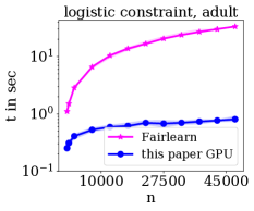
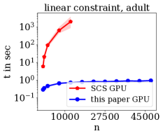
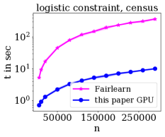
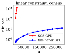
Figure 1: Running times for the logistic regression problem with fairness constraints. The two plots on the left show the running times for the adult data set and the two plots on the right for the census data set. For each data set, one plot shows the running times when the logistic loss is used in the fairness constraint and one plot when the linear loss is used.

5 Experiments

The purpose of the following experiments is to show the efficiency of our approach on a set of different classical, that is, non-deep, machine learning problems. For that purpose, we selected a number of well-known classical problems that are given as constrained optimization problems, where the optimization variables are either vectors or matrices. All these problems can also be solved on CPUs. In the supplemental material, we provide results that show that this GPU version of the GENO framework significantly outperforms the previous, efficient multi-core CPU version of the GENO framework (Laue, Mitterreiter, and Giesen 2019). Here, we compare our framework on the GPU to CVXPY paired with the cuOSQP and SCS solvers. CVXPY has a similar easy-to-use interface and also allows to solve general constrained optimization problems. Note however, that CVXPY is restricted to convex problems and cuOSQP to convex quadratic problems. It was shown that cuOSQP outperforms its CPU version OSQP by about a factor of ten (Schubiger, Banjac, and Lygeros 2020). Our experiments confirm this observation.

To the best of our knowledge, pairing CVXPY with cuOSQP or SCS are the only two approaches comparable to ours. Another framework that has been released recently that can solve convex, constrained optimization problems on the GPU is cvxpylayers (Agrawal et al. 2019). However, its focus is on making the solution of the optimization problem differentiable with respect to the input parameters for which it needs to solve a slightly larger problem. Internally, it uses CVXPY combined with the SCS solver in GPU-mode. Hence, this framework is slower than the original combination of CVXPY and SCS.

In all our experiments we made sure that the solvers that were generated by our framework always computed a solution that was better than the solution computed by the competitors in terms of objective function value and constraint satisfaction. All experiments were run on a machine equipped with an Intel i9-10980XE 18-core processor running Ubuntu 20.04.1 LTS with 128 GB of RAM, and a Quadro RTX 4000 GPU that has 8 GB of GDDR6 SDRAM and 2304 CUDA cores. Our framework took always less than 10 milliseconds for generating a solver from its mathematical description.

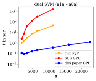
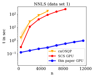
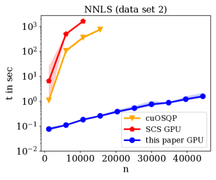
Figure 2: The plot on the left shows the running times for the SVM problem on the adult data set. The plot in the middle and the plot on the right show the running times for the non-negative least squares problem when run on the first and second data set, respectively.

Solver				Data sets
	cod-rna	covtype	ijcnn1	mushrooms	phishing	a9a	w8a
this paper GPU	0.6	0.1	1.8	0.1	1.6	0.3	1.4
cuOSQP	55.7	failed	206.5	22.0	163.5	32.8	36.1
SCS GPU	2342.0	31.3	N/A	7994.9	N/A	1094.0	1227.1

Table 1: Running times in seconds for the dual SVM problem. All data sets were subsampled to $10,000$ data points due time and memory requirements of the cuOSQP and SCS solver. N/A indicates that the solver did not finish within $10,000$ seconds.

5.1 Fairness in Machine Learning

In classical machine learning approaches, one usually minimizes a regularized empirical risk in order to make correct predictions on unseen data. However, due to various causes, e.g., bias in the data, it can happen that some group of the input data is favored over another group. Such favors can be mitigated by the introduction of constraints that explicitly prevent them. This is the goal of fairness in machine learning which has gained considerable attention over the last few years. Here, we consider fairness for binary classification.

There are a number of different fairness definitions (Agarwal et al. 2018; Barocas, Hardt, and Narayanan 2019; Donini et al. 2018), see the Fairlearn project (Bird et al. 2020, 2021) for an introduction and overview. Here, we follow the exposition and formulation in (Donini et al. 2018). Let $D=\{(x^{1},y^{1}),\ldots,(x^{m},y^{m})\}$ be a labeled data set and $A$ and $B$ be two groups, i.e., subsets of the data set. Then, one seeks to find a classifier that is statistically independent of the group membership $A$ and $B$. Depending on the type of groups $A$ and $B$, respectively, different types of fairness constraints are obtained. Since statistical independence is defined with respect to the true data distribution, which is typically unknown, one replaces the expectation over the true distribution by the empirical risk. Hence, one solves the following constrained optimization problem

$$\min_{f}\>\widehat{L}_{D}(f)+\lambda\cdot r(f)\\ \quad\operatorname{s.t.}\quad\widehat{L}_{A}(f)=\widehat{L}_{B}(f),$$

where $f\colon X\to\mathbb{R}$ is a function or model, $l\colon\mathbb{R}\times Y\to\mathbb{R}$ is a loss function, $\widehat{L}_{D}(f)=\frac{1}{|D|}\sum_{(x^{i},y^{i})\in D}l(f(x^{i}),y^{i})$ is the empirical risk of $f$ over the data set $D$, and $r(\cdot)$ is the regularizer.

Ideally, one would like to use the same loss function for the risk minimization $\widehat{L}_{D}(f)$ as in the fairness constraint $\widehat{L}_{A}(f)=\widehat{L}_{B}(f)$. The logistic loss is often used for classification. However, when the logistic loss is used in the fairness constraint, the problem becomes non-convex, even for a linear classifier. Using our framework, we can still solve this problem. However, we cannot compare its performance to cuOSQP or SCS since they only allow to solve convex problems. Thus, we compare it to the exponentiated gradient approach (Agarwal et al. 2018) paired with the Liblinear solver (Fan et al. 2008). Note, that this approach does not run on the GPU. However, to provide a better global picture, we still include it here. Only when the loss function in the fairness constraint is linear as in (Donini et al. 2018; Zemel et al. 2013), the problem becomes convex. We also consider this case and compare it to SCS. Note, the problem cannot be solved by cuOSQP since it contains exponential cones.

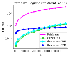
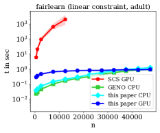
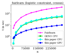
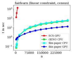
Figure 4: Running times for the logistic regression problem with fairness constraints. The two plots on the left show the running times for the adult data set and the two plots on the right for the census data set. For each data set, one plot shows the running times for using the logistic loss in the fairness constraint and one plot for using the linear loss.

We used the same setup, the same data sets, and the same preprocessing as described in the Fairlearn package (Bird et al. 2020). We used the adult data set ($48,842$ data points with $120$ features) and the census-income data set ($299,285$ data points with $400$ features) each with ‘female’ and ‘male’ as the two subgroups. For each experiment, we sampled $m$ data points from the full data set. Figure 4 shows the running times. Our framework provides similar results in terms of quality as the exponentiated gradient approach, when the logistic loss is used in the fairness constraint, and it is orders of magnitude faster than SCS on the GPU, when the linear loss is used in the fairness constraint.

5.2 Dual SVM

Support vector machines (SVMs) are a classical yet still relevant classification method. When combined with a kernel, they are usually solved in the dual problem formulation, which reads as

$$\min_{a}\,\frac{1}{2}(a\odot y)^{\top}K(a\odot y)-\|a\|_{1}\,\operatorname{s.t.}\,y^{\top}a=0,0\leq a\leq c,$$

where $K\in\mathbb{R}^{n\times n}$ is a positive semidefinite kernel matrix, $y\in\{-1,+1\}^{n}$ are the corresponding binary labels, $a\in\mathbb{R}^{n}$ are the dual variables, $\odot$ is the element-wise multiplication, and $c\in\mathbb{R}_{+}$ is the regularization parameter.

We used all data sets from the LibSVM data sets website (Lin and Fan 2021) that had more than $8000$ data points with fewer than $1000$ features such that a kernel approach is reasonable. We applied a standard Gaussian kernel with bandwidth parameter $\gamma=1$ and regularization parameter $c=1$. Table 7 shows the running times for the data sets when subsampled to $10,000$ data points. Figure 2 shows the running times for an increasing number of data points based on the original subsampled adult data set (Lin and Fan 2021). It can be seen that our approach outperforms cuOSQP as well as SCS by several orders of magnitude. The cuOSQP solver ran out of memory for problems with more than $10,000$ data points. While there is a specialized solver for solving these SVM problems on the GPU (Wen et al. 2018), the focus here is on general purpose frameworks.

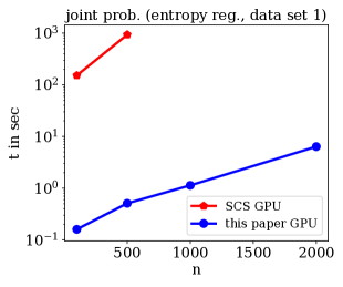
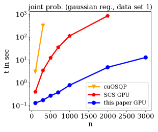
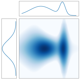
Figure 3: Running times for computing the joint probability distribution from two marginal distributions. The left plot shows the running times when the entropy prior is used and the plot in the middle when a Gaussian prior is used. The right figure visualizes the probabilities.

5.3 Non-negative Least Squares

Non-negative least squares is an extension of the least squares regression problem that requires the output to be non-negative. See (Slawski 2013) for an overview on the non-negative least squares problem. It is given as the following optimization problem

$$\min_{x}\,\left\|Ax-b\right\|_{2}^{2}\quad\operatorname{s.t.}\quad x\geq 0,$$

where $A\in\mathbb{R}^{m\times n}$ is the design matrix and $b\in\mathbb{R}^{m}$ the response vector. We ran two sets of experiments, similarly to the comparisons in (Slawski 2013), where it was shown that different algorithms behave quite differently on these problems. For experiment (i), we generated a random data matrix $A\in\mathbb{R}^{2000\times 6000}$, where the entries of $A$ were sampled uniformly at random from the unit interval and a sparse vector $x\in\mathbb{R}^{6000}$ with non-zero entries sampled from the standard Gaussian distribution and a sparsity of $0.01$. The response variables were then generated as $y=\sqrt{0.003}\cdot Ax+0.003\cdot z$, where $z\sim{\cal{N}}(0,1)$. For experiment (ii), $A\in\mathbb{R}^{6000\times 3000}$ was drawn from a Gaussian distribution and $x$ had a sparsity of $0.1$. The response variable was generated as $y=\sqrt{1/6000}\cdot Ax+0.003\cdot z$, where $z\sim{\cal{N}}(0,1)$. The differences between the two experiments are: (1) The Gram matrix $A^{\top}A$ is singular in experiment (i) and regular in experiment (ii), (2) the design matrix $A$ has isotropic rows in experiment (ii) but not in experiment (i), and (3) $x$ is significantly sparser in (i) than in (ii). To evaluate the runtime behavior for increasing problem size, we scaled the problem sizes to $A\in\mathbb{R}^{2000t\times 6000t}$ in the first experiment and to $A\in\mathbb{R}^{6000t\times 3000t}$ in the second experiment for a parameter $t\in[0,6]$. For each problem instance we performed ten runs and report the average running time along with the standard deviation in Figure 2. We stopped including SCS and cuOSQP into the experiments once their running time exceeded $1000$ seconds. It can be seen that SCS is faster than cuOSQP on the first set of experiments and slower than cuOSQP on the second set. However, our approach outperforms SCS and cuOSQP by several orders of magnitude in both sets of experiments.

5.4 Joint Probability Distribution

Given two discrete probability distributions $u\in\mathbb{R}^{m}$ and $v\in\mathbb{R}^{n}$, we are interested in their joint probability distribution $P\in\mathbb{R}^{m\times n}$. This problem has been studied intensively before, see, e.g., (Cuturi 2013; Frogner and Poggio 2019; Muzellec et al. 2017). With additional knowledge, it can be reduced to a regularized optimal transport problem. Many different regularizers have been used, for instance, an entropy, a Gaussian, or more generally, a Tsallis regularizer. The corresponding optimization problem is the following constrained optimization problem over positive matrices

$$\min_{P}\>\langle{M},{P}\rangle+\lambda\cdot r(P)\quad\operatorname{s.t.}\quad P\cdot\bm{1}=u,\,P^{\top}\cdot\bm{1}=v,\,0\leq P,$$

where $M\in\mathbb{R}^{m\times n}$ is the cost matrix, $r(.)$ is the regularizer, $\bm{1}$ is the all-ones vector, and $\lambda\in\mathbb{R}_{+}$ is the regularization parameter. In our experiments we used the entropy and the Gaussian regularizer that are both special cases of the Tsallis regularizer. In the special case that the regularizer is the entropy, $m=n$, and the cost matrix $M$ is a metric, (Cuturi 2013) showed that the problem can be solved using Sinkhorn’s algorithm (Knopp and Sinkhorn 1967). Similar results are known for other special cases (Janati et al. 2020). However, in general Sinkhorn’s algorithm cannot be used as it is the case in the present experiments, since the cost matrix is not a metric.

Here, we used synthetic data sets since the real-world data sets that are usually used for this task are very small, typically $m,n\leq 20$. We created two sets of synthetic data sets. For the first set of data sets, we let a Gaussian and a mixture of two Gaussians be the marginals, see Figure 7. Then, we discretized both distributions to obtain the marginal vectors $u$ and $v$. In this case, we set $m=n$. Hence, when $n=1000$, the corresponding optimization problem has $10^{6}$ optimization variables with lower bound constraints and $2000$ equality constraints. The cost matrix $M$ was fixed to be the discretized version $uu^{\top}$ of a two-dimensional Gaussian, and the regularization parameter was set as $\lambda=\frac{1}{2}$. We ran two sets of experiments on this data set, one where $r(.)$ is the entropy regularizer and another one with the Gaussian regularizer. Figure 7 shows the running times for both experiments for varying problem sizes. It can be seen that our approach outperforms cuOSQP and SCS by several orders of magnitude. The cuOSQP solver ran out of memory already on very small problems. The second data set was created as in (Frogner and Poggio 2019). On this data set, the speedup over cuOSQP and SCS is even more pronounced. Detailed results can be found in the appendix.

6 Conclusion

We presented an approach for solving constrained optimization problems on the GPU efficiently and included this approach into the GENO framework. The framework allows to specify a constrained optimization problem in an easy-to-read modeling language and then generates solvers in portable Python code that outperform competing state-of-the-art approaches on the GPU by several orders of magnitude. Using GPUs also for classical, that is, non-deep, machine learning becomes increasingly important as hardware vendors started to combine CPUs and GPUs on a single chip like Apple’s M1 chip.

Appendix A Appendix

In this supplementary material, we provide more details on the original L-BFGS-B algorithm, missing algorithmic details of our approach, and more experiments. The focus of the main paper is to provide an efficient algorithmic framework for solving constrained optimization problems on the GPU. However, to provide a better overall picture, we also provide comparisons for a CPU version of our approach. We compare the CPU version of our approach to its GPU version and also to the original GENO framework (Laue, Mitterreiter, and Giesen 2019), which specifically targets CPUs. Comparing running times across CPUs and GPUs is not always fair, since computations on different hardware cannot be directly compared. In order to ensure approximately fair comparisons, we used a CPU and a GPU that cost about the same. Namely, we used an Intel i9-10980XE 18-core CPU and a Quadro RTX 4000 GPU with 2304 CUDA cores.

Appendix B Comparison to Original L-BFGS-B on the GPU

In this section, we further discuss the algorithmic shortcomings of the original L-BFGS-B when ported to the GPU and provide further technical details, as already mentioned in the introduction of the main paper.

The original L-BFGS-B algorithm, like any other quasi-Newton method, approximates the function to be minimized by a quadratic model. In each iteration, the algorithm first computes the set of fixed variables, i.e., the optimization variables that are on their bounds. This is achieved as follows: The quadratic model is minimized along the path which starts at the current iterate and points into the direction of the gradient. There are two possibilities: Either the minimum is attained at the current path segment or the path first hits the boundary of the feasible region. In the first case, the minimum along the projected gradient path is found. This point is called the Cauchy point. In the second case, the path is projected back onto the feasible region and the minimization along the projected path continues. Pseudo-code and explicit formulas can be found in (Byrd et al. 1995). The main observation is that computing the minimum of the quadratic approximation along a ray only needs a few scalar operations. Whenever the path hits the boundary, the ray changes direction and the minimum along this new ray needs to be computed. This loop is repeated until the minimum is found. The total number of iterations of this loop is usually roughly of the order of the number of variables. This is an inherent sequential part that cannot benefit from parallelization. While this loop is executed on the CPU as well as on the GPU only on one core, its running time increases drastically on the GPU since its cores are much weaker. This problem is reflected in experiments and it was the main reason for designing our new algorithm.

Consider for instance the non-negative least squares problem, as described in the experiments section of the main paper. The absolute error of $10^{-10}$ was similar for both solvers and the number of iterations (between 30-40) was identical for both solvers on each data set. As can be seen from the results in Table 2 the original L-BFGS-B algorithm even slows down on the GPU. The reason is the bottleneck of the Cauchy point computation. Our approach does not suffer from the problem and parallelizes nicely on the GPU.

problem size	6000		8000		10,000		12,000
	total time	CP time	total time	CP time	total time	CP time	total time	CP time
L-BFGS-B CPU	1.5	0.3	2.6	0.4	3.6	0.5	4.9	0.6
L-BFGS-B GPU	2.8	2.5	3.5	3.1	4.1	3.6	5.2	4.6
this paper GPU	0.3		0.4		0.5		0.8

Table 2: Detailed running time comparison: depicted is the total running time in seconds as well as the time in seconds spent for the Cauchy point computation (CP) for the non-negative least squares problem for varying problem sizes. Larger problem sizes do not fit into the GPU RAM anymore.

Appendix C Missing Algorithmic Details

Here, we provide details for the two-loop algorithm and the augmented Lagrangian algorithm.

C.1 Modified Two-loop Recursion

In general, the purpose of the two-loop recursion algorithm (Nocedal and Wright 1999) is to solve the quasi-Newton equation for computing the new search direction $d^{k}$, i.e.,

$$-\nabla f(x^{k})=B^{k}d^{k},$$

where $B^{k}$ is the Hessian approximation in iteration $k$. Since some of the variables are fixed in iteration $k$, the equation needs to be solved only for the subset $S^{k}$ of free variables, i.e.,

$$-\nabla f(x^{k})[S^{k}]=B^{k}[S^{k},S^{k}]d^{k}[S^{k}].$$

The new search direction that is computed by the L-BFGS update rule needs to be a descent direction. In order to satisfy this constraint, the Hessian approximation $B^{k}$ needs to be positive definite. In general, if each correction pair $(y^{i},s^{i})$ satisfies the curvature condition $\langle{y^{i}},{s^{i}}\rangle\geq\varepsilon\|y^{i}\|^{2}$, then $B^{k}$ has a smallest eigenvalue that can be bounded by a positive constant $c$, see (Mokhtari and Ribeiro 2015). Even when the objective function is convex and the curvature condition is satisfied for all $i\leq k$, it can happen that the curvature condition is violated on the subspace of the free variables with indices in $S^{k}$, i.e., it can even happen that $\langle{y^{i}[S^{k}]},{s^{i}[S^{k}]}\rangle<0$. Using this correction pair for computing the next search direction, does not provide a descent direction. Hence, in order for the method to work, the corresponding curvature condition needs to be checked for all stored curvature pairs and the current index set $S^{k}$. Algorithm 3 incorporates this strategy.

As mentioned in the main paper, the strong Wolfe conditions in the line search assure that the curvature condition is satisfied for the whole correction pair $(y^{i},s^{i})$. However, since this does not imply the curvature condition for the reduced correction pair $(y^{i}[S^{k}],s^{i}[S^{k}])$, it is not necessary to satisfy the strong Wolfe conditions. Instead, the weaker Armijo conditions are sufficient in the line search. The Armijo conditions are often satisfied after fewer steps in the line search.

Algorithm 3 Modified Two-loop Recursion

1: Input: gradient $\nabla f(x^{k})$, index set $S^{k}$

2:$q=\nabla f(x^{k})[S^{k}]$

3:for $i=k-1,\ldots,k-m$ do

4:   $\rho^{i}=\langle{s^{i}[S^{k}]},{y^{i}[S^{k}]}\rangle$

5:   if $\rho^{i}>\varepsilon\|y^{i}\|^{2}$ then

6:      $\alpha^{i}=\frac{1}{\rho^{i}}\cdot\langle{s^{i}[S^{k}]},{q}\rangle$

7:      $q=q-\alpha^{i}\cdot y^{i}[S^{k}]$

8:   end if

9:end for

10:if $\rho^{k-1}>\varepsilon\|y^{k-1}\|^{2}$ then

11:   $q=\frac{\rho^{k-1}}{\|y^{k-1}\|^{2}}\cdot q$

12:end if

13:for $i=k-m,\ldots,k-1$ do

14:   if $\rho^{i}>\varepsilon\|y^{i}\|^{2}$ then

15:      $\beta=\frac{1}{\rho^{i}}\cdot\langle{y^{i}[S^{k}]},{q}\rangle$

16:      $q=q+(\alpha^{i}-\beta)\cdot s^{i}[S^{k}]$

17:   end if

18:end for

19:return q

C.2 Augmented Lagrangian Algorithm

The presented algorithm can solve optimization problems with box constraints, i.e., upper and lower bounds on the variables. In order to solve general constrained optimization problems, i.e.,

$$\begin{array}[]{rl}\displaystyle\min_{x}&f(x)\\ \operatorname{s.t.}&h(x)=0\\ &g(x)\leq 0\\ &l\leq x\leq u,\end{array}$$ (5)

we use the augmented Lagrangian algorithm. It reduces the constrained optimization problem to a sequence of box-constrained optimization problems by incorporating the constraints into the augmented Lagrangian of the problem, i.e.,

$$L(x,\lambda,\mu,\rho)=f(x)+\frac{\rho}{2}\left\|h(x)+\lambda/\rho\right\|^{2}+\frac{\rho}{2}\left\|\left(g(x)+\mu/\rho\right)_{+}\right\|^{2},$$ (6)

where $\lambda\in\mathbb{R}^{m}$ and $\mu\in\mathbb{R}_{\geq 0}^{p}$ are Lagrange multipliers, $\rho>0$ is a constant, and $(v)_{+}$ denotes $\max\{v,0\}$.

The augmented Lagrangian algorithm is shown in Algorithm 4. It runs in iterations and minimizes the augmented Lagrangian function (6) in each iteration using Algorithm 1. Then, it updates the Lagrangian multipliers $\lambda$ and $\mu$. If the infinity norm of the constraint violation is not halved in an iteration, then $\rho$ is multiplied by a factor of 2. Convergence of the augmented Lagrangian algorithm was shown in (Bertsekas 1999; Birgin and Martínez 2014).

Algorithm 4 Augmented Lagrangian Algorithm

1:input: constrained optimization Problem (5)

2:output: approximate solution $x\in\mathbb{R}^{n},\lambda\in\mathbb{R}^{p},\mu\in\mathbb{R}_{\geq 0}^{m}$

3:initialize $x^{0}=0$, $\lambda^{0}=0$, $\mu^{0}=0$, and $\rho=1$

4:repeat

5:   $x^{k+1}:=\quad\operatorname{argmin}_{l\leq x\leq u}\,L(x,\lambda^{k},\mu^{k},\rho)$

6:   $\lambda^{k+1}:=\quad\lambda^{k}+\rho h(x^{k+1})$

7:   $\mu^{k+1}:=\quad\left(\mu^{k}+\rho g(x^{k+1})\right)_{+}$

8:   update $\rho$

9:until convergence

10:return $x^{k},\lambda^{k},\mu^{k}$

Appendix D Experiments

Here, we present the comparisons of our framework including its CPU version and the GENO framework (Laue, Mitterreiter, and Giesen 2019) for CPUs. We also include the running times for the joint probability experiment on the second data set that was excluded from the main paper due to space constraints. It can be seen that our framework on the GPU outperforms the highly efficient GENO framework by a large margin. Since the solvers generated by our framework are written entirely in Python, they can also run on the CPU by mapping all linear algebra expressions to NumPy instead of CuPy. This allows to run our framework also on the CPU. The corresponding entry in the tables is ‘this paper CPU’. In all experiments, it can be seen that the GPU version of our framework outperforms all other frameworks once the size of the data set is reasonably large. For small data sets, the full capabilities of the GPU cannot be exploited, and hence, it does not pay off to run them on the GPU. Note again, the generated solvers of our approach were run until they obtained a smaller objective function value and constraint violation than the competing approaches. The absolute errors were usually between $10^{-3}$ and $10^{-5}$.

D.1 Fairness in Machine Learning

Solver	fairlearn (logistic constraint, adult)
	500	2500	12500	22500	32500	42500
this paper GPU	$0.3\pm 0.0$	$0.4\pm 0.0$	$0.6\pm 0.0$	$0.7\pm 0.0$	$0.7\pm 0.0$	$0.8\pm 0.0$
this paper CPU	$0.0\pm 0.0$	$0.1\pm 0.0$	$0.3\pm 0.0$	$0.6\pm 0.0$	$1.0\pm 0.1$	$1.4\pm 0.1$
GENO CPU	$0.0\pm 0.0$	$0.1\pm 0.0$	$0.2\pm 0.0$	$0.5\pm 0.0$	$0.8\pm 0.0$	$1.3\pm 0.1$
Fairlearn	$1.1\pm 0.1$	$2.9\pm 0.0$	$10.4\pm 0.7$	$16.7\pm 1.0$	$23.8\pm 1.4$	$30.0\pm 0.2$

Table 3: Running times in seconds for fairlearn (logistic constraint, adult).

Solver	fairlearn (linear constraint, adult)
	500	2500	12500	22500	32500	42500
this paper GPU	$0.3\pm 0.0$	$0.5\pm 0.0$	$0.7\pm 0.0$	$0.8\pm 0.1$	$0.9\pm 0.1$	$0.9\pm 0.1$
this paper CPU	$0.0\pm 0.0$	$0.1\pm 0.0$	$0.2\pm 0.0$	$0.4\pm 0.0$	$0.8\pm 0.1$	$1.1\pm 0.1$
GENO CPU	$0.0\pm 0.0$	$0.0\pm 0.0$	$0.2\pm 0.0$	$0.3\pm 0.0$	$0.6\pm 0.0$	$0.9\pm 0.0$
SCS GPU	$6.1\pm 0.8$	$95.5\pm 17.9$	$2056.8\pm 971.6$	N/A	N/A	N/A

Table 4: Running times in seconds for fairlearn (linear constraint, adult).

Solver	fairlearn (logistic constraint, census)
	10000	50000	110000	170000	230000	290000
this paper GPU	$0.9\pm 0.1$	$2.3\pm 0.1$	$4.3\pm 0.1$	$6.1\pm 0.4$	$8.0\pm 0.3$	$10.1\pm 0.3$
this paper CPU	$0.9\pm 0.1$	$8.5\pm 0.5$	$22.0\pm 0.9$	$35.3\pm 1.3$	$48.7\pm 1.6$	$61.7\pm 3.3$
GENO CPU	$0.8\pm 0.0$	$7.6\pm 0.4$	$18.7\pm 0.9$	$31.6\pm 2.0$	$43.3\pm 2.0$	$52.9\pm 2.8$
Fairlearn	$9.4\pm 1.0$	$45.5\pm 2.8$	$120.0\pm 7.5$	$199.7\pm 17.6$	$281.9\pm 11.9$	$366.6\pm 16.0$

Table 5: Running times in seconds for fairlearn (logistic constraint, census).

Solver	fairlearn (linear constraint, census)
	2500	10000	50000	170000	230000	290000
this paper GPU	$0.6\pm 0.0$	$0.9\pm 0.1$	$2.2\pm 0.2$	$7.6\pm 0.7$	$10.6\pm 0.3$	$13.4\pm 1.4$
this paper CPU	$0.1\pm 0.0$	$0.7\pm 0.0$	$5.8\pm 0.6$	$32.0\pm 2.9$	$47.8\pm 4.5$	$64.2\pm 5.7$
GENO CPU	$0.1\pm 0.0$	$0.6\pm 0.0$	$5.4\pm 0.7$	$27.4\pm 3.0$	$39.9\pm 3.1$	$54.8\pm 7.3$
SCS GPU	$129.3\pm 18.6$	$1331.3\pm 146.7$	N/A	N/A	N/A	N/A

Table 6: Running times in seconds for fairlearn (linear constraint, census).

D.2 Support Vector Machines

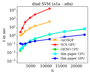
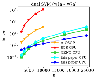
Figure 5: The plot on the left shows the running times for the SVM problem on the adult data set for an increasing number of data points. The plot on the right shows the web data set for an increasing number of data points.

Solver	Data sets
	cod-rna	covtype	ijcnn1	mushrooms	phishing	a9a	w8a
this paper GPU	0.7	0.1	1.8	0.1	1.7	0.3	1.5
this paper CPU	2.0	0.4	5.4	0.3	5.4	1.1	4.3
GENO CPU	1.9	0.4	19.4	0.4	6.4	1.0	3.2
cuOSQP	55.7	failed	206.6	22.1	163.6	32.9	36.1
SCS GPU	2342.1	31.4	N/A	7995.0	N/A	1094.1	1227.1

Table 7: Running times in seconds for the dual SVM problem. All data sets were subsampled to $10,000$ data points. N/A indicates that the solver did not finish within $10,000$ seconds.

Solver	dual SVM (a1a – a8a)
	1605	2265	3185	4781	6414	11220	16100	22696
this paper GPU	$0.1$	$0.1$	$0.1$	$0.2$	$0.2$	$0.4$	$0.7$	$1.3$
this paper CPU	$0.0$	$0.0$	$0.1$	$0.3$	$0.5$	$1.5$	$3.2$	$6.6$
GENO CPU	$0.0$	$0.0$	$0.1$	$0.2$	$0.4$	$1.4$	$3.0$	$5.8$
cuOSQP	$1.0$	$1.5$	$3.0$	$7.1$	$13.5$	$42.9$	N/A	N/A
SCS GPU	$2.6$	$7.7$	$40.0$	$127.3$	$312.9$	$1565.9$	N/A	N/A

Table 8: Running times in seconds for dual SVM (adult data set, a1a – a8a).

Solver	dual SVM (w1a – w7a)
	2477	3470	4912	7366	9888	17188	24692
this paper GPU	$0.4$	$0.6$	$0.7$	$1.1$	$1.5$	$3.5$	$7.0$
this paper CPU	$0.2$	$0.3$	$0.8$	$2.0$	$4.1$	$13.6$	$37.0$
GENO CPU	$0.1$	$0.2$	$0.5$	$1.5$	$2.6$	$8.5$	$22.4$
cuOSQP	$1.8$	$3.5$	$7.4$	$19.8$	$35.3$	N/A	N/A
SCS GPU	$14.9$	$49.7$	$147.9$	$493.1$	$1159.0$	N/A	N/A

Table 9: Running times in seconds for dual SVM (web data set, w1a – w7a).

D.3 Non-negative Least Squares

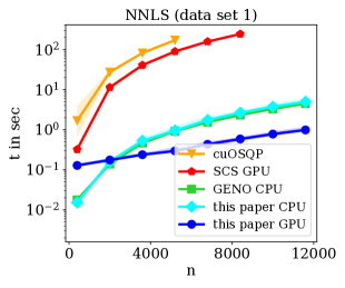
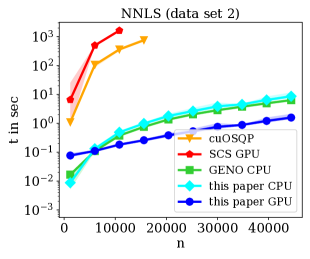
Figure 6: The plots show the running times for the non-negative least squares problem when run on the first and second data set.

Solver	NNLS (data set 1)
	3600	5200	6800	8400	10000	11600
this paper GPU	$0.2\pm 0.0$	$0.3\pm 0.0$	$0.4\pm 0.0$	$0.6\pm 0.0$	$0.8\pm 0.1$	$1.0\pm 0.1$
this paper CPU	$0.5\pm 0.1$	$1.0\pm 0.1$	$1.7\pm 0.2$	$2.6\pm 0.2$	$3.7\pm 0.4$	$5.0\pm 0.5$
GENO CPU	$0.5\pm 0.0$	$0.9\pm 0.0$	$1.5\pm 0.0$	$2.3\pm 0.0$	$3.3\pm 0.1$	$4.5\pm 0.1$
cuOSQP	$82.0\pm 1.0$	$171.4\pm 5.5$	N/A	N/A	N/A	N/A
SCS GPU	$40.7\pm 0.4$	$89.5\pm 1.0$	$157.7\pm 2.0$	$243.4\pm 3.3$	N/A	N/A

Table 10: Running times in seconds for NNLS (data set 1).

Solver	NNLS (data set 2)
	6000	10800	15600	25200	34800	44400
this paper GPU	$0.1\pm 0.0$	$0.2\pm 0.0$	$0.3\pm 0.0$	$0.5\pm 0.1$	$0.9\pm 0.0$	$1.6\pm 0.2$
this paper CPU	$0.1\pm 0.0$	$0.5\pm 0.0$	$1.0\pm 0.1$	$2.7\pm 0.4$	$4.5\pm 0.1$	$8.6\pm 1.3$
GENO CPU	$0.1\pm 0.0$	$0.4\pm 0.0$	$0.8\pm 0.0$	$2.1\pm 0.0$	$3.8\pm 0.0$	$6.4\pm 0.1$
cuOSQP	$106.3\pm 10.5$	$362.3\pm 27.7$	$755.4\pm 41.1$	N/A	N/A	N/A
SCS GPU	$500.2\pm 4.2$	$1637.4\pm 14.3$	N/A	N/A	N/A	N/A

Table 11: Running times in seconds for NNLS (data set 2).

D.4 Joint Probability

Here, we show the running times for computing the joint probability distribution of two probability distributions, i.e., a distribution that has the two given distributions as marginals, see also the main paper. The second data set was created in the same way as in (Frogner and Poggio 2019), i.e., we sampled $u$ and $v$ uniformly at random from the unit interval and scaled them such that each vector sums up to one. All entries of the cost matrices $M$ were also sampled uniformly at random from the unit interval. We fixed the regularization parameter $\lambda=\frac{1}{2}$. We set the size of the problems to be $m=2n$. Hence, when $n=1000$, the corresponding optimization problem involves $2\cdot 10^{6}$ optimization variables and has $3000$ constraints. Figure 7 shows the running times for both data sets and both regularizers for varying problem sizes, including the running times for the CPU versions.

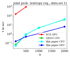
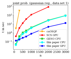
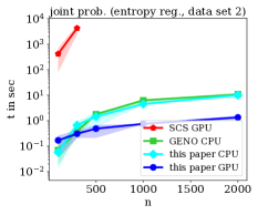
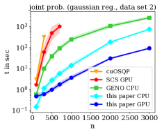
Figure 7: Running times for computing a joint probability distribution from two marginal distributions. The two plots on the left show the running times for the first data set and the two plots on the right the running times for the second data set. For each data set, we show the running times when the entropy prior is used and when the Gaussian prior is used. Note, that the cuOSQP solver cannot solve the problem when the entropy prior is used. Since the second data set is drawn from a random distribution, we ran all solvers ten times and report the mean running time and corresponding error bars.

Solver	joint prob. (entropy reg., data set 1)
	100	500	1000	2000
this paper GPU	$0.2$	$0.5$	$1.1$	$6.4$
this paper CPU	$0.1$	$0.9$	$4.6$	$41.2$
GENO CPU	$0.1$	$0.9$	$4.8$	$38.5$
SCS GPU	$151.8$	$933.5$	N/A	N/A

Table 12: Running times in seconds for joint prob. (entropy reg., data set 1).

Solver	joint prob. (gaussian reg., data set 1)
	100	300	500	700	1000	2000	3000
this paper GPU	$0.1$	$0.2$	$0.3$	$0.4$	$0.8$	$4.8$	$13.0$
this paper CPU	$0.0$	$0.2$	$0.8$	$1.2$	$3.6$	$25.1$	$86.2$
GENO CPU	$0.1$	$0.4$	$1.1$	$1.8$	$4.1$	$27.7$	$90.9$
cuOSQP	$3.1$	$318.8$	N/A	N/A	N/A	N/A	N/A
SCS GPU	$0.4$	$3.5$	$12.5$	$36.0$	$114.1$	$861.4$	N/A

Table 13: Running times in seconds for joint prob. (gaussian reg., data set 1).

Solver	joint prob. (entropy reg., data set 2)
	100	300	500	1000	2000
this paper GPU	$0.2\pm 0.1$	$0.3\pm 0.1$	$0.5\pm 0.2$	$0.7\pm 0.0$	$1.3\pm 0.2$
this paper CPU	$0.1\pm 0.0$	$0.7\pm 0.1$	$1.4\pm 0.6$	$4.5\pm 0.0$	$10.1\pm 1.5$
GENO CPU	$0.1\pm 0.0$	$0.4\pm 0.2$	$1.8\pm 0.0$	$6.3\pm 0.9$	$10.8\pm 0.0$
SCS GPU	$417.9\pm 257.7$	$4267.7\pm 1408.3$	N/A	N/A	N/A

Table 14: Running times in seconds for joint prob. (entropy reg., data set 2).

Solver	joint prob. (gaussian reg., data set 2)
	300	700	1000	2000	3000
this paper GPU	$0.6\pm 0.1$	$1.7\pm 0.3$	$3.6\pm 0.6$	$30.2\pm 1.5$	$92.3\pm 1.9$
this paper CPU	$1.1\pm 0.2$	$5.7\pm 1.0$	$13.9\pm 2.3$	$182.9\pm 9.1$	$746.1\pm 21.9$
GENO CPU	$9.9\pm 0.6$	$92.2\pm 13.2$	$240.1\pm 35.3$	$1068.0\pm 153.7$	$2622.4\pm 236.7$
cuOSQP	$314.0\pm 7.8$	N/A	N/A	N/A	N/A
SCS GPU	$60.4\pm 39.4$	$1009.3\pm 355.1$	N/A	N/A	N/A

Table 15: Running times in seconds for joint prob. (gaussian reg., data set 2).

References

- Agarwal et al. (2018) Agarwal, A.; Beygelzimer, A.; Dudík, M.; Langford, J.; and Wallach, H. M. 2018. A Reductions Approach to Fair Classification. In International Conference on Machine Learning, (ICML), 60–69.
- Agrawal et al. (2019) Agrawal, A.; Amos, B.; Barratt, S. T.; Boyd, S. P.; Diamond, S.; and Kolter, J. Z. 2019. Differentiable Convex Optimization Layers. In Advances in Neural Information Processing Systems (NeurIPS), 9558–9570.
- Agrawal et al. (2018) Agrawal, A.; Verschueren, R.; Diamond, S.; and Boyd, S. 2018. A rewriting system for convex optimization problems. Journal of Control and Decision, 5(1): 42–60.
- Barocas, Hardt, and Narayanan (2019) Barocas, S.; Hardt, M.; and Narayanan, A. 2019. Fairness and Machine Learning. http://www.fairmlbook.org. Accessed: 2022-02-22.
- Beck and Teboulle (2009) Beck, A.; and Teboulle, M. 2009. A Fast Iterative Shrinkage-Thresholding Algorithm for Linear Inverse Problems. SIAM J. Imaging Sci., 2(1): 183–202.
- Bertsekas (1982) Bertsekas, D. P. 1982. Projected Newton Methods for Optimization Problems with Simple Constraints. SIAM Journal on Control and Optimization, 20(2): 221–246.
- Bertsekas (1999) Bertsekas, D. P. 1999. Nonlinear Programming. Belmont, MA: Athena Scientific.
- Bird et al. (2020) Bird, S.; Dudík, M.; Edgar, R.; Horn, B.; Lutz, R.; Milan, V.; Sameki, M.; Wallach, H.; and Walker, K. 2020. Fairlearn: A toolkit for assessing and improving fairness in AI. Technical Report MSR-TR-2020-32, Microsoft.
- Bird et al. (2021) Bird, S.; Dudík, M.; Edgar, R.; Horn, B.; Lutz, R.; Milan, V.; Sameki, M.; Wallach, H.; and Walker, K. 2021. Fairlearn – Improve fairness of AI systems. https://www.fairlearn.org. Accessed: 2022-02-22.
- Birgin and Martínez (2014) Birgin, E. G.; and Martínez, J. M. 2014. Practical augmented Lagrangian methods for constrained optimization, volume 10 of Fundamentals of Algorithms. SIAM.
- Boyd et al. (2011) Boyd, S. P.; Parikh, N.; Chu, E.; Peleato, B.; and Eckstein, J. 2011. Distributed Optimization and Statistical Learning via the Alternating Direction Method of Multipliers. Foundations and Trends in Machine Learning, 3(1): 1–122.
- Byrd et al. (1995) Byrd, R. H.; Lu, P.; Nocedal, J.; and Zhu, C. 1995. A Limited Memory Algorithm for Bound Constrained Optimization. SIAM J. Scientific Computing, 16(5): 1190–1208.
- Cuturi (2013) Cuturi, M. 2013. Sinkhorn Distances: Lightspeed Computation of Optimal Transport. In Advances in Neural Information Processing Systems (NIPS), 2292–2300.
- Diamond and Boyd (2016) Diamond, S.; and Boyd, S. 2016. CVXPY: A Python-embedded modeling language for convex optimization. Journal of Machine Learning Research, 17(83): 1–5.
- Donini et al. (2018) Donini, M.; Oneto, L.; Ben-David, S.; Shawe-Taylor, J.; and Pontil, M. 2018. Empirical Risk Minimization Under Fairness Constraints. In Advances in Neural Information Processing Systems (NeurIPS), 2796–2806.
- Fan et al. (2008) Fan, R.-E.; Chang, K.-W.; Hsieh, C.-J.; Wang, X.-R.; and Lin, C.-J. 2008. LIBLINEAR: A Library for Large Linear Classification. Journal of Machine Learning Research, 9: 1871–1874.
- Frogner and Poggio (2019) Frogner, C.; and Poggio, T. A. 2019. Fast and Flexible Inference of Joint Distributions from their Marginals. In International Conference on Machine Learning, ICML, 2002–2011.
- Funke, Laue, and Storandt (2016) Funke, S.; Laue, S.; and Storandt, S. 2016. Deducing individual driving preferences for user-aware navigation. In International Conference on Advances in Geographic Information Systems, 14:1–14:9.
- Funke, Laue, and Storandt (2017) Funke, S.; Laue, S.; and Storandt, S. 2017. Personal Routes with High-Dimensional Costs and Dynamic Approximation Guarantees. In International Symposium on Experimental Algorithms, (SEA), 18:1–18:13.
- Giesen and Laue (2016) Giesen, J.; and Laue, S. 2016. Distributed Convex Optimization with Many Convex Constraints. arXiv:1610.02967.
- Glockner (2021) Glockner, G. 2021. Does Gurobi support GPUs? https://support.gurobi.com/hc/en-us/articles/360012237852-Does-Gurobi-support-GPUs. Accessed: 2021-04-26.
- Hestenes (1969) Hestenes, M. R. 1969. Multiplier and gradient methods. Journal of Optimization Theory and Applications, 4(5): 303–320.
- Janati et al. (2020) Janati, H.; Muzellec, B.; Peyré, G.; and Cuturi, M. 2020. Entropic Optimal Transport between Unbalanced Gaussian Measures has a Closed Form. In Advances in Neural Information Processing Systems (NeurIPS).
- Kim, Sra, and Dhillon (2010) Kim, D.; Sra, S.; and Dhillon, I. S. 2010. Tackling Box-Constrained Optimization via a New Projected Quasi-Newton Approach. SIAM J. Sci. Comput., 32(6): 3548–3563.
- Knopp and Sinkhorn (1967) Knopp, P.; and Sinkhorn, R. 1967. Concerning nonnegative matrices and doubly stochastic matrices. Pacific Journal of Mathematics, 21(2): 343 – 348.
- Laue, Mitterreiter, and Giesen (2018) Laue, S.; Mitterreiter, M.; and Giesen, J. 2018. Computing Higher Order Derivatives of Matrix and Tensor Expressions. In Advances in Neural Information Processing Systems (NeurIPS).
- Laue, Mitterreiter, and Giesen (2019) Laue, S.; Mitterreiter, M.; and Giesen, J. 2019. GENO – GENeric Optimization for Classical Machine Learning. In Advances in Neural Information Processing Systems (NeurIPS).
- Laue, Mitterreiter, and Giesen (2020) Laue, S.; Mitterreiter, M.; and Giesen, J. 2020. A Simple and Efficient Tensor Calculus. In Conference on Artificial Intelligence (AAAI), 4527–4534.
- Li and Lin (2015) Li, H.; and Lin, Z. 2015. Accelerated Proximal Gradient Methods for Nonconvex Programming. In Advances in Neural Information Processing Systems (NIPS), 379–387.
- Lin and Fan (2021) Lin, C.-J.; and Fan, R.-E. 2021. LIBSVM data sets. https://www.csie.ntu.edu.tw/~cjlin/libsvmtools/datasets. Accessed: 2022-02-22.
- Meng et al. (2016) Meng, X.; Bradley, J.; Yavuz, B.; Sparks, E.; Venkataraman, S.; Liu, D.; Freeman, J.; Tsai, D.; Amde, M.; Owen, S.; Xin, D.; Xin, R.; Franklin, M. J.; Zadeh, R.; Zaharia, M.; and Talwalkar, A. 2016. MLlib: Machine Learning in Apache Spark. Journal of Machine Learning Research, 17(1).
- Mokhtari and Ribeiro (2015) Mokhtari, A.; and Ribeiro, A. 2015. Global convergence of online limited memory BFGS. J. Mach. Learn. Res., 16: 3151–3181.
- Morales and Nocedal (2011) Morales, J. L.; and Nocedal, J. 2011. Remark on ”Algorithm 778: L-BFGS-B: Fortran subroutines for large-scale bound constrained optimization”. ACM Trans. Math. Softw., 38(1): 7:1–7:4.
- Muzellec et al. (2017) Muzellec, B.; Nock, R.; Patrini, G.; and Nielsen, F. 2017. Tsallis Regularized Optimal Transport and Ecological Inference. In AAAI Conference on Artificial Intelligence (AAAI), 2387–2393.
- Nesterov (1983) Nesterov, Y. 1983. A method for unconstrained convex minimization problem with the rate of convergence . Doklady AN USSR (translated as Soviet Math. Docl.), 269.
- Nesterov (2004) Nesterov, Y. E. 2004. Introductory Lectures on Convex Optimization - A Basic Course, volume 87 of Applied Optimization. Springer.
- Nocedal and Wright (1999) Nocedal, J.; and Wright, S. J. 1999. Numerical Optimization. Springer.
- O’Donoghue et al. (2016) O’Donoghue, B.; Chu, E.; Parikh, N.; and Boyd, S. 2016. Conic Optimization via Operator Splitting and Homogeneous Self-Dual Embedding. Journal of Optimization Theory and Applications, 169(3): 1042–1068.
- O’Donoghue et al. (2019) O’Donoghue, B.; Chu, E.; Parikh, N.; and Boyd, S. 2019. SCS: Splitting Conic Solver, version 2.1.3. https://github.com/cvxgrp/scs. Accessed: 2022-02-22.
- Okuta et al. (2017) Okuta, R.; Unno, Y.; Nishino, D.; Hido, S.; and Loomis, C. 2017. CuPy: A NumPy-Compatible Library for NVIDIA GPU Calculations. In Proceedings of Workshop on Machine Learning Systems (LearningSys) in The Thirty-first Annual Conference on Neural Information Processing Systems (NIPS).
- Parikh and Boyd (2014) Parikh, N.; and Boyd, S. P. 2014. Proximal Algorithms. Found. Trends Optim., 1(3): 127–239.
- Pedregosa et al. (2011) Pedregosa, F.; Varoquaux, G.; Gramfort, A.; Michel, V.; Thirion, B.; Grisel, O.; Blondel, M.; Prettenhofer, P.; Weiss, R.; Dubourg, V.; Vanderplas, J.; Passos, A.; Cournapeau, D.; Brucher, M.; Perrot, M.; and Duchesnay, E. 2011. Scikit-learn: Machine Learning in Python. Journal of Machine Learning Research, 12: 2825–2830.
- Powell (1969) Powell, M. J. D. 1969. Algorithms for nonlinear constraints that use Lagrangian functions. Mathematical Programming, 14(1): 224–248.
- Rodomanov and Nesterov (2021) Rodomanov, A.; and Nesterov, Y. E. 2021. New Results on Superlinear Convergence of Classical Quasi-Newton Methods. J. Optim. Theory Appl., 188(3): 744–769.
- Schmidt, Kim, and Sra (2011) Schmidt, M.; Kim, D.; and Sra, S. 2011. Projected Newton-type Methods in Machine Learning. In Sra, S.; Nowozin, S.; and Wright, S. J., eds., Optimization for Machine Learning, chapter 11, 305–329. MIT Press.
- Schmidt et al. (2009) Schmidt, M.; van den Berg, E.; Friedlander, M. P.; and Murphy, K. P. 2009. Optimizing Costly Functions with Simple Constraints: A Limited-Memory Projected Quasi-Newton Algorithm. In International Conference on Artificial Intelligence and Statistics, (AISTATS), 456–463.
- Schubiger, Banjac, and Lygeros (2020) Schubiger, M.; Banjac, G.; and Lygeros, J. 2020. GPU acceleration of ADMM for large-scale quadratic programming. J. Parallel Distributed Comput., 144: 55–67.
- Slawski (2013) Slawski, M. 2013. Problem-specific analysis of non-negative least squares solvers with a focus on instances with sparse solutions. https://sites.google.com/site/slawskimartin/code. Accessed: 2022-02-22.
- Stellato et al. (2020) Stellato, B.; Banjac, G.; Goulart, P.; Bemporad, A.; and Boyd, S. P. 2020. OSQP: an operator splitting solver for quadratic programs. Math. Program. Comput., 12(4): 637–672.
- van den Berg (2020) van den Berg, E. 2020. A hybrid quasi-Newton projected-gradient method with application to Lasso and basis-pursuit denoising. Math. Program. Comput., 12(1): 1–38.
- Wen et al. (2018) Wen, Z.; Shi, J.; Li, Q.; He, B.; and Chen, J. 2018. ThunderSVM: A Fast SVM Library on GPUs and CPUs. Journal of Machine Learning Research, 19(21): 1–5.
- Zaharia et al. (2016) Zaharia, M.; Xin, R. S.; Wendell, P.; Das, T.; Armbrust, M.; Dave, A.; Meng, X.; Rosen, J.; Venkataraman, S.; Franklin, M. J.; Ghodsi, A.; Gonzalez, J.; Shenker, S.; and Stoica, I. 2016. Apache Spark: a unified engine for big data processing. Commun. ACM, 59(11): 56–65.
- Zemel et al. (2013) Zemel, R. S.; Wu, Y.; Swersky, K.; Pitassi, T.; and Dwork, C. 2013. Learning Fair Representations. In International Conference on Machine Learning (ICML), 325–333.
- Zhu et al. (1997) Zhu, C.; Byrd, R. H.; Lu, P.; and Nocedal, J. 1997. Algorithm 778: L-BFGS-B: Fortran Subroutines for Large-Scale Bound-Constrained Optimization. ACM Trans. Math. Softw., 23(4): 550–560.