Theoretical analysis of surface brightness–colour relations for late-type stars using MARCS model atmospheres

Abstract

Context. Surface brightness–colour relations (SBCRs) are largely used for general studies in stellar astrophysics and for determining extragalactic distances. Based on a careful selection of stars and a homogeneous methodology, it has been recently shown that the SBCR for late-type stars depends on the spectral type and luminosity class.

Aims. Based on simulated spectra of late-type stars using MARCS model atmospheres, our aim is to analyse the effect of stellar fundamental parameters on the surface brightness. We also compare theoretical and recent empirical SBCRs.

Methods. We used MARCS model atmospheres to compute spectra and obtain the surface brightness of stars. We first explored the parameter space of MARCS (i.e. effective temperature, $\log g$, $\mathrm{[Fe/H]}$, microturbulence, and mass) in order to quantify their impact on the surface brightness. Then we considered a relation between the effective temperature and $\log g$ for late dwarfs and giants, as well as a solar metallicity, in order to allow a consistent comparison of theoretical and empirical SBCRs.

Results. We find that the SBCR is not sensitive to the microturbulence and mass. The effect of metallicity on the SBCR is found to be larger for dwarfs than for giants. It is also larger when considering larger $V-K_{s}$ values. We also find that a difference of 0.5 dex in metallicity between Galactic and LMC SBCRs does not affect the recent LMC distance determination, based on eclipsing binaries, by more than 0.4%. By comparing theoretical with empirical SBCRs, we find a good agreement of less than 2$\sigma$ for F5–K7 dwarfs and giants stars, while a larger discrepancy is found for M dwarfs and giants (about 4–6$\sigma$). The surface gravity properties, as modelled in MARCS, explain the differences in the empirical SBCRs in terms of class. We finally find that theoretical and empirical SBCRs for Cepheids are consistent.

Conclusions. Carefully considering metallicity and $\log g$ is mandatory when calibrating or using SBCRs.

1 Introduction

Surface brightness–colour relations (SBCRs) are efficient tools for easily determining stellar angular diameters from photometric measurements. In the course of the Araucaria project, Pietrzyński et al. (2019) estimated the distance to the Large Magellanic Cloud, based on 20 late-type eclipsing binaries, with a precision of 1%. This achievement could be done using a precise SBCR calibrated on 41 nearby red clump giant stars (Gallenne et al., 2018). In the same way, other works made use of giant late-type eclipsing binaries to constrain the Small Magellanic Cloud distance (Graczyk et al., 2020). To derive extragalactic distances from eclipsing binaries, the radii of the two components are estimated from the transit, by combining photometric and spectroscopic measurements. Then, the angular diameter of each component is estimated from the magnitude and colour of stars using a SBCR. Finally, the combination of radii (in kms) and angular diameters (in milliarcseconds) allows us to deduce the distance. The SBCRs should also play an important role in the context of the PLAnetary Transits and Oscillations of stars (PLATO, Catala & PLATO Team 2006) space mission, planned for launch in 2026, in order to characterise exoplanetary systems.

To date, authors have developed various SBCRs, covering all spectral types and luminosity classes. Several comparisons (Nardetto, 2018) reveal precise but inconsistent SBCRs for late-type stars (i.e. $V-K_{s}>1\,$ mag) at the 10% level, while SBCRs for early-type stars (i.e. $V-K_{s}<1\,$ mag) have recently been improved from around 7% precision Challouf et al. (2014) to 2–3% (Salsi et al., 2021). Years ago, Fouque & Gieren (1997) observed a significant difference in the SBCRs according to the luminosity class of stars. This dependance was then observed in several other studies (Boyajian et al., 2014; Challouf et al., 2014; Kervella et al., 2004c; Nardetto, 2018; van Belle, 1999). Salsi et al. (2020) (hereafter Paper I) calibrate SBCRs for late-type stars by implementing for the very first time criteria to properly select the samples, and use a homogeneous methodology in the calibration process. This allows us to clearly disentangle the SBCRs regarding their domain of spectral types (FGK and M stars) and luminosity classes. In Salsi et al. (2021) (hereafter Paper II), we convert our empirical SBCRs into uniform 2MASS-$K_{s}$ SBCRs.

In this paper we study theoretically the SBCRs for late-type stars (spectral types later than F5), in order to physically understand and try to reproduce the empirical 2MASS-$K_{s}$ SBCRs found in Paper II. We also restrict our analysis to the $V-K_{s}$ colour. We compute the surface brightness $F_{V}$ and the synthetic magnitudes $V$ and $K_{s}$ from models, and explore the impact of the model parameters on these quantities, and on the SBCRs.

We use MARCS stellar atmosphere models (Gustafsson et al., 2008). In Paper I, we show that stellar activity, such as variability or fast rotation, but also multiplicity should be taken into account when calibrating and using the SBCRs to avoid any bias on the photometry. Stellar activity effects are not considered in our models, and the derived theoretical SBCR stands for inactive stars.

Section 2 details the surface brightness computation, as well as the photometric calibrations that are necessary to compute the synthetic magnitudes from model spectra. Section 3 is devoted to a description of the MARCS model atmospheres and the parameter space that we consider in the study. We present our results in Sect. 4. Empirical and theoreticals SBCRs are compared in Sect. 5, and we discuss two aspects in Sect. 6.

2 Photometric calibration

We used MARCS models (Gustafsson et al., 2008) and, as in Paper I, focused our analysis on late-type stars, stars with a spectral type later than F5. MARCS provides grids of one-dimensional, hydrostatic local thermodynamic equilibrium (LTE) model atmospheres in plane-parallel and spherical geometries (Gustafsson et al., 2008). Various chemical composition classes are provided for atmospheric models, such as standard composition, $\alpha$-poor, $\alpha$-enhanced, or $\alpha$-negative. MARCS needs five atmospheric model parameters, namely the effective temperature $T_{\mathrm{eff}}$, the logarithmic surface gravity $\log g$, the overall metallicity $\mathrm{[Fe/H]}$, the microturbulence parameter $\mu$, and the mass $M_{*}$ for spherical geometry. The sampled flux (see Plez 2008) is given in cgs units (ergs/cm²/$\mathring{A}$), while $\lambda$ ranges from $0.13$ to $20\,\mu m$, sampled with a constant spectral resolution $\lambda/\Delta\lambda=20.000$.

2.1 Apparent surface brightness determination

The surface brightness $F_{V}$ is defined as (Wesselink, 1969)

$$F_{V}=\log T_{\mathrm{eff}}+0.1BC_{V},$$ (1)

where $BC_{V}$ is the visual bolometric correction. It is computed as $BC_{V}=M_{\mathrm{bol}}-M_{V}$, where $M_{\mathrm{bol}}$ is the bolometric magnitude of the star and $M_{V}$ its absolute magnitude. Once corrected from the extinction $A_{V}$, the observed $V$ magnitude of a star at distance measured in parsec $d[\mathrm{pc}]$ can be expressed as

$$V=M_{\rm bol}-BC_{V}+5\log d[\mathrm{pc}]-5,$$ (2)

which, using

$$M_{\rm bol}=-2.5\log\left(\frac{L}{L_{\odot}}\right)+4.74\,\,\,\,\,{\rm and}\,\,\,\,L=4\pi R^{2}\sigma T_{\rm eff}^{4},$$ (3)

where $M_{\rm bol}\odot=4.74$ (Mamajek et al., 2015), transforms into

$$V=-10\log T_{\rm eff}-5\log\left(\frac{R}{d[\mathrm{pc}]}\right)-0.26-BC_{V}+5\log R_{\odot}\\ +10\log T_{\rm eff\odot}.$$ (4)

Using $1{\rm AU}=149597870700\,{\rm m}$ (Pitjeva & Standish, 2009), the star angular diameter in milliarcseconds (mas) reads

$$\theta=\frac{1000}{149597870700}\frac{2R}{d[\mathrm{pc}]},$$ (5)

which allows us to write

$$F_{V}=-0.1V-0.5\log\theta+C,$$ (6)

with

$$C=0.5\log\frac{2000}{149597870700}-0.026+0.5\log R_{\odot}+\log T_{\rm eff\odot}.$$ (7)

To be consistent with Paper I, we made use of solar constants from the IAU Resolution B2 (Mamajek et al., 2015), and we took the solar radius value from Meftah et al. (2018) (i.e. $T_{\mathrm{eff}\odot}=5772\,$K, $R_{\odot}=6.96134\times 10^{8}\,$m). This led to $C=4.2196$, as was shown by Salsi et al. (2020). This is slightly different from the original derivation of Barnes & Evans (1976). From Eq. 6, the surface brightness appears as an apparent physical quantity, and therefore depends on the distance of the observer from the star.

2.2 Model surface brightness

Computing synthetic photometry with the filters defined in Sect. 2.3 leads to magnitudes at the surface of the star which must be renormalised before comparison with the observed surface brightness. The model flux is $F_{\lambda}$, whereas the observed flux on earth is $f_{\lambda}=F_{\lambda}\left(\frac{R}{d}\right)^{2}$. The $V_{\rm mod}$ magnitude computed from the model flux is therefore

$$V_{\rm mod}=V+5\log\left(\frac{R}{d}\right),$$ (8)

or

$$V_{\rm mod}=V-43.0773-5\log\theta,$$ (9)

which, inserted in Eq.6, gives the surface brightness for the model magnitudes

$$F_{V}=-0.1(V_{\rm mod}+43.0773)+4.2196,$$ (10)

or

$$F_{V}=-0.1V_{\mathrm{mod}}-0.0881.$$ (11)

2.3 Filters and synthetic magnitudes

To compute synthetic photometry, we recovered filters from the Spanish Virtual Observatory (SVO) Filter Profile service (Rodrigo et al., 2012; Rodrigo & Solano, 2020). We considered the 2MASS filter described in Cohen et al. (2003). A large number of Johnson:V filters are available in the literature. We carefully selected a non-generic filter for consistency with the initial definition of Johnson:V magnitudes, with a large enough wavelength sampling leading to a smooth transmissivity curve. We followed the photometric calibration described in Willmer (2018), and we thus used the recent Johnson:V filter recalibrated by Mann & von Braun (2015). The effective wavelength of this filter is $\lambda_{\mathrm{eff}}=5452.41\mathrm{\mathring{A}}$. The transmissivity of each filter is shown in Fig. 1. By definition, the $V$ magnitude is computed using

$$V=-2.5\log\left[\frac{\int f_{V}(\lambda)R_{V}(\lambda)\lambda d\lambda}{\int R_{V}(\lambda)\lambda d\lambda}\right]+zp,$$ (12)

where $f_{V}(\lambda)$ is the stellar flux density, $R_{V}(\lambda)$ is the Johnson:V response function (i.e. the product of the detector quantum efficiency $\times$ filter throughput $\times$ unitless fractional transmission of the total telescope optical train), and $zp$ is the zero-point correction. The integral is computed at each filter wavelength using a linear interpolation. The filter zero-point is adjusted, requesting that a standard star has the proper calculated magnitudes. For this purpose we used the STIS/CALSPEC Vega spectrum (Bohlin et al., 2014, 2020). The zero-point is found in such a way that the $V$ magnitude of Vega is 0.03 mag. We find $zp=-21.09\,$mag, a value slightly different from previous studies (i.e. -21.10 mag; Bessell et al., 1998). In the same way, we calibrated the zero-point of the 2MASS filter to be -25.94 mag, considering the convention $K_{s_{[\mathrm{Vega}]}}=0\,$mag (Cutri et al., 2003).

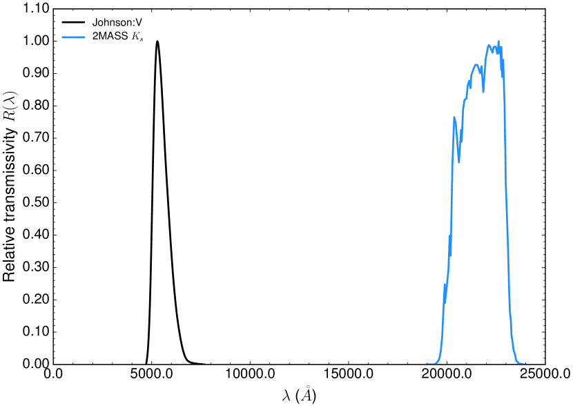
Figure 1: Relative Johnson:V (black line) and 2MASS-$K_{s}$ (blue line) transmissivity as a function of the wavelength $\lambda$.

3 Selecting MARCS model atmospheres

At this date, MARCS contains more than 52,000 atmosphere models of late-type F, G, K, and M stars. The effective temperature of MARCS model atmospheres ranges from 2500 to 8000 K, logarithmic surface gravities vary between -0.5 and 5.5, while overall logarithmic metallicities relative to the Sun $\mathrm{[Fe/H]}$ are between -5.0 and +1.0. The stellar mass can be chosen between the standard mass of 1.0 solar mass and 15 solar masses in spherical geometry. Finally, the microturbulence parameter $\xi$ can be set at 0, 1, 2, or $5\,$km.s^-1 (see Gustafsson et al. 2008 for more details).

In this work, we consider the standard composition (Grevesse et al., 2007) to simulate spectra with $T_{\mathrm{eff}}$ between 2500 K and 5000 K, $\log g$ from -1 to 5, $\mathrm{\mathrm{[Fe/H]}}$ from $-2$ to $\mathrm{[Fe/H]}=1$, and $\xi=1,2$, and $5\,$km.s^-1. For spherical models with $\log g<3$, we consider $M=1M_{\odot}$ since we show in Sect. 4.4 that the impact of the mass on the SBCR is negligible.

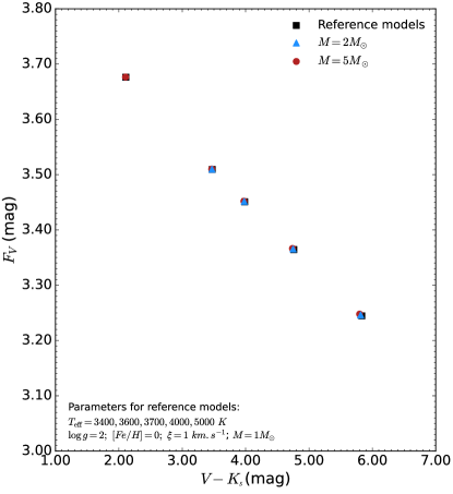
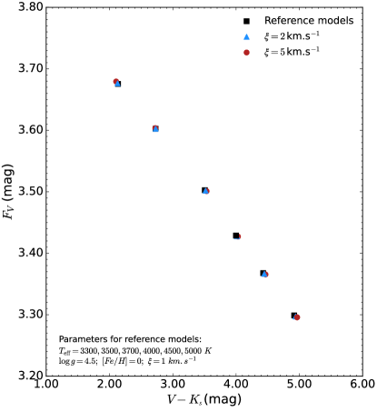
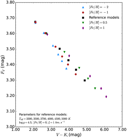
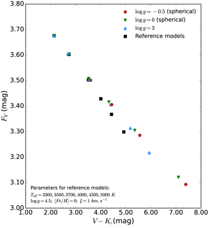
Figure 2: Influence of a change in fundamental parameters on the surface brightness of stars. Top left panel: Varying the stellar mass. Top right panel: Varying the microturbulence. Bottom left panel: Varying the metallicity. Bottom right panel: Varying the surface gravity.

4 Impact of stellar model parameters on the SBCR

4.1 Reference atmosphere models

We first define the reference models that serve as elements of comparison. We consider $T_{\mathrm{eff}}=$ 3300, 3500, 3700, 4000, 4500, 5000 K, and fix the other stellar parameters to a specific value depending on what we are studying.

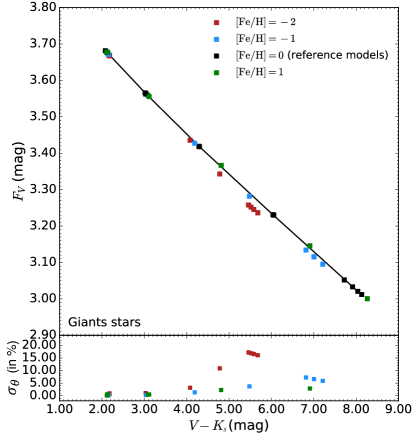
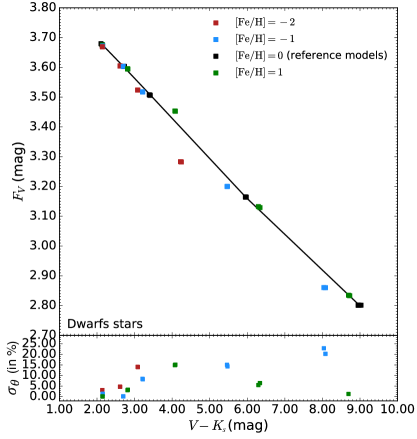
Figure 3: For giants (left) and dwarfs (right) the surface gravity $\log g$ varies with the effective temperature as shown in Table 1 (black squares), while all the parameter space of MARCS is explored regarding the microturbulence and the mass. Other colours (red, blue, and green squares) correspond to different metallicities. The bottom panels show the absolute value of the difference in the expected angular diameter between a given SBCR and the reference value (solid black line).

4.2 Microturbulence

We consider $\log g=4.5$, $\mathrm{[Fe/H]}=0$, and vary the microturbulence from $\xi=1\,$km.s^-1 to $\xi=5\,$km.s^-1. Results are shown in the top right panel of Fig. 2. We see from these plots that both the surface brightness $F_{V}$ and the $V-K_{s}$ colour are only slightly sensitive to the microturbulence. In particular, both $F_{V}$ and $V-K_{s}$ values are shifted along the SBCR, which means that neither the slope nor the zero-point of the SBCR depends on the microturbulence. We conclude that the SBCR does not depend on the microturbulence of stars.

Table 1: Corresponding $\log g$ values to effective temperatures of giant (top) and dwarf (bottom) stars.

$(V-K_{s})$	$T_{\mathrm{eff}}$	$\log g$
$[\mathrm{mag}]$	$[K]$
Giants
2.1	5000	3.0
3.0	4250	2.0
4.3	3700	1.0
6.0	3400	0.5
8.0	3200	0.0
Dwarfs
2.1	5000	4.5
2.8	4500	4.5
3.4	4000	5.0
5.9	3000	5.0
9.0	2500	5.0

4.3 Stellar metallicity

To estimate the impact of the stellar metallicity $\mathrm{[Fe/H]}$, we simulate spectra with the following metallicities $\mathrm{[Fe/H]}$: -2, 1, 0, 0.5, and 1. The change in surface brightness of stars can be seen in the bottom left panel of Fig. 2.

Increasing the metallicity leads to a decrease in the surface brightness and an increase in the colour of the star. This shift is negligibly small at $T_{\mathrm{eff}}\sim 5000\,$K and gradually increases at lower $T_{\mathrm{eff}}$. An offset of 0.025 magnitude in $F_{\mathrm{V}}$ (or 10% on the angular diameter) is expected for a variation of one dex in $\mathrm{[Fe/H]}$ at $V-K_{s}\sim 4$.

4.4 Stellar surface gravity

We studied the impact of stellar surface gravity on the surface brightness. We used models with $\log g$: -0.5, 0, 3, and 4.5. In MARCS the models with $\log g<3$ (resp. $\log g>3$) are in spherical (resp. plane-parallel) geometry. To study the consistency of mixing different geometries, we compared plane-parallel and spherical models with the same parameters. At $\log g=3$ the difference is 0.05% on the surface brightness of stars. Models in spherical geometry exist for different masses. In order to test this we considered the reference models described in Sect. 4.1 and set the mass to $M=2M_{\odot}$ and $M=5M_{\odot}$. We considered a value of $\log g=2$. The result is shown in the top left panel of Fig. 2. We conclude that the impact of the mass is negligible in our study.

The bottom right panel of Fig. 2 shows the influence of a change in surface gravity on the surface brightness deduced from atmosphere models, between $\log g=-0.5$ and $\log g=4.5$. For $V-K_{s}$ larger than about 3 (i.e. $T_{\mathrm{eff}}=4000\,$K) both $F_{V}$ and the $V-K_{s}$ colour are strongly affected by $\log g$. For a star with $V-K_{s}=4$, the difference in surface brightness ($F_{\mathrm{V}}$) for $\log g=$ -0.5, 0, and 3 is about 0.01 magnitude (or 5% on the angular diameter), while it is significantly different for $\log g=$ 4.5 (about 0.025 magnitude or 10% in angular diameter).

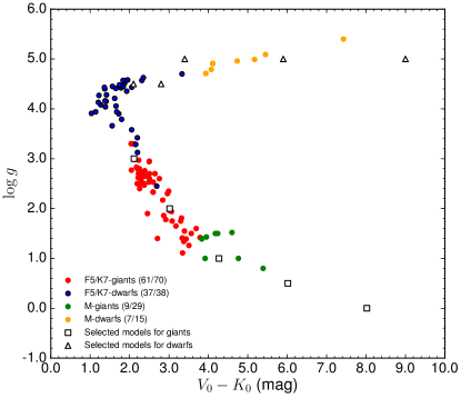
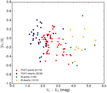
Figure 4: Fundamental parameters of stars in empirical samples of Paper I. Left panel: $\log g$ vs $V_{0}-K_{0}$ compared to coefficients from Bessell et al. (1998) (see Table 1). Right panel: $\mathrm{[Fe/H]}$ vs $V_{0}-K_{0}$. The models used for the comparison of theoretical and empirical SBCRs have solar metallicities [Fe/H]=0.

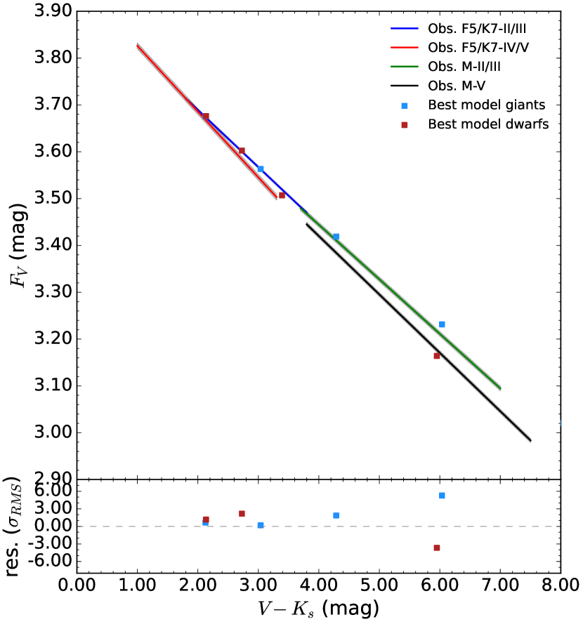
Figure 5: Comparison between 2MASS-$K_{s}$ SBCRs from Paper II and theoretical surface brightnesses calculated from stellar MARCS atmosphere models defined in Table 1, i.e. with a $\log g$ varying with the effective temperature. The metallicity is considered to be solar. The shaded grey area corresponds to the 1$\sigma$ confidence interval of the empirical SBCRs (corresponding in some cases to the thickness of the line). The lower panel shows the difference between the models and the corresponding SBCR (giants or dwarfs, respectively) in a fraction of the RMS of the empirical SBCR.

Actually giants stars, but also dwarfs, have their surface gravity that varies with $T_{\mathrm{eff}}$. By considering standard evolution models, we can consider specific sets of models, as shown in Table 1 (Bessell et al., 1998), that are also used for the comparison with observations in next section. In Fig. 3 we show the corresponding SBCRs (black line) in the case of giants (left) and dwarfs (right). We note that there are more than five references models (black squares) because we explore the entire parameter space of MARCS models in term of microturbulence and mass. In this plot we also add the values of the surface brightness for different metallicities. For the sake of clarity, we do not consider the case of $\mathrm{[Fe/H]}=-0.5$. We find that the effect of metallicity on the SBCR is larger for dwarfs than for giants. It is also larger when considering larger $V-K_{s}$ values, and this is particularly true for metal-poor stars with [Fe/H]$=-2$ dex.

Thus, the theoretical analysis shows that the SBCR is insensitive to microturbulence. It is, however, sensitive to metallicity and stellar surface gravity. The effect of metallicity was already suggested by Kervella et al. (2004c) and Boyajian et al. (2012), while the dependence of the SBCR with the class has already been observed through several works, such as Fouque & Gieren (1997); Kervella et al. (2004c); Groenewegen (2004) and Boyajian et al. (2014). However, no theoretical approach has been provided to date, except the one presented in Mould (2019). We come back to these results in the Conclusion.

5 Comparison of theoretical and empirical SBCRs

We performed a very first comparison of observations from paper I with the MARCS models. In Paper I, we implement four precise SBCRs (converted into uniform 2MASS-$K_{s}$ SBCRs in Paper II) for F5–K7 giants, F5–K7 subgiants or dwarfs, M giants, and M dwarfs stars. We cross-matched the empirical samples from Paper I with the various references in the literature (using SIMBAD queries) in order to recover the surface gravity and the metallicity.

Over 152 stars, we found 114 values of $\log g$ and 113 values of $\mathrm{[Fe/H]}$ (see Table LABEL:Tab_logg). We plot the $\log g$ and $\mathrm{[Fe/H]}$ values as a function of $V_{0}-K_{0}$ in Fig. 4.

We find that the stars used to calibrate the four SBCRs have solar metallicities on average, with a standard deviation of at most 0.5 dex in [Fe/H], which basically corresponds to the step in the MARCS grid. For $\log g$, we see that our reference models as indicated in Table 1 (i.e. open squares for giants and open triangles for dwarfs), are consistent with observations.

Finally, for a consistent comparison, we consider the set of models of Table 1 with solar metallicity. The microturbulence and the mass, as shown previously, have little impact on the surface brigthness and are set to $0$ km.s^-1 and 1 solar mass, respectively. Two models are rejected in Table LABEL:Tab_logg because they exceed the $V-K_{s}$ validity domain of the empirical relations. We end up with eight models for the comparison.
The results are shown in Fig. 5 and can be summarised as follows. The empirical 2MASS-$K_{s}$ SBCRs for F5–K7 stars (dwarfs or giants) are systematically 1–2$\sigma$ brighter than the theoretical ones. As the RMS of the empirical relations are of 0.004 and 0.002 magnitude in $F_{\mathrm{V}}$ respectively for dwarfs and giants, this difference corresponds to 0.002–0.008 magnitude in $F_{\mathrm{V}}$ or a 1–4% at most in terms of angular diameter. For M stars (dwarfs or giants), the difference between the observations and the MARCS models is larger, between 5 and 6$\sigma$. Interestingly, the empirical SBCR for giants is brighter than the theoretical one, while it is the contrary for the dwarfs. The RMS of the empirical relations are of 0.004 and 0.005 magnitude in $F_{\mathrm{V}}$ respectively for dwarfs and giants. This difference corresponds to around 10% in terms of angular diameter.

In this analysis, it is not excluded that the zero-points of the theoretical SBCRs are affected by the filters and/or the reference star used for the calculation of the synthetic magnitudes. We used Vega as a reference star, while it is known to be a pole-on fast rotator (Aufdenberg et al., 2006).

If we use instead the STIS/CALSPEC Sirius spectrum (Bohlin et al., 2020) to calculate the photometric zero-point, we find -21.12 mag instead of -21.09 mag. This offset of 0.03 magnitude on the reference star leads to an offset of 0.003 magnitude on $F_{\mathrm{V}}$, which corresponds to a 1–1.5 RMS of the empirical SBCRs. Using $\eta$ UMa as reference, considering its STIS/CALSPEC spectrum (Bohlin et al., 2020), leads to a zero-point of -21.07 mag, corresponding to a difference of $\sim$0.002 mag on $F_{\mathrm{V}}$. Such offsets only partially explain the difference observed when comparing empirical and theoretical SBCRs. Interestingly, there is one single existing filter for the 2MASS-$K_{s}$ magnitude. This is a strong advantage compared to the various Johnson $K$ filters we can find in the literature. By choosing the 2MASS-$K_{s}$ photometry in this study, we excluded any bias that could be induced by the choice of the filter.

Another possible bias can be the filter from which the synthetic $m_{V}$ magnitude is computed. The stellar flux is integrated over a wavelength range and a transmissivity that are both specific to the filter. We made a test by using the generic Johnson:V filter of Bessell et al. (1998). With this filter, the zero-point is found to be -21.12 mag. We observe a constant difference of 0.006 mag on $F_{\mathrm{V}}$ with respect to the Mann & von Braun (2015) filter. A change in the filter and/or in the reference star can lead to a better agreement between zero-points of empirical and theoretical relations, but cannot fully explain the differences obtained, in particular for M stars.

6 Discussion

6.1 Effect of the metallicity on the LMC distance

Recently, Pietrzyński et al. (2019) have established the distance to LMC with a precision of 1% using a SBCR based on 41 Galactic red clump giant stars (Gallenne et al., 2018). The metallicity of the stars ranges from -0.66 to 0.34 dex (see Gallenne et al. (2018), with an average of $-0.01\pm 0.07$ dex, while the metallicity of the LMC is of about -0.4 dex (Choudhury et al., 2016, 2021). To test the impact of metallicity on the SBCR and the distance of LMC, we compare theoretical SBCRs with metallicities of $\mathrm{[Fe/H]}=0.0$ and $\mathrm{[Fe/H]}=-0.5$ in Fig. 6. The difference in the derived angular diameter ($\theta_{\mathrm{LD}}$) using both SBCRs is less than 0.4% over the colour domain of validity of the Pietrzyński et al. (2019) relation, with an average of about 0.25% (see lower panel of Fig. 6). This basically means that a decrease in $\mathrm{[Fe/H]}$ of 0.5 dex on the SBCR leads to an increase in the LMC distance of at most 0.25% (or 0.25$\sigma$ when considering the precision of the distance of LMC established by Pietrzyński et al. 2019). In the figure we also show for comparison the empirical SBCRs of Pietrzyński et al. (2019), and of Paper I and Paper II. These SBCRs are consistent, but they are slightly shifted to brighter surface brightenesses compared to the theoretical SBCRs.

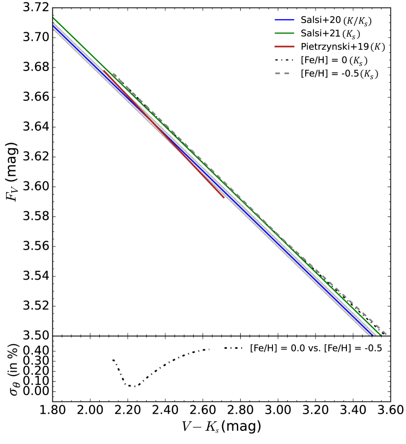
Figure 6: Comparison of theoretical SBCRs based on atmosphere models with metallicity of $\mathrm{[Fe/H]}=0.0$ and $\mathrm{[Fe/H]}=-0.5$, respectively. The empirical SBCRs from Paper I, Paper II, and Pietrzyński et al. (2019) are overplotted for comparison. The difference in the derived angular diameter $\theta_{\mathrm{LD}}$ (in %) using the two theoretical relations of different metallicity is shown in the bottom panel.

6.2 Theoretical SBCRs for Cepheids

The period-luminosity relation of Cepheids (Breuval et al., 2020) is used to calibrate the Hubble–Lemaitre constant $H_{0}$ (Riess et al., 2016, 2021). However, the different versions of the Baade–Wesselink (BW) method of distance determination, based on a SBCR (Storm et al., 2011a, b), interferometric observations (Kervella et al., 2004b), or even both (Trahin et al., 2021), are currently not used to calibrate $H_{0}$, mainly because of the projection factor (Nardetto et al., 2004, 2017) and circumstellar environment issues (Hocdé et al., 2020, 2021; Gallenne et al., 2021). In this context, the calibration of the SBCR of Cepheids is crucial in order to better understand the physics of Cepheids. Our aim here is to compare the SBCR usually used for the application of the BW (i.e. Kervella et al. 2004a), and the theoretical one. For this, we consider several atmosphere models within the Cepheid instability strip (Trahin et al., 2021), as indicated in Table 2. We consider a solar metallicity of $\mathrm{[Fe/H]}=0$. In Fig. 7 we show a comparison between the theoretical SBCR for Cepheids and the empirical SBCR of Kervella et al. (2004a). The difference is lower than 0.3$\sigma$ over the whole validity domain. This result shows an excellent agreement between theoretical and empirical SBCRs for Cepheids.

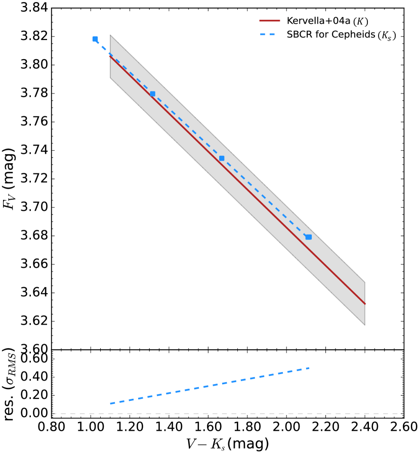
Figure 7: Comparison between the theoretical SBCR for Cepheids and the empirical relation from Kervella et al. (2004a). The lower panel shows the difference in fraction of RMS.

Table 2: Corresponding $\log g$ values to effective temperatures of Cepheid stars.

$(V-K_{s})$	$T_{\mathrm{eff}}$	$\log g$
$[\mathrm{mag}]$	$[K]$
Cepheids
1.0	6500	2.5
1.3	6000	2.0
1.6	5500	1.5
2.1	5000	1.0
2.1	5000	0.5

7 Conclusion and perspectives

In Paper I we showed that empirical SBCRs are dependant on the luminosity class of stars. By using the MARCS model atmospheres in this paper, we have theoretically analysed the influence of fundamental stellar parameters on the surface brightness of stars. We confirm the result of Paper I, and we show that SBCRs vary with the surface gravity of stars, and therefore depend on the luminosity class. Though the effect of mass and microturbulence is weak, we have shown that the metallicity also impacts the SBCR. The metallicity should therefore be taken into consideration when calibrating and using a SBCR. In this respect, we show that a difference in metallicity of 0.5 dex in the calibration of SBCRs does not impact the LMC distance by more than 0.4% (with an average difference of 0.25%).

For the first time, we have compared empirical and theoretical SBCRs. We find a very good agreement of about 1–2$\sigma$ level for F5–K7 stars, while it is of 5–6$\sigma$ for M stars. Such discrepancies, on the theoretical side, could be partly due to the choice of the reference star and/or the filter used in the models. On the observation side, it is not excluded that some stars, in particular M giants stars, are affected by dust environment, which might alter the colour estimate.

Finally, by comparing the theoretical SBCR for Cepheids with the empirical one used in the BW method of distance determination (Kervella et al., 2004a) we find an excellent agreement, better than 0.3$\sigma$.

Appendix A Additional table

Table 3: Characteristics of empirical samples from Paper I.

Star HD	Box	$V_{0}-K_{0}$	$\log g$	$\mathrm{[Fe/H]}$	Source
		[mag]
HD 10142	1	2.37	2.47	-0.15	Alves et al. (2015)
HD 102328	1	2.76	2.60	0.26	Lomaeva et al. (2019)
HD 113226	1	2.05	2.77	0.05	Park et al. (2018)
HD 11977	1	2.19	2.50	-	Bonfanti et al. (2016)
HD 120477	1	3.69	1.60	-0.57	Hekker & Meléndez (2007)
HD 127665	1	2.96	2.30	-0.19	Hekker & Meléndez (2007)
HD 133124	1	3.51	1.26	-0.11	Lomaeva et al. (2019)
HD 13468	1	2.25	2.80	-0.12	Hekker & Meléndez (2007)
HD 135722	1	2.27	2.63	-0.34	Lomaeva et al. (2019)
HD 136726	1	3.06	1.94	0.00	Maldonado & Villaver (2016)
HD 153210	1	2.50	2.70	0.07	Hekker & Meléndez (2007)
HD 157681	1	3.34	1.11	-0.24	Lomaeva et al. (2019)
HD 163770	1	2.71	1.40	0.25	Fernandez-Villacanas et al. (1990)
HD 164058	1	3.39	1.55	-0.23	Lambert & Ries (1981)
HD 16815	1	2.41	2.65	-0.34	Alves et al. (2015)
HD 170693	1	2.87	1.86	-0.49	Lomaeva et al. (2019)
HD 176678	1	2.50	2.95	0.02	Hekker & Meléndez (2007)
HD 17709	1	3.79	1.42	-0.36	McWilliam (1990)
HD 17824	1	2.10	3.30	0.07	Hekker & Meléndez (2007)
HD 184293	1	2.92	1.78	-0.37	Lomaeva et al. (2019)
HD 185958	1	2.21	2.79	-0.03	McWilliam (1990)
HD 18784	1	2.38	2.76	0.09	Zhao et al. (2001)
HD 192781	1	3.44	1.39	-0.23	Lomaeva et al. (2019)
HD 19787	1	2.28	2.69	0.09	Arentsen et al. (2019)
HD 200205	1	3.34	1.41	-0.38	Lomaeva et al. (2019)
HD 204381	1	2.04	3.30	-0.02	Hekker & Meléndez (2007)
HD 211388	1	3.08	1.75	-0.12	McWilliam (1990)
HD 214868	1	3.01	1.96	-0.15	Lomaeva et al. (2019)
HD 215665	1	2.26	2.40	-0.06	Thygesen et al. (2012)
HD 216131	1	2.13	2.99	0.02	Deka-Szymankiewicz et al. (2018)
HD 216131	1	2.13	2.99	0.02	Deka-Szymankiewicz et al. (2018)
HD 219449	1	2.49	2.53	0.00	Lomaeva et al. (2019)
HD 220572	1	2.36	2.73	0.08	Liu et al. (2007)
HD 23526	1	2.26	2.50	-0.15	Liu et al. (2014)
HD 23940	1	2.29	2.52	-0.34	Alves et al. (2015)
HD 30504	1	3.30	1.75	-0.36	McWilliam (1990)
HD 30814	1	2.23	2.97	-0.07	McWilliam (1990)
HD 3546	1	2.17	2.83	-0.50	da Silva et al. (2015)
HD 360	1	2.32	2.73	-0.07	Liu et al. (2007)
HD 36848	1	2.64	2.70	0.28	da Silva et al. (2006)
HD 36874	1	2.51	2.54	0.00	Jones et al. (2011)
HD 3750	1	2.50	2.60	0.03	Liu et al. (2007)
HD 39523	1	2.45	1.90	0.15	Proust (1984)
HD 39640	1	2.23	2.70	-0.11	Alves et al. (2015)
HD 4211	1	2.60	2.53	-0.01	Liu et al. (2007)
HD 46116	1	2.26	2.63	-0.32	Alves et al. (2015)
HD 5722	1	2.22	2.70	-0.18	Hekker & Meléndez (2007)
HD 60060	1	2.31	2.72	-0.08	Alves et al. (2015)
HD 60341	1	2.50	2.94	0.04	da Silva et al. (2015)
HD 69267	1	3.37	1.34	-0.30	Sousa et al. (2018)
HD 76294	1	2.22	2.62	-0.07	Lomaeva et al. (2019)
HD 83618	1	2.99	2.35	-0.07	Hekker & Meléndez (2007)
HD 85503	1	2.65	-	0.21	Casamiquela et al. (2019)
HD 8651	1	2.39	2.66	-0.20	Alves et al. (2015)
HD 87837	1	3.32	1.81	-0.02	McWilliam (1990)
HD 9362	1	2.30	2.60	-0.29	Alves et al. (2015)
HD 9408	1	2.35	2.51	-0.26	da Silva et al. (2015)
HD 96833	1	2.60	2.33	-0.07	Lomaeva et al. (2019)
HD 96833	1	2.60	2.33	-0.07	Lomaeva et al. (2019)
HD 98262	1	3.18	1.65	-0.14	Lomaeva et al. (2019)
HD 9927	1	2.84	2.17	0.11	Maldonado & Villaver (2016)
HD 99998	1	3.57	1.50	-0.36	Arentsen et al. (2019)
HD 102870	2	1.27	4.08	0.14	Luck (2017)
HD 10476	2	1.95	4.58	0.02	Luck (2017)
HD 10697	2	1.67	3.94	0.12	Luck (2017)
HD 10700	2	1.84	4.45	-0.51	Hojjatpanah et al. (2019)
HD 114710	2	1.37	4.40	0.06	Luck (2017)
HD 117176	2	1.73	3.90	-0.09	Luck (2017)
HD 140283	2	1.56	3.66	-2.43	Arentsen et al. (2019)
HD 140538	2	1.57	4.45	0.01	Luck (2017)
HD 142860	2	1.21	4.13	-0.12	Luck (2017)
HD 158633	2	1.90	4.57	-0.41	Luck (2017)
HD 16160	2	2.35	4.63	-	Hojjatpanah et al. (2019)
HD 168723	2	2.20	3.13	-0.16	Hojjatpanah et al. (2019)
HD 173667	2	1.14	3.94	0.09	Luck (2017)
HD 173701	2	1.84	4.45	0.36	Grieves et al. (2018)
HD 175726	2	1.36	4.43	-0.04	Luck (2017)
HD 182572	2	1.62	4.21	0.41	Hojjatpanah et al. (2019)
HD 185144	2	1.83	4.57	-0.08	Luck (2017)
HD 187637	2	1.22	4.27	-0.12	Furlan et al. (2018)
HD 188512	2	2.05	3.58	-0.19	Luck (2017)
HD 188887	2	2.69	2.45	0.11	Liu et al. (2007)
HD 190360	2	1.65	4.41	0.27	Hojjatpanah et al. (2019)
HD 19373	2	1.41	4.15	0.11	Luck (2017)
HD 195564	2	1.66	4.06	0.08	Hojjatpanah et al. (2019)
HD 198149	2	2.20	3.42	-0.12	Luck (2017)
HD 19994	2	1.39	4.04	0.19	Luck (2017)
HD 21019	2	1.80	3.79	-0.43	Luck (2017)
HD 219134	2	2.31	4.57	0.06	Park et al. (2018)
HD 22484	2	1.38	4.16	-0.01	Hojjatpanah et al. (2019)
HD 30652	2	1.03	3.91	-	Hojjatpanah et al. (2019)
HD 34411	2	1.41	4.28	0.09	Luck (2017)
HD 3651	2	1.88	4.52	0.24	Luck (2017)
HD 38858	2	1.74	4.48	-0.12	Luck (2017)
HD 4628	2	2.06	4.43	-0.34	Hojjatpanah et al. (2019)
HD 69830	2	1.78	4.42	-0.03	Hojjatpanah et al. (2019)
HD 75732	2	1.93	4.35	0.34	Hojjatpanah et al. (2019)
HD 88230	2	3.33	4.70	0.21	Luck (2017)
HD 90043	2	2.15	3.29	-0.01	Hojjatpanah et al. (2019)
HD 1013	3	4.18	1.50	-	Massarotti et al. (2008)
HD 102212	3	3.95	1.43	-0.54	Arentsen et al. (2019)
HD 120933	3	4.60	1.52	0.50	McWilliam (1990)
HD 121130	3	4.76	1.00	-0.24	Smith & Lambert (1986)
HD 183439	3	3.83	1.40	-0.38	Smith & Lambert (1986)
HD 18884	3	4.24	1.50	-0.60	Lebzelter et al. (2012)
HD 19058	3	5.39	0.80	-0.15	Smith & Lambert (1986)
HD 218329	3	3.83	1.39	-0.20	Boeche & Grebel (2016)
HD 25025	3	3.92	1.00	-	Massarotti et al. (2008)
GJ406	4	7.43	5.40	-	Rajpurohit et al. (2018)
GJ447	4	5.45	5.09	-0.04	Schweitzer et al. (2019)
GJ581	4	4.73	4.96	0.21	Park et al. (2018)
GJ674	4	4.55	-	-0.26	Hojjatpanah et al. (2019)
GJ687	4	4.65	-	0.03	Gaidos et al. (2014)
GJ876	4	5.17	4.99	-	Schweitzer et al. (2019)
HD 119850	4	4.07	4.79	-	Arentsen et al. (2019)
HD 1326	4	4.11	4.91	-0.25	Schweitzer et al. (2019)
HD 199305	4	3.94	4.71	0.04	Schweitzer et al. (2019)
HD 204961	4	4.19	-	-0.19	Hojjatpanah et al. (2019)
HD 225213	4	4.09	-	-0.51	Hojjatpanah et al. (2019)
HD 36395	4	3.80	-	0.19	Hojjatpanah et al. (2019)
HIP51397	4	4.32	-	-0.22	Hojjatpanah et al. (2019)

Table 3: Continued.

References

- Alves et al. (2015) Alves, S., Benamati, L., Santos, N. C., et al. 2015, MNRAS, 448, 2749
- Arentsen et al. (2019) Arentsen, A., Prugniel, P., Gonneau, A., et al. 2019, A&A, 627, A138
- Aufdenberg et al. (2006) Aufdenberg, J. P., Mérand, A., Coudé du Foresto, V., et al. 2006, ApJ, 645, 664
- Barnes & Evans (1976) Barnes, T. G. & Evans, D. S. 1976, MNRAS, 174, 489
- Bessell et al. (1998) Bessell, M. S., Castelli, F., & Plez, B. 1998, A&A, 333, 231
- Boeche & Grebel (2016) Boeche, C. & Grebel, E. K. 2016, A&A, 587, A2
- Bohlin et al. (2020) Bohlin, R., Deustua, S., & De Rosa, G. 2020, in American Astronomical Society Meeting Abstracts, Vol. 235, American Astronomical Society Meeting Abstracts #235, 372.01
- Bohlin et al. (2014) Bohlin, R. C., Gordon, K. D., & Tremblay, P. E. 2014, PASP, 126, 711
- Bonfanti et al. (2016) Bonfanti, A., Ortolani, S., & Nascimbeni, V. 2016, A&A, 585, A5
- Boyajian et al. (2014) Boyajian, T. S., van Belle, G. T., & von Braun, K. 2014, AJ, 147, 47
- Boyajian et al. (2012) Boyajian, T. S., von Braun, K., van Belle, G., et al. 2012, ApJ, 757, 112
- Breuval et al. (2020) Breuval, L., Kervella, P., Anderson, R. I., et al. 2020, A&A, 643, A115
- Casamiquela et al. (2019) Casamiquela, L., Blanco-Cuaresma, S., Carrera, R., et al. 2019, MNRAS, 490, 1821
- Catala & PLATO Team (2006) Catala, C. & PLATO Team. 2006, ESA Special Publication, 1306, 497
- Challouf et al. (2014) Challouf, M., Nardetto, N., Mourard, D., et al. 2014, A&A, 570, A104
- Choudhury et al. (2021) Choudhury, S., de Grijs, R., Bekki, K., et al. 2021, MNRAS, 507, 4752
- Choudhury et al. (2016) Choudhury, S., Subramaniam, A., & Cole, A. A. 2016, MNRAS, 455, 1855
- Cohen et al. (2003) Cohen, M., Wheaton, W. A., & Megeath, S. T. 2003, AJ, 126, 1090
- Cutri et al. (2003) Cutri, R. M., Skrutskie, M. F., van Dyk, S., et al. 2003, VizieR Online Data Catalog, II/246
- da Silva et al. (2006) da Silva, L., Girardi, L., Pasquini, L., et al. 2006, A&A, 458, 609
- da Silva et al. (2015) da Silva, R., Milone, A. d. C., & Rocha-Pinto, H. J. 2015, A&A, 580, A24
- Deka-Szymankiewicz et al. (2018) Deka-Szymankiewicz, B., Niedzielski, A., Adamczyk, M., et al. 2018, A&A, 615, A31
- Duvert (2016) Duvert, G. 2016, VizieR Online Data Catalog, II/345
- Fernandez-Villacanas et al. (1990) Fernandez-Villacanas, J. L., Rego, M., & Cornide, M. 1990, AJ, 99, 1961
- Fouque & Gieren (1997) Fouque, P. & Gieren, W. P. 1997, A&A, 320, 799
- Furlan et al. (2018) Furlan, E., Ciardi, D. R., Cochran, W. D., et al. 2018, ApJ, 861, 149
- Gaidos et al. (2014) Gaidos, E., Mann, A. W., Lépine, S., et al. 2014, MNRAS, 443, 2561
- Gallenne et al. (2021) Gallenne, A., Mérand, A., Kervella, P., et al. 2021, A&A, 651, A113
- Gallenne et al. (2018) Gallenne, A., Pietrzyński, G., Graczyk, D., et al. 2018, A&A, 616, A68
- Graczyk et al. (2020) Graczyk, D., Pietrzyński, G., Thompson, I. B., et al. 2020, ApJ, 904, 13
- Grevesse et al. (2007) Grevesse, N., Asplund, M., & Sauval, A. J. 2007, Space Sci. Rev., 130, 105
- Grieves et al. (2018) Grieves, N., Ge, J., Thomas, N., et al. 2018, MNRAS, 481, 3244
- Groenewegen (2004) Groenewegen, M. A. T. 2004, MNRAS, 353, 903
- Gustafsson et al. (2008) Gustafsson, B., Edvardsson, B., Eriksson, K., et al. 2008, A&A, 486, 951
- Hekker & Meléndez (2007) Hekker, S. & Meléndez, J. 2007, A&A, 475, 1003
- Hocdé et al. (2020) Hocdé, V., Nardetto, N., Lagadec, E., et al. 2020, A&A, 633, A47
- Hocdé et al. (2021) Hocdé, V., Nardetto, N., Matter, A., et al. 2021, A&A, 651, A92
- Hojjatpanah et al. (2019) Hojjatpanah, S., Figueira, P., Santos, N. C., et al. 2019, A&A, 629, A80
- Jones et al. (2011) Jones, M. I., Jenkins, J. S., Rojo, P., & Melo, C. H. F. 2011, A&A, 536, A71
- Kervella et al. (2004a) Kervella, P., Bersier, D., Mourard, D., et al. 2004a, A&A, 428, 587
- Kervella et al. (2004b) Kervella, P., Nardetto, N., Bersier, D., Mourard, D., & Coudé du Foresto, V. 2004b, A&A, 416, 941
- Kervella et al. (2004c) Kervella, P., Thévenin, F., Di Folco, E., & Ségransan, D. 2004c, A&A, 426, 297
- Lambert & Ries (1981) Lambert, D. L. & Ries, L. M. 1981, ApJ, 248, 228
- Lebzelter et al. (2012) Lebzelter, T., Heiter, U., Abia, C., et al. 2012, A&A, 547, A108
- Liu et al. (2014) Liu, Y. J., Tan, K. F., Wang, L., et al. 2014, ApJ, 785, 94
- Liu et al. (2007) Liu, Y. J., Zhao, G., Shi, J. R., Pietrzyński, G., & Gieren, W. 2007, MNRAS, 382, 553
- Lomaeva et al. (2019) Lomaeva, M., Jönsson, H., Ryde, N., Schultheis, M., & Thorsbro, B. 2019, A&A, 625, A141
- Luck (2017) Luck, R. E. 2017, AJ, 153, 21
- Maldonado & Villaver (2016) Maldonado, J. & Villaver, E. 2016, A&A, 588, A98
- Mamajek et al. (2015) Mamajek, E. E., Torres, G., Prsa, A., et al. 2015, arXiv e-prints, arXiv:1510.06262
- Mann & von Braun (2015) Mann, A. W. & von Braun, K. 2015, PASP, 127, 102
- Massarotti et al. (2008) Massarotti, A., Latham, D. W., Stefanik, R. P., & Fogel, J. 2008, AJ, 135, 209
- McWilliam (1990) McWilliam, A. 1990, ApJS, 74, 1075
- Meftah et al. (2018) Meftah, M., Corbard, T., Hauchecorne, A., et al. 2018, A&A, 616, A64
- Mould (2019) Mould, J. 2019, PASP, 131, 094201
- Nardetto (2018) Nardetto, N. 2018, Habilitation Thesis
- Nardetto et al. (2004) Nardetto, N., Fokin, A., Mourard, D., et al. 2004, A&A, 428, 131
- Nardetto et al. (2017) Nardetto, N., Poretti, E., Rainer, M., et al. 2017, A&A, 597, A73
- Park et al. (2018) Park, S., Lee, J.-E., Kang, W., et al. 2018, ApJS, 238, 29
- Pietrzyński et al. (2019) Pietrzyński, G., Graczyk, D., Gallenne, A., et al. 2019, Nature, 567, 200
- Pitjeva & Standish (2009) Pitjeva, E. V. & Standish, E. M. 2009, Celestial Mechanics and Dynamical Astronomy, 103, 365
- Plez (2008) Plez, B. 2008, Physica Scripta Volume T, 133, 014003
- Price-Whelan et al. (2018) Price-Whelan, A. M., Sipőcz, B. M., Günther, H. M., et al. 2018, AJ, 156, 123
- Proust (1984) Proust, D. 1984, PhD thesis, -
- Rajpurohit et al. (2018) Rajpurohit, A. S., Allard, F., Rajpurohit, S., et al. 2018, A&A, 620, A180
- Riess et al. (2016) Riess, A. G., Macri, L. M., Hoffmann, S. L., et al. 2016, ApJ, 826, 56
- Riess et al. (2021) Riess, A. G., Yuan, W., Macri, L. M., et al. 2021, arXiv e-prints, arXiv:2112.04510
- Rodrigo & Solano (2020) Rodrigo, C. & Solano, E. 2020, in Contributions to the XIV.0 Scientific Meeting (virtual) of the Spanish Astronomical Society, 182
- Rodrigo et al. (2012) Rodrigo, C., Solano, E., & Bayo, A. 2012, SVO Filter Profile Service Version 1.0, IVOA Working Draft 15 October 2012
- Salsi et al. (2020) Salsi, A., Nardetto, N., Mourard, D., et al. 2020, A&A, 640, A2
- Salsi et al. (2021) Salsi, A., Nardetto, N., Mourard, D., et al. 2021, A&A, 652, A26
- Schweitzer et al. (2019) Schweitzer, A., Passegger, V. M., Cifuentes, C., et al. 2019, A&A, 625, A68
- Smith & Lambert (1986) Smith, V. V. & Lambert, D. L. 1986, ApJ, 311, 843
- Sousa et al. (2018) Sousa, S. G., Adibekyan, V., Delgado-Mena, E., et al. 2018, A&A, 620, A58
- Storm et al. (2011a) Storm, J., Gieren, W., Fouqué, P., et al. 2011a, A&A, 534, A94
- Storm et al. (2011b) Storm, J., Gieren, W., Fouqué, P., et al. 2011b, A&A, 534, A95
- Thygesen et al. (2012) Thygesen, A. O., Frandsen, S., Bruntt, H., et al. 2012, A&A, 543, A160
- Trahin et al. (2021) Trahin, B., Breuval, L., Kervella, P., et al. 2021, A&A, 656, A102
- van Belle (1999) van Belle, G. T. 1999, PASP, 111, 1515
- Wesselink (1969) Wesselink, A. J. 1969, MNRAS, 144, 297
- Willmer (2018) Willmer, C. N. A. 2018, ApJS, 236, 47
- Zhao et al. (2001) Zhao, G., Qiu, H. M., & Mao, S. 2001, ApJ, 551, L85
Acknowledgements.
BP acknowledges support from the CNES (Centre National d’Etudes Spatiales) in the framework of the PLATO mission. This work is based upon observations obtained with the Georgia State University Center for High Angular Resolution Astronomy Array at Mount Wilson Observatory. The CHARA Array is funded by the National Science Foundation through NSF grants AST-0606958 and AST-0908253 and by Georgia State University through the College of Arts and Sciences, as well as the W. M. Keck Foundation. This work made use of the JMMC Measured stellar Diameters Catalog (Duvert 2016). This research made use of the SIMBAD and VIZIER555Available at http://cdsweb.u-strasbg.fr/ databases at CDS, Strasbourg (France) and the electronic bibliography maintained by the NASA/ADS system. This work has made use of data from the European Space Agency (ESA) mission Gaia (https://www.cosmos.esa.int/gaia). This research also made use of Astropy, a community-developed core Python package for Astronomy (Price-Whelan et al. 2018). This research has made use of the SVO Filter Profile Service666http://svo2.cab.inta-csic.es/theory/fps/ supported from the Spanish MINECO through grant AYA2017-84089.Appendix A Additional table