In this section, we illustrate our main result with a simple experiment. We follow the same problem setting as that of WT2011 in Section 5.1. That is, we aim to sample from a non-log-concave posterior distribution $p(\theta|x)\propto p(\theta)\prod_{i=1}^{n}p(x_{i}|\theta)$ where $\{x_{i}\}_{i=1}^{n}$ is sampled from $p(x|\theta)$, a distribution parameterized by $\theta=(\theta_{1},\theta_{2})$. The prior $p(\theta)$ and the distribution of $x$ parametrized by $\theta$ are respectively defined as $\theta_{1}\sim N(0,10)$, $\theta_{2}\sim N(0,1)$ and $x\sim 1/2N(\theta_{1},2)+1/2N(\theta_{1}+\theta_{2},2)$. Here, we set $n=10000$, $\theta_{1}=0$ and $\theta_{2}=1$. Using the obtained 10000 samples, we simulated 1000 points of SVRG-LD with the inner loop length $m=n/B$ and different batch sizes $B$, namely, 100, 1000 and 10000 so that $B\geq m$ as required in Theorem LABEL:mth1. Evolution of KL-divergence between the true posterior, estimated by the Metropolis-adjusted Langevin algorithm, and that simulated by SVRG-LD is plotted in Figure figexp11. KL-divergence was approximated following P2008.

figexp1

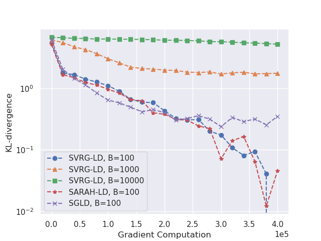
Figure 1: KL-divergence between the true and the simulated posterior. 1000 points were simulated for each algorithm with step size $\eta=0.00001$. The inner loop length $m$ for SVRG-LD was defined as $n/B$, and initial points were randomly drawn from the standard normal distribution. 1 gradient computation refers to one computation of $\nabla f_{i}$.

As we can observe, Figure figexp11 correctly reproduces the theoretical bound of Theorem LABEL:mth1, with an exponential convergence in the beginning and a persistent bias due to the use of a discrete scheme and mini-batches. The fastest convergence in terms of gradient complexity under the condition $B\geq m$ is achieved by SVRG-LD with $B=\sqrt{n}$, which confirms our main theorem. Furthermore, with this best batch size, we also simulated 1000 points of SGLD and SARAH-LD as shown in Figure figexp11 as well. While SGLD and SVRG-LD have similar convergence speed in the beginning, the latter eventually achieves a higher precision thanks to the variance reduction method adopted in this scheme. SARAH-LD exhibits a similar performance as SVRG-LD, which agrees with Theorem LABEL:mth2.