A unified analysis framework for iterative parallel-in-time algorithms

Abstract

Parallel-in-time integration has been the focus of intensive research efforts over the past two decades due to the advent of massively parallel computer architectures and the scaling limits of purely spatial parallelization. Various iterative parallel-in-time (PinT) algorithms have been proposed, like Parareal, PFASST, MGRIT, and Space-Time Multi-Grid (STMG). These methods have been described using different notations, and the convergence estimates that are available are difficult to compare. We describe Parareal, PFASST, MGRIT and STMG for the Dahlquist model problem using a common notation and give precise convergence estimates using generating functions. This allows us, for the first time, to directly compare their convergence. We prove that all four methods eventually converge super-linearly, and also compare them numerically. The generating function framework provides further opportunities to explore and analyze existing and new methods.

65R20, 45L05, 65L20

1 Introduction

The efficient numerical solution of time-dependent ordinary and partial differential equations (ODEs/PDEs) has always been an important research subject in computational science and engineering. Nowadays, with high-performance computing platforms providing more and more processors whose individual processing speeds are no longer increasing, the capacity of algorithms to run concurrently becomes important. As classical parallelization algorithms start to reach their intrinsic efficiency limits, substantial research efforts have been invested to find new parallelization approaches that can translate the computing power of modern many-core high-performance computing architectures into faster simulations.

For time-dependent problems, the idea to parallelize across the time direction has gained renewed attention in the last two decades. Various algorithms have been developed, for overviews see the papers by Gander [18] or Ong and Schroder [42]. Four iterative algorithms have received significant attention, namely Parareal [37] (474 citat. since 2001), the Parallel Full Approximation Scheme in Space and Time (PFASST) [11] (254 citat. since 2012), Multi-Grid Reduction In Time, (MGRIT) [16, 14] (287 citat. since 2014) and a specific form of Space-Time Multi-Grid (STMG) [26] (140 citat. since 2016). Other algorithms have been proposed, e.g. the Parallel (or Parareal) Implicit Time integration Algorithm PITA [15] (275 citat. since 2003) which is very similar to Parareal, the diagonalization technique [39] (63 citat. since 2008), Revisionist Integral Deferred Corrections (RIDC) [6] (114 citat. since 2010), ParaExp [20] (103 citat. since 2013) or parallel Rational approximation of EXponential Integrators (REXI) [47] (28 citat. since 2018).

Parareal, PFASST, MGRIT and STMG have all been benchmarked for large-scale problems using large numbers of cores of high-performance computing systems [34, 36, 38, 49]. They cast the solution process in time as a large linear or nonlinear system which is solved by iterating on all time steps simultaneously. Since parallel performance is strongly linked to the rate of convergence, understanding convergence mechanisms and obtaining reliable error bounds for these iterative PinT methods is crucial. Individual analyses exist for Parareal [2, 21, 27, 44, 50], MGRIT [8, 33, 48], PFASST [3, 4], and STMG [26]. There are also a few combined analyses showing equivalences between Parareal and MGRIT [14, 22] or connections between MGRIT and PFASST [40]. However, no systematic comparison of convergence behaviour, let alone efficiencies, between these methods exists.

There are at least three obstacles to comparing these four methods: first, there is no common formalism or notation to describe them; second, the existing analyses use very different techniques to obtain convergence bounds; third, the algorithms can be applied to many different problems in different ways with many tunable parameters, all of which affect performance [29]. Our main contribution is to address, at least for the Dahlquist test problem, the first two problems by proposing a common formalism to rigorously describe Parareal, PFASST, MGRIT and the Time Multi-Grid (TMG) component of STMG using the same notation. Then, we obtain comparable error bounds for all four methods by using the Generating Function Method (GFM) [35]. GFM has been used to analyze Parareal [21] and was used to relate Parareal and MGRIT [22]. However, our use of GFM to derive common convergence bounds across multiple algorithms is novel, as is the presented unified framework. When coupled with a predictive model for computational cost, this GFM framework could eventually be extended to a model to compare parallel performance of different algorithms, but this is left for future work.

Our manuscript is organized as follows: In Section 2, we introduce the GFM framework. In particular, in Section 2.1, we give three definitions (time block, block variable and block operator) used to build the GFM framework and provide some examples using classical time integration methods. Section 2.2 contains the central definition of a block iteration and again examples. In Section 2.3, we state the main theoretical results and error bounds, and the next sections contain how existing algorithms from the PinT literature can be expressed in the GFM framework: Parareal in Section 3, TMG in Section 4, and PFASST in Section 5. Finally, we compare in Section 6 all methods using the GFM framework. Conclusions and an outlook are given in Section 7.

2 The Generating Function Method

We consider the Dahlquist equation

(1) $$\frac{du}{dt}=\lambda u,\quad\lambda\in\mathbb{C},\quad t\in(0,T],\quad u(0)=u_{0}\in\mathbb{C}.$$

The complex parameter $\lambda$ allows us to emulate problems of parabolic ($\lambda<0$), hyperbolic ($\lambda$ imaginary) and mixed type.

2.1 Blocks, block variables, and block operators

We decompose the time interval $[0,T]$ into $N$ time sub-intervals $[t_{n},t_{n+1}]$ of uniform size $\Delta t$ with $n\in\{0,...,N-1\}$.

Definition 2.1 (time block).

A time block (or simply block) denotes the discretization of a time sub-interval $[t_{n},t_{n+1}]$ using $M>0$ grid points,

(2) $$\tau_{n,m}=t_{n}+\Delta t\tau_{m},\quad m\in\{1,...,M\},$$

where the $\tau_{m}\in[0,1]$ denote normalized grid points in time used for all blocks.

We choose the name “block” in order to have a generic name for the internal steps inside each time sub-interval. A block could be several time steps of a classical time-stepping scheme (e.g. Runge-Kutta, cf. Section 2.1.1), the quadrature nodes of a collocation method (cf. Section 2.1.2) or a combination of both. But in every case, a block represents the time domain that is associated to one computational process of the time parallelization. A block can also collapse by setting $M:=1$ and $\tau_{1}:=1$, so that we retrieve a standard uniform time-discretization with time step $\Delta t$. The additional structure provided by blocks will be useful when describing and analyzing two-level methods which use different numbers of grid points per block for each level, cf. Section 4.2.

Definition 2.2 (block variable).

A block variable is a vector

(3) $$\bm{u}_{n}=[u_{n,1},u_{n,2},\ldots,u_{n,M}]^{T},$$

where $u_{n,m}$ is an approximation of $u(\tau_{n,m})$ on the time block for the time sub-interval $[t_{n},t_{n+1}]$. For $M=1$, $\bm{u}_{n}$ reduces to a scalar approximation of $u(\tau_{n,M})\equiv u(t_{n+1})$.

Some iterative PinT methods like Parareal (see Section 3) use values defined at the interfaces between sub-intervals $[t_{n},t_{n+1}]$. Other algorithms, like PFASST (see Section 5), update solution values in the interior of blocks. In the first case, the block variable is the right interface value with $M=1$ and thus $\tau_{1}=1$. In the second case, it consists of volume values in the time block $[t_{n},t_{n+1}]$ with $M>1$. In both cases, PinT algorithms can be defined as iterative processes updating the block variables.

Remark 2.3.

While the adjective “time” is natural for evolution problems, PinT algorithms can also be applied to recurrence relations in different contexts like deep learning [30] or when computing Gauss quadrature formulas  [24]. Therefore, we will not systematically mention “time” when talking about blocks and block variables.

Definition 2.4 (block operators).

We denote as block operators the two linear functions $\bm{\phi}:\mathbb{C}^{M}\rightarrow\mathbb{C}^{M}$ and $\bm{\chi}:\mathbb{C}^{M}\rightarrow\mathbb{C}^{M}$ for which the block variables of a numerical solution of (1) satisfy

(4) $$\bm{\phi}(\bm{u}_{1})=\bm{\chi}(u_{0}\bm{\mbox{1I}}),\quad\bm{\phi}(\bm{u}_{n+1})=\bm{\chi}(\bm{u}_{n}),\quad n=1,2,\ldots,N-1,$$

with $\bm{\mbox{1I}}:=[1,\dots,1]^{T}$. The time integration operator $\bm{\phi}$ is bijective and $\bm{\chi}$ is a transmission operator. The time propagator updating $\bm{u}_{n}$ to $\bm{u}_{n+1}$ is given by

(5) $$\bm{\psi}:=\bm{\phi}^{-1}\bm{\chi}.$$

2.1.1 Example with Runge-Kutta methods

Consider numerical integration of (1) with a Runge-Kutta method with stability function

(6) $$R(z)\approx e^{z}.$$

Using $\ell$ equidistant time steps per block, there are two natural ways to write the method using block operators:

1. The volume formulation: set $M:=\ell$ with $\tau_{m}:=m/M$, $m=1,\ldots,M$. Setting $r:=R(\lambda\Delta t/\ell)^{-1}$, the block operators are the $M\times M$ sparse matrices

   (7) $$\bm{\phi}:=\begin{pmatrix}r&\\ -1&r&\\ &\ddots&\ddots\end{pmatrix},\quad\bm{\chi}:=\begin{pmatrix}0&\dots&0&1\\ \vdots&&\vdots&0\\ \vdots&&\vdots&\vdots\end{pmatrix}.$$

2. The interface formulation: set $M:=1$ so that

   (8) $$\bm{\phi}:=R(\lambda\Delta t/\ell)^{-\ell},\quad\bm{\chi}:=1.$$

2.1.2 Example with collocation methods

Collocation methods are special implicit Runge-Kutta methods [52, Chap. IV, Sec. 4] and instrumental when defining PFASST in Section 5. We show their representation with block operators. Starting from the Picard formulation for (1) in one time sub-interval $[t_{n},t_{n+1}]$,

(9) $$u(t)=u(t_{n})+\int_{t_{n}}^{t}\lambda u(\tau)d\tau,$$

we choose a quadrature rule to approximate the integral. We consider only Lobatto or Radau-II type quadrature nodes where the last quadrature node coincides with the right sub-interval boundary. This gives us quadrature nodes for each sub-interval that form the block discretization points $\tau_{n,m}$ of Definition 2.1, with $\tau_{M}=1$. We approximate the solution $u(\tau_{n,m})$ at each node by

(10) $$u_{n,m}=u_{n,0}+\lambda\Delta t\sum_{j=1}^{M}q_{m,j}u_{n,j}\quad\text{with}\quad q_{m,j}:=\int_{0}^{\tau_{m}}l_{j}(s)ds,$$

where $l_{j}$ are the Lagrange polynomials associated with the nodes $\tau_{m}$. Combining all the nodal values, we form the block variable $\bm{u}_{n}$, which satisfies the linear system

(11) $$(\mathbf{I}-\mathbf{Q})\bm{u}_{n}=\begin{pmatrix}u_{n,0}\\ \vdots\\ u_{n,0}\end{pmatrix}=\begin{bmatrix}0&\dots&0&1\\ \vdots&&\vdots&\vdots\\ 0&\dots&0&1\end{bmatrix}\bm{u}_{n-1}=:\mathbf{H}\bm{u}_{n-1},$$

with the quadrature matrix $\mathbf{Q}:=\lambda\Delta t(q_{m,j})$, $\mathbf{I}$ the identity matrix, and $\mathbf{H}$ sometimes called the transfer matrix that copies the last value of the previous time block to obtain the initial value $u_{n,0}$ of the current block. The integration and transfer block operators from Definition 2.4 then become $\bm{\phi}:=(\mathbf{I}-\mathbf{Q})$, $\bm{\chi}:=\mathbf{H}$.

2.2 Block iteration

Having defined the block operators for our problem, we write the numerical approximation (4) of (1) as the all-at-once global problem

(12) $$\mathbf{A}\bm{u}:=\begin{pmatrix}\bm{\phi}&&&\\ -\bm{\chi}&\bm{\phi}&&\\ &\ddots&\ddots&\\ &&-\bm{\chi}&\bm{\phi}\end{pmatrix}\begin{bmatrix}\bm{u}_{1}\\ \bm{u}_{2}\\ \vdots\\ \bm{u}_{N}\end{bmatrix}=\begin{bmatrix}\bm{\chi}(u_{0}\bm{\mbox{1I}})\\ 0\\ \vdots\\ 0\end{bmatrix}=:\bm{f}.$$

Iterative PinT algorithms solve (12) by updating a vector $\bm{u}^{k}=[\bm{u}^{k}_{1},\dots,\bm{u}^{k}_{N}]^{T}$ to $\bm{u}^{k+1}$ until some stopping criterion is satisfied. If the global iteration can be written as a local update for each block variable separately, we call the local update formula a block iteration.

Definition 2.5 (Primary block iteration).

A primary block iteration is an updating formula for $n\geq 0$ of the form

(13) $$\bm{u}^{k+1}_{n+1}=\mathbf{B}^{0}_{1}(\bm{u}^{k}_{n+1})+\mathbf{B}^{1}_{0}\left(\bm{u}^{k+1}_{n}\right)+\mathbf{B}^{0}_{0}\left(\bm{u}^{k}_{n}\right),\quad\bm{u}_{0}^{k}=u_{0}\bm{\mbox{1I}}\quad\forall k\in\mathbb{N},$$

where $\mathbf{B}^{0}_{1}$, $\mathbf{B}^{1}_{0}$ and $\mathbf{B}^{0}_{0}$ are linear operators from $\mathbb{C}^{M}$ to $\mathbb{C}^{M}$ that satisfy the consistency condition

(14) $$(\mathbf{B}_{1}^{0}-\mathbf{I})\bm{\psi}+\mathbf{B}^{1}_{0}+\mathbf{B}^{0}_{0}=0,$$

with $\bm{\psi}$ defined in (5).

Note that a block iteration is always associated with an all-at-once global problem, and the primary block iteration (13) should converge to the solution of (12).

Figure 1 (left) shows a graphical representation of a primary block iteration using a $kn$-graph to represent the dependencies of $\bm{u}^{k+1}_{n+1}$ on the other block variables. The $x$-axis represents the block index $n$ (time), and the $y$-axis represents the iteration index $k$. Arrows show dependencies from previous $n$ or $k$ indices and can only go from left to right and/or from bottom to top. For the primary block iteration, we consider only dependencies from the previous block $n$ and iterate $k$ for $\bm{u}_{n+1}^{k+1}$.

Figure 1: $kn$-graphs for a generic Primary Block Iteration (left), damped Block Jacobi (middle) and Approximate Block Gauss-Seidel (right).

More general block iterations can also be considered for specific iterative PinT methods, e.g. MGRIT with FCF-relaxation (see Remark 3.1). Other algorithms also consist of combinations of two or more block iterations, for example STMG (cf. Section 4) or PFASST (cf. Section 5). But we show in those sections that we can reduce those combinations into a single primary block iteration, hence we focus here mostly on primary block iterations to introduce our analysis framework.

We next describe the Block Jacobi relaxation (Section 2.2.1) and the Approximate Block Gauss-Seidel iteration (Section 2.2.2), which are key components used to describe iterative PinT methods.

2.2.1 Block Jacobi relaxation

A damped block Jacobi iteration for the global problem (12) can be written as

(15) $$\bm{u}^{k+1}=\bm{u}^{k}+\omega\mathbf{D}^{-1}(\bm{f}-\mathbf{A}\bm{u}^{k}),$$

where $\mathbf{D}$ is a block diagonal matrix constructed with the integration operator $\bm{\phi}$, and $\omega>0$ is a relaxation parameter. For $n>0$, the corresponding block formulation is

(16) $$\bm{u}_{n+1}^{k+1}=(1-\omega)\bm{u}_{n+1}^{k}+\omega\bm{\phi}^{-1}\bm{\chi}\bm{u}_{n}^{k},$$

which is a primary block iteration with $\mathbf{B}_{0}^{1}=0$. Its $kn$-graph is shown in Figure 1 (middle). The consistency condition (14) is satisfied, since

(17) $$((1-\omega)\mathbf{I}-\mathbf{I})\bm{\phi}^{-1}\bm{\chi}+0+\omega\bm{\phi}^{-1}\bm{\chi}=0.$$

Note that selecting $\omega=1$ simplifies the block iteration to

(18) $$\bm{u}_{n+1}^{k+1}=\bm{\phi}^{-1}\bm{\chi}\bm{u}_{n}^{k}.$$

2.2.2 Approximate Block Gauss-Seidel iteration

Let us consider a Block Gauss-Seidel type preconditioned iteration for the global problem (12),

(19) $$\bm{u}^{k+1}=\bm{u}^{k}+\mathbf{P}_{GS}^{-1}(\bm{f}-\mathbf{A}\bm{u}^{k}),\quad\mathbf{P}_{GS}=\begin{bmatrix}\bm{\tilde{\phi}}&&\\ -\bm{\chi}&\bm{\tilde{\phi}}&\\ &\ddots&\ddots\end{bmatrix},$$

where the block operator $\bm{\tilde{\phi}}$ corresponds to an approximation of $\bm{\phi}$. This approximation can be based on time-step coarsening, but could also use other approaches, e.g. a lower-order time integration method. In general, $\bm{\tilde{\phi}}$ must be cheaper than $\bm{\phi}$, but is also less accurate. Subtracting $\bm{u}^{k}$ in (19) and multiplying by $\mathbf{P}_{GS}$ yields the block iteration of this Approximate Block Gauss-Seidel (ABGS),

(20) $$\bm{u}_{n+1}^{k+1}=\left[\mathbf{I}-\bm{\tilde{\phi}}^{-1}\bm{\phi}\right]\bm{u}_{n+1}^{k}+\bm{\tilde{\phi}}^{-1}\bm{\chi}\bm{u}_{n}^{k+1}.$$

Its $kn$-graph is shown in Figure 1 (right). Note that a standard block Gauss-Seidel iteration for (12) (i.e. with $\bm{\tilde{\phi}}=\bm{\phi}$) is actually a direct solver, the iteration converges in one step by integrating all blocks with $\bm{\phi}$ sequentially, and its block iteration is simply

(21) $$\bm{u}_{n+1}^{k+1}=\bm{\phi}^{-1}\bm{\chi}\bm{u}_{n}^{k+1}.$$

2.3 Generating function and error bound for a block iteration

Before giving a generic expression for the error bound of the primary block iteration (13) using the GFM framework, we first need a definition and a preliminary result. The primary block iteration (13) is defined for each block index $n\geq 0$, thus we can define

Definition 2.6 (Generating function).

The generating function associated with the primary block iteration (13) is the power series

(22) $$\rho_{k}(\zeta):=\sum_{n=0}^{\infty}e^{k}_{n+1}\zeta^{n+1},$$

where $e^{k}_{n+1}:=\left\lVert\bm{u}^{k}_{n+1}-\bm{u}_{n+1}\right\rVert$ is the difference between the $k^{th}$ iterate $\bm{u}^{k}_{n+1}$ and the exact solution $\bm{u}_{n+1}$ for one block of (4) in some norm on $\mathbb{C}^{M}$.

Since the analysis works in any norm, we do not specify a particular one here. In the numerical examples we use the $L^{\infty}$ norm on $\mathbb{C}^{M}$.

Lemma 2.7.

The generating function for the primary block iteration (13) satisfies

(23) $$\rho_{k+1}(\zeta)\leq\frac{\gamma+\alpha\zeta}{1-\beta\zeta}\rho_{k}(\zeta),$$

where $\alpha:=\left\lVert\mathbf{B}_{0}^{0}\right\rVert$, $\beta:=\left\lVert\mathbf{B}_{0}^{1}\right\rVert$, $\gamma:=\left\lVert\mathbf{B}_{1}^{0}\right\rVert$, and the operator norm is induced by the chosen vector norm.

Proof 2.8.

We start from (13) and subtract the exact solution of (4),

(24) $$\bm{u}^{k+1}_{n+1}-\bm{u}_{n+1}=\mathbf{B}^{0}_{1}(\bm{u}^{k}_{n+1})+\mathbf{B}^{1}_{0}\left(\bm{u}^{k+1}_{n}\right)+\mathbf{B}^{0}_{0}\left(\bm{u}^{k}_{n}\right)-\bm{\psi}(\bm{u}_{n}).$$

Using the linearity of the block operators and (14) with $\bm{u}_{n}$, this simplifies to

(25) $$\bm{u}^{k+1}_{n+1}-\bm{u}_{n+1}=\mathbf{B}^{0}_{1}(\bm{u}^{k}_{n+1}-\bm{u}_{n+1})+\mathbf{B}^{1}_{0}\left(\bm{u}^{k+1}_{n}-\bm{u}_{n}\right)+\mathbf{B}^{0}_{0}\left(\bm{u}^{k}_{n}-\bm{u}_{n}\right).$$

We apply the norm, use the triangle inequality and the operator norms defined above to get the recurrence relation

(26) $$e^{k+1}_{n+1}\leq\gamma e^{k}_{n+1}+\beta e^{k+1}_{n}+\alpha e^{k}_{n}$$

for the error. We multiply this inequality by $\zeta^{n+1}$ and sum for $n\in\mathbb{N}$ to get

(27) $$\sum_{n=0}^{\infty}e^{k+1}_{n+1}\zeta^{n+1}\leq\gamma\sum_{n=0}^{\infty}e^{k}_{n+1}\zeta^{n+1}+\beta\sum_{n=0}^{\infty}e^{k+1}_{n}\zeta^{n+1}+\alpha\sum_{n=0}^{\infty}e^{k}_{n}\zeta^{n+1}.$$

Note that this is a formal power series expansion for $\zeta$ small in the sense of generating functions [35, Section 1.2.9]. Using Definition 2.6 and that $e^{k}_{0}=0$ for all $k$ we find

(28) $$\rho_{k+1}(\zeta)\leq\gamma\rho_{k}(\zeta)+\beta\zeta\sum_{n=1}^{\infty}e^{k+1}_{n}\zeta^{n}+\alpha\zeta\sum_{n=1}^{\infty}e^{k}_{n}\zeta^{n}.$$

Shifting indices leads to

(29) $$(1-\beta\zeta)\rho_{k+1}(\zeta)\leq(\gamma+\alpha\zeta)\rho_{k}(\zeta)$$

and concludes the proof.

Theorem 2.9.

Consider the primary block iteration (13) and let

(30) $$\delta:=\underset{n=1,\ldots,N}{\max}\left\lVert\bm{u}^{0}_{n}-\bm{u}_{n}\right\rVert$$

be the maximum error of the initial guess over all blocks. Then, using the notation of Lemma 2.7, we have

(31) $$e^{k}_{n+1}\leq\theta_{n+1}^{k}(\alpha,\beta,\gamma)\delta$$

for $k>0$, where $\theta_{n+1}^{k}$ is a bounding function defined as follows:

• if only $\gamma=0$, then
  (32) $$\theta_{n+1}^{k}=\frac{\alpha^{k}}{(k-1)!}\sum_{i=0}^{n-k}\prod_{l=1}^{k-1}(i+l)\beta^{i};$$
  

• if only $\beta=0$, then
  (33) $$\theta_{n+1}^{k}=\begin{cases}(\gamma+\alpha)^{k}\text{ if }k\leq n,\\ \displaystyle\gamma^{k}\sum_{i=0}^{n}\binom{k}{i}\left(\frac{\alpha}{\gamma}\right)^{i}\text{ otherwise;}\end{cases}$$
  

• if only $\alpha=0$, then
  (34) $$\theta_{n+1}^{k}=\frac{\gamma^{k}}{(k-1)!}\sum_{i=0}^{n}\prod_{l=1}^{k-1}(i+l)\beta^{i};$$
  

• if neither $\alpha$, nor $\beta$, nor $\gamma$ are zero, then

  (35) $$\theta_{n+1}^{k}=\gamma^{k}\sum_{i=0}^{\min(n,k)}\sum_{l=0}^{n-i}\binom{k}{i}\binom{l+k-1}{l}\left(\frac{\alpha}{\gamma}\right)^{i}\beta^{l}.$$

We call any error bound obtained from one of these formulas a GFM-bound.

The proof uses Lemma 2.7 to bound the generating function at $k=0$ by

(36) $$\rho_{0}(\zeta)\leq\delta\sum_{n=0}^{\infty}\zeta^{n+1},$$

which covers arbitrary initial guesses for defining starting values $\bm{u}_{n}^{0}$ for each block. For specific initial guesses, $\rho_{0}(\zeta)$ can be bounded differently [21, Proof of Th. 1]. The error bound is then computed by coefficient identification after a power series expansion. The rather technical proof can be found in Appendix A.

In the numerical examples shown below, we find that the estimate from Theorem 2.9 is not always sharp, cf. Section 5.5.1. If the last time point of the blocks coincides with the right bound of the sub-interval, it is helpful to define the interface error at the right boundary point of the $n^{th}$ block as

(37) $$\bar{e}_{n+1}^{k}:=|\bar{u}^{k}_{n+1}-\bar{u}_{n+1}|,$$

where $\bar{u}$ is the last element of the block variable $\bm{u}$. We then multiply (25) by $e_{M}^{T}=[0,\dots,0,1]$ to get

(38) $$e_{M}^{T}(\bm{u}_{n+1}^{k+1}-\bm{u}_{n+1})=\bm{b}_{1}^{0}(\bm{u}_{n+1}^{k}-\bm{u}_{n+1})+\bm{b}_{0}^{1}(\bm{u}_{n}^{k+1}-\bm{u}_{n})+\bm{b}_{0}^{0}(\bm{u}_{n}^{k}-\bm{u}_{n}),$$

where $\bm{b}_{i}^{j}$ is the last row of the block operator $\mathbf{B}_{i}^{j}$. Taking the absolute value on both sides, we recognize the interface error $\bar{e}_{n+1}^{k+1}$ on the left hand side. By neglecting the error from interior points and using the triangle inequality, we get the approximation

(39) $$\bar{e}_{n+1}^{k+1}\lessapprox\bar{\gamma}\bar{e}_{n+1}^{k}+\bar{\beta}\bar{e}_{n}^{k+1}+\bar{\alpha}\bar{e}_{n}^{k},$$

where $\bar{\alpha}:=|\bar{b}_{0}^{0}|$, $\bar{\beta}:=|\bar{b}_{1}^{0}|$, $\bar{\gamma}:=|\bar{b}_{0}^{1}|$.

Corollary 2.10 (Interface error approximation).

Defining for the initial interface error the bound $\bar{\delta}:=\max_{n\in\{1,\dots,N\}}\left\lVert\bar{u}^{0}_{n}-\bar{u}_{n}\right\rVert$, we obtain for the interface error the approximation

(40) $$\bar{e}_{n+1}^{k}\lessapprox\bar{\theta}_{n+1}^{k}\bar{\delta},\quad\bar{\theta}_{n+1}^{k}:=\theta_{n+1}^{k}(\bar{\alpha},\bar{\beta},\bar{\gamma}),$$

with $\theta_{n+1}^{k}$ defined in Theorem 2.9.

Proof 2.11.

The result follows as in the proof of Lemma 2.7 using approximate relations.

Remark 2.12.

For the general case, the error at the interface $\bar{e}_{n+1}^{k+1}$ is not the same as the error for the whole block $e_{n+1}^{k+1}$ . Only a block discretization using a single point ($M=1$) makes the two values identical. Furthermore, Corollary 2.10 is generally not an upper bound, but an approximation thereof.

3 Writing Parareal and MGRIT as block iterations

3.1 Description of the algorithm

The Parareal algorithm introduced by Lions et al. [37] corresponds to a block iteration update with scalar blocks ($M=1$), and its convergence was analyzed in [27, 44]. We propose here a new description of Parareal in the scope of the GFM framework, which states that Parareal is simply a combination of two preconditioned iterations applied to the global problem (12), namely one Block Jacobi relaxation without damping (Section 2.2.1), followed by an ABGS iteration (Section 2.2.2).

We denote by $\bm{u}^{k+1/2}$ the intermediate solution after the Block Jacobi step. Using (18) and (20), the two successive primary block iteration steps are

(41) $$\bm{u}_{n+1}^{k+1/2}=\bm{\phi}^{-1}\bm{\chi}\bm{u}_{n}^{k},$$

(42) $$\bm{u}_{n+1}^{k+1}=\left[\mathbf{I}-\bm{\tilde{\phi}}^{-1}\bm{\phi}\right]\bm{u}_{n+1}^{k+1/2}+\bm{\tilde{\phi}}^{-1}\bm{\chi}\bm{u}_{n}^{k+1}.$$

Combining both yields the primary block iteration

(43) $$\bm{u}_{n+1}^{k+1}=\left[\bm{\phi}^{-1}\bm{\chi}-\bm{\tilde{\phi}}^{-1}\bm{\chi}\right]\bm{u}_{n}^{k}+\bm{\tilde{\phi}}^{-1}\bm{\chi}\bm{u}_{n}^{k+1}.$$

Now as stated in Section 2.2.2, $\bm{\tilde{\phi}}$ is an approximation of the integration operator $\bm{\phi}$, that is cheaper to invert but less accurate. In other words, if we define

(44) $$\mathcal{F}:=\bm{\phi}^{-1}\bm{\chi},\quad\mathcal{G}:=\bm{\tilde{\phi}}^{-1}\bm{\chi},$$

to be a fine and coarse propagator on one block, then (43) becomes

(45) $$\bm{u}_{n+1}^{k+1}=\mathcal{F}\bm{u}_{n}^{k}+\mathcal{G}\bm{u}_{n}^{k+1}-\mathcal{G}\bm{u}_{n}^{k},$$

which is the Parareal update formula derived from the approximate Newton update in the multiple shooting approximation in [27]. Iteration (45) is a primary block iteration in the sense of Definition 2.5 with $\mathbf{B}^{0}_{1}:=0$, $\mathbf{B}^{1}_{0}:=\mathcal{G}$ and $\mathbf{B}^{0}_{0}:=\mathcal{F}-\mathcal{G}$.

Figure 2: $kn$-graphs for Parareal/MGRIT with F-relaxation (left) and MGRIT with FCF-relaxation/Parareal with overlap (right).

Its $kn$-graph is shown in Figure 2 (left). The consistency condition (14) is satisfied, since $(0-\mathbf{I})\mathcal{F}+\mathcal{G}+(\mathcal{F}-\mathcal{G})=0.$ If we subtract $\bm{u}_{n+1}^{k}$ in (43), multiply both sides by $\bm{\phi}$ and rearrange terms, we can write Parareal as the preconditioned fixed point iteration

(46) $$\bm{u}^{k+1}=\bm{u}^{k}+\mathbf{M}^{-1}(\bm{f}-\mathbf{A}\bm{u}^{k}),\quad\mathbf{M}:=\begin{pmatrix}\bm{\phi}&&\\ -\bm{\phi}\bm{\tilde{\phi}}^{-1}\bm{\chi}&\bm{\phi}&\\ &\ddots&\ddots\end{pmatrix},$$

with iteration matrix $\mathbf{R}_{\textsc{Para\-real}}=\mathbf{I}-\mathbf{M}^{-1}\mathbf{A}$.

Remark 3.1.

It is known in the literature that Parareal is equivalent to a two-level MGRIT algorithm with F-relaxation [14, 22, 48]. In MGRIT, one however also often uses FCF-relaxation, which is a combination of two non-damped ($\omega=1$) Block Jacobi relaxation steps, followed by an ABGS step: denoting by $\bm{u}^{k+1/3}$ and $\bm{u}^{k+2/3}$ the intermediary block Jacobi iterations, we obtain

(47) $$\bm{u}_{n+1}^{k+1/3}=\bm{\phi}^{-1}\bm{\chi}\bm{u}_{n}^{k},$$

(48) $$\bm{u}_{n+1}^{k+2/3}=\bm{\phi}^{-1}\bm{\chi}\bm{u}_{n}^{k+1/3},$$

(49) $$\bm{u}_{n+1}^{k+1}=\left[\mathbf{I}-\bm{\tilde{\phi}}^{-1}\bm{\phi}\right]\bm{u}_{n+1}^{k+2/3}+\bm{\tilde{\phi}}^{-1}\bm{\chi}\bm{u}_{n}^{k+1}.$$

Shifting the $n$ index in the first Block Jacobi iteration, combining all of them and re-using the $\mathcal{F}$ and $\mathcal{G}$ notation then gives

(50) $$\bm{u}^{k+1}_{n+1}=\mathbf{B}^{0}_{-1}(\bm{u}^{k}_{n-1})+\mathbf{B}^{1}_{0}\left(\bm{u}^{k+1}_{n}\right),\quad\mathbf{B}^{0}_{-1}=(\mathcal{F}-\mathcal{G})\mathcal{F},\;\mathbf{B}^{1}_{0}=\mathcal{G},$$

which is the update formula of Parareal with overlap, shown to be equivalent to MGRIT with FCF-relaxation [22, Th. 4].

This block iteration, whose $kn$-graph is represented in Figure 2 (right), does not only link two successive block variables with time index $n+1$ and $n$, but also uses a block with time index $n-1$. It is not a primary block iteration in the sense of Definition 2.5 anymore. Although it can be analyzed using generating functions [22, Th. 6], we focus on primary block iterations here and leave more complex block iterations like this one for future work.

3.2 Convergence analysis with GFM bounds

In their convergence analysis of Parareal for non-linear problems [21], the authors obtain a double recurrence of the form $e_{n+1}^{k+1}\leq\alpha e_{n}^{k}+\beta e_{n}^{k+1}$, where $\alpha$ and $\beta$ come from Lipschitz constants and local truncation error bounds. Using the same notation as in Section 3.1, with $\alpha=\left\lVert\mathcal{F}-\mathcal{G}\right\rVert$ and $\beta=\left\lVert\mathcal{G}\right\rVert$, we find [21, Th. 1] that

(51) $$e_{n+1}^{k}\leq\delta\frac{\alpha^{k}}{k!}\bar{\beta}^{n-k}\prod_{l=1}^{k}(n+1-l),\quad\bar{\beta}=\max(1,\beta).$$

This is different from the GFM bound

(52) $$e_{n+1}^{k}\leq\delta\frac{\alpha^{k}}{(k-1)!}\sum_{i=0}^{n-k}\prod_{l=1}^{k-1}(i+l)\beta^{i}$$

we get when applying Theorem 2.9 with $\gamma=0$ to the block iteration of Parareal. The difference stems from an approximation in the proof of [21, Th. 1] which leads to the simpler and more explicit bound in (51). The two bounds are equal when $\beta=1$, but for $\beta\neq 1$, the GFM bound in (52) is sharper. To illustrate this, we use the interface formulation of Section 2.1.1: we set $M:=1$, $\tau_{1}:=1$ and use the block operators

(53) $$\bm{\phi}:=R(\lambda\Delta t/\ell)^{-\ell},\quad\bm{\chi}:=1,\quad\bm{\tilde{\phi}}:=R_{\Delta}(\lambda\Delta t/\ell_{\Delta})^{-\ell_{\Delta}}.$$

We solve (1) for $\lambda\in\{i,-1\}$ with $t\in[0,2\pi]$ and $u_{0}=1$, using $N:=10$ blocks, $\ell:=10$ fine time steps per block, the standard 4^th-order Runge-Kutta method for $\bm{\phi}$ and $\ell_{\Delta}=2$ coarse time steps per block with Backward Euler for $\bm{\tilde{\phi}}$. Figure 3 shows the resulting error (dashed line) at the last time point, the original error bound (51), and the new bound (52).

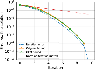
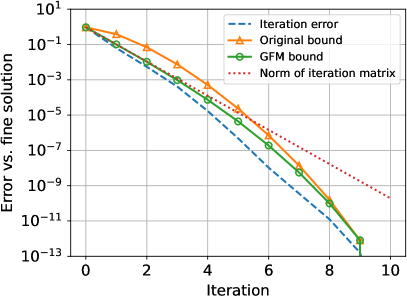
Figure 3: Error bounds for Parareal for (1). Left: $\lambda=i$, right: $\lambda=-1$. Note that for $\lambda=i$, the GFM-bound and the original one are almost identical.

We also plot the linear bound obtained from the $L^{\infty}$ norm of the iteration matrix $\mathbf{R}_{\textsc{Para\-real}}$ defined just after (46). For both values of $\lambda$, the GFM-bounds coincide with the linear bound from $\mathbf{R}_{\textsc{Para\-real}}$ for the first iteration, and the GFM-bound captures the super-linear contraction in later iterations. For $\lambda=i$, the old and new bounds are similar since $\beta$ is close to 1. However, for $\lambda=-1$ where $\beta$ is smaller than one, the new bound gives a sharper estimate of the error, and we can also see that the new bound captures well the transition from the linear to the super-linear convergence regime. On the left in Figure 3, Parareal seems to converge well for imaginary $\lambda=i$. This, however, should not be seen as a working example of Parareal for a hyperbolic type problem, but is rather the effect of the relatively good accuracy of the coarse solver using 20 points per wave length for one wavelength present in the solution time interval we consider. Denoting by $\epsilon_{\Delta}$ the $L_{\infty}$ error with respect to the exact solution, the accuracy of the coarse solver ($\epsilon_{\Delta}=$ 6.22e-01) allows the Parareal error to reach the fine solver error ($\epsilon_{\Delta}=$ 8.16e-07) in $K=8$ iterations. Since the ideal parallel speedup of Parareal, neglecting the coarse solver cost, is bounded by $N/K=1.25$ [1, Sec. 4], this indicates however almost no speedup in practical applications (see also [29]). If we increase the coarse solver error, for instance by multiplying $\lambda$ by a factor $4$ to have now four times more wavelength in the domain, and only 12.5 points per wavelength resolution in the coarse solver, the convergence of Parareal deteriorates massively, as we can see in Figure 4 (left), while this is not the case for the purely negative real fourfold $\lambda=-4$.

This illustrates how Parareal has great convergence difficulties for hyperbolic problems, already well-documented in the literature see e.g. [17, 23]. This is analogous to the difficulties due to the pollution error and damping in multi-grid methods when solving medium to high frequency associated time harmonic problems, see [10, 12, 13, 19, 7] and references therein.

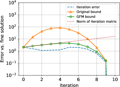
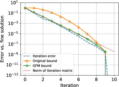
Figure 4: Error bounds for Parareal for (1). Left: $\lambda=4i$, right: $\lambda=-4$.

4 Writing two-level Time Multi-Grid as a block iteration

The idea of time multi-grid (TMG) goes back to the 1980s and 1990s [5, 31, 41]. Furthermore, not long after Parareal was introduced, it was shown to be equivalent to a time multi-grid method, independently of the type of approximation used for the coarse solver [27]. This inspired the development of other time multi-level methods, in particular MGRIT [14]. However, Parareal and MGRIT are usually viewed as iterations acting on values located at the block interface, while TMG-based algorithms, in particular STMG [26], use an iteration updating volume values (i.e. all fine time points in the time domain). In this section, we focus on a generic description of TMG, and show how to write its two-level form applied to the Dahlquist problem as block iteration. In particular, we will show in Section 5 that PFASST can be expressed as a specific variant of TMG. The extension of this analysis to more levels and comparison with multi-level MGRIT is left for future work.

4.1 Definition of a coarse block problem for Time Multi-Grid

To build a coarse problem, we consider a coarsened version of the global problem (12), with a $\mathbf{A}_{C}$ matrix having $N\cdot M^{C}$ rows instead of $N\cdot M$ for $\mathbf{A}$. For each of the $N$ blocks, let $(\tau^{C}_{m})_{1\leq m\leq M^{C}}$ be the normalized $M^{C}$ grid points of a coarser block discretization, with $M^{C}<M$.

We can define a coarse block operator $\bm{\phi}_{C}$ by using the same time integration method as for $\bm{\phi}$ on every block, but with fewer time points. This is equivalent to geometric coarsening used for $h$-multigrid (or geometric multigrid [51]), e.g. when using one time-step of a Runge-Kutta method between each time grid point. It can also be equivalent to spectral coarsening used for $p$-multigrid (or spectral element multigrid [43]), e.g. when one step of a collocation method on $M$ points is used within each block (as for PFASST, see Section 5.3).

We also consider the associated transmission operator $\bm{\chi}_{C}$, and denote by $\bm{u}^{C}_{n}$ the block variable on this coarse time block, which satisfies

(54) $$\bm{\phi}_{C}(\bm{u}^{C}_{1})=\bm{\chi}_{C}\mathbf{T}_{F}^{C}(u_{0}\bm{\mbox{1I}}),\quad\bm{\phi}_{C}\bm{u}^{C}_{n+1}=\bm{\chi}_{C}\bm{u}^{C}_{n}\quad n=1,2,\dots,N-1.$$

Let $\bm{u}^{C}$ be the global coarse variable that solves

(55) $$\mathbf{A}_{C}\bm{u}^{C}:=\begin{pmatrix}\bm{\phi}_{C}&&&\\ -\bm{\chi}_{C}&\bm{\phi}_{C}&&\\ &\ddots&\ddots&\\ &&-\bm{\chi}_{C}&\bm{\phi}_{C}\end{pmatrix}\begin{bmatrix}\bm{u}^{C}_{1}\\ \bm{u}^{C}_{2}\\ \vdots\\ \bm{u}^{C}_{N}\end{bmatrix}=\begin{bmatrix}\bm{\chi}_{C}\mathbf{T}_{F}^{C}(u_{0}\bm{\mbox{1I}})\\ 0\\ \vdots\\ 0\end{bmatrix}=:\bm{f^{C}}.$$

$\mathbf{T}_{F}^{C}$ is a block restriction operator, i.e. a transfer matrix from a fine (F) to a coarse (C) block discretization. Similarly, we have a block prolongation operator $\mathbf{T}_{C}^{F}$, i.e. a transfer matrix from a coarse (C) to a fine (F) block discretization.

Remark 4.1.

While both $\bm{\phi}_{C}$ and $\bm{\tilde{\phi}}$ are approximations of the fine operator $\bm{\phi}$, the main difference between $\bm{\phi}_{C}$ and $\bm{\tilde{\phi}}$ is the size of the vectors they can be applied to ($M^{C}$ and $M$). Furthermore, $\bm{\phi}_{C}$ itself does need the transfer operators $\mathbf{T}_{C}^{F}$ and $\mathbf{T}_{F}^{C}$ to compute approximate values on the fine time points, while $\bm{\tilde{\phi}}$ alone is sufficient (even if it can hide some restriction and interpolation process within). However, the definition of a coarse grid correction in the classical multi-grid formalism needs this separation between transfer and coarse operators (see [51, Sec. 2.2.2]), which limits the use of $\bm{\tilde{\phi}}$ and requires the introduction of $\bm{\phi}_{C}$.

4.2 Block iteration of a Coarse Grid Correction

Let us consider a standalone Coarse Grid Correction (CGC), without pre- or post-smoothing, of a two-level multi-grid iteration [32] applied to (12). One CGC step applied to (12) can be written as

(56) $$\bm{u}^{k+1}=\bm{u}^{k}+\mathbf{\bar{T}}_{C}^{F}\mathbf{A}_{C}^{-1}\mathbf{\bar{T}}_{F}^{C}(\bm{f}-\mathbf{A}\bm{u}^{k}),$$

where $\mathbf{\bar{T}}_{C}^{F}$ denotes the block diagonal matrix formed with $\mathbf{T}_{C}^{F}$ on the diagonal, and similarly for $\mathbf{\bar{T}}_{F}^{C}$. When splitting (56) into two steps,

(57) $$\mathbf{A}_{C}\bm{d}=\mathbf{\bar{T}}_{F}^{C}(\bm{f}-\mathbf{A}\bm{u}^{k}),$$

(58) $$\bm{u}^{k+1}=\bm{u}^{k}+\mathbf{\bar{T}}_{C}^{F}\bm{d},$$

the CGC term (or defect) $\bm{d}$ appears explicitly. Expanding the two steps for $n>0$ into a block formulation and inverting $\bm{\phi}_{C}$ leads to

(59) $$\bm{d}_{n+1} =\bm{\phi}_{C}^{-1}\mathbf{T}_{F}^{C}\bm{\chi}\bm{u}^{k}_{n}-\bm{\phi}_{C}^{-1}\mathbf{T}_{F}^{C}\bm{\phi}\bm{u}^{k}_{n+1}+\bm{\phi}_{C}^{-1}\bm{\chi}_{C}\bm{d}_{n},$$

(60) $$\bm{u}_{n+1}^{k+1} =\bm{u}_{n+1}^{k}+\mathbf{T}_{C}^{F}\bm{d}_{n+1}.$$

Now we need the following simplifying assumption. Prolongation $\mathbf{T}_{C}^{F}$ followed by restriction $\mathbf{T}_{F}^{C}$ leaves the coarse block variables unchanged, i.e.

(61) $$\mathbf{T}_{F}^{C}\mathbf{T}_{C}^{F}=\mathbf{I}.$$

This condition is satisfied in many situations (e.g. restriction with standard injection on a coarse subset of the fine points, or polynomial interpolation with any possible coarse block discretization). Using it in (60) for block index $n$ yields

(62) $$\bm{d}_{n}=\mathbf{T}_{F}^{C}\left(\bm{u}_{n}^{k+1}-\bm{u}_{n}^{k}\right).$$

Inserting $\bm{d}_{n}$ into (59) on the right and the resulting $\bm{d}_{n+1}$ into (60) leads to

(63) $$\bm{u}_{n+1}^{k+1}=(\mathbf{I}-\mathbf{T}_{C}^{F}\bm{\phi}_{C}^{-1}\mathbf{T}_{F}^{C}\bm{\phi})\bm{u}^{k}_{n+1}+\mathbf{T}_{C}^{F}\bm{\phi}_{C}^{-1}\bm{\chi}_{C}\mathbf{T}_{F}^{C}\bm{u}_{n}^{k+1}+\mathbf{T}_{C}^{F}\bm{\phi}_{C}^{-1}\Delta_{\chi}\bm{u}^{k}_{n},$$

with $\Delta_{\chi}:=\mathbf{T}_{F}^{C}\bm{\chi}-\bm{\chi}_{C}\mathbf{T}_{F}^{C}$.

Figure 5: $kn$-graphs for the CGC block iteration, with Assumption 4.2 only (left), and with both Assumptions 4.2 and 4.2 (right).

This is a primary block iteration in the sense of Definition 2.5, and we give its $kn$-graph in Figure 5 (left). We can simplify it further using a second assumption: We consider operators $\mathbf{T}_{F}^{C}$, $\bm{\chi}$ and $\bm{\chi}_{C}$ such that

(64) $$\Delta_{\chi}=\mathbf{T}_{F}^{C}\bm{\chi}-\bm{\chi}_{C}\mathbf{T}_{F}^{C}=0.$$

This holds for classical time-stepping methods when both left and right time sub-interval boundaries are included in the block variables, or for collocation methods using Radau-II or Lobatto type nodes. This last assumption is important to define PFASST (cf. Section 5.3 and see Bolten et al. [3, Remark 1] for more details) and simplifies the analysis of TMG, as both methods use this block iteration. Then, (63) reduces to

(65) $$\bm{u}_{n+1}^{k+1}=(\mathbf{I}-\mathbf{T}_{C}^{F}\bm{\phi}_{C}^{-1}\mathbf{T}_{F}^{C}\bm{\phi})\bm{u}^{k}_{n+1}+\mathbf{T}_{C}^{F}\bm{\phi}_{C}^{-1}\mathbf{T}_{F}^{C}\bm{\chi}\bm{u}_{n}^{k+1}.$$

Again, this is a primary block iteration for which the $kn$-graph is given in Figure 5 (right). It satisfies the consistency condition (14) since $((\mathbf{I}-\mathbf{T}_{C}^{F}\bm{\phi}_{C}^{-1}\mathbf{T}_{F}^{C}\bm{\phi})-\mathbf{I})\bm{\phi}^{-1}\bm{\chi}+\mathbf{T}_{C}^{F}\bm{\phi}_{C}^{-1}\mathbf{T}_{F}^{C}\bm{\chi}=0.$

4.3 Two-level Time Multi-Grid

Gander and Neumüller introduced STMG for discontinuous Galerkin approximations in time [26], which leads to a similar system as (12). We describe the two-level approach for general time discretizations, following their multi-level description [26, Sec. 3]. Consider a coarse problem defined as in Section 4.2 and a damped block Jacobi smoother as in Section 2.2.1 with relaxation parameter $\omega$. Then, a two-level TMG iteration requires the following steps:

1. $\nu_{1}$ pre-relaxation steps (15) with block Jacobi smoother,

2. one CGC (56) inverting the coarse grid operators,

3. $\nu_{2}$ post-relaxation steps (15) with the block Jacobi smoother,

each corresponding to a block iteration. If we combine all these block iterations we do not obtain a primary block iteration but a more complex expression, of which the analysis is beyond the scope of this paper. However, a primary block iteration in the sense of Definition 2.5 is obtained when

• Assumption 4.2 holds, so that $\Delta_{\chi}=0$,

• only one pre-relaxation step is used, $\nu_{1}=1$,

• and no post-relaxation step is considered, $\nu_{2}=0$.

Then, the two-level iteration reduces to the two block updates from (16) and (65),

(66) $$\bm{u}_{n+1}^{k+1/2}=(1-\omega)\bm{u}_{n+1}^{k}+\omega\bm{\phi}^{-1}\bm{\chi}\bm{u}_{n}^{k},$$

(67) $$\bm{u}_{n+1}^{k+1}=\left(\mathbf{I}-\mathbf{T}_{C}^{F}\bm{\phi}_{C}^{-1}\mathbf{T}_{F}^{C}\bm{\phi}\right)\bm{u}^{k+1/2}_{n+1}+\mathbf{T}_{C}^{F}\bm{\phi}_{C}^{-1}\bm{\chi}_{C}\mathbf{T}_{F}^{C}\bm{u}_{n}^{k+1},$$

using $k+1/2$ as intermediate index. Combining (66) and (67) leads to the primary block iteration

(68) $$\bm{u}_{n+1}^{k+1}=\left(\mathbf{I}-\mathbf{T}_{C}^{F}\bm{\phi}_{C}^{-1}\mathbf{T}_{F}^{C}\bm{\phi}\right)\left[(1-\omega)\bm{u}_{n+1}^{k}+\omega\bm{\phi}^{-1}\bm{\chi}\bm{u}_{n}^{k}\right]+\mathbf{T}_{C}^{F}\bm{\phi}_{C}^{-1}\bm{\chi}_{C}\mathbf{T}_{F}^{C}\bm{u}_{n}^{k+1}.$$

If $\omega\neq 1$, all block operators in this primary block iteration are non-zero, and applying Theorem 2.9 leads to the error bound (35). Since the latter is similar to the one obtained for PFASST in Section 5.5.2, we leave its comparison with numerical experiments to Section 5. For $\omega=1$ we get the simplified iteration

(69) $$\bm{u}_{n+1}^{k+1}=\left(\bm{\phi}^{-1}\bm{\chi}-\mathbf{T}_{C}^{F}\bm{\phi}_{C}^{-1}\mathbf{T}_{F}^{C}\bm{\chi}\right)\bm{u}_{n}^{k}+\mathbf{T}_{C}^{F}\bm{\phi}_{C}^{-1}\bm{\chi}_{C}\mathbf{T}_{F}^{C}\bm{u}_{n}^{k+1},$$

and the following result:

Proposition 4.2.

Consider a CGC as in Section 4.2, such that the prolongation and restriction operators (in time) satisfy Assumption 4.2. If Assumption 4.2 also holds and only one block Jacobi pre-relaxation step (15) with $\omega=1$ is used before the CGC, then two-level TMG is equivalent to Parareal, where the coarse solver $\mathcal{G}$ uses the same time integrator as the fine solver $\mathcal{F}$ but with larger time steps, i.e.

(70) $$\mathcal{G}:=\mathbf{T}_{C}^{F}\bm{\phi}_{C}^{-1}\mathbf{T}_{F}^{C}\bm{\chi}.$$

This is a particular case of a result obtained before by Gander [27, Theorem 3.1] but is presented here in the context of our GFM framework and the definition of Parareal given in Section 3.1. In particular, it shows that the simplified two-grid iteration on (12) is equivalent to the preconditioned fixed-point iteration (46) of Parareal if some conditions are met and $\bm{\tilde{\phi}}^{-1}:=\mathbf{T}_{C}^{F}\bm{\phi}_{C}^{-1}\mathbf{T}_{F}^{C}$ is used as the approximate integration operator. However, the TMG iteration here updates also the fine time point values, using $\mathbf{T}_{C}^{F}$ to interpolate the coarse values computed with $\bm{\phi}_{C}$, hence applying the Parareal update to all volume values. This is the only “difference” with the original definition of Parareal in [37], where the update is only applied to the interface value between blocks.

One key idea of STMG that we have not described yet is the block diagonal Jacobi smoother used for relaxation. Even if its diagonal blocks use a time integration operator identical to those of the fine problem (hence requiring the inversion of $\bm{\phi}$), their spatial part in STMG is approximated using one V-cycle multi-grid iteration in space based on a pointwise smoother [26, Sec. 4.3]. We do not cover this aspect in our description of TMG here, since we focus on time only, but describe in the next section a similar approach that is used for PFASST.

5 Writing PFASST as a block iteration

PFASST is also based on a TMG approach using an approximate relaxation step, but the approximation of the block Jacobi smoother is done in time and not in space, in contrast to STMG. In addition, the CGC in PFASST is also approximated, i.e. there is no direct solve on the coarse level to compute the CGC as in STMG. One PFASST iteration is therefore a combination of an Approximate Block Jacobi (ABJ) smoother, see Section 5.2, followed by one (or more) ABGS iteration(s) of Section 2.2.2 on the coarse level to approximate the CGC [11, Sec. 3.2]. While we describe only the two-level variant, the algorithm can use more levels [11, 49]. The main component of PFASST is the approximation of the time integrator blocks using Spectral Deferred Corrections (SDC) [9], from which its other key components (ABJ and ABGS) are built. Hence we first describe how SDC is used to define an ABGS iteration in Section 5.1, then ABJ in Section 5.2, and finally PFASST in Section 5.3.

5.1 Approximate Block Gauss-Seidel with SDC

SDC can be seen as a preconditioner when integrating the ODE problem (1) with collocation methods, see Section 2.1.2. Consider the block operators

(71) $$\bm{\phi}:=(\mathbf{I}-\mathbf{Q}),\quad\bm{\chi}:=\mathbf{H}\quad\Longrightarrow\quad(\mathbf{I}-\mathbf{Q})\bm{u}_{n+1}=\mathbf{H}\bm{u}_{n}.$$

SDC approximates the quadrature matrix $\mathbf{Q}$ by

(72) $$\mathbf{Q}_{\Delta}=\lambda\Delta t\left(\tilde{q}_{m,j}\right),\quad\tilde{q}_{m,j}=\int_{0}^{\tau_{m}}\tilde{l}_{j}(s)ds,$$

where $\tilde{l}_{j}$ is an approximation of the Lagrange polynomial $l_{j}$. Usually, $\mathbf{Q}_{\Delta}$ is lower triangular [46, Sec 3] and easy to invert. This approximation is used to build the preconditioned iteration

(73) $$\bm{u}_{n+1}^{k+1}=\bm{u}_{n+1}^{k}+[\mathbf{I}-\mathbf{Q}_{\Delta}]^{-1}\left(\mathbf{H}\bm{u}_{n}-(\mathbf{I}-\mathbf{Q})\bm{u}_{n+1}^{k}\right)$$

to solve (71), with $\bm{u}_{n+1}$ as unknown. We obtain the generic preconditioned iteration for one block,

(74) $$\bm{u}_{n+1}^{k+1}=\left[\mathbf{I}-\bm{\tilde{\phi}}^{-1}\bm{\phi}\right]\bm{u}_{n+1}^{k}+\bm{\tilde{\phi}}^{-1}\bm{\chi}\bm{u}_{n}\quad\text{with}\quad\bm{\tilde{\phi}}:=\mathbf{I}-\mathbf{Q}_{\Delta}.$$

This shows that SDC inverts the $\bm{\phi}$ operator approximately using $\bm{\tilde{\phi}}$ block by block to solve the global problem (12), i.e. it fixes an $n$ in (74), iterates over $k$ until convergence, and then increments $n$ by one. Hence SDC gives a natural way to define an approximate block integrator $\bm{\tilde{\phi}}$ to be used to build ABJ and ABGS iterations. Defining the ABGS iteration (19) of Section 2.2.2 using the SDC block operators gives the block updating formula

(75) $$\bm{u}_{n+1}^{k+1}=\bm{u}_{n+1}^{k}+[\mathbf{I}-\mathbf{Q}_{\Delta}]^{-1}\left(\mathbf{H}\bm{u}_{n}^{k+1}-(\mathbf{I}-\mathbf{Q})\bm{u}_{n+1}^{k}\right),$$

which we call Block Gauss-Seidel SDC (BGS-SDC), very similar to (73) except that we use the new iterate $\bm{u}_{n}^{k+1}$ and not the converged solution $\bm{u}_{n}$. This is a primary block iteration in the sense of Definition 2.5 with

(76) $$\begin{split}\mathbf{B}^{0}_{1}&:=\mathbf{I}-[\mathbf{I}-\mathbf{Q}_{\Delta}]^{-1}(\mathbf{I}-\mathbf{Q})=[\mathbf{I}-\mathbf{Q}_{\Delta}]^{-1}(\mathbf{Q}-\mathbf{Q}_{\Delta}),\\ \mathbf{B}^{0}_{0}&:=0,\quad\mathbf{B}^{1}_{0}:=[\mathbf{I}-\mathbf{Q}_{\Delta}]^{-1}\mathbf{H},\end{split}$$

and its $kn$-graph is shown in Figure 6 (right).

5.2 Approximate Block Jacobi with SDC

Here we solve the global problem (12) using a preconditioner that can be easily parallelized (Block Jacobi) and combine it with the approximation of the collocation operator $\bm{\phi}$ by $\bm{\tilde{\phi}}$ defined in (71) and (74). This leads to the global preconditioned iteration

(77) $$\bm{u}^{k+1}=\bm{u}^{k}+\mathbf{P}_{Jac}^{-1}(\bm{f}-\mathbf{A}\bm{u}^{k}),\quad\mathbf{P}_{Jac}=\begin{bmatrix}\bm{\tilde{\phi}}&&\\ &\bm{\tilde{\phi}}&\\ &&\ddots\end{bmatrix}.$$

This is equivalent to the block Jacobi relaxation in Section 2.2.1 with $\omega=1$, except that the block operator $\bm{\phi}$ is approximated by $\bm{\tilde{\phi}}$. Using the SDC block operators (71) gives the block updating formula

(78) $$\bm{u}_{n+1}^{k+1}=\bm{u}_{n+1}^{k}+[\mathbf{I}-\mathbf{Q}_{\Delta}]^{-1}\left(\mathbf{H}\bm{u}_{n}^{k}-(\mathbf{I}-\mathbf{Q})\bm{u}_{n+1}^{k}\right),$$

which we call Block Jacobi SDC (BJ-SDC). This is a primary block iteration with

(79) $$\begin{split}\mathbf{B}^{0}_{1}&:=\mathbf{I}-[\mathbf{I}-\mathbf{Q}_{\Delta}]^{-1}(\mathbf{I}-\mathbf{Q})=[\mathbf{I}-\mathbf{Q}_{\Delta}]^{-1}(\mathbf{Q}-\mathbf{Q}_{\Delta}),\\ \mathbf{B}^{0}_{0}&:=[\mathbf{I}-\mathbf{Q}_{\Delta}]^{-1}\mathbf{H},\quad\mathbf{B}^{1}_{0}:=0.\end{split}$$

Its $kn$-graph is shown in Figure 6 (left).

Figure 6: $kn$-graphs for Block Jacobi SDC (left) and Block Gauss-Seidel SDC (right).

This block iteration can be written in the more generic form

(80) $$\bm{u}_{n+1}^{k+1}=\left[\mathbf{I}-\bm{\tilde{\phi}}^{-1}\bm{\phi}\right]\bm{u}_{n+1}^{k}+\bm{\tilde{\phi}}^{-1}\bm{\chi}\bm{u}_{n}^{k}.$$

This is similar to (74) except that we use the current iterate $\bm{u}_{n}^{k}$ from the previous block and not the converged solution $\bm{u}_{n}$. Note that $\bm{\phi}$ and $\bm{\tilde{\phi}}$ do not need to correspond to the SDC operators (71) and (74). This block iteration does not explicitly depend on the use of SDC, hence the name Approximate Block Jacobi (ABJ).

5.3 PFASST

We now give a simplified description of PFASST [11] applied to the Dahlquist problem (1). In particular, this corresponds to doing only one SDC sweep on the coarse level. To write PFASST as a block iteration, we first build the coarse level as in Section 4.2. From that we can form the $\mathbf{\tilde{Q}}$ quadrature matrix associated with the coarse nodes and the coarse matrix $\mathbf{\tilde{H}}$, as we would have done if we were using the collocation method of Section 2.1.2 on the coarse nodes. This leads to the definition of the $\bm{\phi}_{C}$ and $\bm{\chi}_{C}$ operators for the coarse level, combined with the transfer operators $\mathbf{T}_{F}^{C}$ and $\mathbf{T}_{C}^{F}$, from which we can build the global matrices $\mathbf{A}_{C}$, $\mathbf{\bar{T}}_{C}^{F}$ and $\mathbf{\bar{T}}_{F}^{C}$, see Section 4.2. Then we build the two-level PFASST iteration by defining a specific smoother and a modified CGC.

The smoother corresponds to a Block Jacobi SDC iteration (78) from Section 5.2 to produce an intermediate solution

(81) $$\bm{u}_{n+1}^{k+1/2}=[\mathbf{I}-\mathbf{Q}_{\Delta}]^{-1}(\mathbf{Q}-\mathbf{Q}_{\Delta})\bm{u}_{n+1}^{k}+[\mathbf{I}-\mathbf{Q}_{\Delta}]^{-1}\mathbf{H}\bm{u}_{n}^{k},$$

denoted with iteration index $k+1/2$. Using a CGC as in Section 4.2 would provide the global update formula

(82) $$\mathbf{A}_{C}\bm{d}=\mathbf{\bar{T}}_{F}^{C}(\bm{f}-\mathbf{A}\bm{u}^{k+1/2}),$$

(83) $$\bm{u}^{k+1}=\bm{u}^{k+1/2}+\mathbf{\bar{T}}_{C}^{F}\bm{d}.$$

Instead of a direct solve with $\mathbf{A}_{C}$ to compute the defect $\bm{d}$, in PFASST one uses $L$ Block Gauss-Seidel SDC iterations (or sweeps) to approximate it. Then (82) becomes

(84) $$\mathbf{\tilde{P}}_{GS}\bm{d}^{\ell}=(\mathbf{\tilde{P}}_{GS}-\mathbf{A}_{C})\bm{d}^{\ell-1}+\mathbf{\bar{T}}_{F}^{C}(\bm{f}-\mathbf{A}\bm{u}^{k+1/2}),\quad\bm{d}^{0}=0,\quad\ell\in\{1,..,L\},$$

and reduces for one sweep only ($L=1$) to

(85) $$\mathbf{\tilde{P}}_{GS}\bm{d}=\mathbf{\bar{T}}_{F}^{C}(\bm{f}-\mathbf{A}\bm{u}^{k+1/2}),\quad\mathbf{\tilde{P}}_{GS}=\begin{bmatrix}\bm{\tilde{\phi}}_{C}&&\\ -\bm{\chi}_{C}&\bm{\tilde{\phi}}_{C}&\\ &\ddots&\ddots\end{bmatrix}.$$

Here $\mathbf{\tilde{P}}_{GS}$ correspond to the $\mathbf{P}_{GS}$ preconditioning matrix, but written on the coarse level using an SDC-based approximation $\bm{\tilde{\phi}}_{C}$ of the $\bm{\phi}_{C}$ coarse time integrator. Combined with the prolongation on the fine level (83), we get the modified CGC update

(86) $$\bm{u}^{k+1}=\bm{u}^{k+1/2}+\mathbf{\bar{T}}_{C}^{F}\mathbf{\tilde{P}}_{GS}^{-1}\mathbf{\bar{T}}_{F}^{C}(\bm{f}-\mathbf{A}\bm{u}^{k+1/2}),\quad\mathbf{\tilde{P}}_{GS}=\begin{bmatrix}\bm{\tilde{\phi}}_{C}&&\\ -\bm{\chi}_{C}&\bm{\tilde{\phi}}_{C}&\\ &\ddots&\ddots\end{bmatrix},$$

and together with (81) a two level method for the global system (12) [4, Sec. 2.2]. Note that this is the same iteration we obtained for the CGC in Section 4.2, except that the coarse operator $\bm{\phi}_{C}$ has been replaced by $\bm{\tilde{\phi}}_{C}$. Assumption 4.2 holds, since using Lobatto or Radau-II nodes means $\mathbf{H}$ has the form (11), which implies

(87) $$\Delta_{\chi}=\mathbf{T}_{F}^{C}\mathbf{H}-\mathbf{\tilde{H}}\mathbf{T}_{F}^{C}=0.$$

Using similar computations as in Section 4.2 and the block operators defined for collocation and SDC (cf. Section 2.1.2 and Section 5.1) we obtain the block iteration

(88) $$\bm{u}_{n+1}^{k+1}=[\mathbf{I}-\mathbf{T}_{C}^{F}(\mathbf{I}-\mathbf{\tilde{Q}}_{\Delta})^{-1}\mathbf{T}_{F}^{C}(\mathbf{I}-\mathbf{Q})]\bm{u}^{k+1/2}_{n+1}+\mathbf{T}_{C}^{F}(\mathbf{I}-\mathbf{\tilde{Q}}_{\Delta})^{-1}\mathbf{T}_{F}^{C}\mathbf{H}\bm{u}_{n}^{k+1}$$

by substitution into (65). Finally, the combination of the two gives

(89) $$\begin{split}\bm{u}_{n+1}^{k+1}&=[\mathbf{I}-\mathbf{T}_{C}^{F}(\mathbf{I}-\mathbf{\tilde{Q}}_{\Delta})^{-1}\mathbf{T}_{F}^{C}(\mathbf{I}-\mathbf{Q})][\mathbf{I}-\mathbf{Q}_{\Delta}]^{-1}(\mathbf{Q}-\mathbf{Q}_{\Delta})\bm{u}_{n+1}^{k}\\ &~{}+(\mathbf{I}-\mathbf{T}_{C}^{F}[\mathbf{I}-\mathbf{\tilde{Q}}_{\Delta}]^{-1}\mathbf{T}_{F}^{C}(\mathbf{I}-\mathbf{Q}))[\mathbf{I}-\mathbf{Q}_{\Delta}]^{-1}\mathbf{H}\bm{u}_{n}^{k}\\ &~{}+\mathbf{T}_{C}^{F}(\mathbf{I}-\mathbf{\tilde{Q}}_{\Delta})^{-1}\mathbf{T}_{F}^{C}\mathbf{H}\bm{u}_{n}^{k+1}.\end{split}$$

Using the generic formulation with the $\bm{\phi}$ operators gives

(90) $$\begin{split}\bm{u}_{n+1}^{k+1}&=[\mathbf{I}-\mathbf{T}_{C}^{F}\bm{\tilde{\phi}}_{C}^{-1}\mathbf{T}_{F}^{C}\bm{\phi}](\mathbf{I}-\bm{\tilde{\phi}}^{-1}\bm{\phi})\bm{u}_{n+1}^{k}\\ &~{}+(\mathbf{I}-\mathbf{T}_{C}^{F}\bm{\tilde{\phi}}_{C}^{-1}\mathbf{T}_{F}^{C}\bm{\phi})\bm{\tilde{\phi}}^{-1}\bm{\chi}\bm{u}_{n}^{k}+\mathbf{T}_{C}^{F}\bm{\tilde{\phi}}_{C}^{-1}\mathbf{T}_{F}^{C}\bm{\chi}\bm{u}_{n}^{k+1}.\end{split}$$

This is again a primary block iteration in the sense of Definition 2.5, but in contrast to most previously described block iterations, all block operators are non-zero.

5.4 Similarities between PFASST, TMG and Parareal

From the description in the previous section, it is clear that PFASST is very similar to TMG. While TMG uses a (damped) block Jacobi smoother for pre-relaxation and a direct solve for the CGC, PFASST uses instead an approximate Block Jacobi smoother, and solves the CGC using one (or more) ABGS iterations on the coarse grid.

	Block Jacobi ($\omega=1$)	Approximate Block Jacobi
Direct Solver	TMG ($\omega=1$)	TMGf
ABGS (one step)	TMGc	Two-level PFASST

Table 1: Classification of two-level TMG methods, depending on their smoother for fine-level relaxation and computation of the Coarse Grid Correction (CGC).

This interpretation was obtained by Bolten et al. [3, Theorem 1], but is derived here using the GFM framework, and we summarize those differences in Table 1. Changing only the CGC or the smoother in TMG with $\omega=1$ in contrast to both like in PFASST produces two further PinT algorithms. We call those TMG_c (replacing the coarse solver by one step of ABGS) and TMG_f (replacing the fine Block Jacobi solver by ABJ). Note that TMG_c can be interpreted as Parareal using an approximate integration operator and larger time step for the coarse propagator if we set

(91) $$\mathcal{G}:=\mathbf{T}_{C}^{F}\bm{\tilde{\phi}}_{C}^{-1}\mathbf{T}_{F}^{C}\bm{\chi}.$$

Thus, the version of Parareal used in Section 3.2 is equivalent to TMG_c, and differs from PFASST only by the type of smoother used on the fine level.

5.5 Analysis and numerical experiments

5.5.1 Convergence of PFASST iteration components

Since Block Jacobi SDC (78) can be written as a primary block iteration, we can apply Theorem 2.9 with $\beta=0$ to get the error bound

(92) $$e_{n+1}^{k}\leq\begin{cases}\delta(\gamma+\alpha)^{k}\text{ if }k\leq n\\ \displaystyle\delta\gamma^{k}\sum_{i=0}^{n}\binom{k}{i}\left(\frac{\alpha}{\gamma}\right)^{i}\text{ otherwise,}\end{cases}$$

with $\gamma:=\left\lVert[\mathbf{I}-\mathbf{Q}_{\Delta}]^{-1}(\mathbf{Q}-\mathbf{Q}_{\Delta})\right\rVert$, $\alpha:=\left\lVert[\mathbf{I}-\mathbf{Q}_{\Delta}]^{-1}\mathbf{H}\right\rVert$. Note that $\gamma$ is proportional to $\lambda\Delta t$ through the $\mathbf{Q}-\mathbf{Q}_{\Delta}$ term and for small $\Delta t$, $\alpha$ tends to $\left\lVert\mathbf{H}\right\rVert$ which is constant. We can identify two convergence regimes: for early iterations ($k\leq n$), the bound does not contract if $\gamma+\alpha\geq 1$ (which is generally the case). For later iterations ($k>n$), a small-enough time step leads to convergence of the algorithm through the $\gamma^{k}$ factor.

Similarly, for Block Gauss-Seidel SDC (75), Theorem 2.9 with $\alpha=0$ gives

(93) $$e^{k}_{n+1}\leq\delta\frac{\gamma^{k}}{(k-1)!}\sum_{i=0}^{n}\prod_{l=1}^{k-1}(i+l)\beta^{i},$$

where $\gamma:=\left\lVert[\mathbf{I}-\mathbf{Q}_{\Delta}]^{-1}(\mathbf{Q}-\mathbf{Q}_{\Delta})\right\rVert$, $\beta:=\left\lVert[\mathbf{I}-\mathbf{Q}_{\Delta}]^{-1}\mathbf{H}\right\rVert$. This iteration contracts already in early iterations if $\gamma$ is small enough. Since the value for $\gamma$ is the same for both Block Gauss-Seidel SDC and Block Jacobi-SDC, both algorithms have an asymptotically similar convergence rate.

We illustrate this with the following example. Let $\lambda:=i$, $u_{0}:=1$, and let the time interval $[0,\pi]$ be divided into $N=10$ sub-intervals. Inside each sub-interval, we use one step of the collocation method from Section 2.1.2 with $M:=10$ Lobatto-Legendre nodes [28]. This gives us block variables of size $M=10$ and we choose $\mathbf{Q}_{\Delta}$ as the matrix defined by a single Backward Euler step between nodes to build the $\bm{\tilde{\phi}}$ operator. The starting value $\bm{u}^{0}$ for the iteration is initialized with random numbers starting from the same seed. Figure 7 (left) shows the numerical error for the last block using the $L^{\infty}$ norm, the bound obtained with the GFM method and the linear bound using the norm of the global iteration matrix.

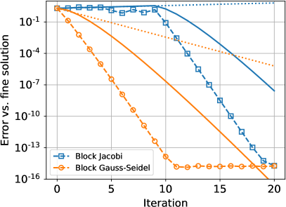
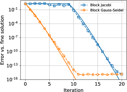
Figure 7: Comparison of numerical errors with GFM-bounds for Block Jacobi SDC and Block Gauss-Seidel SDC. Left: error on the block variables (dashed), GFM-bounds (solid), linear bound from the iteration matrix (dotted). Right: error estimate using the interface approximation from Corollary 2.10. Note that the numerical errors on block variables (left) and at the interface (right) are close but not identical (see Remark 2.12).

As for Parareal in Section 3.2, the GFM-bound is similiar to the iteration matrix bound for the first few iterations, but much tighter for later iterations. In particular, the linear bound cannot show the change in convergence regime of the Block Jacobi SDC iteration (after $k=10$) but the GFM-bound does. Also, we observe that while the GFM-bound overestimates the error, the interface approximation of Corollary 2.10 gives a very good estimate of the error at the interface, see Figure 7 (right).

5.5.2 Analysis and convergence of PFASST

The GFM framework provides directly an error bound for PFASST: applying Theorem 2.9 to (89) gives

(94) $$e_{n+1}^{k}\leq\delta\gamma^{k}\sum_{i=0}^{\min(n,k)}\sum_{l=0}^{n-i}\binom{k}{i}\binom{l+k-1}{l}\left(\frac{\alpha}{\gamma}\right)^{i}\beta^{l},$$

with $\gamma:=||[\mathbf{I}-\mathbf{T}_{C}^{F}(\mathbf{I}-\mathbf{\tilde{Q}}_{\Delta})^{-1}\mathbf{T}_{F}^{C}(\mathbf{I}-\mathbf{Q})][\mathbf{I}-\mathbf{Q}_{\Delta}]^{-1}(\mathbf{Q}-\mathbf{Q}_{\Delta})||$, $\beta:=||\mathbf{T}_{C}^{F}(\mathbf{I}-\mathbf{\tilde{Q}}_{\Delta})^{-1}\mathbf{\tilde{H}}\mathbf{T}_{F}^{C}||$, and $\alpha:=||(\mathbf{I}-\mathbf{T}_{C}^{F}[\mathbf{I}-\mathbf{\tilde{Q}}_{\Delta}]^{-1}\mathbf{T}_{F}^{C}(\mathbf{I}-\mathbf{Q}))[\mathbf{I}-\mathbf{Q}_{\Delta}]^{-1}\mathbf{H}||$.

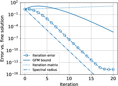
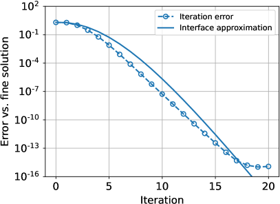
Figure 8: Comparison of numerical errors with GFM-bounds for PFASST. Left: error bound using volume values. Right: estimate using the interface approximation. Note that the numerical errors on block variables (left) and at the interface (right) are very close but not identical (see Remark 2.12).

We compare this bound with numerical experiments. Let $\lambda:=i$, $u_{0}:=1$. The time interval $[0,2\pi]$ for the Dahlquist problem (1) is divided into $N=10$ sub-intervals. Inside each sub-interval we use $M:=6$ Lobatto-Legendre nodes on the fine level and $M^{C}:=2$ Lobatto nodes on the coarse level. The $\mathbf{Q}_{\Delta}$ and $\mathbf{\tilde{Q}}_{\Delta}$ operators use Backward Euler. In Figure 8 (left) we compare the measured numerical error with the GFM-bound and the linear bound from the iteration matrix. As in Section 5.5.1, both bounds overestimate the numerical error, even if the GFM-bound shows convergence for the later iterations, which the linear bound from the iteration matrix cannot. We also added an error estimate built using the spectral radius of the iteration matrix, for which an upper bound was derived in [4]. For this example, the spectral radius reflects the asymptotic convergence rate for the last iterations better than GFM. This highlights a weakness of the current GFM-bound: applying norm and triangle inequalities to the vector error recurrence (25) can induce a large approximation error in the scalar error recurrence (26) that is then solved with generating functions. Improving this is planned for future work.

However, one advantage of the GFM-bound over the spectral radius is its generic aspect allowing it to be applied to many iterative algorithms, even those having an iteration matrix with spectral radius equal to zero like Parareal [45]. Furthermore, the interface approximation from Corollary 2.10 allows us to get a significantly better estimation of the numerical error, as shown in Figure 8 (right). For the GFM-bound we have $(\alpha,\beta,\gamma)=(0.16,1,0.19)$, while for the interface approximation we get $(\bar{\alpha},\bar{\beta},\bar{\gamma})=(0.16,0.84,0.02)$. In the second case, since $\bar{\gamma}$ is one order smaller than the other coefficients, we get an error estimate that is closer to the one for Parareal in Section 3.2 where $\gamma=0$. This similarity between PFASST and Parareal (cf. Section 5.4) will be highlighted in the next section.

6 Comparison of iterative PinT algorithms

Using the notation of the GFM framework, we provide the primary block iterations of all iterative PinT algorithm investigated throughout this paper in Table 2.

Algorithm	$\mathbf{B}_{1}^{0}$ ($\bm{u}_{n+1}^{k}$)	$\mathbf{B}_{0}^{0}$ ($\bm{u}_{n}^{k}$)	$\mathbf{B}_{0}^{1}$ ($\bm{u}_{n}^{k+1}$)
damped Block Jacobi	$\mathbf{I}-\omega\mathbf{I}$	$\omega\bm{\phi}^{-1}\bm{\chi}$	–
ABJ	$\mathbf{I}-\bm{\tilde{\phi}}^{-1}\bm{\phi}$	$\bm{\tilde{\phi}}^{-1}\bm{\chi}$	–
ABGS	$\mathbf{I}-\bm{\tilde{\phi}}^{-1}\bm{\phi}$	–	$\bm{\tilde{\phi}}^{-1}\bm{\chi}$
Parareal	–	$(\bm{\phi}^{-1}-\bm{\tilde{\phi}}^{-1})\bm{\chi}$	$\bm{\tilde{\phi}}^{-1}\bm{\chi}$
TMG	$(1-\omega)(\mathbf{I}-\mathbf{T}_{C}^{F}\bm{\phi}_{C}^{-1}\mathbf{T}_{F}^{C}\bm{\phi})$	$\omega(\bm{\phi}^{-1}-\mathbf{T}_{C}^{F}\bm{\phi}_{C}^{-1}\mathbf{T}_{F}^{C})\bm{\chi}$	$\mathbf{T}_{C}^{F}\bm{\phi}_{C}^{-1}\mathbf{T}_{F}^{C}\bm{\chi}$
TMGc	–	$(\bm{\phi}^{-1}-\mathbf{T}_{C}^{F}\bm{\tilde{\phi}}_{C}^{-1}\mathbf{T}_{F}^{C})\bm{\chi}$	$\mathbf{T}_{C}^{F}\bm{\tilde{\phi}}_{C}^{-1}\mathbf{T}_{F}^{C}\bm{\chi}$
TMGf	$(\mathbf{I}-\mathbf{T}_{C}^{F}\bm{\phi}_{C}^{-1}\mathbf{T}_{F}^{C}\bm{\phi})(\mathbf{I}-\bm{\tilde{\phi}}^{-1}\bm{\phi})$	$(\bm{\tilde{\phi}}^{-1}-\mathbf{T}_{C}^{F}\bm{\phi}_{C}^{-1}\mathbf{T}_{F}^{C}\bm{\phi}\bm{\tilde{\phi}}^{-1})\bm{\chi}$	$\mathbf{T}_{C}^{F}\bm{\phi}_{C}^{-1}\mathbf{T}_{F}^{C}\bm{\chi}$
PFASST	$(\mathbf{I}-\mathbf{T}_{C}^{F}\bm{\tilde{\phi}}_{C}^{-1}\mathbf{T}_{F}^{C}\bm{\phi})(\mathbf{I}-\bm{\tilde{\phi}}^{-1}\bm{\phi})$	$(\bm{\tilde{\phi}}^{-1}-\mathbf{T}_{C}^{F}\bm{\tilde{\phi}}_{C}^{-1}\mathbf{T}_{F}^{C}\bm{\phi}\bm{\tilde{\phi}}^{-1})\bm{\chi}$	$\mathbf{T}_{C}^{F}\bm{\tilde{\phi}}_{C}^{-1}\mathbf{T}_{F}^{C}\bm{\chi}$

Table 2: Summary of all the methods we analyzed, and their block iteration operators. Note that TMG with $\omega=1$ and TMG_c corresponds to Parareal with a specific choice of the coarse propagator.

In particular, the first rows summarize the basic block iterations used as components to build the iterative PinT methods. While damped Block Jacobi (Section 2.2.1) and ABJ (Section 5.2) are more suitable for smoothing, ABGS (Section 2.2.2) is mostly used as solver (e.g. to compute the CGC). This allows us to compare the convergence of each block iteration, and we illustrate this with the following examples.

	$\bm{\phi}^{-1}\bm{\chi}$	$\bm{\tilde{\phi}}^{-1}\bm{\chi}$	$\mathbf{T}_{C}^{F}\bm{\phi}_{C}^{-1}\mathbf{T}_{F}^{C}\bm{\chi}$	$\mathbf{T}_{C}^{F}\bm{\tilde{\phi}}_{C}^{-1}\mathbf{T}_{F}^{C}\bm{\chi}$
Figure 9 (left)	$1.20e^{-5}$	$3.57e^{-1}$	$1.19e^{-2}$	$4.87e^{-1}$
Figure 9 (right)	$3.14e^{-4}$	$6.24e^{-2}$	$5.14e^{-3}$	$2.67e^{-1}$

Table 3: Maximum error over time for each block propagator run sequentially. The first column shows the error of the fine propagator, while the next three columns show the error of the three possible approximate propagators. In the top row, $\bm{\phi}$ corresponds to a collocation method with $M=5$ nodes while $\bm{\phi}_{C}$ is a collocation method with $M=3$ nodes. $\bm{\tilde{\phi}}$ is a backward Euler method with $M=5$ steps per block while $\bm{\tilde{\phi}}_{C}$ is backward Euler with $M=3$ steps per block. In the bottom row, $\bm{\phi}$ corresponds to $M=5$ uniform steps per block of a $4^{th}$ order Runge-Kutta method, $\bm{\phi}_{C}$ is the same method with $M=3$ steps per block. $\bm{\tilde{\phi}}$ is a $2^{nd}$ order Runge-Kutta method (Heun) with $M=5$ uniform steps per block while $\bm{\tilde{\phi}}_{C}$ is the same method with $M=3$ uniform time steps per block.

We consider the Dahlquist problem with $\lambda:=2i-0.2$, $u_{0}=1$. First, we decompose the simulation interval $[0,2\pi]$ into $N=10$ sub-intervals. Next, we choose a block discretization with $M=5$ Lobatto-Legendre nodes, a collocation method on each block for fine integrator $\bm{\phi}$, see Section 2.1.2. We build a coarse block discretization using $M^{C}=3$, and define on each level an approximate integrator using Backward Euler. This allows us to define the $\bm{\tilde{\phi}}$, $\bm{\phi}_{C}$ and $\bm{\tilde{\phi}}_{C}$ integrators, see the legend of Table 3 for more details, where we show the maximum absolute error in time for each of the four propagators run sequentially. The high order collocation method with $M=5$ nodes $\bm{\phi}^{-1}\bm{\chi}$ is the most accurate. The coarse collocation method with $M=3$ nodes interpolated to the fine mesh is still more accurate than the backward Euler method with $M=5$ nodes $\bm{\tilde{\phi}}^{-1}\bm{\chi}$ or the backward Euler method with $M=3$ interpolated to the fine mesh. Then we run all algorithms in Table 2, initializing the block variable iterate with the same random initial guess. The error for the last block variable with respect to the fine sequential solution is shown in Figure 9 (left). In addition, we show the same results in Figure 9 (right), but using the classical $4^{th}$ order Runge-Kutta method as fine propagator, $2^{nd}$ order Runge-Kutta (Heun method) for the approximate integration operator and equidistant points using a volume formulation as described in Section 2.1.1.

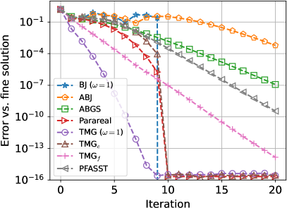
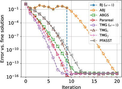
Figure 9: Comparison of iterative methods convergence using the GFM framework. Left: collocation as fine integrator. Right: $4^{th}$ order Runge-Kutta method as fine integrator. Parareal (_ω=1) and Parareal (TMG_c) denote a specific coarse propagator for Parareal.

Note that Parareal, TMG _ω=1 and TMG_c are each Parareal algorithms using respectively $\bm{\tilde{\phi}}^{-1}\bm{\chi}$, $\mathbf{T}_{C}^{F}\bm{\phi}_{C}^{-1}\mathbf{T}_{F}^{C}\bm{\chi}$ and $\mathbf{T}_{C}^{F}\bm{\tilde{\phi}}_{C}^{-1}\mathbf{T}_{F}^{C}\bm{\chi}$ as coarse propagator $\mathcal{G}$ (see Table 3 for their discretization error).

The TMG iteration converges fastest, since it uses the most accurate block integrators on both levels, cf. Table 3. Keeping the same CGC but approximating the smoother, TMG_f improves the first iterations, but convergence for later iterations is closer to PFASST. This suggests that convergence for later iterations is mostly governed by the accuracy of the smoother since both TMG_f and PFASST use ABJ. This is corroborated by the comparison of PFASST and TMG_c, which differ only in their choice of smoother. While the exact Block Jacobi relaxation makes TMG_c converge after $k=N$ iterations (a well known property of Parareal), using the ABJ smoother means that PFASST does not share this property.

On the other hand, the first iterations are also influenced by the CGC accuracy. The iteration error is very similar for PFASST and TMG_c which have the same CGC. This is more pronounced when using the $4^{th}$ order Runge-Kutta method for $\bm{\phi}$, as we see in Figure 9 (right). Early iteration errors are similar for two-level methods that use the same CGC (TMG/ TMG_f, and PFASST/ TMG_c). Similarities of the first iteration errors can also be observed for Parareal and ABGS. Both algorithms use the same $\mathbf{B}_{0}^{1}$ operator, see Table 2. This suggests that early iteration errors are mostly governed by the accuracy of $\mathbf{B}_{0}^{1}$, which is corroborated by the two-level methods (TMG and TMG_f use the same $\mathbf{B}_{0}^{1}$ operator, as PFASST and TMG_c).

Remark 6.1.

An important aspect of this analysis is that it compares only the convergence of each algorithm, and not their overall computational cost. For instance, PFASST and TMG_c appear to be equivalent for the first iterations, but the block iteration of PFASST is cheaper than TMG_c, because an approximate block integrator is used for relaxation. To account for this and build a model for computational efficiency, the GFM framework would need to be combined with a model for computational cost of the different parts in the block iterations. Such a study is beyond the scope of this paper but is the subject of ongoing work.

7 Conclusion

We have shown that the Generating Function Method (GFM) can be used to compare convergence of different iterative PinT algorithms. To do so, we formulated popular methods like Parareal, PFASST, MGRIT or TMG in a common framework based on the definition of a primary block iteration. The GFM analysis showed that all these methods eventually converge super-linearly due to the evolution nature of the problems. We confirmed this by numerical experiments and our Python code is publically available [lunet2023gfm].

Our analysis opens up further research directions. For example, studying multi-step block iterations like MGRIT with FCF-relaxation and more complex two-level methods without Assumption 4.2 would be a useful extension of the GFM framework. Similarly, an extension to multi-level versions of STMG, PFASST and MGRIT would be very valuable. Finally, in practice PinT methods are used to solve space-time problems. The GFM framework should be able to provide convergence bounds in this case as well, potentially even for non-linear problems, considering GFM was used successfully to study Parareal applied to non-linear systems of ODEs [21].

Appendix A Error bounds for Primary Block Iterations

A.1 Incomplete Primary Block Iterations

First, we consider

(95) $$\text{(PBI-1)}:\quad\bm{u}^{k+1}_{n+1} =\mathbf{B}^{1}_{0}\left(\bm{u}^{k+1}_{n}\right)+\mathbf{B}^{0}_{0}\left(\bm{u}^{k}_{n}\right),$$

(96) $$\text{(PBI-2)}:\quad\bm{u}^{k+1}_{n+1} =\mathbf{B}^{0}_{1}(\bm{u}^{k}_{n+1})+\mathbf{B}^{0}_{0}\left(\bm{u}^{k}_{n}\right),$$

(97) $$\text{(PBI-3)}:\quad\bm{u}^{k+1}_{n+1} =\mathbf{B}^{0}_{1}(\bm{u}^{k}_{n+1})+\mathbf{B}^{1}_{0}\left(\bm{u}^{k+1}_{n}\right),$$

where one block operator is zero. (PBI-1) corresponds to Parareal, (PBI-2) to Block Jacobi SDC and (PBI-3) to Block Gauss-Seidel SDC. We recall the notations :

(98) $$\alpha:=\left\lVert\mathbf{B}^{0}_{0}\right\rVert,\quad\beta:=\left\lVert\mathbf{B}^{1}_{0}\right\rVert,\quad\gamma:=\left\lVert\mathbf{B}^{0}_{1}\right\rVert.$$

Application of Lemma 2.7 gives the recurrence relations

(99) $$\text{(PBI-1)}:\quad\rho_{k+1}(\zeta) \leq\frac{\alpha\zeta}{1-\beta\zeta}\rho_{k}(\zeta)\Longrightarrow\rho_{k}(\zeta)\leq\alpha^{k}\left(\frac{\zeta}{1-\beta\zeta}\right)^{k}\rho_{0}(\zeta)$$

(100) $$\text{(PBI-2)}:\quad\rho_{k+1}(\zeta) \leq(\gamma+\alpha\zeta)\rho_{k}(\zeta)\Longrightarrow\rho_{k}(\zeta)\leq\gamma^{k}\left(1+\frac{\alpha}{\gamma}\zeta\right)^{k}\rho_{0}(\zeta)$$

(101) $$\text{(PBI-3)}:\quad\rho_{k+1}(\zeta) \leq\frac{\gamma}{1-\beta\zeta}\rho_{k}(\zeta)\Longrightarrow\rho_{k}(\zeta)\leq\gamma^{k}\frac{1}{(1-\beta\zeta)^{k}}\rho_{0}(\zeta)$$

for the corresponding generating functions. Using definition (30) for $\delta$, we find that $\rho_{0}(\zeta)\leq\delta\sum_{n=0}^{\infty}\zeta^{n+1}.$ By using the binomial series expansion

(102) $$\frac{1}{(1-\beta\zeta)^{k}}=\sum_{n=0}^{\infty}\binom{n+k-1}{n}(\beta\zeta)^{n}$$

for $k>0$ and the Newton binomial sum, we obtain for the three block iterations

(103) $$\text{(PBI-1)}:\quad\rho_{k}(\zeta) \leq\delta\alpha^{k}\zeta\left[\sum_{n=0}^{\infty}\binom{n+k-1}{n}\beta^{n}\zeta^{n+k}\right]\left[\sum_{n=0}^{\infty}\zeta^{n}\right]$$

(104) $$\text{(PBI-2)}:\quad\rho_{k}(\zeta) \leq\delta\gamma^{k}\zeta\left[\sum_{n=0}^{k}\binom{k}{n}\left(\frac{\alpha}{\gamma}\right)^{n}\zeta^{n}\right]\left[\sum_{n=0}^{\infty}\zeta^{n}\right]$$

(105) $$\text{(PBI-3)}:\quad\rho_{k}(\zeta) \leq\delta\gamma^{k}\zeta\left[\sum_{n=0}^{\infty}\binom{n+k-1}{n}\beta^{n}\zeta^{n}\right]\left[\sum_{n=0}^{\infty}\zeta^{n}\right].$$

Error bound for PBI-1

We simplify the expression using

(106) $$\left[\sum_{n=0}^{\infty}\binom{n+k-1}{n}\beta^{n}\zeta^{n+k}\right]=\left[\sum_{n=k}^{\infty}\binom{n-1}{n-k}\beta^{n-k}\zeta^{n}\right],$$

and then the series product formula

(107) $$\left[\sum_{n=0}^{\infty}a_{n}\zeta^{n}\right]\left[\sum_{n=0}^{\infty}b_{n}\zeta^{n}\right]=\sum_{n=0}^{\infty}c_{n}\zeta^{n},\quad c_{n}=\sum_{i=0}^{n}a_{i}b_{n-i},$$

with $b_{n}=1$ and

(108) $$a_{n}=\begin{cases}0\text{ if }n<k,\\ \displaystyle\binom{n-1}{n-k}\beta^{n-k}\text{ otherwise.}\end{cases}$$

From this we get

(109) $$c_{n}=\sum_{i=k}^{n}\binom{i-1}{i-k}\beta^{i-k}=\sum_{i=0}^{n-k}\binom{i+k-1}{i}\beta^{i}=\sum_{i=0}^{n-k}\frac{\prod_{l=1}^{k-1}(i+l)}{(k-1)!}\beta^{i},$$

using the convention that the product reduces to one when there are no terms in it. Identifying coefficients in the power series and rearranging terms yields for $k>0$

(110) $$\boxed{\text{(PBI-1)}:\quad e_{n+1}^{k}\leq\delta\frac{\alpha^{k}}{(k-1)!}\sum_{i=0}^{n-k}\prod_{l=1}^{k-1}(i+l)\beta^{i}.}$$

Following an idea by Gander and Hairer [21], we can also consider the error recurrence $e_{n+1}^{k+1}\leq\alpha e_{n}^{k}+\bar{\beta}e_{n}^{k+1}$, $\bar{\beta}=\max(1,\beta)$. Using the upper bound $\sum_{n=0}^{\infty}\zeta^{n}=\frac{1}{1-\zeta}\leq\frac{1}{1-\bar{\beta}\zeta},$ for the initial error, we avoid the series product and get $\rho_{k}(\zeta)\leq\delta\alpha^{k}\frac{\zeta^{k}}{(1-\bar{\beta})^{k+1}}$ as bound on the generating function. We then obtain the simpler error bound

(111) $$e_{n+1}^{k}\leq\delta\frac{\alpha^{k}}{k!}\bar{\beta}^{n-k}\prod_{l=1}^{k}(n+1-l)$$

as in the proof of [21, Th. 1].

Error bound for PBI-2

We use (107) again with $b_{n}=1$ to get

(112) $$a_{n}=\begin{cases}\displaystyle\binom{k}{n}\left(\frac{\alpha}{\gamma}\right)^{n}\text{ if }n\leq k,\\ 0\text{ otherwise.}\end{cases}$$

From this we get $c_{n}=\sum_{i=0}^{\min(n,k)}\binom{k}{i}\left(\frac{\alpha}{\gamma}\right)^{i},$ which yields for $k>0$ the error bound

(113) $$\boxed{\text{(PBI-2)}:\quad e_{n+1}^{k}\leq\begin{cases}\delta(\gamma+\alpha)^{k}\text{ if }k\leq n,\\ \displaystyle\delta\gamma^{k}\sum_{i=0}^{n}\binom{k}{i}\left(\frac{\alpha}{\gamma}\right)^{i}\text{ otherwise.}\end{cases}}$$

Error bound for PBI-3

We use (107) with $b_{n}=1$ for the series product to get

(114) $$a_{n}=\binom{n+k-1}{n}\beta^{n}=\frac{\prod_{l=1}^{k-1}(n+l)}{(k-1)!}\beta^{n},$$

which yields the error bound

(115) $$\boxed{\text{(PBI-3)}:\quad e^{k}_{n+1}\leq\delta\frac{\gamma^{k}}{(k-1)!}\sum_{i=0}^{n}\prod_{l=1}^{k-1}(i+l)\beta^{i}}$$

for $k>0$.

A.2 Full Primary Block Iteration

We now consider a primary block iteration (13) with all block operators non-zero,

(116) $$\text{(PBI-Full)}:\quad\bm{u}^{k+1}_{n+1}=\mathbf{B}^{0}_{1}\left(\bm{u}^{k}_{n+1}\right)+\mathbf{B}^{1}_{0}\left(\bm{u}^{k+1}_{n}\right)+\mathbf{B}^{0}_{0}\left(\bm{u}^{k}_{n}\right),$$

with $\alpha$, $\beta$ and $\gamma$ defined in (98). Applying Lemma 2.7 leads to

(117) $$\rho_{k+1}(\zeta)\leq\frac{\gamma+\alpha\zeta}{1-\beta\zeta}\rho_{k}(\zeta)\quad\Longrightarrow\quad\rho_{k}(\zeta)\leq\left(\frac{\gamma+\alpha\zeta}{1-\beta\zeta}\right)^{k}\rho_{0}(\zeta).$$

Combining the calculations performed for PBI-2 and PBI-3, we obtain

(118) $$\rho_{k}(\zeta) \leq\delta\zeta\gamma^{k}\left[\sum_{n=0}^{k}\binom{k}{n}\left(\frac{\alpha}{\gamma}\right)^{n}\zeta^{n}\right]\left[\sum_{n=0}^{\infty}\binom{n+k-1}{n}\beta^{n}\zeta^{n}\right]\left[\sum_{n=0}^{\infty}\zeta^{n}\right]$$

(119) $$=\delta\zeta\gamma^{k}\left[\sum_{n=0}^{k}\binom{k}{n}\left(\frac{\alpha}{\gamma}\right)^{n}\zeta^{n}\right]\left[\sum_{n=0}^{\infty}\sum_{i=0}^{n}\binom{i+k-1}{i}\beta^{i}\zeta^{n}\right].$$

Then using (107) with

(120) $$a_{n}=\begin{cases}\displaystyle\binom{k}{n}\left(\frac{\alpha}{\gamma}\right)^{n}\text{ if }n\leq k,\\ 0\text{ otherwise,}\end{cases}\quad b_{n}=\sum_{i=0}^{n}\binom{i+k-1}{i}\beta^{i},$$

we obtain

(121) $$\rho_{k}(\zeta)\leq\delta\zeta\gamma^{k}\sum_{n=0}^{\infty}c_{n}\zeta^{n},\ \mbox{with}\ c_{n}=\sum_{i=0}^{\min(n,k)}\sum_{l=0}^{n-i}\binom{k}{i}\binom{l+k-1}{l}\left(\frac{\alpha}{\gamma}\right)^{i}\beta^{l}.$$

From this we can identify the error bound

(122) $$\boxed{\text{(PBI-Full)}:\quad e_{n+1}^{k}\leq\delta\gamma^{k}\sum_{i=0}^{\min(n,k)}\sum_{l=0}^{n-i}\binom{k}{i}\binom{l+k-1}{l}\left(\frac{\alpha}{\gamma}\right)^{i}\beta^{l}.}$$

References

- [1] E. Aubanel, Scheduling of tasks in the Parareal algorithm, Parallel Comput., 37 (2011), pp. 172–182.
- [2] G. Bal, On the convergence and the stability of the parareal algorithm to solve partial differential equations, in Domain Decomposition Methods in Science and Engineering, R. Kornhuber and et al., eds., vol. 40 of Lecture Notes in Computational Science and Engineering, Berlin, 2005, Springer, pp. 426–432.
- [3] M. Bolten, D. Moser, and R. Speck, A multigrid perspective on the parallel full approximation scheme in space and time, Numerical Linear Algebra with Applications, 24 (2017), p. e2110.
- [4] M. Bolten, D. Moser, and R. Speck, Asymptotic convergence of the parallel full approximation scheme in space and time for linear problems, Numerical linear algebra with applications, 25 (2018), p. e2208.
- [5] J. Burmeister and G. Horton, Time-parallel multigrid solution of the Navier-Stokes equations, in Multigrid methods III, Springer, 1991, pp. 155–166.
- [6] A. J. Christlieb, C. B. Macdonald, and B. W. Ong, Parallel high-order integrators, SIAM J. Sci. Comput., 32 (2010), pp. 818–835.
- [7] P.-H. Cocquet and M. J. Gander, How large a shift is needed in the shifted Helmholtz preconditioner for its effective inversion by multigrid?, SIAM Journal on Scientific Computing, 39 (2017), pp. A438–A478.
- [8] V. Dobrev, T. Kolev, N. Petersson, and J. Schroder, Two-level convergence theory for multigrid reduction in time (MGRIT), tech. report, LLNL-JRNL-692418, 2016.
- [9] A. Dutt, L. Greengard, and V. Rokhlin, Spectral deferred correction methods for ordinary differential equations, BIT, 40 (2000), pp. 241–266.
- [10] H. C. Elman, O. G. Ernst, and D. P. O’leary, A multigrid method enhanced by Krylov subspace iteration for discrete Helmholtz equations, SIAM Journal on scientific computing, 23 (2001), pp. 1291–1315.
- [11] M. Emmett and M. Minion, Toward an efficient parallel in time method for partial differential equations, Comm. App. Math. and Comp. Sci., 7 (2012), pp. 105–132.
- [12] O. G. Ernst and M. J. Gander, Why it is difficult to solve Helmholtz problems with classical iterative methods, in Numerical analysis of multiscale problems, Springer, 2012, pp. 325–363.
- [13] O. G. Ernst and M. J. Gander, Multigrid methods for Helmholtz problems: A convergent scheme in 1d using standard components, Direct and Inverse Problems in Wave Propagation and Applications, 14 (2013).
- [14] R. D. Falgout, S. Friedhoff, T. V. Kolev, S. P. MacLachlan, and J. B. Schroder, Parallel time integration with multigrid, SIAM J. Sci. Comput., 36 (2014), pp. C635–C661.
- [15] C. Farhat and M. Chandesris, Time-decomposed parallel time-integrators: theory and feasibility studies for fluid, structure, and fluid-structure applications, International Journal for Numerical Methods in Engineering, 58 (2003), pp. 1397–1434.
- [16] S. Friedhoff, R. Falgout, T. Kolev, S. MacLachlan, and J. Schroder, A multigrid-in-time algorithm for solving evolution equations in parallel, in Sixteenth Copper Mountain Conference on Multigrid Methods, Copper Mountain, CO, United States, 2013.
- [17] M. J. Gander, Analysis of the Parareal algorithm applied to hyperbolic problems using characteristics, Bol. Soc. Esp. Mat. Apl., 42 (2008), pp. 21–35.
- [18] M. J. Gander, 50 years of time parallel time integration, in Multiple Shooting and Time Domain Decomposition Methods, T. Carraro, M. Geiger, S. Körkel, and R. Rannacher, eds., Springer, 2015, pp. 69–114.
- [19] M. J. Gander, I. G. Graham, and E. A. Spence, Applying GMRES to the Helmholtz equation with shifted Laplacian preconditioning: what is the largest shift for which wavenumber-independent convergence is guaranteed?, Numerische Mathematik, 131 (2015), pp. 567–614.
- [20] M. J. Gander and S. Güttel, ParaExp: A parallel integrator for linear initial-value problems, SIAM J. Sci. Comput., 35 (2013), pp. C123–C142.
- [21] M. J. Gander and E. Hairer, Nonlinear convergence analysis for the Parareal algorithm, in Domain Decomposition Methods in Science and Engineering, Lecture Notes in Computational Science and Engineering, O. B. Widlund and D. E. Keyes, eds., vol. 60, Springer, 2008, pp. 45–56.
- [22] M. J. Gander, F. Kwok, and H. Zhang, Multigrid interpretations of the Parareal algorithm leading to an overlapping variant and MGRIT, Computing and Visualization in Science, 19 (2018), pp. 59–74.
- [23] M. J. Gander and T. Lunet, Toward error estimates for general space-time discretizations of the advection equation, Comput. Vis. Sci., 23 (2020), pp. 1–14.
- [24] M. J. Gander and T. Lunet, ParaStieltjes: Parallel computation of Gauss quadrature rules using a Parareal-like approach for the Stieltjes procedure, Numerical Linear Algebra with Applications, 28 (2021), p. e2314.
- [25] M. J. Gander and T. Lunet, Conservation of difficulties: Parareal for hyperbolic problems and multigrid for Helmholtz, in preparation, (2023).
- [26] M. J. Gander and M. Neumuller, Analysis of a new space-time parallel multigrid algorithm for parabolic problems, SIAM Journal on Scientific Computing, 38 (2016), pp. A2173–A2208.
- [27] M. J. Gander and S. Vandewalle, Analysis of the Parareal time-parallel time-integration method, SIAM J. Sci. Comput., 29 (2007), pp. 556–578.
- [28] W. Gautschi, Orthogonal polynomials: computation and approximation, Oxford University Press, 2004.
- [29] S. Götschel, M. Minion, D. Ruprecht, and R. Speck, Twelve ways to fool the masses when giving parallel-in-time results, in Springer Proceedings in Mathematics & Statistics, Springer International Publishing, 2021, pp. 81–94.
- [30] S. Gunther, L. Ruthotto, J. B. Schroder, E. C. Cyr, and N. R. Gauger, Layer-parallel training of deep residual neural networks, SIAM Journal on Mathematics of Data Science, 2 (2020), pp. 1–23.
- [31] W. Hackbusch, Parabolic multi-grid methods, in Proc. of the sixth int’l. symposium on Computing methods in applied sciences and engineering, VI, North-Holland Publishing Co., 1984, pp. 189–197.
- [32] W. Hackbusch, Multi-grid methods and applications, vol. 4, Springer Science & Business Media, 2013.
- [33] A. Hessenthaler, B. S. Southworth, D. Nordsletten, O. Röhrle, R. D. Falgout, and J. B. Schroder, Multilevel convergence analysis of multigrid-reduction-in-time, SIAM Journal on Scientific Computing, 42 (2020), pp. A771–A796.
- [34] C. Hofer, U. Langer, M. Neumüller, and R. Schneckenleitner, Parallel and robust preconditioning for space-time isogeometric analysis of parabolic evolution problems, SIAM Journal on Scientific Computing, 41 (2019), pp. A1793–A1821.
- [35] D. E. Knuth, The art of computer programming. 1. Fundamental algorithms, Addison-Wesley, 1975.
- [36] M. Lecouvez, R. D. Falgout, C. S. Woodward, and P. Top, A parallel multigrid reduction in time method for power systems, in Power and Energy Society General Meeting (PESGM), 2016, IEEE, 2016, pp. 1–5.
- [37] J.-L. Lions, Y. Maday, and G. Turinici, A ”Parareal” in time discretization of PDE’s, C. R. Math. Acad. Sci. Paris, 332 (2001), pp. 661–668.
- [38] T. Lunet, J. Bodart, S. Gratton, and X. Vasseur, Time-parallel simulation of the decay of homogeneous turbulence using Parareal with spatial coarsening, Computing and Visualization in Science, 19 (2018), pp. 31–44.
- [39] Y. Maday and E. M. Rønquist, Parallelization in time through tensor-product space–time solvers, Comptes Rendus Mathematique, 346 (2008), pp. 113–118.
- [40] M. L. Minion, R. Speck, M. Bolten, M. Emmett, and D. Ruprecht, Interweaving PFASST and parallel multigrid, SIAM J. Sci. Comput., 37 (2015), pp. S244–S263.
- [41] S. Murata, N. Satofuka, and T. Kushiyama, Parabolic multi-grid method for incompressible viscous flows using a group explicit relaxation scheme, Computers & Fluids, 19 (1991), pp. 33–41.
- [42] B. W. Ong and J. B. Schroder, Applications of time parallelization, Computing and Visualization in Science, 23 (2020).
- [43] E. M. Rønquist and A. T. Patera, Spectral element multigrid. i. formulation and numerical results, Journal of Scientific Computing, 2 (1987), pp. 389–406.
- [44] D. Ruprecht, Wave propagation characteristics of parareal, Computing and Visualization in Science, 19 (2018), pp. 1–17.
- [45] D. Ruprecht and R. Krause, Explicit parallel-in-time integration of a linear acoustic-advection system, Comput. & Fluids, 59 (2012), pp. 72–83.
- [46] D. Ruprecht and R. Speck, Spectral deferred corrections with fast-wave slow-wave splitting, SIAM Journal on Scientific Computing, 38 (2016), pp. A2535–A2557.
- [47] M. Schreiber, P. S. Peixoto, T. Haut, and B. Wingate, Beyond spatial scalability limitations with a massively parallel method for linear oscillatory problems, The International Journal of High Performance Computing Applications, 32 (2018), pp. 913–933.
- [48] B. S. Southworth, Necessary conditions and tight two-level convergence bounds for Parareal and multigrid reduction in time, SIAM Journal on Matrix Analysis and Applications, 40 (2019), pp. 564–608.
- [49] R. Speck, D. Ruprecht, R. Krause, M. Emmett, M. L. Minion, M. Winkel, and P. Gibbon, A massively space-time parallel N-body solver, in Proceedings of the International Conference on High Performance Computing, Networking, Storage and Analysis, SC ’12, Los Alamitos, CA, USA, 2012, IEEE Computer Society Press, pp. 92:1–92:11.
- [50] G. A. Staff and E. M. Rønquist, Stability of the Parareal algorithm, in Domain Decomposition Methods in Science and Engineering, Lecture Notes in Computational Science and Engineering, R. Kornhuber and et al, eds., vol. 40, Springer, 2005, pp. 449–456.
- [51] U. Trottenberg, C. W. Oosterlee, and A. Schüller, Multigrid, Academic Press Inc., New-York, 2001.
- [52] G. Wanner and E. Hairer, Solving ordinary differential equations II, Springer Berlin Heidelberg, 1996.