Spatial distribution of HOCN around Sagittarius B2

Abstract

HOCN and HNCO abundance ratio in molecular gas can tell us the information of their formation mechanism. We performed high-sensitivity mapping observations of HOCN, HNCO, and HNC¹⁸O lines around Sagittarius B2 (Sgr B2) with IRAM 30m telescope at 3-mm wavelength. HNCO 4₀₄-3₀₃ and HOCN 4₀₄-3₀₃ are used to obtain the abundance ratio of HNCO to HOCN. The ratio of HNCO 4₀₄-3₀₃ to HNC¹⁸O 4₀₄-3₀₃ is used to calculate the optical depth of HNCO 4₀₄-3₀₃. The abundance ratio of HOCN and HNCO is observed to range from 0.4% to 0.7% toward most positions, which agrees well with the gas-grain model. However, the relative abundance of HOCN is observed to be enhanced toward the direction of Sgr B2 (S), with HOCN to HNCO abundance ratio of $\sim$ 0.9%. The reason for that still needs further investigation. Based on the intensity ratio of HNCO and HNC¹⁸O lines, we updated the isotopic ratio of ¹⁶O/¹⁸O to be 296 $\pm$ 54 in Sgr B2.

1 Introduction

The abundance variation of isomers can give some insights into their formation and destruction (Hollis et al. 2000). The variation can also be used to investigate the environment they exist (Schilke et al. 1992). Thus, obtaining the relative abundances of isomers is of great importance for getting a deeper understanding of a specific isomer family. The combination of HNCO and HOCN can be a good choice to study such astro-chemical effect of isomers (Quan et al. 2010).

HNCO is a very abundant molecule with a peptide-like bond. It was first detected in Sagittarius B2 (hereafter Sgr B2) (OH) (Snyder & Buhl 1972). It was regarded as a tracer of dense gas (Jackson et al. 1984). It was also proposed to be a tracer of interstellar shocks (Zinchenko et al. 2000). Many chemical models were used to reproduce the formation of HNCO, such as gas-phase reaction (Turner et al. 1999) and grain-surface reaction (Garrod et al. 2008). HOCN is the metastable isomer of HNCO. It was also identified in Sgr B2 (OH), with an estimated fractional abundance relative to H₂ of $1\times 10^{-11}$ and an abundance ratio relative to HNCO of 0.5% (Brünken et al. 2009). Then, it was found in other positions towards Sgr B2, including Sgr B2 (M), Sgr B2 (N), and Sgr B2 (S) (Brünken et al. 2010). Quan et al. (2010) used gas-grain models to account for the formation of HNCO and its isomers, including HOCN, in different physical environments. The results show that the formation of HNCO involves both gas-phase reaction and grain-surface reaction.

HNCO was observed to have an expanding ring-like emission in Sgr B2 and the peak position is 2 north of Sgr B2 (M) (Minh & Irvine 2006; Jones et al. 2008), while HOCN were detected in six positions in the Sgr B2 complex (Brünken et al. 2010, 2009). The enhancement of HNCO can be explained by shocks, which release the molecules in the grain mantles into the gas-phase (Minh & Irvine 2006). There is a fairly constant abundance ratio of  0.3%-0.8% between HOCN and HNCO in the six detected positions (Brünken et al. 2010). Therefore, Sgr B2 can be an ideal place to study the relation between HNCO and HOCN. The spatial distribution of HOCN in Sgr B2 and its formation mechanism remain unknown. To further understand the relationship between HNCO and HOCN, mapping observation and extensive surveys in different sources are needed.

In this paper, we present mapping observations of HNCO and HOCN toward Sgr B2 complex. The outline of this article is presented as followed. In Section 2, we describe the observations and data reduction. In Section 3, we give the mapping result, spatial distribution of HNCO $4_{04}-3_{03}$ and HOCN $4_{04}-3_{03}$ emission, and their column density. Scientific discussions are presented in Section 4 and a summary of this paper is given in Section 5.

2 Observations and Data Reduction

We performed point-by-point spectroscopic mapping observations towards Sgr B2 in 2019 May with the IRAM 30m telescope on Pica Veleta, Spain (project 170-18). The observations was performed at 3-mm band. Position-switching mode was adopted. The broad-band Eight MIxer Receiver and the FFTSs in FTS200 mode were used for the observation. The covered frequency range is 82.3-90 GHz, with channel spacing of 0.195 MHz, which corresponds to the velocity resolution of 0.641 km s^-1 at 84 GHz. The telescope pointing was checked every $\sim$ 2 hours on 1757-240. The telescope focus was optimized on 1757-240 at the beginning of the observation. The integration time range from 24 minutes to 98 minutes for different positions, with typical system temperatures of $\sim$ 110K, leading to 1$\sigma$ rms in T${}_{A}^{*}$ of 4-8 mK derived with the line free channels. The antenna temperature ($T_{\rm A}^{\ast}$) was converted to the main beam brightness temperature ($T_{\rm mb}$), using $T_{\rm mb}$=$T_{\rm A}^{\ast}\cdot F_{\rm eff}/B_{\rm eff}$, where the forward efficiency $F_{\rm eff}$ is 0.95 and beam efficiency $B_{\rm eff}$ is 0.81 for 3 mm band.

The observing center is Sgr B2(N) ($\alpha_{J2000}=17^{h}47^{m}20^{s}.0$,$\delta_{J2000}=-28^{\circ}22\arcmin 19.0\arcsec$), with a sampling interval of 30. The off position of ($\delta\alpha$, $\delta\beta$)=(-752, 342) was used (Belloche et al. 2013). HNCO $4_{04}-3_{03}$ at 87925.237 MHz, HNCO $4_{14}-3_{13}$ at 87597.330 MHz, HOCN $4_{04}-3_{03}$ at 83900.570 MHz, and HNC¹⁸O $4_{04}-3_{03}$ at 83191.568 MHz lines within the observing frequency range are used for this study, which are listed in Table 1. The spectroscopic parameters of molecules are taken from CDMS catalog (Müller et al. 2005). $4_{04}-3_{03}$ transition is the strongest for both HNCO and HOCN, which is found to be free of confusion from other species.The data processing was conducted using GILDAS software package, including CLASS and GREG.

Table 1: Transitions of HNCO and HOCN

				Sgr B2(N)		Comments
Molecular	Transition	Rest Freq.	A	$E_{u}$	$\mu^{2}$S
		(MHz)	$\times$ 10-6	(K)	(D2)
HOCN	40,4-30,3	83900.570(0.004)	42.2	10.07	55.212	No blend
HNC18O	40,4-4${}_{0,3},F=3-2$	83191.568(0.030)		9.98	7.332	Partial blend with C13H2CHCN
	40,4-3${}_{0,3},F=5-4$	83191.568(0.030)		9.98	12.546	Partial blend with C13H2CHCN
	40,4-4${}_{0,3},F=4-3$	83191.568(0.030)		9.98	9.623	Partial blend with C13H2CHCN
HNCO	41,4-31,3	87597.330(0.008)	8.04	53.79	9.254	Partial blend with HN13CO
	40,4-30,3	87925.237(0.008)	8.78	10.55	9.986	No blend
	41,3-31,2	88239.020(0.005)	8.22	53.86	9.255	Partial blend with HN13CO

Notes.-: Lines used for mapping. Col. (1): chemical formula; Col. (2): transition quantum numbers (Belloche et al. 2013), Col. (3): rest frequency; Col.(4): emission coefficient A; Col. (5): upper state energy level (K); Col. (6): $\mu^{2}$ is the dipole moment and S is the line strength; Col. (7) comments.

3 Results

We have observed 63 positions toward Sgr B2 to obtain the spatial properties of HNCO and HOCN there. HNCO $4_{04}-3_{03}$ emission was observed to be strong toward all the positions. The emission of HOCN $4_{04}-3_{03}$ was detected to be above 5 $\sigma$ level in 57 positions. The emission of HNC¹⁸O $4_{04}-3_{03}$ was detected to be above 3 $\sigma$ level in 33 positions, while HNCO $4_{14}-3_{13}$ was detected toward 58 positions above 3 $\sigma$ level. The spectra of the lines mentioned above are presented in Figure 1, 2, 3 towards four positions, which are Sgr B2(N), Sgr B2(M), (30, 60), and (60, 60), as examples. The strongest HOCN $4_{04}-3_{03}$ emission comes from (30, 60). From those spectra, we can find that the emission of HNCO $4_{04}-3_{03}$ is about 40 times of HOCN $4_{04}-3_{03}$. No significant line blending for HNC¹⁸O $4_{04}-3_{03}$ at 83191.568 MHz is found, except for that toward Sgr B2(N), which is strongly blended with ¹³CH₂CHCN transitions. The line profile can not be fitted with one simple Gaussian profile for most of the positions, which implies that there are multiple velocity components. To obtain a more accurate value of intensity, we integrate the spectra directly to get the intensity in the later analysis.

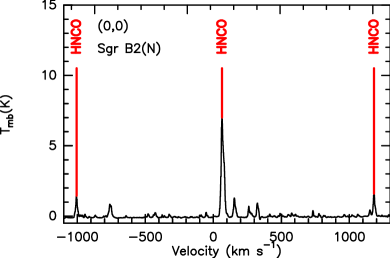
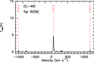
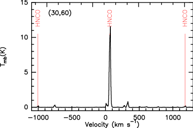
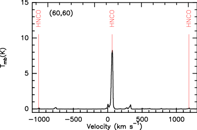
Figure 1: The spectra of HNCO $4_{04}-3_{03}$ toward positions (0,0), (0,-48), (30,60) and (60, 60), corresponding to Sgr B2(N), Sgr B2(M), the strongest emission and other common positions. The red lines mark the place of different transitions.

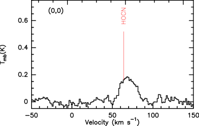
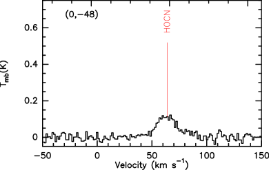
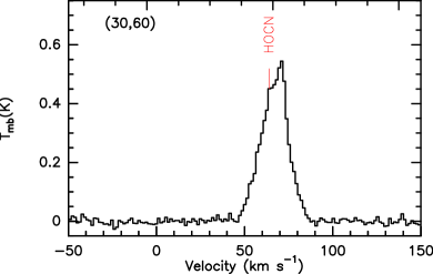
Figure 2: HOCN $4_{04}-3_{03}$ spectra at the rest frequency of 83900.570 MHz toward 4 positions of Sgr B2. The red lines mark the transition of HOCN.

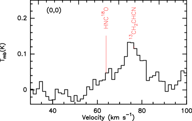
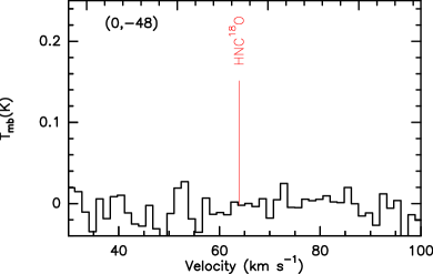
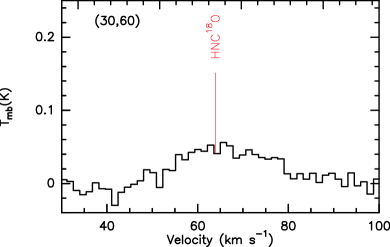
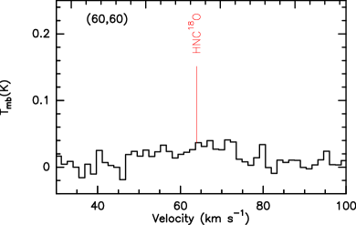
Figure 3: HNC¹⁸O $4_{04}-3_{03}$ spectra at the rest frequency of 83191.568 MHz toward 4 positions of Sgr B2. The red lines correspond to the transition of HNC¹⁸O and the transition of ¹³CH₂CHCN at 83188.122 MHz.

3.1 Spatial distribution of HNCO and HOCN emission

The velocity integrated intensity maps of $4_{04}-3_{03}$, the strongest line for HNCO and HOCN, are presented in Figure 4. In the figure, the positions of Sgr B2 (N) and (M) were marked as $``\times"$. The contour levels range from 20% $\sim$ 90% with the step of 10%. These two maps resemble each other very well. According to the maps, the emission of HNCO $4_{04}-3_{03}$ and HOCN $4_{04}-3_{03}$ are extended with an expanding ring like morphology and peaked at the north of Sgr B2, avoiding the hot cores Sgr B2 (M) and (N), which is similar to the map of HNCO $5_{05}-4_{04}$ emission (Jones et al. 2008).

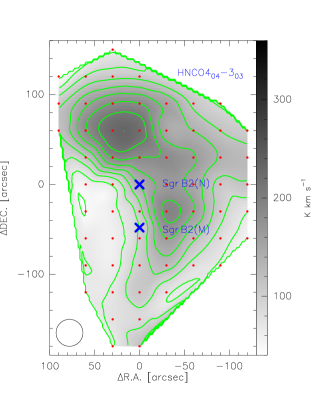
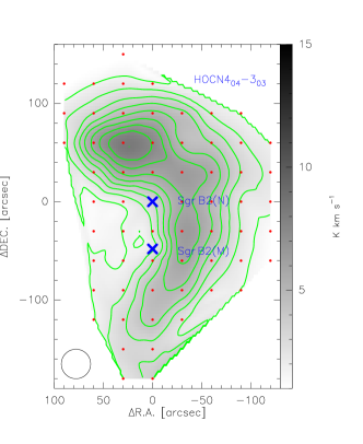
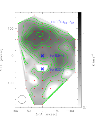
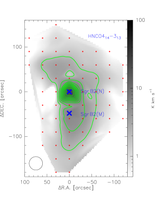
Figure 4: The gray-scale and contours show the integrated emission from HNCO $4_{04}-3_{03}$, HOCN $4_{04}-3_{03}$, HNC¹⁸O $4_{04}-3_{03}$, and HNCO $4_{14}-3_{13}$ in Sgr B2. The contour levels of HNCO $4_{04}-3_{03}$, HOCN $4_{04}-3_{03}$ and HNC¹⁸O $4_{04}-3_{03}$ range from 20% $\sim$ 90% with the step of 10%. To show the structure of HNCO $4_{14}-3_{13}$, the contour levels range from 10% $\sim$ 90% with the step of 10%. The peak values for each panel are 226.3 K km s^-1, 8.1 K km s^-1, 0.66 K km s^-1 and 21.8 K km s^-1 successively. $``\times"$ indicates Sgr B2(N) and Sgr B2(M). The beams are shown in the left corner of each panel.

The velocity integrated intensity maps of HNC¹⁸O $4_{04}-3_{03}$ and HNCO $4_{14}-3_{13}$ are also presented in Figure 4. The profiles of HNC¹⁸O $4_{04}-3_{03}$ are unblended in some positions, in which the intensity of HNC¹⁸O $4_{04}-3_{03}$ can be simply obtained. For the other positions where the profile of HNC¹⁸O and ¹³CH₂CHCN emission can not be distinguished, the intensity of ¹³CH₂CHCN is needed. As the emission of ¹³CH₂CHCN is weak in other positions except for (0,0), the intensity of ¹³CH₂CHCN can be estimated with the line emission of CH₂CHCN. Assuming a constant ratio of ¹³CH₂CHCN and CH₂CHCN in different positions of Sgr B2, with the ratio between ¹³CH₂CHCN and CH₂CHCN lines at position (0,0), the intensity of ¹³CH₂CHCN blended with HNC¹⁸O $4_{04}-3_{03}$ in other positions can be obtained, with a fraction of $\sim 0.3\%$ to HNC¹⁸O $4_{04}-3_{03}$. The emission of HNC¹⁸O is similar to that of HNCO, with an extended spatial distribution. The differences between the maps of isotopes may indicate that the emission of HNCO $4_{04}-3_{03}$ is optically thick in some positions. The emission of HNCO $4_{14}-3_{13}$ is also extended, with two peaks located in the hot cores, Sgr B2 (N) and (M). Considering the larger upper energy ($E_{u}$=53.78 K) of this transition, the two peaks should be mainly caused by the high temperature of the gas there.

3.2 Isotopic ratio ¹⁶O/¹⁸O

Since HN¹³CO lines are strongly blended with the lines of HNCO and OC³⁴S, HNC¹⁸O $4_{04}-3_{03}$ is used to calculate the optical depth of HNCO $4_{04}-3_{03}$. Before using the line ratio of HNC¹⁸O and HNCO $4_{04}-3_{03}$ to obtain the optical depth of HNCO $4_{04}-3_{03}$ at each position, the abundance ratio of HNC¹⁸O and HNCO needs to be known. The line ratio of HNCO and HNC¹⁸O $4_{04}-3_{03}$ can represent the HNCO/HNC¹⁸O abundance ratio in the area where HNCO $4_{04}-3_{03}$ is optically thin. The flux ratio will be the lower limit of the abundance ratio if HNCO $4_{04}-3_{03}$ is not optically thin. To obtain a reliable spectrum of HNC¹⁸O $4_{04}-3_{03}$ with a high signal to noise ratio, averaging data from different positions are needed. The whole region was divided into five parts to avoid position (0,0) where Sgr B2(N) is located and the positions where the emission of HNCO $4_{04}-3_{03}$ is optically thick. The averaged spectra are shown in Figure 5, while the regions used to obtain the averaged spectra are shown in Figure 6.

The integrated flux is used for calculating the line fluxes and ratios, which are presented in Table 2. The averaged ratio is shown in the last column. The flux is integrated with the same velocity range for HNCO $4_{04}-3_{03}$ and HNC¹⁸O $4_{04}-3_{03}$. The red windows in Figure 5 are the velocity ranges used for the integration of both HNCO and HNC¹⁸O $4_{04}-3_{03}$ lines, in order to avoid line blending of HNC¹⁸O from ¹³CH₂CHCN. Assuming that the HNCO/HNC¹⁸O abundance ratio does not vary within Sgr B2, the HNCO/HNC¹⁸O abundance ratio of $\sim$ 296 $\pm$ 54 is a reasonable number. The uncertainty is the square root of the sum of the variance of the HNCO/HNC¹⁸O ratio and the square of the median of ratio error, including the uncertainties of the measurements for the two lines. Assuming that the HNC¹⁸O/HNCO abundance ratio can reflect the isotopic ratio of ¹⁶O/¹⁸O, it will be $\sim$ 296 $\pm$ 54. The result provides a more accurate value of ¹⁶O/¹⁸O ratio than that in the literature (Wannier 1980; Wilson & Rood 1994). It is significantly different from the ratio less than 288 derived with H¹³CO⁺/HC¹⁸O⁺, while it is still within the uncertainty range of 406 $\pm$ 140 derived with ¹³CO/C¹⁸O (Wannier 1980; Wilson & Rood 1994).

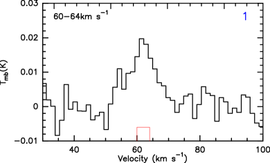
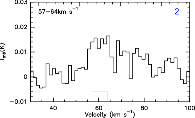
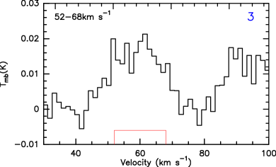
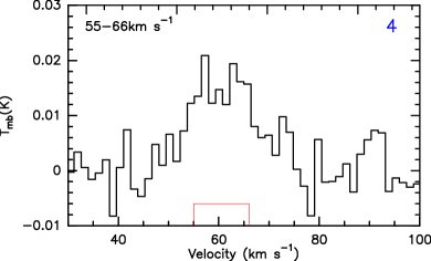
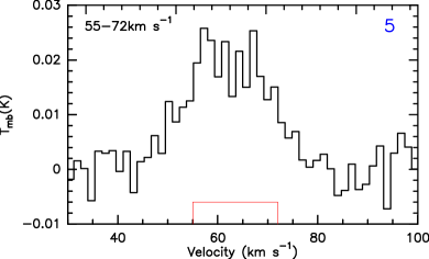
Figure 5: The averaged spectra of HNC¹⁸O. The red windows represent the velocity range used to be integrated.The numbers in the upper right corner represent the position of the region, which is shown in Figure 6.

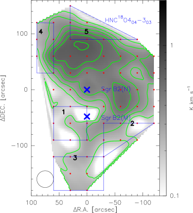
Figure 6: The five regions used to calculate the averaged spectra of HNC¹⁸O.

Table 2: The ratio between ${}^{16}O$ and ${}^{18}O$

	$I_{HNC^{18}O}$	$I_{HNCO}$	R
	$\times$ 10-2 K km s-1	K km s-1
1	6.0(0.77)	14.7(0.039)	245(31)
2	8.4(1.1)	26.1(0.14)	310(41)
3	20.9(2.3)	47.4(0.13)	227(25)
4	14.6(2.5)	48.2(0.064)	330(56)
5	27.6(3.3)	73.9(0.43)	268(32)
average			296(54)

3.3 Optical depth

With the HNCO/HNC¹⁸O abundance ratio, the optical depth of HNCO $4_{04}-3_{03}$ toward different positions can be derived with the intensity ratio of HNCO $4_{04}-3_{03}$ and HNC¹⁸O $4_{04}-3_{03}$. As is mentioned above, the integrated intensity of HNC¹⁸O should be calculated after subtracting the contamination of ¹³CH₂CHCN lines.

When HNCO $4_{04}-3_{03}$ is optically thick, the optical depth can be given by the formulation:

$$\frac{I_{\rm{HNCO}}}{I_{\rm{HNC^{18}O}}}=\frac{1-exp(-\tau)}{(1-exp(-\frac{\tau}{\rm{{}^{16}O/^{18}O}})}$$ (1)

and the $I_{\rm{HNCO}}$ should multiple $\frac{\tau}{1-exp(-\tau)}$ after taking the optical depth into consideration.

For positions with nondetection of HNC¹⁸O emission, optically thin HNCO $4_{04}-3_{03}$ is a reasonable assumption. Therefore, the intensity of HNCO will not be corrected.

3.4 Column densities

The column densities of HNCO and HOCN are calculated assuming local thermodynamic equilibrium (LTE). With the integrated intensity of HNCO, the column density can be given by (Pillai et al. 2007):

$$N=\frac{N_{J}}{g_{J}}\times Q(T_{ex})\times exp(E_{J}/kT_{ex})=\frac{3h}{8\pi^{3}}\times\frac{1}{S\mu^{2}}\times\frac{I_{HNCO}\times Q(T_{ex})}{J_{\nu}(T_{ex})-J_{\nu}(T_{bg})}\times\frac{J(T_{ex})}{\eta_{\nu}}$$ (2)

where $N_{J}$ is the column density of the upper level, $I_{HNCO}$ is the integrated intensity of HNCO after being corrected by the optical depth, $h$ is the Plank constant, $S$ is the line strength, $\mu^{2}$ is the dipole moment, $\eta_{\nu}$ is the beam filling factor, $T_{ex}$ is the excitation temperature, which is equal to the rotation temperature because of the LTE hypothesis, Q(T_ex) is the partition function under the excitation temperature, J(T_ex) is defined as $J(T_{ex})=\frac{exp(E_{u}/kT_{ex})}{exp(h\nu/kT_{ex})-1}$, and J_ν(T) is defined as $J_{\nu}(T)=\frac{h\nu/k}{exp(h\nu/kT_{ex})-1}$. Since HNCO and HOCN emissions are extended, we assume $\eta_{\nu}$ to be 1.

To estimate the dependence of the abundant ratio on the excitation temperature, we calculate the abundance ratio of HNCO to HOCN at positions (0, 60) in different temperatures as an example. As is shown in table 3, the abundance ratio of HOCN to HNCO varies from 0.75% to 0.65% as the temperature varies from 9.375 K to 150 K, which does not change significantly. Since the main goal is to obtain the relative abundance ratio of HOCN to HNCO, 14 K is a reasonable assumption for the excitation temperature.

Table 3: The abundance ratio of HNCO to HOCN under different excitation temperature

Tex	Q(HOCN)	Q(HNCO)	R(NHOCN/NHNCO)
K			%
9.375	20.1244	18.4492	0.65
14	35.4702	30.6393	0.70
18.75	50.8159	42.8291	0.72
37.5	142.1413	117.3039	0.74
75	401.3740	331.9879	0.75
150	1135.3539	943.7057	0.75

Notes. Col(4): the abundance ratio of HOCN to HNCO in position (0,60).

The integrated intensities are calculated using the same velocity ranges. The derived column densities were listed in table 4 and table 5, for those positions where the emission of HOCN is higher than 5 $\sigma$ levels and lower than 5 $\sigma$ levels, respectively. The column density ratios between HNCO and HOCN were listed in the last column. For the positions where HOCN emission is lower than 3 $\sigma$ levels, the upper limits of the intensity and the lower limits of the ratios are given. From the results shown in table 4 and table 5, the ratio of HOCN to HNCO ranges from 0.4% to 0.7% for most of the positions. Some positions located at the south of Sgr B2(S) have the abundance ratio of $\sim$ 0.9%, indicating that the abundance of HOCN is enhanced. From the fourth column of table 4 and table 5, we note that the optical depth of HNCO $4_{04}-3_{03}$ Sgr B2, derived from the ratio of HNCO and HNC¹⁸O, is much smaller than 1, which means the emission of HNCO is almost optically thin in most of the regions of Sgr B2, while there are just a few positions with optically thick HNCO emission. The self-absorption of HNCO lines can be omitted when dealing with the spectra of the whole area.

Table 4: The column density of HNCO and HOCN

ra	dec	$I_{HNCO}$	$\tau$	$I_{HNCO}^{*}$	$N_{HNCO}$	$I_{HOCN}$	$N_{HOCN}$	R
		K km s-1		K km s-1	$\times$ 1015 cm-2	K km s-1	$\times$ 1013 cm-2	%
0	0	163.59(0.81)	0	163.59	2.23	3.92(0.10)	1.14	0.50
60	60	211.89(0.44)	0.26	240.63	3.27	7.15(0.06)	2.08	0.63
-60	60	161.98(0.45)	0.15	174.43	2.37	4.84(0.05)	1.40	0.58
60	-60	75.68(0.32)	0	75.68	1.03	2.04(0.06)	0.59	0.57
-60	-60	140.66(0.98)	0	140.66	1.91	4.38(0.05)	1.27	0.66
30	0	85.05(0.49)	0.14	91.14	1.24	2.30(0.04)	0.67	0.53
-30	0	196.58(1.42)	0	196.58	2.67	6.80(0.04)	1.97	0.73
0	30	216.54(0.55)	0	216.54	2.95	7.06(0.04)	2.05	0.69
0	-30	125.53(0.77)	0	125.53	1.71	3.07(0.04)	0.89	0.51
-30	30	213.91(0.84)	0	213.91	2.91	7.49(0.04)	2.17	0.74
-30	-30	223.97(1.83)	0	223.97	3.05	7.40(0.05)	2.15	0.70
30	30	217.95(0.42)	0	217.95	2.97	7.09(0.04)	2.06	0.68
30	-30	73.33(0.47)	0	73.33	1.00	1.99(0.05)	0.58	0.57
0	60	257.17(0.59)	0	257.17	3.50	8.71(0.05)	2.53	0.71
60	0	66.58(0.44)	0	66.58	0.91	1.62(0.06)	0.47	0.51
-60	0	177.18(1.72)	0	177.18	2.41	5.72(0.05)	1.66	0.68
0	-60	114.15(0.56)	0	114.15	1.55	3.83(0.06)	1.11	0.71
30	60	265.35(0.23)	0.03	269.35	3.66	9.63(0.04)	2.80	0.75
-30	60	175.12(0.29)	0.53	225.61	3.07	5.70(0.05)	1.66	0.53
60	30	132.75(0.51)	0	132.75	1.81	4.00(0.03)	1.16	0.63
-60	30	191.85(1.10)	0.35	227.38	3.09	6.53(0.04)	1.90	0.60
-60	-30	189.09(2.04)	0	189.09	2.57	5.83(0.06)	1.69	0.65
30	-60	68.57(0.28)	0	68.57	0.93	1.95(0.04)	0.57	0.60
-30	-60	188.86(1.26)	0	188.86	2.57	6.93(0.07)	2.01	0.77
-90	0	126.98(1.44)	0	126.98	1.73	2.85(0.05)	0.83	0.47
0	90	216.62(0.31)	0.14	232.14	3.16	6.13(0.04)	1.78	0.56
0	-90	120.38(0.32)	0	120.38	1.64	5.40(0.03)	1.57	0.94
60	90	182.59(0.47)	0	182.59	2.48	3.93(0.07)	1.14	0.44
30	90	217.89(0.24)	0.17	236.94	3.22	5.51(0.06)	1.60	0.49
-30	90	180.20(0.19)	0.09	188.43	2.56	5.12(0.06)	1.49	0.57
-60	90	130.04(0.23)	0	130.04	1.77	2.86(0.05)	0.83	0.46
-90	90	103.41(0.12)	0	103.41	1.41	1.94(0.04)	0.56	0.39
60	-90	81.82(0.13)	0	81.82	1.11	2.11(0.06)	0.61	0.54
30	-90	72.36(0.32)	0	72.36	0.98	2.77(0.04)	0.80	0.81
-30	-90	145.57(0.74)	0	145.57	1.98	5.56(0.05)	1.62	0.80
-60	-90	96.98(0.68)	0	96.98	1.32	2.70(0.05)	0.78	0.59
-90	-90	76.38(0.90)	0	76.38	1.04	1.98(0.05)	0.57	0.54
-90	30	159.60(1.02)	0	159.60	2.17	3.85(0.05)	1.12	0.51

Table 4: $-$ Continued.

ra	dec	$I_{HNCO}$	$\tau$	$I_{HNCO}^{*}$	$N_{HNCO}$	$I_{HOCN}$	$N_{HOCN}$	R
		K km s-1		K km s-1	$\times$ 1015 cm-2	K km s-1	$\times$ 1013 cm-2	%
-90	60	135.04(0.45)	0.05	138.44	1.88	3.10(0.05)	0.90	0.47
-120	0	131.15(0.59)	0	131.15	1.78	2.35(0.05)	0.68	0.38
-120	30	147.17(0.38)	0	147.17	2.00	2.69(0.05)	0.78	0.38
-120	60	119.15(0.20)	0	119.15	1.62	2.20(0.05)	0.64	0.39
-90	-30	118.62(1.73)	0.22	132.15	1.80	2.82(0.05)	0.82	0.45
-90	-60	96.55(1.22)	0	96.55	1.31	2.40(0.05)	0.70	0.52
0	120	126.35(0.22)	0	126.35	1.72	2.21(0.04)	0.64	0.37
30	120	127.80(0.18)	0	127.80	1.74	2.50(0.07)	0.72	0.41
90	90	127.30(0.52)	0	127.30	1.73	2.66(0.08)	0.77	0.44
90	60	134.89(0.64)	0	134.89	1.84	2.67(0.06)	0.77	0.42
90	120	46.97(0.11)	0	46.97	0.64	0.90(0.03)	0.26	0.40
-30	-120	87.69(0.94)	0	87.69	1.19	3.16(0.06)	0.92	0.76
0	-120	126.08(0.42)	0	126.08	1.72	5.13(0.06)	1.49	0.86
30	-120	85.06(0.15)	0	85.06	1.16	3.70(0.05)	1.08	0.92
60	-120	78.10(0.21)	0	78.10	1.06	1.90(0.05)	0.55	0.51
0	-150	100.92(0.35)	0	100.92	1.37	3.68(0.04)	1.07	0.77
30	-150	88.28(0.25)	0	88.28	1.20	3.59(0.06)	1.04	0.86
0	-180	131.58(0.77)	0	131.58	1.79	4.34(0.07)	1.26	0.69
30	-180	78.01(0.27)	0	78.01	1.06	2.98(0.04)	0.87	0.80

Note. Col(1) and Col(2): the equatorial offsets of emission with respect to Sgr B2(N); Col(3): the integrated intensity of HNCO, 1 $\sigma$ level error is given; Col(4): the optical depth of HNCO; Col(5): the integrated intensity of HNCO after considering the optical depth; Col(6): the column density of HNCO; Col(7): the integrated intensity of HOCN, 1 $\sigma$ level error is given; Col(8): the column density of HOCN; Col(9): the abundance ratio of HOCN to HNCO.

Table 5: The column density of HNCO and HOCN

ra	dec	$I_{HNCO}$	$\tau$	$I_{HNCO}^{*}$	$N_{HNCO}$	$I_{HOCN}$	$N_{HNCO}$	R
		K km s-1		K km s-1	$\times$ 1015 cm-2	K km s-1	$\times$ 1013 cm-2	%
-120	-30	82.38(1.10)	0	82.38	1.12	1.38(0.05)	0.40	0.35
60	-30	54.11(0.40)	0	54.11	0.74	1.50(0.05)	0.43	0.58
-120	-60	63.88(0.72)	0	63.88	0.87	1.14(0.05)	0.33	0.37
60	120	110.55(0.25)	0	110.55	1.50	1.93(0.08)	0.56	0.37
30	150	74.51(0.25)	0	74.51	1.01	0.76(0.07)	0.22	0.22
0	-48	110.56(0.64)	0	110.56	1.50	2.76(0.08)	0.80	0.53

Note. The positions shown in table 5 are the area where the emission of HOCN is lower than 5 $\sigma$ levels. Col(1) and Col(2): the equatorial offsets of emission with respect to Sgr B2(N); Col(3): the integrated intensity of HNCO, 1 $\sigma$ level error is given; Col(4): the optical depth of HNCO; Col(5): the integrated intensity of HNCO after considering the optical depth; Col(6): the column density of HNCO; Col(7): the integrated intensity of HOCN, 1 $\sigma$ level error is given; Col(8): the column density of HOCN; Col(9): the abundance ratio of HOCN to HNCO.

4 Discussion

HOCN emission was found to exist in most positions of Sgr B2, confirming that HOCN is also widespread in Sgr B2, just like its isomer specie HNCO. The similarity between the map of HNCO and HOCN emission indicates that they may have common origins. The strong emission discovered in the north of the cloud is likely to be related to the large-scale shock that exists in Sgr B2. The abundance ratio of HOCN to HNCO ranges from 0.4% to 0.7% in most of the positions. The histogram of the abundance ratio of HOCN to HNCO is shown in Figure 7.

4.1 Isotopic ratio

The isotopic ratio of oxygen gained from HNCO and HNC¹⁸O is 296 $\pm$ 54. The assumption used during the calculation is that there is no chemical priority, namely that the ratio of HNCO/HNC¹⁸O can represent the ratio of ¹⁶O/¹⁸O. The validity of the assumption needs to be confirmed, as strong chemical priority will change our result seriously. In addition, the intensity of HNC¹⁸O also plays an important role in the result. As shown in Figure 5, the intensity of HNC¹⁸O after being averaged is just slightly a little bit stronger than 3$\sigma$, while the baseline is hard to be corrected. So the intensities of HNC¹⁸O can not be well determined.

4.2 Abundance ratio of HNCO and HOCN

The abundance ratio of HOCN to HNCO is smaller than 0.4% toward 10 positions, while this value is larger than 0.8% toward 7 positions (see Figure 7). All the 10 positions with extremely low HOCN to HNCO abundance ratio are located in the boundary of this map, with weak HOCN lines which cause large uncertainties of the abundance ratio. On the other hand, the seven positions with the abundance ratios higher than 0.8% located around Sgr B2(S) (marked as red triangles or squares in Figure 8), are with accurate values. The non-detection of HNC¹⁸O $4_{04}-3_{03}$ toward these positions provides small optical depth of HNCO $4_{04}-3_{03}$, which means the underestimation of HNCO is not important. The spectra of HNCO $4_{04}-3_{03}$ and HOCN $4_{04}-3_{03}$ toward positions (0, -90) and (30, -150) are shown in Figure 9 as an example. The high signal to noise ratio ensures that the abundance of HOCN is actually enhanced in these positions, which needs to be explained by new chemical models. The ratios in the rest regions range from 0.4% to 0.7%, without significant variation.

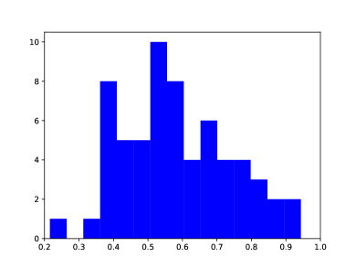
Figure 7: The histogram of the abundance ratios

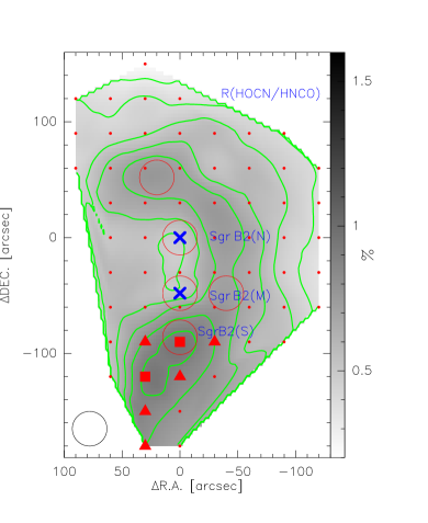
Figure 8: The spatial distribution of HOCN to HNCO ratio. The contour levels range from 30% $\sim$ 100% with the step of 10% and the peak value is 0.94%, while the greyscale is this ratio in percentage. The red triangles and red squares mark the positions where the abundance ratio of HOCN to HNCO is larger than 0.8%. The red squares show the positions with the largest abundance ratio. The red circles represent the positions where Brünken et al. (2010) have observed. The red circle under Sgr B2(M) is Sgr B2 (S).

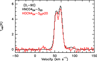
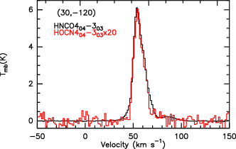
Figure 9: The spectra of HNCO $4_{04}-3_{03}$ and HOCN $4_{04}-3_{03}$ in (0, -90) and (30, -150), marked as red squares in Figure 8.

The strong continuum in Sgr B2(N) and (M) may also have a contribution to the line emission of HNCO. This is ignored to simplify our calculation, so the abundance ratio in Sgr B2(N) and (M) need to be updated in the future.

4.3 Chemical models

The obtained abundance ratios of HOCN/HNCO are about 0.4% to 0.7% in most regions of Sgr B2, implying that the formation mechanism of these two molecules does not vary in different parts of Sgr B2 complex. This result agrees well with the calculated result of the gas-grain model (Quan et al. 2010). In this model, the formation and destruction of both molecules involves gas-phase reactions and grain-surface reactions. HNCO and HOCN initially form on the grain surface, and then they are released from the grain by shocks or some other processes. The fact that the abundance of HOCN is enhanced around Sgr B2(S) needs new chemical models to explain it.

Further observation needs to be conducted to get a more detailed understanding of HNCO and its other isomer in other different sources. It will give us more insights into how the interstellar environment affect the relative abundance of isomer families.

5 Summary

With point-by-point mapping observations of HOCN and HNCO lines around Sgr B2 with IRAM 30m telescope, the spatial distribution of HNCO 4₀₄-3₀₃, HOCN 4₀₄-3₀₃, HNC¹⁸O and HNCO 4₁₄-3₁₃ were obtained. Our main results include:

1. From the spatial distribution of HOCN which is similar to the one of HNCO, we can refer that HOCN is extended in Sgr B2, and perhaps, has a close relationship with HNCO.

2. We note that HOCN molecule is enhanced around Sgr B2(S), with the HOCN to HNCO abundance ratio of $\sim$ 0.9%, while this ratio changes little in the rest positions, ranging from 0.4% to 0.7%. Given the relatively constant abundance ratio of 0.4% to 0.7%, which agrees with the gas-grain model well (Quan et al. 2010), the formation mechanism may be involved both gas-phase reaction and grain-surface reaction, not varying a lot in most parts of Sgr B2.

3. The isotopic ratio of ¹⁶O/¹⁸O derived from the ratio of HNCO/HNC¹⁸O is 296 $\pm$ 54 in Sgr B2. The optical depths of HNCO in most regions of Sgr B2 derived from HNCO/HNC¹⁸O line ratio are smaller than 1, indicating that HNCO 4₀₄-3₀₃ is almost optically thin there.

Whether the condition in Sgr B2 would also apply to other sources may also be a question that needs to be addressed, with further large sample surveys.