Does Configuration Encoding Matter in Learning Software Performance? An Empirical Study on Encoding Schemes

Abstract.

Learning and predicting the performance of a configurable software system helps to provide better quality assurance. One important engineering decision therein is how to encode the configuration into the model built. Despite the presence of different encoding schemes, there is still little understanding of which is better and under what circumstances, as the community often relies on some general beliefs that inform the decision in an ad-hoc manner. To bridge this gap, in this paper, we empirically compared the widely used encoding schemes for software performance learning, namely label, scaled label, and one-hot encoding. The study covers five systems, seven models, and three encoding schemes, leading to 105 cases of investigation.

Our key findings reveal that: (1) conducting trial-and-error to find the best encoding scheme in a case by case manner can be rather expensive, requiring up to 400$+$ hours on some models and systems; (2) the one-hot encoding often leads to the most accurate results while the scaled label encoding is generally weak on accuracy over different models; (3) conversely, the scaled label encoding tends to result in the fastest training time across the models/systems while the one-hot encoding is the slowest; (4) for all models studied, label and scaled label encoding often lead to relatively less biased outcomes between accuracy and training time, but the paired model varies according to the system.

We discuss the actionable suggestions derived from our findings, hoping to provide a better understanding of this topic for the community. To promote open science, the data and code of this work can be publicly accessed at https://github.com/ideas-labo/MSR2022-encoding-study.

1. Introduction

Configurable software systems allow software engineers to tune a set of configurations options (e.g., the cache_size in MongoDB), which can considerably influence their performance, such as latency, runtime and energy consumption, etc. (Chen et al., 2018c; Nair et al., 2020). This is, in fact, a two-edged sword: on one hand, these configuration options offer the flexibility for software to deal with different needs, and even create the foundation to achieve runtime self-adaptation; on the other hand, their combinatorial implications to the performance are often unclear, which may result in severe complication and consequences for software maintenance. For example, Xu et al. (Xu et al., 2015) have discovered that software engineers find it generally difficult to adjust the configurations options in order to adapt the performance.  Han and Yu (Han and Yu, 2016) have further shown that over 59% of the performance bugs nowadays are due to inappropriate configurations. Therefore, to take full advantage of the configurability and adaptability of the software, a performance model, which takes a possible configuration as inputs to predict the likely performance, is of high importance.

Classic performance model has been relying on analytical methods, but soon they become ineffective due primarily to the soaring complexity of modern software systems. In particular, there are two key reasons which prevent the success of analytical methods: (1) analytical models often work on a limited type of configuration options, such as CPU and memory settings (Didona et al., 2015; Chen and Bahsoon, 2017a), which cannot cope with the increasing complexity of modern systems. For example, it has been reported that configurable software systems often contain more complex and diverse types of configuration options that span across different modules, including cache, threading, and parallelism, etc (Xu et al., 2015). (2) Their effectiveness is highly dependent on assumptions about the internal structure and the environment of the software being modeled. However, many modern scenarios, such as cloud-based systems, virtualized and multi-tenant software, intentionally hide such information to promote ease of use, which further reduces the reliability of the analytical methods (Chen, 2019). To overcome the above, machine learning based performance modelings have been gaining momentum in recent years (Kaltenecker et al., 2020), as they require limited assumption, work on arbitrary types of configurations options, and do not rely on heavy human intervention.

A critical engineering decision to make in learning performance for configurable software is how to encode the configurations. In the literature, three encoding schemes are prevalent: (1) embedding the configuration options without scaling (label encoding) (Nair et al., 2020; Siegmund et al., 2015; Nair et al., 2017); (2) doing so with normalization (scaled label encoding) (Chen, 2019; Chen and Bahsoon, 2017a; Ha and Zhang, 2019) or (3) converting them into binary ones that focus on the configuration values of those options, each of which serves as a dimension (one-hot encoding) (Siegmund et al., 2012; Guo et al., 2013; Bao et al., 2019).

Existing work takes one of these three encoding schemes without systematic justification or even discussions, leaving us with little understanding in this regard. This is of concern, as in other domains, such as system security analysis (Jackson and Agrawal, 2019) and medical science (He and Parida, 2016), it has been shown that the encoding scheme chosen can pose significant implications to the success of a machine learning model. Further, choosing one in a trial-and-error manner for each case can be impractical and time-consuming, as we will show in Section 4. It is, therefore, crucial to understand how the encoding performs differently for learning performance of configurable software.

To provide a better understanding of this topic, in this paper, we conduct an empirical study that systematically compares the three encoding schemes for learning software performance and discuss the insights learned. Our hope is to provide more justified understandings towards such an engineering decision in learning software performance under different circumstances.

1.1. Research Questions

Our study covers seven widely used machine learning models for learning software performance, i.e., Decision Tree (DT) (Rokach and Maimon, 2014) (used by (Chen, 2019; Chen and Bahsoon, 2017a; Nair et al., 2020; Guo et al., 2013)), $k$-Nearest Neighbours ($k$NN) (Fix, 1985) (used by  (Kaltenecker et al., 2020)), Kernel Ridge Regression (KRR) (Vovk, 2013) (used by (Kaltenecker et al., 2020)), Linear Regression (LR) (Goldin, 2010) (used by (Chen, 2019; Chen and Bahsoon, 2017a; Siegmund et al., 2012)), Neural Network (NN) (Wang, 2003) (used by (Ha and Zhang, 2019; Fei et al., 2016)), Random Forest (RF) (Ho, 1995) (used by (Valov et al., 2015; Queiroz et al., 2016)), and Support Vector Regression (SVR) (Cortes and Vapnik, 1995) (used by (Chen, 2019; Valov et al., 2015)), together with five popular real-world software systems from prior work (Nair et al., 2020; Peng et al., 2021; Chen and Li, 2021b, a), covering a wide spectrum of characteristics and domains. Naturally, the first research question (RQ) we ask is:

RQ1 seeks to confirm the significance of our study: if it takes an unreasonably long time to conduct trial-and-error in a case-by-case manner, then guidelines on choosing the best encoding scheme under different circumstances become rather important.

What we seek to understand next is:

We use Root Mean Squared Error (RMSE), which is commonly used for software performance modeling (Grohmann et al., 2020; Iorio et al., 2019), as the metric for accuracy. In particular, to make a comparison under the best possible situation, we follow the standard pipeline in software performance learning (Chen, 2019; Chen and Bahsoon, 2017a; Nair et al., 2020; Siegmund et al., 2015; Nair et al., 2017) that tunes the hyperparameters of each model-encoding pair using grid search and cross-validation, which is a common way for parameter tuning (Hinton, 2012).

While prediction accuracy is important, the time taken for training can also become an integral factor in software performance learning. Our next RQ is, therefore:

We examine the training time of each model-encoding pair, including all processes in the learning pipeline such as hyperparameter tuning and validation.

Since it is important to understand the relationship between accuracy and training time, in the final RQ, we ask:

With this, we seek to understand the Pareto-optimal choices that are neither the highest on accuracy nor has the fastest training time (the non-extreme points), especially those that achieve a well-balanced between accuracy and training time, i.e., the knee points.

1.2. Contributions

In a nutshell, we show that choosing the encoding scheme is non-trivial for learning software performance and our key findings are:

• To RQ1: Performing trial-and-error in a case by case manner for finding the best encoding schemes can be rather expensive under some cases, e.g., up to 400$+$ hours.

• To RQ2: The one-hot and label encoding tends to be the best choice while the scaled label encoding performs generally the worst.

• To RQ3: Opposed to RQ2, the scaled label encoding is generally the best choice while the one-hot encoding often exhibit the slowest training.

• To RQ4: Over the models studied, the label and scaled label encoding often lead to less biased results, particularly the latter, but the paired model varies depending on the system.

Deriving from the above, we provide actionable suggestions for learning software performance under a variety of circumstances:

1. When the model to be used involves RF, SVR, KRR, or NN, it is recommended to avoid trial-and-error for finding the best encoding schemes. However, this may be practical for $k$NN, DT, and LR.

2. When the accuracy is of primary concern,

   • using neural network paired with one-hot encoding if all models studied are available to choose.

   • using one-hot encoding for deep learning (NN), lazy models ($k$NN), and kernel models (KRR and SVM).

   • using label encoding for linear (LR) and tree models (DT and RF).

3. When the training time is more important,

   • using linear regression paired with scaled label encoding if all models studied are available to choose.

   • using scaled label encoding for deep learning (NN), linear (LR), and kernel models (KRR and SVR).

   • using label encoding for lazy ($k$NN) and tree models (DT and RF).

4. When a trade-off between accuracy and training time is unclear while an unbiased outcome is preferred,

   • using scaled label encoding for achieving a relatively well-balanced result if considering all models studied, but the paired model requires some efforts to determine.

   • if the model is fixed, only the kernel models (KRR and SVR) and lazy model ($k$NN) have a more balanced outcome achieved by label encoding and scaled label encoding, respectively.

The remaining of this paper is organized as follows: Section 2 introduces the background information. Section 3 elaborates the details of our empirical strategy. Section 4 discusses the results and answers the aforementioned research questions. The insights learned and actionable suggestions are specified in Section 5. Section 6 discusses the implications of our study. Section 7, 8, and 9 present the threats to validity, related work, and conclusion, respectively.

2. Preliminaries

In this section, we elaborate on the necessary background information and the motivation of our study.

2.1. Learning Software Performance

A configurable software system comes with several configuration options, such as the interval for MongoDB. Each of these options can be configured using a set of predefined values, and therefore they are often treated as discrete values, including binary, categorical or numeric options, e.g., we may set $(1,2,3,4)$ on the interval.

Table 1. An example of configurations and performance for MongoDB. $x_{i}$ is the $i$th configuration option and $\varmathbb{P}$ is the performance value (runtime).

$x_{1}$	$x_{2}$	$x_{3}$	$\cdots$	$x_{n-2}$	$x_{n-1}$	$x_{n}$	$\varmathbb{P}$
0	0	0	$\cdots$	0	3	10	1200 seconds
0	1	0	$\cdots$	0	2	11	2100 seconds
$\cdots$	$\cdots$	$\cdots$	$\cdots$	$\cdots$	$\cdots$	$\cdots$	$\cdots$
0	0	1	$\cdots$	0	9	23	1260 seconds
0	0	1	$\cdots$	1	8	65	1140 seconds

Without loss of generality, as shown in Table 1, learning performance for a configurable software often aims to build a regression model that predicts a performance attribute $\varmathbb{P}$ (Chen and Bahsoon, 2017a, 2013; Chen et al., 2014), e.g., runtime, written as:

(1) $$\varmathbb{P}=f(\mathbf{\overline{x}})\text{, }f:\mathbf{\overline{x}}\rightarrow\mathcal{R}$$

whereby $f$ is the actual function learned by a machine learning model; $\mathbf{\overline{x}}$ is the vector that represents a configuration. Given that configurable software runs under an environment, the aim is to train a model that minimizes the generalization error on new configurations which have not been seen in training.

2.2. Encoding Schemes

In machine learning, the steps involved in the automated model building forms a learning pipeline (Mohr et al., 2021). For learning software performance, the standard learning pipeline setting consists of preprocessing, hyperparameter tuning, model training (using all configuration options), and model evaluation (Chen, 2019; Chen and Bahsoon, 2017a; Nair et al., 2020; Siegmund et al., 2015; Nair et al., 2017) (see Section 3 for details).

In all learning pipeline phases, one critical engineering decision, which this paper focuses on, is how the $\mathbf{\overline{x}}$ can be encoded. In general, existing work takes one of the following three encoding schemes:

Label Encoding: This is a widely used scheme (Nair et al., 2020; Siegmund et al., 2015; Nair et al., 2017), where each of the configuration options occupies one dimension in $\mathbf{\overline{x}}$. Taking MongoDB as an example, its configuration can be represented as $\mathbf{\overline{x}}=($cache_size, interval, ssl, data_strategy$)$ where cache_size$=(1,10,10000)$, interval$=(1,2,3,4)$, ssl$=(0,1)$ and data_strategy$=(str\_l1,$ $str\_l2,str\_l3)$. A configuration that is used as a training sample could be $(10000,2,1,1)$, where the data_strategy can be converted into numeric values of $(0,1,2)$.

Scaled Label Encoding: This is a variant of the label encoding used by a state-of-the-art approach (Chen, 2019; Chen and Bahsoon, 2017a; Ha and Zhang, 2019), where each configuration also takes one dimension in $\mathbf{\overline{x}}$. The only difference is that all configurations are normalized to the range between 0 and 1. The same example configuration above for label encoding would be scaled to $(1,\frac{1}{3},1,0.5)$.

One-hot Encoding: Another commonly followed scheme (Siegmund et al., 2012; Guo et al., 2013; Bao et al., 2019) such that each dimension in $\mathbf{\overline{x}}$ refers to the binary form of a particular value for a configuration option. Using the above example of MongoDB, the representation becomes $\mathbf{\overline{x}}=($cache_size_v1, cache_size_v2$,...)$. Each dimension, e.g., cache_size_v1, would have a value of 1 if it is the one that the corresponding configuration chooses, otherwise it is 0. As such, the same configuration $(10000,2,1,1)$ in the label encoding would be represented as $(0,0,1,0,1,0,0,0,1,0,1,0)$ in the one-hot encoding.

Clearly, for binary options, the three encoding methods would be identical, hence in this work, we focus on the systems that also come with complex numeric and categorical configuration options.

2.3. Why Study Them?

Despite the prevalence of the three encoding schemes, existing work often use one of them without justifying their choice for learning software performance (Chen, 2019; Chen and Bahsoon, 2017a; Nair et al., 2020; Siegmund et al., 2015; Nair et al., 2017; Siegmund et al., 2012; Guo et al., 2013; Bao et al., 2019), particularly relating to the accuracy and training time required for the model. Some studies have mentioned the rationals, but a common agreement on which one to use has not yet been drawn. For example, Bao et al. (Bao et al., 2019) state that for categorical configuration options, e.g., cache_mode with three values (memory, disk, mixed), the label encoding unnecessarily assume a natural ordering between the values, as they are represented as $1$, $2$, and $3$. Here, one-hot encoding should be chosen. However, Alaya et al. (Alaya et al., 2019) argue that the one-hot encoding can easily suffer from the multicollinearity issue on categorical configuration options, i.e., it is difficult to handle options interaction. For numeric configuration options, label encoding may fit well, as it naturally comes with order, e.g., the cache_size in MongoDB, which has a set of values $(1,10,10000)$. However, the values, such as the above, can be of largely different scales and thus degrade numeric stability. Indeed, using one-hot encoding could be robust to this issue, but it loses the ordinal property of the numeric configuration option (Siegmund et al., 2015). Similarly, scaled label encoding could reduce the instability and improve the prediction performance (Pan et al., 2016), but it also weakens the interactions between the scaled options and the binary options (as they stay the same). Therefore, there is still no common agreement (or insights) on which encoding scheme to use under what circumstances for learning performance models.

Unlike other domains, software configuration is often highly sparse, leading to unusual data distributions. Specifically, a few configuration options could have large influence on the software performance, while the others are trivial, which makes the decision of encoding scheme difficult. Moreover, it is often the case that we may not fully understand the nature of every configuration option, as the software may be off-the-shelf or close-sourced; hence, one may not be able to choose the right encoding based on purely theoretical understandings. As such, a high-level guideline on choosing the encoding scheme for performance modeling, which gives overall suggestions for the practitioners, is in high demand.

The above thus motivates this empirical study, aiming to analyzing the effectiveness of encoding schemes across various subject systems and machine learning models, summarizing the common behaviors of the encoding methods, and providing actionable advice based on the learning models applied as well as the requirements, e.g., accuracy and training time.

3. Methodology

In this section, we will discuss the methodology and experimental setup of the empirical strategy for our study.

3.1. System and Data Selection

We set the following criteria to select sampled data of configurable systems and their environments when comparing the three encoding schemes:

1. To promote the reproducibility, the systems should be open-sourced and the data should be hosted in public repositories, e.g., GitHub.

2. The system and its environment should have been widely used and tested in existing work.

3. To ensure a case where the encoding schemes can create sufficiently different representations, the system should have at least 10% configuration options that are not categorical/binary.

4. To promote the robustness of our experiments, the subject systems should have different proportions of configuration options that are numerical.

5. To guarantee the scale of the study, we consider systems with more than 5,000 configuration samples.

We shortlisted systems and their data from recent studies on software configuration tuning and modeling (Nair et al., 2020; Peng et al., 2021), from which we identified five systems and their environment according to the above criteria, as shown in Table 2. The five systems contain different percentages of categorical/binary and numeric configuration options while covering five distinct domains.

Note that since the measurement and sampling process for configurable software is usually rather expensive, e.g., Zuluaga et al. (Zuluaga et al., 2013) report that the synthesis of only one software configuration design can take hours or even days, in practice it is not necessarily always possible to gather an extremely large number of data samples. Further, using the full samples for some systems with a large configuration space can easily lead to unrealistic training time for certain models, e.g., with Neural Network, it took several days to complete only one run under our learning pipeline on the full datasets of Trimesh. Therefore in this work, for each system, we randomly sample 5,000 configurations from the dataset as our experiment data, which tends to be reasonable and is also a commonly used setting in previous work (Dorn et al., 2020; Johnsson et al., 2019; Shao et al., 2019; Gerostathopoulos et al., 2018).

Table 2. Datasets of configurable software systems used. $\lvert\mathbfcal{O}\rvert$ (C/N) denotes the number of categorical (including binary) / numerical options.

Dataset	$\lvert\mathbfcal{O}\rvert$ (C/N)	Performance	Description	Used by
MongoDB	14/2	runtime (ms)	NoSQL database	(Peng et al., 2021)
Lrzip	9/3	runtime (ms)	compression tool	(Peng et al., 2021)
Trimesh	9/4	runtime (ms)	triangle meshes library	(Nair et al., 2020; Chen and Li, 2021b)
ExaStencils	4/6	latency (ms)	stencil code generator	(Peng et al., 2021)
x264	4/13	energy (mW)	a video encoder	(Nair et al., 2020; Chen and Li, 2021b)

3.2. Machine Learning Models

In this work, we choose the most common models that are of different types as used in prior studies:

• Linear Model: This type of model build the correlation between configurations options and performance under certain linear assumptions.

  • Linear Regression (LR): A multi-variable linear regression model that linearly correlate the configurations and their options to make prediction. It has been used by (Chen, 2019; Chen and Bahsoon, 2017a; Siegmund et al., 2012). There are three hyperparameters to tune, e.g., n_jobs.

• Deep Learning Model: A model that is based on multiple layers of perceptrons to learn and predict the concepts.

  • Neural Network (NN): A network structure with layers of neurons and connections representing the flow of data. The weights incorporate the influences of each input unit and interactions between them. The NN models have been shown to be successful for modeling software performance, e.g., (Ha and Zhang, 2019; Fei et al., 2016). In this work, we utilize the same network setting and hyperparameter tuning method from the work by Ha and Zhang (Ha and Zhang, 2019).

• Tree Model: This model constructs a tree-like structure with a clear decision boundary on the branches.

  • Decision Tree (DT): A regression tree model that recursively partitions the configurations space to predict the output, which is used by (Chen, 2019; Chen and Bahsoon, 2017a; Nair et al., 2020; Guo et al., 2013). We tune a DT using three hyperparameters, e.g., min_samples_split.

  • Random Forest (RF): An ensemble of decision trees, each of which learns a subset of samples or configurations space. It is a widely used model for performance learning (Valov et al., 2015; Queiroz et al., 2016). There are three hyperparameters to tune, e.g., n_estimators

• Lazy Model: This model delays the learning until the point of prediction.

  • $k$-Nearest Neighbours ($k$NN): A model that considers only already measured neighboring configurations to produce a prediction, which has been commonly used (Kaltenecker et al., 2020). It has four hyperparameters to be tuned, such as n_neighbors.

• Kernel Model: This model performs learning and prediction by means of a kernel function.

  • Kernel Ridge Regression (KRR): A model of kernel transformation that is combined with ridge regression, which is the $L_{2}$-norm regularization. It has been used by (Kaltenecker et al., 2020). There are three hyperparameters to tune, such as alpha.

  • Support Vector Regression (SVR): A model that transforms the configurations space into a higher- dimensional space via the kernel function, as used by (Chen, 2019; Valov et al., 2015). It contains hyperparameters, e.g., kernel_func.

The reasons for the choices are two-fold: (1) they are prominently used in previous work; and (2) they exist standard implementation under the same and widely-used machine learning library, i.e., Sklearn (Pedregosa et al., 2011) and Tensorflow, which reduces the possibility of bias. Note that we did not aim to be exhaustive, but focusing on those that are the most prevalent ones such that the potential impact of this study can be maximized.

3.3. Metrics

Different metrics exist for measuring the accuracy of a prediction model. In this study, we use RMSE because of two reasons: (1) it is a widely used metric for performance modeling of configurable systems in prior work (Grohmann et al., 2020; Iorio et al., 2019); and (2) it has been reported that RMSE can reveal the performance difference better, compared with its popular counterparts such as Mean Relative Error (Chai and Draxler, 2014). RMSE is calculated as:

(2) $$RMSE=\sqrt{\frac{1}{N}\sum_{i=1}^{N}(x_{i}-\hat{x}_{i})^{2}}$$

whereby $x_{i}$ and $\hat{x}_{i}$ are the actual and predicted performance value, respectively; $N$ denotes that total number of testing data samples.

As for the training time, we report the time taken for completing the training process, including hyperparameter tuning and prepossessing as necessary.

3.4. Learning Pipeline Setting

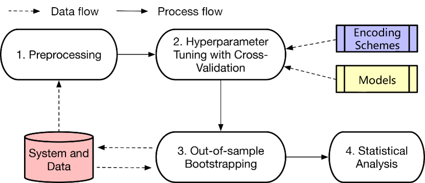
Figure 1. The learning pipeline in this study.

As shown in Figure 1, the standard learning pipeline setting in our empirical study has several key steps as specified below:

1. Preprocessing: For label and one-hot encoding, we utilize the standard encoding functions from the Sklearn library. For the scaled label encoding, we normalize the configurations using the max-min scaling, such that an option value $v$ is standardized as $v={{v-v_{min}}\over{v_{max}-v_{min}}}$, where $v_{max}$ and $v_{min}$ denote the maximum and minimum bound, respectively. In this way, the values of each configuration option can be normalized within the range between $0$ and $1$. We follow the state-of-the-art learning pipeline such that all configuration options and their values are considered in the model  (Chen and Bahsoon, 2017a; Nair et al., 2020; Siegmund et al., 2015; Nair et al., 2017; Bao et al., 2019).

2. Hyperparameter Tuning: It is not uncommon that a model comes with at least one hyperparameter (Li et al., 2020). Therefore, the common practice of the pipeline for learning software performance is to tune them under all encoding schemes (Chen and Bahsoon, 2017a; Nair et al., 2020; Siegmund et al., 2015; Nair et al., 2017; Bao et al., 2019). In this study, we use the GridSearchCV function from Sklearn, which is an exhaustive grid search that evaluates the model quality via 10-fold cross-validation on the training dataset. The one that leads to the best result is used. Note that the default values are always used as a starting point.

3. Bootstrapping: To achieve a reliable conclusion, we conducted out-of-sample bootstrap (without replacement). In particular, we randomly sampled 90% of the data as the training dataset, those samples that were not included in the training were used as the testing samples. The process was repeated 50 times, i.e., there are 50 runs of RMSE (on the testing dataset) and training time to be reported. For each run, all encoding schemes are examined, thereby we ensure that they are evaluated under the same randomly sampled training and testing dataset.

4. Statistical Analysis: To ensure statistical significance in multiple comparisons, we apply Scott-Knott test (Mittas and Angelis, 2013) on all comparisons of over 50 runs and produce a score. In a nutshell, Scott-Knott sorts the list of treatments (the learning model-encoding pairs) by their median RMSE/training time. Next, it splits the list into two sub-lists with the largest expected difference (Xia et al., 2018). Suppose that we compare NN_onehot, RF_onehot, and NN_label, a possible split could be: $\{$NN_onehot, RF_onehot$\}$, $\{$NN_label$\}$, with the score of 2 and 1, respectively. This means that, in the statistical sense, NN_onehot and RF_onehot perform similarly, but they are significantly better than NN_label. Formally, Scott-Knott test aims to find the best split by maximizing the difference $\Delta$ in the expected mean before and after each split:

   (3) $$\Delta=\frac{|l_{1}|}{|l|}(\overline{l_{1}}-\overline{l})^{2}+\frac{|l_{2}|}{|l|}(\overline{l_{2}}-\overline{l})^{2}$$

   whereby $|l_{1}|$ and $|l_{2}|$ are the sizes of two sub-lists ($l_{1}$ and $l_{2}$) from list $l$ with a size $|l|$. $\overline{l_{1}}$, $\overline{l_{2}}$, and $\overline{l}$ denote their mean RMSE/training time values.

   During the splitting, we apply a statistical hypothesis test $H$ to check if $l_{1}$ and $l_{2}$ are significantly different. This is done by using bootstrapping and $\hat{A}_{12}$ (Vargha and Delaney, 2000). If that is the case, Scott-Knott recurses on the splits. In other words, we divide the treatments into different sub-lists if both bootstrap sampling and effect size test suggest that a split is statistically significant (with a confidence level of 99%) and not a small effect ($\hat{A}_{12}\geq 0.6$). The sub-lists are then scored based on their mean RMSE/training time. The higher the score, the better the treatment.

Since there are five systems and environments, together with seven models and three encoding schemes, our empirical study consists of 105 cases of investigation. All the experiments were performed on a Windows 10 server with an Intel Core i5-9400 CPU 2.90GHz and 8GB RAM.

4. Analysis and Results

In this section, we discuss the results of the empirical study with respect to the RQs. All data and code can be accessed at the github repository: https://github.com/ideas-labo/MSR2022-encoding-study.

Table 3. Scott-Knott test, Med (median), and Interquartile Range (IQR) on the RMSE of all models and systems. “onehot”, “label” and “scaled” stand for one-hot, label and scaled label encoding, respectively. A higher score means the RMSE is lower and, therefore, better. For (a) to (e), the pairs are sorted by score, median, and then IQR. For (f), red highlights the best encoding scheme for a model over all systems.

max width = Pair Score Med IQR NN_label 10 2943.38 0.30 max width=.1 NN_scaled 10 2944.45 0.39 max width=.1 NN_onehot 10 2951.74 0.31 max width=.1 KRR_onehot 9 3014.68 0.19 max width=.1 RF_label 8 3019.52 0.20 max width=.1 LR_label 8 3019.55 0.19 max width=.1 RF_scaled 8 3019.63 0.20 max width=.1 LR_onehot 8 3020.36 0.21 max width=.1 KRR_label 8 3024.03 0.19 max width=.1 LR_scaled 8 3026.49 0.19 max width=.1 KRR_scaled 8 3028.21 0.19 max width=.1 RF_onehot 7 3060.11 0.20 max width=.1 DT_scaled 6 3093.12 0.21 max width=.1 DT_onehot 6 3095.11 0.25 max width=.1 DT_label 6 3097.61 0.22 max width=.1 $k$NN_scaled 5 8968.09 1.54 max width=.1 $k$NN_onehot 4 15772.52 0.85 max width=.1 $k$NN_label 3 22114.97 0.99 max width=.1 SVR_onehot 2 41917.30 5.73 max width=.1 SVR_scaled 1 42228.88 5.85 max width=.1 SVR_label 1 42229.54 5.86 max width=.1 Pair Score Med IQR NN_onehot 12 2497.07 0.10 max width=.1 NN_scaled 11 2887.66 0.20 max width=.1 NN_label 10 3019.11 0.34 max width=.1 DT_label 9 15621.69 5.92 max width=.1 DT_scaled 9 15621.77 5.92 max width=.1 RF_scaled 8 25417.20 3.37 max width=.1 RF_label 8 25457.00 3.18 max width=.1 RF_onehot 7 57173.71 5.31 max width=.1 DT_onehot 7 59610.67 9.35 max width=.1 $k$NN_label 6 121668.37 3.96 max width=.1 $k$NN_scaled 5 151716.91 3.54 max width=.1 $k$NN_onehot 4 168726.75 2.81 max width=.1 KRR_onehot 3 192199.55 3.73 max width=.1 LR_onehot 2 193658.25 3.88 max width=.1 LR_scaled 2 194094.27 3.76 max width=.1 KRR_scaled 2 194588.83 3.84 max width=.1 LR_label 2 194648.94 3.79 max width=.1 KRR_label 2 195128.40 3.88 max width=.1 SVR_label 1 321782.26 6.84 max width=.1 SVR_onehot 1 321878.92 6.86 max width=.1 SVR_scaled 1 321923.45 6.86 max width=.1 Pair Score Med IQR NN_scaled 12 398.39 8.37 max width=.1 NN_label 12 398.39 8.37 max width=.1 NN_onehot 11 645.28 9.91 max width=.1 RF_label 10 893.39 9.60 max width=.1 RF_scaled 10 896.18 9.25 max width=.1 RF_onehot 9 947.02 11.43 max width=.1 DT_onehot 8 1104.22 12.32 max width=.1 DT_label 7 1140.59 17.93 max width=.1 DT_scaled 7 1140.63 17.93 max width=.1 $k$NN_onehot 6 1302.37 7.61 max width=.1 $k$NN_scaled 5 1359.37 7.14 max width=.1 KRR_onehot 4 1378.64 8.30 max width=.1 KRR_scaled 3 1410.46 9.14 max width=.1 KRR_label 3 1411.00 9.15 max width=.1 LR_onehot 3 1411.28 10.07 max width=.1 LR_scaled 3 1411.56 9.14 max width=.1 LR_label 3 1412.19 9.08 max width=.1 $k$NN_label 2 1502.74 10.07 max width=.1 SVR_onehot 1 1521.08 11.72 max width=.1 SVR_scaled 1 1525.33 11.75 max width=.1 SVR_label 1 1525.57 11.74 max width=.1 (a). MongoDB (b). Lrzip (c). Trimesh Pair Score Med IQR NN_onehot 14 67.62 0.88 max width=.1 NN_label 13 86.18 0.61 max width=.1 NN_scaled 13 92.37 1.60 max width=.1 RF_scaled 12 158.61 4.00 max width=.1 RF_label 12 159.83 4.00 max width=.1 RF_onehot 12 164.02 3.99 max width=.1 DT_scaled 11 179.07 3.46 max width=.1 DT_label 11 181.96 3.40 max width=.1 DT_onehot 11 182.42 3.42 max width=.1 $k$NN_scaled 10 363.34 2.40 max width=.1 KRR_onehot 10 369.58 0.95 max width=.1 $k$NN_onehot 9 438.83 1.24 max width=.1 $k$NN_label 8 1008.23 1.43 max width=.1 KRR_label 7 1113.89 1.61 max width=.1 SVR_onehot 6 1210.97 1.25 max width=.1 KRR_scaled 5 1306.24 1.56 max width=.1 SVR_label 4 1495.85 1.82 max width=.1 SVR_scaled 3 1507.12 1.92 max width=.1 LR_scaled 2 4562.24 1.97 max width=.1 LR_label 2 4483.84 2.12 max width=.1 LR_onehot 1 7814.81 99 max width=.1 Pair Score Med IQR NN_onehot 19 446.49 7.94 max width=.1 RF_label 19 581.18 6.07 max width=.1 NN_label 18 481.45 6.97 max width=.1 RF_onehot 17 665.35 6.60 max width=.1 NN_scaled 17 671.84 5.32 max width=.1 $k$NN_onehot 16 1021.07 4.49 max width=.1 RF_scaled 15 735.36 4.61 max width=.1 DT_label 14 739.20 6.96 max width=.1 KRR_onehot 13 910.47 4.64 max width=.1 DT_onehot 12 803.96 8.26 max width=.1 DT_scaled 11 950.32 6.04 max width=.1 LR_label 10 1046.27 3.38 max width=.1 $k$NN_scaled 9 939.14 3.79 max width=.1 LR_scaled 8 1084.04 3.01 max width=.1 KRR_label 7 1110.85 3.61 max width=.1 KRR_scaled 6 1183.43 3.39 max width=.1 $k$NN_label 5 1455.11 4.34 max width=.1 SVR_label 4 1487.67 4.93 max width=.1 SVR_onehot 3 1566.62 5.47 max width=.1 SVR_scaled 2 1714.36 5.89 max width=.1 LR_onehot 1 9999.99 17.91 max width=.1 Pair Total Score NN_onehot 66 NN_label 63 NN_scaled 63 RF_onehot 52 RF_label 57 RF_scaled 53 DT_onehot 44 DT_label 47 DT_scaled 44 $k$NN_onehot 39 $k$NN_label 24 $k$NN_scaled 34 LR_onehot 15 LR_label 25 LR_scaled 23 KRR_onehot 39 KRR_label 27 KRR_scaled 24 SVR_onehot 13 SVR_label 11 SVR_scaled 8 (d). ExaStencils (e). x264 (f). Total Scott-Knott scores over all systems

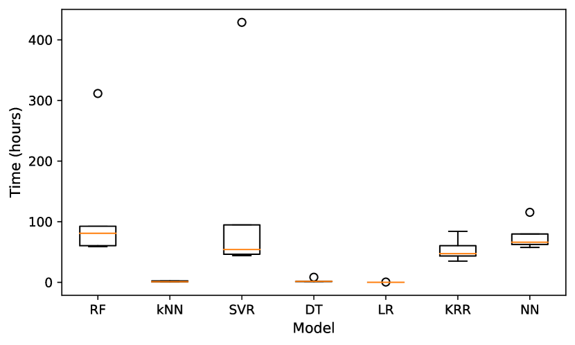
Figure 2. The boxplot of the total time required for identifying the best encoding scheme (with respect to a model) over all systems studied.

4.1. RQ1: Cost of Trial-and-Error

4.1.1. Method

To answer RQ1, for each encoding scheme, we record the time taken to complete all 50 runs under a model and system (including training, hyperparameter tuning, and evaluation). To identify the best encoding scheme using trial-and-error in a case-by-case manner, the “efforts” required would be the total time taken for evaluating a model under all encoding schemes for a system.

Table 4. Scott-Knott test, Med (median), and Interquartile Range (IQR) on the training time (minutes) of all models and systems. The format is the same as that for Table 3.

max width =

Pair Score Med IQR LR_scaled 19 ¡0.01 0.00 max width=.1 LR_label 19 ¡0.01 0.00 max width=.1 LR_onehot 18 0.02 0.01 max width=.1 DT_label 17 0.49 0.01 max width=.1 DT_scaled 16 0.52 0.01 max width=.1 $k$NN_label 15 0.84 0.03 max width=.1 $k$NN_onehot 14 0.86 0.02 max width=.1 DT_onehot 13 1.07 0.04 max width=.1 $k$NN_scaled 12 1.36 0.05 max width=.1 NN_scaled 11 21.61 1.30 max width=.1 NN_onehot 10 23.76 0.20 max width=.1 RF_label 9 28.71 0.33 max width=.1 KRR_scaled 8 28.86 0.08 max width=.1 NN_label 7 29.02 0.24 max width=.1 KRR_onehot 6 29.82 0.08 max width=.1 SVR_label 5 30.45 0.54 max width=.1 RF_scaled 4 34.20 0.62 max width=.1 SVR_onehot 3 34.75 1.61 max width=.1 KRR_label 2 42.28 0.18 max width=.1 RF_onehot 1 47.84 1.62 max width=.1 SVR_scaled 1 60.96 47.97 max width=.1	Pair Score Med IQR LR_scaled 20 ¡0.01 0.00 max width=.1 LR_label 19 ¡0.01 0.00 max width=.1 LR_onehot 18 0.01 0.01 max width=.1 $k$NN_label 17 0.23 0.00 max width=.1 $k$NN_scaled 16 0.30 0.06 max width=.1 DT_scaled 15 0.30 0.01 max width=.1 DT_label 14 0.31 0.01 max width=.1 $k$NN_onehot 13 0.80 0.03 max width=.1 DT_onehot 12 0.85 0.01 max width=.1 KRR_label 11 14.72 0.57 max width=.1 KRR_scaled 10 14.92 0.03 max width=.1 RF_scaled 9 17.01 0.48 max width=.1 RF_label 8 17.15 0.38 max width=.1 SVR_label 7 17.73 0.58 max width=.1 SVR_scaled 6 18.69 0.35 max width=.1 KRR_onehot 5 22.22 1.09 max width=.1 SVR_onehot 4 28.41 0.98 max width=.1 NN_scaled 3 27.85 4.20 max width=.1 NN_label 2 28.03 8.81 max width=.1 NN_onehot 1 35.36 5.16 max width=.1 RF_onehot 1 36.77 0.50 max width=.1	Pair Score Med IQR LR_scaled 20 ¡0.01 0.00 max width=.1 LR_label 20 ¡0.01 0.00 max width=.1 LR_onehot 19 0.01 0.01 max width=.1 $k$NN_label 18 0.17 0.00 max width=.1 $k$NN_scaled 17 0.25 0.02 max width=.1 DT_scaled 16 0.26 0.00 max width=.1 DT_label 15 0.26 0.00 max width=.1 $k$NN_onehot 14 0.47 0.00 max width=.1 DT_onehot 13 1.36 0.03 max width=.1 KRR_label 12 13.78 0.03 max width=.1 KRR_scaled 11 13.75 0.05 max width=.1 KRR_onehot 10 14.35 0.50 max width=.1 RF_scaled 9 16.75 0.15 max width=.1 RF_label 8 16.90 0.27 max width=.1 SVR_scaled 7 17.11 0.04 max width=.1 SVR_label 6 17.33 0.14 max width=.1 SVR_onehot 5 21.01 0.14 max width=.1 NN_label 4 22.25 9.76 max width=.1 NN_scaled 3 23.07 9.06 max width=.1 NN_onehot 2 22.13 10.26 max width=.1 RF_onehot 1 63.34 1.15 max width=.1
(a). MongoDB	(b). Lrzip	(c). Trimesh
Pair Score Med IQR LR_scaled 20 ¡0.01 0.00 max width=.1 LR_label 19 ¡0.01 0.00 max width=.1 LR_onehot 18 0.01 0.00 max width=.1 $k$NN_label 17 0.18 0.00 max width=.1 $k$NN_scaled 16 0.22 0.02 max width=.1 DT_scaled 15 0.23 0.00 max width=.1 DT_label 14 0.26 0.01 max width=.1 $k$NN_onehot 13 0.49 0.05 max width=.1 DT_onehot 12 0.73 0.01 max width=.1 KRR_scaled 11 13.96 0.15 max width=.1 KRR_onehot 10 15.30 2.39 max width=.1 RF_label 9 15.64 0.35 max width=.1 RF_scaled 8 15.86 0.26 max width=.1 SVR_scaled 7 16.98 0.10 max width=.1 SVR_label 6 16.48 3.21 max width=.1 NN_onehot 5 18.02 4.46 max width=.1 SVR_onehot 5 18.50 0.07 max width=.1 KRR_label 4 21.01 21.64 max width=.1 NN_scaled 3 25.70 19.07 max width=.1 NN_label 2 29.11 24.35 max width=.1 RF_onehot 1 32.51 44.27 max width=.1	Pair Score Med IQR LR_label 19 ¡0.01 0.00 max width=.1 LR_scaled 18 ¡0.01 0.00 max width=.1 DT_label 17 0.41 0.00 max width=.1 $k$NN_label 16 0.46 0.00 max width=.1 DT_scaled 15 0.48 0.00 max width=.1 $k$NN_scaled 14 0.48 0.01 max width=.1 LR_onehot 13 0.57 0.02 max width=.1 $k$NN_onehot 12 1.98 0.04 max width=.1 DT_onehot 11 9.17 0.05 max width=.1 KRR_label 10 18.87 0.88 max width=.1 SVR_scaled 9 19.69 0.42 max width=.1 NN_scaled 8 16.83 0.82 max width=.1 KRR_onehot 7 23.76 0.21 max width=.1 KRR_scaled 6 33.79 0.33 max width=.1 NN_label 5 29.38 2.17 max width=.1 RF_scaled 5 30.28 0.07 max width=.1 SVR_label 5 35.82 0.15 max width=.1 RF_label 4 34.27 3.76 max width=.1 NN_onehot 3 81.93 4.25 max width=.1 RF_onehot 2 244.98 10.31 max width=.1 SVR_onehot 1 519.99 23.35 max width=.1	Pair Score LR_onehot 86 LR_label 96 LR_scaled 97 $k$NN_onehot 66 $k$NN_label 83 $k$NN_scaled 75 DT_onehot 61 DT_label 77 DT_scaled 77 KRR_onehot 38 KRR_label 39 KRR_scaled 46 SVR_onehot 18 SVR_label 29 SVR_scaled 30 RF_onehot 6 RF_label 38 RF_scaled 35 NN_onehot 21 NN_label 20 NN_scaled 28
(d). ExaStencils	(e). x264	(f). Total Scott-Knott scores over all systems

4.1.2. Results

Figure 2 shows the result, from which we obtain some clear evidence:

• Finding 1: It can take an extremely long time to conclude which encoding scheme is better depending on the models: this is almost 100 hours (median) for RF and around 80 hours (median) for SVR in general; it can go up to 400$+$ hours on some systems. For KRR and NN, which takes less time to do so, still requires around at least two and a half days (60$+$ hours).

• Finding 2: For certain models, it may be possible to find the best encoding scheme. For example, it takes less than an hour for $k$NN, DT, and LR due to their low computational needs. Yet, whether one would be willing to spend valuable development time for this is really case-dependent.

The above confirms that finding the best encoding scheme for learning software performance can be non-trivial and the needs of our study. Therefore, for RQ1, we say:

4.2. RQ2: Accuracy

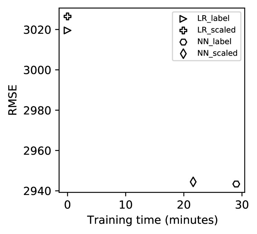
(a) MongoDB

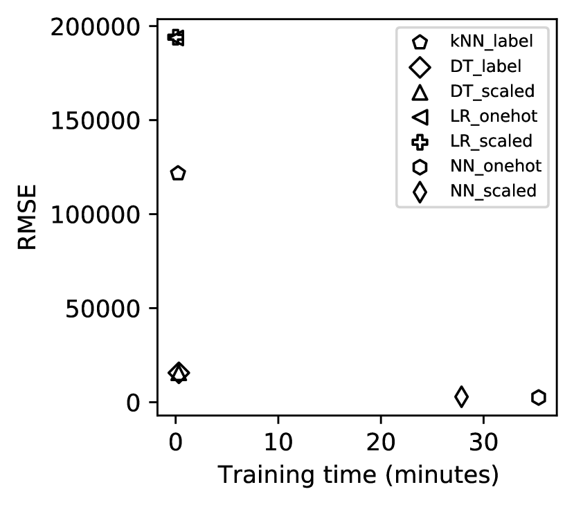
(b) Lrzip

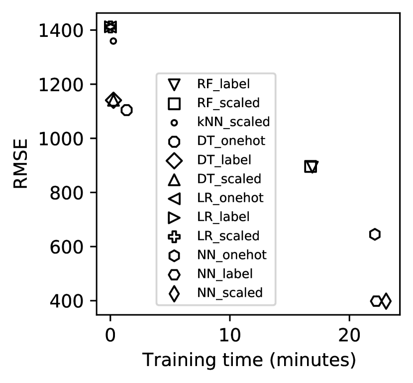
(c) Trimesh

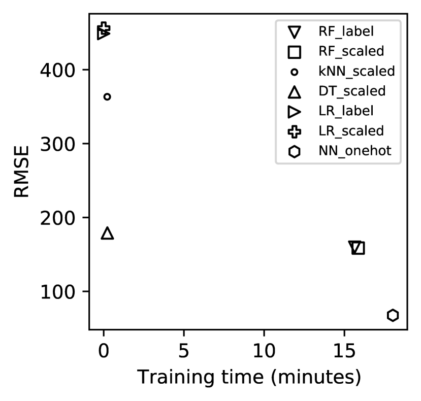
(d) ExaStencils

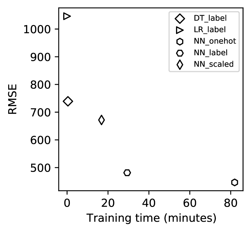
(e) x264

Figure 3. The trade-off between RMSE and training time over all Pareto-optimal model-encoding pairs.

4.2.1. Method

To study RQ2, we compare all RMSE values for the three encoding schemes under the models and systems. That is, for each subject system, there are $3\times 7=21$ pairs of model-encoding (50 RMSE repeats each). To ensure statistical significance among the comparisons, we use Scott-Knott test to assign a score for each pair, hence similar ones are clustered together (same score) while different ones can be ranked (the higher score, the better).

4.2.2. Results

As illustrated in Table 3, we observe some interesting findings:

• Finding 3: From Table 3f, overall, label and one-hot encoding are clearly more accurate than scaled label encoding across the models, as the former two have the best total Scott-Knott scores for all models over the systems studied. Between these two, one-hot encoding tends to be slightly better across all models, as it wins on 4 models against the 3 wins by label encoding. We observe similar trend from Table 3a to 3e over the systems.

• Finding 4: For different models in Table 3f, we observe that one-hot encoding is the best for deep learning, lazy, and kernel models while label encoding is preferred on linear and tree models. The same has also been registered in Table 3a to 3e.

• Finding 5: From Table 3a to 3e, NN is clearly amongst the top models on Scott-Knott score and RMSE regardless of the encoding schemes and systems. In particular, when NN is chosen, NN_onehot is the best, as it has a better Scott-Knott score than the other two on 3 out of 5 systems, draw on one system and lose on the remaining one, leading to a 75% cases of no worse outcome than NN_label and NN_scaled.

To conclude, we can answer RQ2 as:

4.3. RQ3: Training Time

4.3.1. Research

Similar to RQ2, here we measured the training time over 50 runs for all 21 pairs of model-encoding for each system.

4.3.2. Results

With Table 4, we can observe some patterns:

• Finding 6: Overall, from Table 4f, label and scaled label encoding are much faster to train than their one-hot counterpart, which has never won the other two under any model across the systems. In particular, scaled label encoding appears to have the fastest training than others in general, as the former wins on 4 models, draws on one, and loses only on two. Similar results have been obtained in Table 4a to 4e.

• Finding 7: For different model types, in Table 4f, the label encoding tends to be the best option in terms of training time for tree model and lazy model; the scaled label counterpart is faster on deep learning model, linear model, and kernel model. This is similar to that from Table 4a to 4e.

• Finding 8: From Table 4a to 4e, unexpectedly LR has the fastest training time over all systems and this model works the best with scaled label encoding since LR_scaled is the fastest on 4 out of 5 systems; its difference to LR_label tends to be marginal though.

Therefore, we say:

4.4. RQ4: Trade-off Analysis

4.4.1. Method

Understanding RQ4 requires us to simultaneously consider the accuracy and training time achieved by all 21 pairs of model-encoding. According to the guidance provided by Li and Chen (Li et al., ress), for each system, we seek to analyze the Pareto optimal choices as those are the ones that require trade-offs. Suppose that a pair $P_{x}$ has $\{A_{x},T_{x}\}$ and another $P_{y}$ comes with $\{A_{y},T_{y}\}$, whereby $A_{x}$ and $A_{y}$ are their median RMSE (over 50 runs) while $T_{x}$ and $T_{y}$ are their median training time, respectively. We say $P_{x}$ dominates $P_{y}$ if $A_{x}\leq A_{y}$ and $T_{x}\leq T_{y}$ while there is either $A_{x}<A_{y}$ or $T_{x}<T_{y}$. A pair, which is not dominated by any other pairs from the total set of 21, is called a Pareto-optimal pair therein. The set of all Pareto-optimal points is called the Pareto front (Figures 3). We also plot the Pareto front with respect to the total Scott-Knott scores (over all systems) under each model (Figures 4).

Here, a Pareto-optimal pair that has the best accuracy or the fastest training time is called a biased point (or an extreme point). Among others, we are interested in the non-extreme, less biased points, especially those with a well-balanced trade-off.

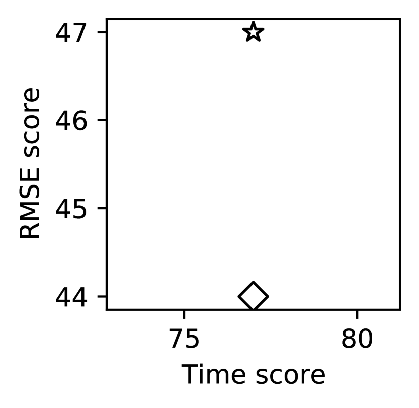
(a) DT

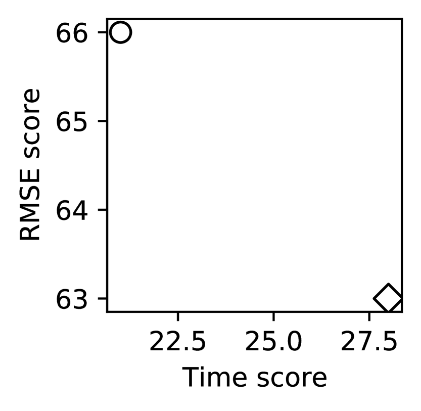
(b) NN

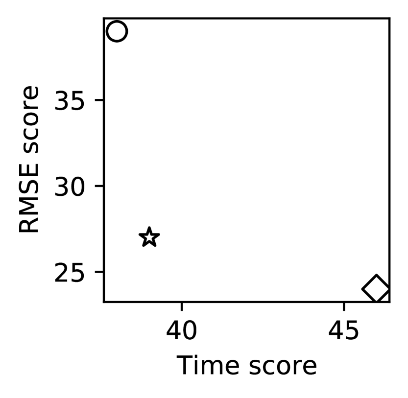
(c) KRR

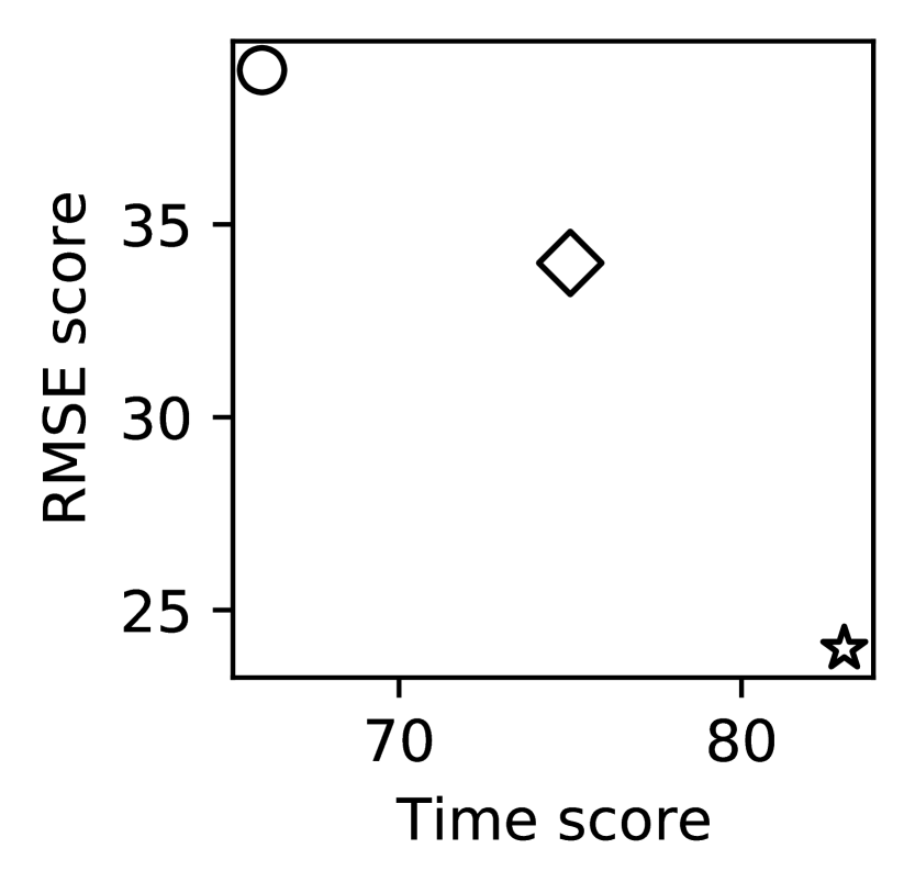
(d) $k$NN

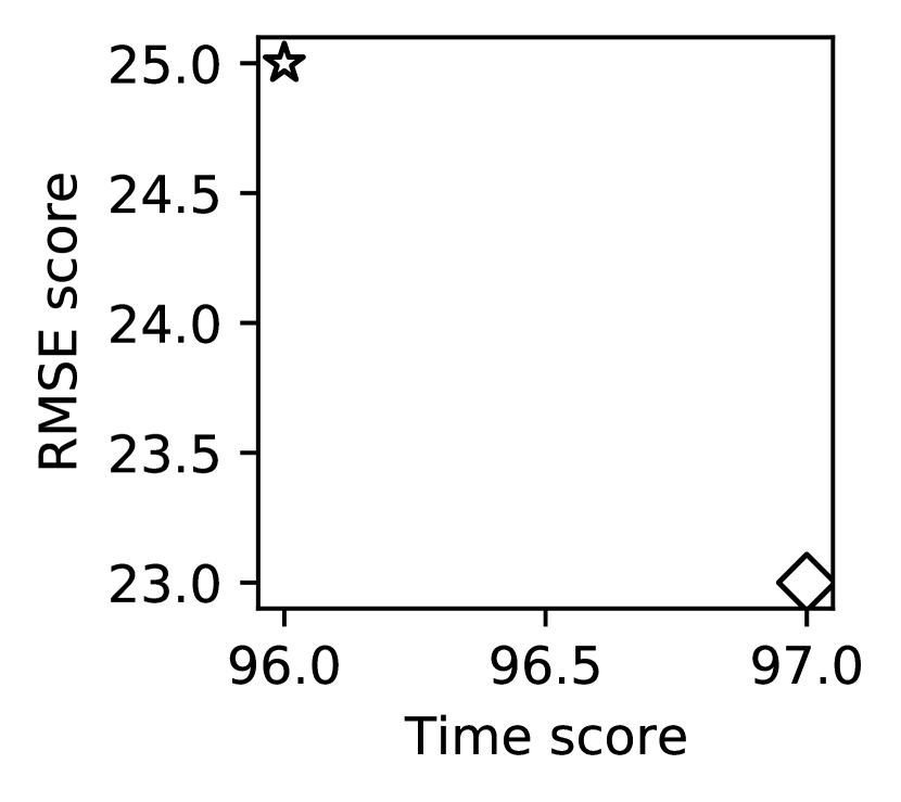
(e) LR

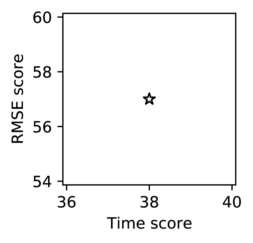
(f) RF

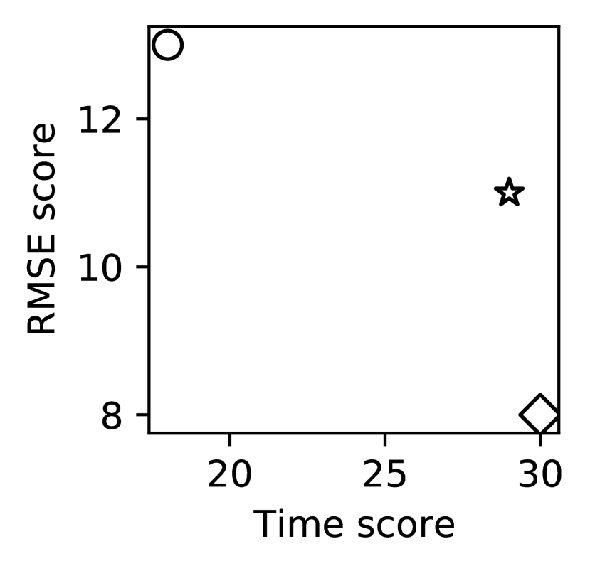
(g) SVR

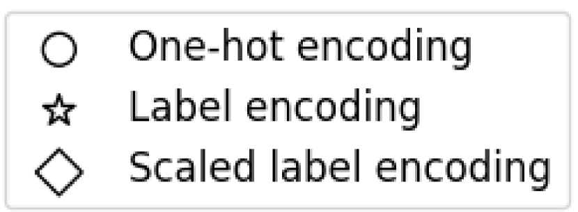
Figure 4. The total Scott-Knott scores for each model over all systems. Only the Pareto-optimal choice are presented.

4.4.2. Results

The results are illustrated in Figures 3 and 4, from which we obtain some interesting observations:

• Finding 9: Over all the model-encoding pairs (Figures 3), label and scaled label encoding can more commonly lead to less biased results (non-extreme points) in the Pareto front than their one-hot counterpart. This can clearly offer more trade-off choices.

• Finding 10: In Figures 3, the scaled label encoding tends to achieve more balanced trade-off than the others, but the paired model may vary, i.e., it can be NN, DT, or RF, across the systems. For example, it is NN_scaled on MongoDB but becomes DT_scaled on Lrzip.

• Finding 11: Kernel models like KRR and SVR have never produced Pareto-optimal outcomes over the 5 systems studied (Figures 3).

• Finding 12: From Figure 4, only kernel and lazy models have relatively less biased point in their own Pareto front, which are achieved by label (Figure 4c and 4g) and scaled label encoding (Figure 4d), respectively.

In summary, we have:

5. Actionable Suggestions

In this section, we discuss the suggestions on the encoding scheme for learning software performance under a variety of circumstances.

From RQ1, it can be rather time-consuming for comparing all three encoding schemes under RF, SVR, KRR or NN. Indeed, the “efforts” may be reduced if we consider, e.g., less repeated runs or even reduced data samples. However, to provide a reliable choice, what we consider in this study is essential, and hence further reducing them may increase the instability of the result. The process can be even more expensive if different models are also to be assessed during the trial-and-error. In contrast, when $k$NN, DT, or LR is to be used, it only requires less than one hour each — an assumption that may be more acceptable within the development lifecycle.

Reflecting on RQ2, when only the accuracy is of concern, we can make suggestions for practitioners to infer the best choice of encoding schemes when experimental assessment is not possible or desirable. Among others, it is clear that NN tends to offer the best accuracy, and NN paired with one-hot encoding, i.e., NN_onehot, is the most reliable choice. In contrast, scaled label encoding often performs the worst, and hence scaled label encoding can be ruled out from the suggestions.

Besides the fact that the one-hot encoding can generally lead to the best accuracy over the models, we do observe some specific patterns when the model to be used is fixed: one-hot encoding for deep learning and kernel models while label encoding for linear and tree models.

Deriving from the findings for RQ3, if the training time is of higher importance, we can also estimate the suitable choice of encoding scheme in the absence of experimental evaluation. Over all possible models studied, linear regression is unexpectedly the fastest to train and when it is paired with scaled label encoding (LR_scaled) the training is the fastest. One-hot encoding is often the slowest to train, and hence can be avoided.

Although the scaled label encoding appears to be faster to train than its label counterpart, they remain competitive. In fact, when the model to be used has been pre-defined, we observe some common patterns: the scaled label encoding is the best for deep learning, linear, and kernel models while the label encoding is preferred for tree and lazy models.

It is not uncommon that the preference between accuracy and training time can be unclear, and hence an unbiased outcome is important. According to the findings for RQ4, this needs the label and scaled label encoding. Because in this case, as we have shown, they often lead to results that are in the middle of the Pareto front for the pairs. In particular, scaled label encoding can often lead to well-balanced results in contrast to the other, but the paired model may vary. We would also suggest avoiding one-hot encoding and kernel model (SVR and KRR), as the former would easily bias to accuracy or training time while the latter leads to no Pareto optimal choice at all over the systems studied.

However, when the model needs to be fixed, only the kernel and lazy models can have less biased choices, which are under the label and scaled label encoding, respectively.

6. Discussion

We now discuss a few interesting points derived from our study.

6.1. Practicality of Performance Models

The performance models built can be used in different practical scenarios, under each of which the accuracy and training time can be of great importance (and thereby the choice of encoding schemes are equally crucial).

6.1.1. Configuration debugging

Ill-fitted Configurations can lead to bugs such that the resulted performance is dramatically worse than the expectation. Here, a performance model can help software engineers easily inspect which configuration options are likely to be the root cause of the bug and identify the potential fix (Xu et al., 2015). The fact that the model makes inferences without running the system can greatly improve the efficiency of the debugging process. Further, by analyzing the models, software engineers can gain a better understanding of the system’s performance characteristics which helps to prevent future configuration bugs.

6.1.2. Speed up automatic configuration tuning

Automatic configuration tuning is necessary to optimize the performance of the software system at deployment time. However, due to the expensiveness of measuring the performance, tuning is often a slow and time-consuming process. As one resolution to that issue, the performance model can serve as the surrogate for cheap evaluation of the configuration. Indeed, there have been a few successful applications in this regard, such as those that rely on Bayesian optimization (Nair et al., 2020; Jamshidi and Casale, 2016).

6.1.3. Runtime self-adaptation

Self-adapting the configuration at runtime is a promising way to manage the system’s performance under uncertain environments. In this context, the performance model can help to achieve the adaptation in a timely manner, as it offers a relatively cheap way to reason about the better or worse of different configurations under changing environmental conditions. From the literature of self-adaptive systems, it is not uncommon to see that the performance models are often used during the planning stage (Chen and Bahsoon, 2017b; Chen et al., 2018b, a, 2020; Chen, 2022; Chen and Bahsoon, 2014).

6.2. Why Considering Different Models?

We note that some learning models perform overwhelmingly better than the others, such as NN. Yet, our study involves a diverse set of models because, in practice, there may be other reasons that a learning model is preferred. For example, linear and tree models may be used as they are directly interpretable (Siegmund et al., 2012; Valov et al., 2015), despite that they can lead to inferior accuracy overall. Therefore, our results on the choice of encoding schemes provide evidence for a wide set of scenarios and the possibility that different models may be involved.

The other reason for considering different models is that we seek to examine whether the choice of machine learning model matters when deicing what encoding schemes to use. Indeed, our results show that the paired model is an integral part and we provide detailed suggestions in that regard.

6.3. On Interactions between Configuration Options

The encoding schemes can serve as different ways to represent the interactions between configuration options. Since the one-hot encoding embeds the values of options as the feature dimensions and captures their interactions, it models a much more finer-grained feature space compared with that of the label and scaled-label counterparts. Our results show that, indeed, such a finer-grained capture of interactions enables one-hot encoding to become the most reliable scheme across the models/software as it has the generally best accuracy. This confirms the current understanding that the interaction between configuration options is important and the way how they are handled can significantly influence the accuracy (Siegmund et al., 2012). Most importantly, our findings show that it is possible to better handle the interactions at the level of encoding.

7. Threats to validity

Similar to many empirical studies in software engineering, our work is subject to threats to validity. Specifically, internal threats can be related to the configuration options used and their ranges. Indeed, a different set may lead to a different result in some cases. However, here we follow what has been commonly used in state-of-the-art studies, which are representatives for the subject systems. The hyperparameter of the models to tune can also impose this threat. Ideally, widening the set of hyperparameters to tune can complement our results. Yet, considering an extensive set of hyperparameters is rather expensive, as the tuning needs to go through the full training and validation process. To mitigate such, we have examined different hyperparameters in preliminary runs for finding a balance between effectiveness and overhead.

Construct threats to validity can be related to the metric used. While different metrics exist for measuring accuracy, here we use RMSE, which is a widely used one for learning software performance. The results are also evaluated validated Scott-Knott test (Mittas and Angelis, 2013). We also set a data samples of $5,000$, which tends to be reasonable as this is what has been commonly used in prior work (Dorn et al., 2020; Johnsson et al., 2019; Shao et al., 2019; Gerostathopoulos et al., 2018). Indeed, using other metrics or different sample size may offer new insights, which we plan to do in future work.

Finally, external threats to validity can raise from the subjects and models used. To mitigate such, we study five commonly studied systems that are of diverse characteristics, together with seven widely-used models. This leads to a total of 105 cases of investigation. Such a setting, although not exhaustive, is not uncommon in empirical software engineering and can serve as a strong foundation to generalize our findings, especially considering that an exhaustive study of all possible models and systems is unrealistic. Yet, we agree that additional subjects may prove fruitful.

8. Related Work

A most widely used representation for building machine learning-based software performance model is the one-hot encoding (Siegmund et al., 2012; Guo et al., 2013; Bao et al., 2019). The root motivation of such encoding is derived from the fact that a configurable system can be represented by the feature model — a tree-liked structure that captures the variability (Siegmund et al., 2012). In a feature model, each feature can be selected or deselected, which is naturally a binary option. Note that categorical and numeric configuration options can also be captured in the feature model, as long as they can be discretized (Chen et al., 2018c). Following this, several approaches have been developed using machine learning. Among others, Guo et al. (Guo et al., 2013) use the one-hot encoding combined with the DT to predict software performance, as it fits well with the feature model. Bao et al. (Bao et al., 2019) also use the same encoding, and their claim is that it can better capture the options which have no ordinal relationships.

The other, perhaps more natural, encoding scheme for learning software performance is the label encoding, which has also been followed by many studies, either with (Chen, 2019; Chen and Bahsoon, 2017a; Ha and Zhang, 2019) or without scaling (Nair et al., 2020; Siegmund et al., 2015; Nair et al., 2017). For example, Chen and Bahsoon (Chen and Bahsoon, 2017a) directly encode the configuration options to learn the performance model with normalization to $[0,1]$. Siegmund et al. (Siegmund et al., 2015) also follows the label encoding, but the binary and numeric configuration options are treated differently in the model learned with no normalization.

However, the choice between those two encoding schemes for software performance learning often lacks systematic justification, which is the gap that this empirical study aims to bridge.

In the other domains, the importance of choosing the encoding schemes for building machine learning models has been discussed. For example, Jackson and Agrawal (Jackson and Agrawal, 2019) compare the most common encoding schemes for predicting security events using logs. The result shows that it is considerably harmful to encode the representation without systematic justification. Similarly, He and Parida (He and Parida, 2016) study the effect of two encoding schemes for genetic trait prediction. A thorough analysis of the encoding schemes has been provided, together with which could be better under what cases. However, those findings cannot be directly applied in the context of software performance learning, due to two of its properties:

• Sampling from the configurable systems is rather expensive (Zuluaga et al., 2013; Nair et al., 2020; Jamshidi and Casale, 2016), thus the sample size is often relatively smaller.

• Software configuration is often sparse, i.e., the close configurations may have rather different performance (Nair et al., 2020; Jamshidi and Casale, 2016). This is because options like cache, when enabled, can create significant implications to the performance, but such a change is merely represented as a one-bit difference in the model. Therefore, the distribution of the data samples can be intrinsically different from the other domains.

Most importantly, this work provides an in-depth understanding of this topic for learning software performance, together with insights and suggestions under different circumstances.

9. Conclusions

This paper bridges a gap in the understating of encoding schemes for learning performance for highly configurable software. We do that by conducting a systematic empirical study, covering five systems, seven models, and three widely used encoding schemes, giving a total of 105 cases of investigation. In summary, we show that

Choosing the encoding scheme is non-trivial for performance learning and it can be rather expensive to do it using trial-and-error in a case-by-case manner.

Our findings provide actionable suggestions and “rule-of-thumb” when a thorough experimental comparison is not possible or desirable. Among these, the most important ones over all models and encoding schemes are:

• using neural network paired with one-hot encoding for the best accuracy.

• using linear regression paired with scaled label encoding for the fastest training.

• using scaled label encoding for a relatively well-balanced outcome, but mind the underlying model.

We hope that this work can serve as a good starting point to raise the awareness of the importance of choosing encoding schemes for performance learning, and the actionable suggestions are of usefulness to the practitioners in the field. More importantly, we seek to spark a dialog on a set of relevant future research directions for this regard. As such, the next stage on this research thread is vast, including designing specialized models paired with suitable encoding schemes or even investigating new, tailored encoding schemes derived from the findings in the paper.

References

- (1)
- Alaya et al. (2019) Mokhtar Z. Alaya, Simon Bussy, Stéphane Gaïffas, and Agathe Guilloux. 2019. Binarsity: a penalization for one-hot encoded features in linear supervised learning. J. Mach. Learn. Res. 20 (2019), 118:1–118:34. http://jmlr.org/papers/v20/17-170.html
- Bao et al. (2019) Liang Bao, Xin Liu, Fangzheng Wang, and Baoyin Fang. 2019. ACTGAN: Automatic Configuration Tuning for Software Systems with Generative Adversarial Networks. In 34th IEEE/ACM International Conference on Automated Software Engineering, ASE 2019, San Diego, CA, USA, November 11-15, 2019. IEEE, 465–476. https://doi.org/10.1109/ASE.2019.00051
- Chai and Draxler (2014) Tianfeng Chai and Roland R Draxler. 2014. Root mean square error (RMSE) or mean absolute error (MAE)?–Arguments against avoiding RMSE in the literature. Geoscientific model development 7, 3 (2014), 1247–1250.
- Chen (2019) Tao Chen. 2019. All versus one: an empirical comparison on retrained and incremental machine learning for modeling performance of adaptable software. In Proceedings of the 14th International Symposium on Software Engineering for Adaptive and Self-Managing Systems, SEAMS@ICSE 2019, Montreal, QC, Canada, May 25-31, 2019, Marin Litoiu, Siobhán Clarke, and Kenji Tei (Eds.). ACM, 157–168. https://doi.org/10.1109/SEAMS.2019.00029
- Chen (2022) Tao Chen. 2022. Lifelong dynamic optimization for self-adaptive systems: fact or fiction?. In SANER ’22: 29th IEEE International Conference on Software Analysis, Evolution and Reengineering, Hawaii, United States, March 15-18 2022. IEEE.
- Chen and Bahsoon (2013) Tao Chen and Rami Bahsoon. 2013. Self-adaptive and sensitivity-aware QoS modeling for the cloud. In Proceedings of the 8th International Symposium on Software Engineering for Adaptive and Self-Managing Systems, SEAMS 2013, San Francisco, CA, USA, May 20-21, 2013, Marin Litoiu and John Mylopoulos (Eds.). IEEE Computer Society, 43–52. https://doi.org/10.1109/SEAMS.2013.6595491
- Chen and Bahsoon (2014) Tao Chen and Rami Bahsoon. 2014. Symbiotic and sensitivity-aware architecture for globally-optimal benefit in self-adaptive cloud. In 9th International Symposium on Software Engineering for Adaptive and Self-Managing Systems, SEAMS 2014, Proceedings, Hyderabad, India, June 2-3, 2014, Gregor Engels and Nelly Bencomo (Eds.). ACM, 85–94. https://doi.org/10.1145/2593929.2593931
- Chen and Bahsoon (2017a) Tao Chen and Rami Bahsoon. 2017a. Self-Adaptive and Online QoS Modeling for Cloud-Based Software Services. IEEE Trans. Software Eng. 43, 5 (2017), 453–475. https://doi.org/10.1109/TSE.2016.2608826
- Chen and Bahsoon (2017b) Tao Chen and Rami Bahsoon. 2017b. Self-Adaptive Trade-off Decision Making for Autoscaling Cloud-Based Services. IEEE Trans. Serv. Comput. 10, 4 (2017), 618–632. https://doi.org/10.1109/TSC.2015.2499770
- Chen et al. (2018b) Tao Chen, Rami Bahsoon, Shuo Wang, and Xin Yao. 2018b. To Adapt or Not to Adapt?: Technical Debt and Learning Driven Self-Adaptation for Managing Runtime Performance. In Proceedings of the 2018 ACM/SPEC International Conference on Performance Engineering, ICPE 2018, Berlin, Germany, April 09-13, 2018, Katinka Wolter, William J. Knottenbelt, André van Hoorn, and Manoj Nambiar (Eds.). ACM, 48–55. https://doi.org/10.1145/3184407.3184413
- Chen et al. (2014) Tao Chen, Rami Bahsoon, and Xin Yao. 2014. Online QoS Modeling in the Cloud: A Hybrid and Adaptive Multi-learners Approach. In Proceedings of the 7th IEEE/ACM International Conference on Utility and Cloud Computing, UCC 2014, London, United Kingdom, December 8-11, 2014. IEEE Computer Society, 327–336. https://doi.org/10.1109/UCC.2014.42
- Chen et al. (2018a) Tao Chen, Rami Bahsoon, and Xin Yao. 2018a. A Survey and Taxonomy of Self-Aware and Self-Adaptive Cloud Autoscaling Systems. ACM Comput. Surv. 51, 3 (2018), 61:1–61:40. https://doi.org/10.1145/3190507
- Chen et al. (2020) Tao Chen, Rami Bahsoon, and Xin Yao. 2020. Synergizing Domain Expertise With Self-Awareness in Software Systems: A Patternized Architecture Guideline. Proc. IEEE 108, 7 (2020), 1094–1126. https://doi.org/10.1109/JPROC.2020.2985293
- Chen et al. (2018c) Tao Chen, Ke Li, Rami Bahsoon, and Xin Yao. 2018c. FEMOSAA: Feature-Guided and Knee-Driven Multi-Objective Optimization for Self-Adaptive Software. ACM Trans. Softw. Eng. Methodol. 27, 2 (2018), 5:1–5:50. https://doi.org/10.1145/3204459
- Chen and Li (2021a) Tao Chen and Miqing Li. 2021a. MMO: Meta Multi-Objectivization for Software Configuration Tuning. CoRR abs/2112.07303 (2021). arXiv:2112.07303 https://arxiv.org/abs/2112.07303
- Chen and Li (2021b) Tao Chen and Miqing Li. 2021b. Multi-objectivizing software configuration tuning. In ESEC/FSE ’21: 29th ACM Joint European Software Engineering Conference and Symposium on the Foundations of Software Engineering, Athens, Greece, August 23-28, 2021, Diomidis Spinellis, Georgios Gousios, Marsha Chechik, and Massimiliano Di Penta (Eds.). ACM, 453–465. https://doi.org/10.1145/3468264.3468555
- Cortes and Vapnik (1995) Corinna Cortes and Vladimir Vapnik. 1995. Support-vector networks. Machine learning 20, 3 (1995), 273–297.
- Didona et al. (2015) Diego Didona, Francesco Quaglia, Paolo Romano, and Ennio Torre. 2015. Enhancing Performance Prediction Robustness by Combining Analytical Modeling and Machine Learning. In Proceedings of the 6th ACM/SPEC International Conference on Performance Engineering, Austin, TX, USA, January 31 - February 4, 2015, Lizy K. John, Connie U. Smith, Kai Sachs, and Catalina M. Lladó (Eds.). ACM, 145–156. https://doi.org/10.1145/2668930.2688047
- Dorn et al. (2020) Johannes Dorn, Sven Apel, and Norbert Siegmund. 2020. Mastering Uncertainty in Performance Estimations of Configurable Software Systems. In 35th IEEE/ACM International Conference on Automated Software Engineering, ASE 2020, Melbourne, Australia, September 21-25, 2020. IEEE, 684–696. https://doi.org/10.1145/3324884.3416620
- Fei et al. (2016) Jingzhou Fei, Ningbo Zhao, Yong Shi, Yongming Feng, and Zhongwei Wang. 2016. Compressor performance prediction using a novel feed-forward neural network based on Gaussian kernel function. Advances in Mechanical Engineering 8, 1 (2016), 1687814016628396.
- Fix (1985) Evelyn Fix. 1985. Discriminatory analysis: nonparametric discrimination, consistency properties. Vol. 1. USAF school of Aviation Medicine.
- Gerostathopoulos et al. (2018) Ilias Gerostathopoulos, Christian Prehofer, and Tomás Bures. 2018. Adapting a system with noisy outputs with statistical guarantees. In Proceedings of the 13th International Conference on Software Engineering for Adaptive and Self-Managing Systems, SEAMS@ICSE 2018, Gothenburg, Sweden, May 28-29, 2018, Jesper Andersson and Danny Weyns (Eds.). ACM, 58–68. https://doi.org/10.1145/3194133.3194152
- Goldin (2010) Rebecca F. Goldin. 2010. Review: Statistical Models: Theory and Practice (Revised Edition). Cambridge University Press, New York, New York, 2009, xiv + 442 pp., ISBN 978-0-521-74385-3, $40. by David A. Freedman. Am. Math. Mon. 117, 9 (2010), 844–847. https://doi.org/10.4169/000298910X521733
- Grohmann et al. (2020) Johannes Grohmann, Daniel Seybold, Simon Eismann, Mark Leznik, Samuel Kounev, and Jörg Domaschka. 2020. Baloo: Measuring and Modeling the Performance Configurations of Distributed DBMS. In 28th International Symposium on Modeling, Analysis, and Simulation of Computer and Telecommunication Systems, MASCOTS 2020, Nice, France, November 17-19, 2020. IEEE, 1–8. https://doi.org/10.1109/MASCOTS50786.2020.9285960
- Guo et al. (2013) Jianmei Guo, Krzysztof Czarnecki, Sven Apel, Norbert Siegmund, and Andrzej Wasowski. 2013. Variability-aware performance prediction: A statistical learning approach. In 2013 28th IEEE/ACM International Conference on Automated Software Engineering, ASE 2013, Silicon Valley, CA, USA, November 11-15, 2013, Ewen Denney, Tevfik Bultan, and Andreas Zeller (Eds.). IEEE, 301–311. https://doi.org/10.1109/ASE.2013.6693089
- Ha and Zhang (2019) Huong Ha and Hongyu Zhang. 2019. DeepPerf: performance prediction for configurable software with deep sparse neural network. In Proceedings of the 41st International Conference on Software Engineering, ICSE 2019, Montreal, QC, Canada, May 25-31, 2019, Joanne M. Atlee, Tevfik Bultan, and Jon Whittle (Eds.). IEEE / ACM, 1095–1106. https://doi.org/10.1109/ICSE.2019.00113
- Han and Yu (2016) Xue Han and Tingting Yu. 2016. An Empirical Study on Performance Bugs for Highly Configurable Software Systems. In Proceedings of the 10th ACM/IEEE International Symposium on Empirical Software Engineering and Measurement, ESEM 2016, Ciudad Real, Spain, September 8-9, 2016. ACM, 23:1–23:10. https://doi.org/10.1145/2961111.2962602
- He and Parida (2016) Dan He and Laxmi Parida. 2016. Does encoding matter? A novel view on the quantitative genetic trait prediction problem. BMC Bioinform. 17, S-9 (2016), 272. https://doi.org/10.1186/s12859-016-1127-1
- Hinton (2012) Geoffrey E. Hinton. 2012. A Practical Guide to Training Restricted Boltzmann Machines. In Neural Networks: Tricks of the Trade - Second Edition, Grégoire Montavon, Genevieve B. Orr, and Klaus-Robert Müller (Eds.). Lecture Notes in Computer Science, Vol. 7700. Springer, 599–619. https://doi.org/10.1007/978-3-642-35289-8_32
- Ho (1995) Tin Kam Ho. 1995. Random decision forests. In Third International Conference on Document Analysis and Recognition, ICDAR 1995, August 14 - 15, 1995, Montreal, Canada. Volume I. IEEE Computer Society, 278–282. https://doi.org/10.1109/ICDAR.1995.598994
- Iorio et al. (2019) Francesco Iorio, Ali B. Hashemi, Michael Tao, and Cristiana Amza. 2019. Transfer Learning for Cross-Model Regression in Performance Modeling for the Cloud. In 2019 IEEE International Conference on Cloud Computing Technology and Science (CloudCom), Sydney, Australia, December 11-13, 2019. IEEE, 9–18. https://doi.org/10.1109/CloudCom.2019.00015
- Jackson and Agrawal (2019) Eric Jackson and Rajeev Agrawal. 2019. Performance Evaluation of Different Feature Encoding Schemes on Cybersecurity Logs. In 2019 SoutheastCon. 1–9. https://doi.org/10.1109/SoutheastCon42311.2019.9020560
- Jamshidi and Casale (2016) Pooyan Jamshidi and Giuliano Casale. 2016. An Uncertainty-Aware Approach to Optimal Configuration of Stream Processing Systems. In 24th IEEE International Symposium on Modeling, Analysis and Simulation of Computer and Telecommunication Systems, MASCOTS 2016, London, United Kingdom, September 19-21, 2016. IEEE Computer Society, 39–48. https://doi.org/10.1109/MASCOTS.2016.17
- Johnsson et al. (2019) Andreas Johnsson, Farnaz Moradi, and Rolf Stadler. 2019. Performance Prediction in Dynamic Clouds using Transfer Learning. In IFIP/IEEE International Symposium on Integrated Network Management, IM 2019, Washington, DC, USA, April 09-11, 2019, Joe Betser, Carol J. Fung, Alex Clemm, Jérôme François, and Shingo Ata (Eds.). IFIP, 242–250. http://dl.ifip.org/db/conf/im/im2019/189279.pdf
- Kaltenecker et al. (2020) Christian Kaltenecker, Alexander Grebhahn, Norbert Siegmund, and Sven Apel. 2020. The Interplay of Sampling and Machine Learning for Software Performance Prediction. IEEE Softw. 37, 4 (2020), 58–66. https://doi.org/10.1109/MS.2020.2987024
- Li et al. (2020) Ke Li, Zilin Xiang, Tao Chen, Shuo Wang, and Kay Chen Tan. 2020. Understanding the automated parameter optimization on transfer learning for cross-project defect prediction: an empirical study. In ICSE ’20: 42nd International Conference on Software Engineering, Seoul, South Korea, 27 June - 19 July, 2020, Gregg Rothermel and Doo-Hwan Bae (Eds.). ACM, 566–577. https://doi.org/10.1145/3377811.3380360
- Li et al. (ress) Miqing Li, Tao Chen, and Xin Yao. 2020, in press. How to Evaluate Solutions in Pareto-based Search-Based Software Engineering? A Critical Review and Methodological Guidance. IEEE Transactions on Software Engineering (2020, in press). https://doi.org/10.1109/TSE.2020.3036108
- Mittas and Angelis (2013) Nikolaos Mittas and Lefteris Angelis. 2013. Ranking and Clustering Software Cost Estimation Models through a Multiple Comparisons Algorithm. IEEE Trans. Software Eng. 39, 4 (2013), 537–551. https://doi.org/10.1109/TSE.2012.45
- Mohr et al. (2021) Felix Mohr, Marcel Wever, Alexander Tornede, and Eyke Hullermeier. 2021. Predicting Machine Learning Pipeline Runtimes in the Context of Automated Machine Learning. IEEE Transactions on Pattern Analysis and Machine Intelligence (2021).
- Nair et al. (2017) Vivek Nair, Tim Menzies, Norbert Siegmund, and Sven Apel. 2017. Using bad learners to find good configurations. In Proceedings of the 2017 11th Joint Meeting on Foundations of Software Engineering, ESEC/FSE 2017, Paderborn, Germany, September 4-8, 2017, Eric Bodden, Wilhelm Schäfer, Arie van Deursen, and Andrea Zisman (Eds.). ACM, 257–267. https://doi.org/10.1145/3106237.3106238
- Nair et al. (2020) Vivek Nair, Zhe Yu, Tim Menzies, Norbert Siegmund, and Sven Apel. 2020. Finding Faster Configurations Using FLASH. IEEE Trans. Software Eng. 46, 7 (2020), 794–811. https://doi.org/10.1109/TSE.2018.2870895
- Pan et al. (2016) Jiaqi Pan, Yan Zhuang, and Simon Fong. 2016. The impact of data normalization on stock market prediction: using SVM and technical indicators. In International Conference on Soft Computing in Data Science. Springer, 72–88.
- Pedregosa et al. (2011) Fabian Pedregosa, Gaël Varoquaux, Alexandre Gramfort, Vincent Michel, Bertrand Thirion, Olivier Grisel, Mathieu Blondel, Peter Prettenhofer, Ron Weiss, Vincent Dubourg, Jake VanderPlas, Alexandre Passos, David Cournapeau, Matthieu Brucher, Matthieu Perrot, and Edouard Duchesnay. 2011. Scikit-learn: Machine Learning in Python. J. Mach. Learn. Res. 12 (2011), 2825–2830. http://dl.acm.org/citation.cfm?id=2078195
- Peng et al. (2021) Kewen Peng, Christian Kaltenecker, Norbert Siegmund, Sven Apel, and Tim Menzies. 2021. VEER: Disagreement-Free Multi-objective Configuration. CoRR abs/2106.02716 (2021). arXiv:2106.02716 https://arxiv.org/abs/2106.02716
- Queiroz et al. (2016) Rodrigo Queiroz, Thorsten Berger, and Krzysztof Czarnecki. 2016. Towards predicting feature defects in software product lines. In Proceedings of the 7th International Workshop on Feature-Oriented Software Development, FOSD@SPLASH 2016, Amsterdam, Netherlands, October 30, 2016, Christoph Seidl and Leopoldo Teixeira (Eds.). ACM, 58–62. https://doi.org/10.1145/3001867.3001874
- Rokach and Maimon (2014) Lior Rokach and Oded Maimon. 2014. Data Mining with Decision Trees - Theory and Applications. 2 Edition. Series in Machine Perception and Artificial Intelligence, Vol. 81. WorldScientific. https://doi.org/10.1142/9097
- Shao et al. (2019) Jingyu Shao, Qing Wang, and Fangbing Liu. 2019. Learning to Sample: An Active Learning Framework. In 2019 IEEE International Conference on Data Mining, ICDM 2019, Beijing, China, November 8-11, 2019, Jianyong Wang, Kyuseok Shim, and Xindong Wu (Eds.). IEEE, 538–547. https://doi.org/10.1109/ICDM.2019.00064
- Siegmund et al. (2015) Norbert Siegmund, Alexander Grebhahn, Sven Apel, and Christian Kästner. 2015. Performance-influence models for highly configurable systems. In Proceedings of the 2015 10th Joint Meeting on Foundations of Software Engineering, ESEC/FSE 2015, Bergamo, Italy, August 30 - September 4, 2015, Elisabetta Di Nitto, Mark Harman, and Patrick Heymans (Eds.). ACM, 284–294. https://doi.org/10.1145/2786805.2786845
- Siegmund et al. (2012) Norbert Siegmund, Sergiy S. Kolesnikov, Christian Kästner, Sven Apel, Don S. Batory, Marko Rosenmüller, and Gunter Saake. 2012. Predicting performance via automated feature-interaction detection. In 34th International Conference on Software Engineering, ICSE 2012, June 2-9, 2012, Zurich, Switzerland, Martin Glinz, Gail C. Murphy, and Mauro Pezzè (Eds.). IEEE Computer Society, 167–177. https://doi.org/10.1109/ICSE.2012.6227196
- Valov et al. (2015) Pavel Valov, Jianmei Guo, and Krzysztof Czarnecki. 2015. Empirical comparison of regression methods for variability-aware performance prediction. In Proceedings of the 19th International Conference on Software Product Line, SPLC 2015, Nashville, TN, USA, July 20-24, 2015, Douglas C. Schmidt (Ed.). ACM, 186–190. https://doi.org/10.1145/2791060.2791069
- Vargha and Delaney (2000) András Vargha and Harold D. Delaney. 2000. A Critique and Improvement of the CL Common Language Effect Size Statistics of McGraw and Wong.
- Vovk (2013) Vladimir Vovk. 2013. Kernel ridge regression. In Empirical inference. Springer, 105–116.
- Wang (2003) Sun-Chong Wang. 2003. Artificial neural network. In Interdisciplinary computing in java programming. Springer, 81–100.
- Xia et al. (2018) Tianpei Xia, Rahul Krishna, Jianfeng Chen, George Mathew, Xipeng Shen, and Tim Menzies. 2018. Hyperparameter Optimization for Effort Estimation. CoRR abs/1805.00336 (2018). arXiv:1805.00336 http://arxiv.org/abs/1805.00336
- Xu et al. (2015) Tianyin Xu, Long Jin, Xuepeng Fan, Yuanyuan Zhou, Shankar Pasupathy, and Rukma Talwadker. 2015. Hey, you have given me too many knobs!: understanding and dealing with over-designed configuration in system software. In Proceedings of the 2015 10th Joint Meeting on Foundations of Software Engineering, ESEC/FSE 2015, Bergamo, Italy, August 30 - September 4, 2015, Elisabetta Di Nitto, Mark Harman, and Patrick Heymans (Eds.). ACM, 307–319. https://doi.org/10.1145/2786805.2786852
- Zuluaga et al. (2013) Marcela Zuluaga, Guillaume Sergent, Andreas Krause, and Markus Püschel. 2013. Active Learning for Multi-Objective Optimization. In Proceedings of the 30th International Conference on Machine Learning, ICML 2013, Atlanta, GA, USA, 16-21 June 2013 (JMLR Workshop and Conference Proceedings, Vol. 28). JMLR.org, 462–470. http://proceedings.mlr.press/v28/zuluaga13.html