Quantum trace map for 3-manifolds
and a ‘length conjecture’

Abstract.

We introduce a quantum trace map for an ideally triangulated hyperbolic knot complement $S^{3}\backslash\mathcal{K}$. The map assigns a quantum operator to each element of Kauffmann Skein module of the 3-manifold. The quantum operator lives in a module generated by products of quantized edge parameters of the ideal triangulation modulo some equivalence relations determined by gluing equations. Combining the quantum map with a state-integral model of $SL(2,\mathbb{C})$ Chern-Simons theory, one can define perturbative invariants of knot $K$ in the knot complement whose leading part is determined by its complex hyperbolic length. We then conjecture that the perturbative invariants determine an asymptotic expansion of the Jones polynomial for a link composed of $\mathcal{K}$ and $K$. We propose the explicit quantum trace map for figure-eight knot complement and confirm the length conjecture up to the second order in the asymptotic expansion both numerically and analytically.

1. Introduction

Kauffman bracket skein modules (KBSMs) were independently introduced by J. H. Przytycki [przytycki2006skein] and V. G. Turaev [turaev1988conway] based on the Kauffman bracket [kauffman1988statistical] in an attempt to generalize knot polynomials in $S^{3}$ to those in arbitrary 3-manifolds. The module becomes a non-commutative algebra when the 3-manifold is chosen to be a thickened surface $S\times I$ with marked points on $S$. For the case, F. Bonahon and H. Wong in [bonahon2010quantum] constructed an injective algebra homomorphsism, called quantum trace map, from the Skein algebra to the Chechov-Fock algebra of $S$. The Chechov-Fock algebra is a quantization of Teichmüller space using Thurston’s shear coordinates [thurston1998minimal, penner1987decorated] associated to an ideal triangulation of $S$. In terms of $SL(2,\mathbb{C})$ Chern-Simons theory, the quantum operators correspond to Wilson loop operators whose trajectory is confined on the surface $S$. Classically the Wilson loops can be represented by a function on the phase space $P(S)$ associated with the surface $S$. The phase space is the moduli space of $SL(2,\mathbb{C})$ flat connections on $S$. Shear coordinates provides a natural coordinate of the phase space and the loop operators can be given as a Laurent polynomial of the coordinates. After quantization, the phase space becomes a Hilbert-space on which the quantized loop operators naturally act. Via the 2D quantum trace map, one can express the loop operators in terms of Laurent polynomial of the quantized shear coordinates.

Generalizing the idea of quantum trace map to a general 3-manifold $M$ seems to be pointless since the KBSM is just a module instead of forming an algebra. Contrary to the common belief, we suggest that there is a natural unique 3D quantum trace map. Wilson loop operators in the Chern-Simons theory can be defined along arbitrary links on a 3-manifold. Classically, the loop operator can be regarded as a function on $\mathcal{L}(M)$, the moduli space of $SL(2,\mathbb{C})$ flat connections on $M$. Unlike $P(S)$, there is no natural symplectic structure on $\mathcal{L}(M)$. Instead, the space $\mathcal{L}(M)$ can be regarded as a Lagrangian subvariety of the phase space $P(\mathbb{T}^{2})$ when the 3-manifold has a torus ($\mathbb{T}^{2}$) boundary. For an ideally triangulated 3-manifold $M$, the moduli space can be represented by an algebraic variety determined by gluing equations [thurston1979geometry, neumann1985volumes]. Gluing equations are set of algebraic equations among edge parameters of ideal tetrahedra in the triangulation. The gluing equations have a symplectic structure and the quantization of the $\mathcal{L}(M)$ has been well-studied [Dimofte:2011gm, Dimofte:2012qj]. As a result of the quantization, state-integral models [hikami2007generalized, Dimofte:2011gm] are developed which compute the partition function of $SL(2,\mathbb{C})$ Chern-Simons theory on $M$. To define a 3D quantum trace map, one needs to quantize functions on $\mathcal{L}(M)$. The functions are given by a Laurent series of the edge parameters subjected to gluing equations. To deal with the ‘quantum functions’ on $\mathcal{L}(M)$, we introduce a quantum gluing module in Section 2.2 which are the space of them. Our quantum trace map is an injective module homomorphism from the KBSM of $M$ to the quantum gluing module. Once the correct quantum trace map is given, one can generalize the state-integral models with insertion of the Wilson loop operators along arbitrary knots or links in $M$.

One big motivation for studying $SL(2,\mathbb{C})$ Chern-Simons theory on a hyperbolic knot complement $S^{3}\backslash\mathcal{K}$ is its relation to the volume conjecture [kashaev1994quantum, kashaev1995link, murakami2001colored]. The conjecture relates a large $n$ limit of the colored Jones polynomial $J_{n}(\mathcal{K};q)$ to the hyperbolic volume of its knot complement, $S^{3}\backslash\mathcal{K}$. As its strongest version [gukov2005three], it is conjectured that the asymptotic limit is fully determined by a perturbative expansion of the state-integral on $M=S^{3}\backslash\mathcal{K}$. Our 3D quantum trace map can be naturally blended with these developments. We propose that the large $n$ limit of the ratio $J_{n,\tilde{n}=2}(\mathcal{K}\cup K;q)/J_{n}(\mathcal{K};q)$ can be fully captured by the state-integral model for $S^{3}\backslash\mathcal{K}$ with an insertion of quantum trace operator associated with the knot $K$. We think of $\mathcal{K}$ as a heavy knot with large color $n$ while $K$ as a light knot with fixed color, $\tilde{n}=2$. The leading order result is given by a simple function of the hyperbolic length of the light knot $K$ in the knot complement $S^{3}\backslash\mathcal{K}$, and we call it a length conjecture for an obvious reason.

2. Quantum trace map

After a brief review on the trace map of 3-manifold, we introduce a quantum version of the map which we call quantum trace map.

2.1. Kauffman Skein modules

We begin by recalling the definitions of Kauffman Skein modules from [przytycki1997Skein, bullock1999understanding]. Let $\mathcal{K}$ be a hyperbolic knot in $S^{3}$ and $M$ be the knot complement: $M=S^{3}\backslash\mathcal{K}$. We restrict our discussion to hyperbolic knot complements. Some of the statements below should be modified when $M$ is a general 3-manifold.

We denote the Kauffman bracket Skein module on $M$ by $\mathcal{S}_{q}[M]$ and its ‘even’ submodule by $\mathcal{S}^{\rm even}_{q}[M]$. The two modules are defined as

(1) $$\begin{split}\mathcal{S}_{q}[M]&:=\frac{\mathbb{C}[q^{\pm 1/4}]\textrm{-module with basis }\{Y_{K}\}_{\textrm{($K$: framed link in $M$)}}}{\langle Y_{K_{+}}-q^{-1/4}Y_{K_{0}}-q^{1/4}Y_{K_{\infty}},\;Y_{K\bigsqcup\bigcirc}+(q^{1/2}+q^{-1/2})Y_{K}\rangle},\\ \mathcal{S}^{\rm even}_{q}[M]&:=\frac{\mathbb{C}[q^{\pm 1/4}]\textrm{-module with basis }\{Y_{K}\}_{\textrm{($K$: framed `even' link in $M$)}}}{\langle Y_{K_{+}}-q^{-1/4}Y_{K_{0}}-q^{1/4}Y_{K_{\infty}},\;Y_{K\bigsqcup\bigcirc}+(q^{1/2}+q^{-1/2})Y_{K}\rangle}\;.\end{split}$$

The basis includes $Y_{K=\emptyset}$, where $\emptyset$ is the empty link. Here, $K_{+},K_{0}$ and $K_{\infty}$, are three framed links which are identical except in a small 3-ball, as depicted in Figure 1. $K\bigsqcup\bigcirc$ is the union of $K$ with an unlinked, 0-framed unknot in the trivial homotopy class.

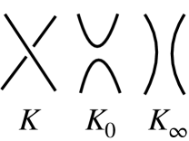
Figure 1. Kauffman triple

The $Y_{K}$ in $\mathcal{S}_{q}[M]$ is invariant under Reidemeister moves II, III and modified Reidemeister move I on $K$ but not under Reidemeister move I.

Figure 2. $Y_{K}$ under Reidemeister move I on $K$.

This is why the $Y_{K}$ is labelled by framed link $K$. We call a link $K=\bigcup_{I=1}^{\sharp(K)}K_{I}$ consisting of $\sharp(K)$ knots an ‘even’ link if

$$\prod_{I=1}^{\sharp(K)}\textrm{sgn}(K_{I})=+1\;,$$

and an ‘odd’ link otherwise. Here $\textrm{sgn}(K_{I})\in\{+1,-1\}$ is defined as

(2) $$\textrm{sgn}(K_{I}):=\begin{cases}+1,\quad\textrm{if $[K_{I}]=1$ as an element of $H_{1}(M,\mathbb{Z}_{2})=\mathbb{Z}_{2}=\{+1,-1\}$\;, }\\ -1,\quad\textrm{otherwise.}\end{cases}$$

For later use, we consider a submodule $\mathcal{S}_{q}^{\rm even}[M]$ whose basis $Y_{K}$ are labelled by even links $K$ on $M$. Note that the Kauffman bracket Skein relation is well-defined in $\mathcal{S}_{q}^{\rm even}$, i.e. all three links in Kauffman triple share the same evenness/oddness and $K\bigsqcup\bigcirc$ is even if $K$ is even.

2.1.1. Skein algebra and trace map

In the special case $q^{1/2}=1$, the Skein module gives rise to the Skein algebra, $V[M]:=\mathcal{S}_{q}[M]|_{q^{1/2}=1}$.

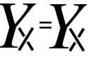
Figure 3. Kauffman bracket Skein relation at $q^{1/2}=1$.

At $q^{1/2}=1$, the Skein relation equates the over-crossing and the under-crossing, as in Figure 3, so that the Skein algebra is a indeed a commutative $\mathbb{C}$-algebra equipped with the multiplication,

(3) $$Y_{K_{1}}Y_{K_{2}}=Y_{K_{2}}Y_{K_{1}}:=Y_{K_{1}\cup K_{2}}\;.$$

The $\mathbb{C}$-algebra is generated by elements in $\pi_{1}(M)$ modulo some relations:

(4) $$\begin{split}V[M]&=\frac{\mathbb{C}[Y_{\gamma}:\gamma\in\pi_{1}(M)]}{\langle Y_{\gamma_{1}}Y_{\gamma_{2}}-Y_{\gamma_{2}}Y_{\gamma_{1}},\;Y_{\gamma_{1}}Y_{\gamma_{2}}+Y_{\gamma_{1}\gamma_{2}}+Y_{\gamma_{1}\gamma_{2}^{-1}}\;,\;Y_{e}+2\rangle}\;,\\ V^{\rm even}[M]&=\{x\in V[M]\;:\;\textrm{$x$ is even}\}\;.\end{split}$$

Here $e\in\pi_{1}(M)$ is the identity element. The above relations imply that $Y_{\gamma}=Y_{\gamma^{-1}}$ and $Y_{\gamma}$ depends only on the conjugacy class of $\gamma$ in $\pi_{1}(M)$. General element $x\in V^{\rm even}[M]$ is given as

$$\sum_{I}C_{I}\prod_{i=1}^{n_{I}}Y_{\gamma^{I}_{i}}\quad\textrm{with $\gamma_{i}^{I}\in\pi_{1}(M),\;C_{I}\in\mathbb{C}$ and $\prod_{i=1}^{n_{I}}\textrm{sgn}[\gamma_{i}^{I}]=1$ for all $I$.}$$

The relations in the denominator come from the relations in the Skein module $\mathcal{S}_{q}[M]$ in eqn.(1) at $q^{1/4}=-1$. We choose $q^{1/4}=-1$ instead of $q^{1/4}=1$ for a later convenience. There is an algebra isomorphism between $\mathcal{S}_{q}[M]$ at $q^{1/4}=1$ and $\mathcal{S}_{q}[M]$ at $q^{1/4}=-1$.

One interesting aspect of the Skein algebra is its relation to the coordinate ring of $SL(2,\mathbb{C})$ character variety $X[M]$, which is defined as

(5) $$\begin{split}&X[M]:=\textrm{Hom}\big{[}\pi_{1}(M)\rightarrow SL(2,\mathbb{C})\big{]}/\sim\\ &\textrm{where }\rho_{1}\sim\rho_{2}\textrm{ if }\textrm{Tr}(\rho_{1}(\gamma))=\textrm{Tr}(\rho_{2}(\gamma))\textrm{ for all $\gamma\in\pi_{1}(M)$}.\end{split}$$

For our purposes, we consider the $\mathbb{Z}_{2}$-quotient of the variety, $X[M]/\mathbb{Z}_{2}$, where the $\mathbb{Z}_{2}$ is the action of $H^{1}(M,\mathbb{Z}_{2})=\textrm{Hom}(\pi_{1}M\rightarrow\mathbb{Z}_{2}=\{\pm 1\})=\{1,\eta\}$:

(6) $$\begin{split}&X[M]/\mathbb{Z}_{2}=\{\rho\in X[M]\}/\sim\;\\ &\textrm{where }\rho_{1}\sim\rho_{2}\textrm{ if }\rho_{1}(\gamma)=\eta(\gamma)\rho_{2}(\gamma)\;\textrm{ for all }\gamma\in\pi_{1}(M)\;.\end{split}$$

One can naturally define an algebra homomorphism $\Phi_{\rm tr}$ called trace map from the Skein algebra $V[M]$ to the coordinate ring $\mathbb{C}[X(M)]$ (or from $V^{\rm even}[M]$ to $\mathbb{C}[X(M)/\mathbb{Z}_{2}]$), the algebra of functions on $X(M)$, as follows

(7) $$\begin{split}&\Phi_{\rm tr}\;:\;V(M)\;\left(\textrm{or }V^{\rm even}(M)\right)\rightarrow\mathbb{C}[X(M)]\;\left(\textrm{or }\mathbb{C}[X(M)/\mathbb{Z}_{2}]\right),\textrm{ where }\\ &[\textrm{$\Phi_{\rm tr}$}(Y_{\gamma})](\rho)=-\textrm{Tr}(\rho(\gamma))\;.\end{split}$$

To see that the map is an algebra homomorphism, one needs to use the following property of $SL(2,\mathbb{C})$ matrices

(8) $$\textrm{Tr}(A)\textrm{Tr}(B)=\textrm{Tr}(AB)+\textrm{Tr}(AB^{-1})\;,\quad\textrm{Tr}(\mathbb{I})=2\;,$$

where $\mathbb{I}$ is the $2\times 2$ identity matrix. The trace map is well-defined as a homomorphism from $V^{\rm even}(M)$ to $\mathbb{C}[X(M)/\mathbb{Z}_{2}]$ since $\prod_{I=1}^{n}\eta(\gamma_{I})=1$ for $\prod_{I=1}^{n}Y_{\gamma_{I}}\in V^{\rm even}(M)$. This section can be summarized by the diagram in Figure 4.

Figure 4. Relations among $\mathcal{S}^{\rm even}_{q}[M]$ (even Kauffman bracket Skein module), $V^{\rm even}[M]$ (even Skein algebra) and $\mathbb{C}[X(M)/\mathbb{Z}_{2}]$ (coordinate ring of character variety). The relations suggest that $\mathcal{S}^{\rm even}_{q}[M]$ can be considered as a quantization of $\mathbb{C}[X(M)/\mathbb{Z}_{2}]$.

For later use, we define the canonical component $X_{0}[M]\subset X[M]$ for a hyperbolic knot complement $M=S^{3}\backslash\mathcal{K}$ as

(9) $$\begin{split}X_{0}[M]&:=\mbox{a connected component of $X[M]$ which contain $\rho_{\rm hyp}$}\;,\\ \rho_{\rm hyp}&:=\mbox{an $SL(2,\mathbb{C})$-representation}\\ &\quad\quad\mbox{corresponding to the complete hyperbolic structure}\;.\end{split}$$

In the same way, one can define $X_{0}(M)/\mathbb{Z}_{2}$.

2.2. Quantum gluing module

Following [Dimofte:2011gm, Gang:2015wya], we define the quantum gluing module $\hat{\mathbb{C}}_{q}[\mathcal{T}]$ associated to an ideal triangulation $\mathcal{T}$ of $M$ as

(10) $$\begin{split}&\hat{\mathbb{C}}_{q}[\mathcal{T}]=\frac{\left(\mathbb{C}[q^{\pm 1/4}][\hat{z}_{i},\hat{z}^{\prime\prime}_{i},\hat{z}^{-1}_{i},\hat{z}_{i}^{\prime\prime-1}])\big{/}\langle\hat{z}_{i}\hat{z}^{\prime\prime}_{j}-q^{-\delta_{ij}}\hat{z}^{\prime\prime}_{j}\hat{z}_{i}\rangle\right)}{\textrm{equivalence relations}\sim}\\ &\textrm{where }\hat{O}\sim e^{\hat{C}_{I}}\cdot\hat{O}\;\textrm{and}\;\hat{O}\sim\hat{O}\cdot(\hat{z}^{-1}_{i}+\hat{z}^{\prime\prime}_{i})\;.\end{split}$$

Here $i$ runs from 1 to $|\mathcal{T}|$, the number of tetrahedra in the ideal triangulation. The precise definition of the exponentiated internal edge operators $e^{\hat{C}_{I}}$ can be found in (LABEL:exponentiated_C) in appendix LABEL:gluing. Before taking the quotient by the equivalence relations, it is a non-commutative algebra. After the quotient, it becomes just a $\mathbb{C}[q^{\pm 1/4}]$-module since the non-commutative multiplication is not compatible with the equivalence relation and thus can not be well-defined in $\hat{\mathbb{C}}_{q}[\mathcal{T}]$.

At $q^{1/2}=1$, $\hat{\mathbb{C}}_{q}[\mathcal{T}]$ becomes the algebra of functions on the gluing equation variety $\chi[\mathcal{T}]$

(11) $$\begin{split}&\hat{\mathbb{C}}_{q}[\mathcal{T}]|_{q^{1/2}=1}\simeq\mathbb{C}[\chi[\mathcal{T}]]\;,\\ &\chi[\mathcal{T}]:=\{z_{i},z_{i}^{\prime\prime}\;:\;z_{i}^{-1}+z_{i}^{\prime\prime}-1=0,\;e^{C_{I}}=1\}_{i=1}^{|\mathcal{T}|}\;.\end{split}$$

For each element $(z_{i},z_{i}^{\prime\prime})\in\chi[\mathcal{T}]$, there is an associated representation [thurston1979geometry]

(12) $$\rho^{\mathcal{T}}_{(z_{,}z^{\prime\prime})}\in\textrm{Hom}[\pi_{1}(S^{3}\backslash\mathcal{K})\rightarrow PSL(2,\mathbb{C})]$$

We choose an ideal triangulation $\mathcal{T}$ which is a $\rho_{\rm hyp}$-regular:

(13) $$\textrm{$\mathcal{T}$ is called $\rho_{\rm hyp}$-regular if $\exists(z,z^{\prime\prime})_{\rm hyp}\in\chi[\mathcal{T}]$ such that $\rho^{\mathcal{T}}_{(z,z^{\prime\prime})_{\rm hyp}}=\rho_{\rm hyp}$}\;.$$

$\rho_{\rm hyp}$ is an $SL(2,\mathbb{C})$-representation in (9) but also can be regarded as an $PSL(2,\mathbb{C})=SL(2,\mathbb{C})/\mathbb{Z}_{2}$-representation. Let us denote by $\chi_{0}[\mathcal{T}]$ the connected component of $\chi[\mathcal{T}]$ which contains $(z,z^{\prime\prime})_{\rm hyp}$. In general, the gluing equation variety $\chi[\mathcal{T}]$ depends on the choice of $\rho_{\rm hyp}$-regular triangulation $\mathcal{T}$ while the $\chi_{0}[\mathcal{T}]$ does not [tillmann2012degenerations]. The component can be identified with

(14) $$\chi_{0}[\mathcal{T}]\simeq X_{0}(M)/\mathbb{Z}_{2}\;.$$

Another nice reason for restricting to the component $\chi_{0}[\mathcal{T}]$ is that any $PSL(2,\mathbb{C})=SL(2,\mathbb{C})/\mathbb{Z}_{2}$ representation $\rho^{\mathcal{T}}_{(z,z^{\prime\prime})}$ with $(z,z^{\prime\prime})\in\chi_{0}[\mathcal{T}]$ can be lifted to a $SL(2,\mathbb{C})$ representation. Thus, one can define the classical trace map $\Phi_{\rm tr}:V^{\rm even}[M]\rightarrow\mathbb{C}[\chi_{0}[\mathcal{T}]]$ as follows

(15) $$[\Phi(Y_{\gamma})](z,z^{\prime\prime})=-\textrm{Tr}(\rho_{(z,z^{\prime\prime})}^{\mathcal{T}}(\gamma))\;.$$

The trace map is identical to the map in (7) under the identification $\chi_{0}(\mathcal{T})\simeq X_{0}[M]/\mathbb{Z}_{2}$. The lifting from $PSL(2,\mathbb{C})$-representation to $SL(2,\mathbb{C})$-representation is not unique and the two different upliftings, $\rho$ and $\tilde{\rho}$, are related by the action of $H^{1}(S^{3}\backslash\mathcal{K},\mathbb{Z}_{2})=\textrm{Hom}[\pi_{1}(S^{3}\backslash\mathcal{K})\rightarrow\mathbb{Z}_{2}]=\{1,\eta\}$, i.e.

(16) $$\tilde{\rho}(\gamma)=\eta(\gamma)\rho(\gamma)\;,\quad$$

For even $Y_{\gamma}\in V^{\rm even}[M]$, the trace map is well-defined, i.e. independent of the choice of liftings, since $\eta(\gamma)=1$.

2.3. Quantum trace map and Length conjecture

The quantum trace map for 2D surfaces with $SL(2)$ was introduced in [bonahon2010quantum], and was generalized to groups of higher rank in [Gabella:2016zxu]. Here we introduce a 3D version of the quantum trace map.

Figure 5. Quantum trace map.

Conjecture 2.1 (main conjecture).

There exists a unique injective module homomorphism $\textrm{tr}^{\mathcal{T}}_{q}:\mathcal{S}^{\rm even}_{q}[M]\rightarrow\hat{\mathbb{C}}_{q}[\mathcal{T}]$ which satisfies the following properties:

I. At $q^{1/4}=-1$, the quantum trace map is identical to the trace map $\Phi_{\rm tr}$

(17) $$(\textrm{tr}_{q}^{\mathcal{T}})\big{|}_{q^{1/4}=-1}=\Phi_{\rm tr}\quad\textrm{as a map $V^{\rm even}(M)\rightarrow\mathbb{C}[X_{0}(M)/\mathbb{Z}_{2}]$}\;.$$

The relation between $\textrm{tr}^{\mathcal{T}}_{q}$ and $\Phi_{\textrm{tr}}$ is summarized in Figure 5.

II. (All-order length conjecture) For an even link $K=\bigcup_{I=1}^{\sharp(K)}K_{I}\subset M=S^{3}\backslash\mathcal{K}$,

(18) $$\begin{split}&\frac{J_{n,\tilde{n}_{I}=2}(\mathcal{K}\cup K;q)}{J_{n}(\mathcal{K};q)}\bigg{|}_{q^{1/4}=-\exp(\frac{\pi i}{2k})}\xrightarrow{\quad n=k;\;k\rightarrow\infty\quad}\sum_{s=0}^{\infty}\mathcal{Z}^{\rm(hyp)}_{s}(\hat{O}_{K};M)\left(\frac{2\pi i}{k}\right)^{s}\;.\\ &\textrm{or equivalently},\\ &\log\frac{J_{n,\tilde{n}_{I}=2}(\mathcal{K}\cup K;q)}{J_{n}(\mathcal{K};q)}\bigg{|}_{q^{1/4}=-\exp(\frac{\pi i}{2k})}\xrightarrow{\quad n=k;\;k\rightarrow\infty\quad}\sum_{s=0}^{\infty}\mathcal{W}^{\rm(hyp)}_{s}(\hat{O}_{K};M)\left(\frac{2\pi i}{k}\right)^{s}\;.\end{split}$$

Here $J$ denotes a variation of the colored Jones polynomial for framed links. While the conventional colored Jones polynomial is an invariant of oriented links, our $J$ is an invariant of unoriented framed links. See Appendix LABEL:Appendix_:_Jones_polynomial for the definition. In the above, $I=1,\ldots,\sharp(K)$ and $\tilde{n}_{I}$ denotes the ‘color’ of the $I$-th component.

The perturbative invariant $\mathcal{W}^{\rm(hyp)}_{s}(\hat{O}_{K};M)$ is determined by the quantum trace operator

(19) $$\hat{O}_{K}:=\textrm{tr}_{q}^{\mathcal{T}}(Y_{K})\;.$$

More generally, for an element $Y=\sum_{a}C_{a}Y_{K_{a}}\in\mathcal{S}_{q}^{\rm even}[M]$,

(20) $$\hat{O}_{Y}:=\textrm{tr}^{\mathcal{T}}_{q}(Y)=\sum_{a}C_{a}\hat{O}_{K_{a}}\;.$$

The operator $\hat{O}_{K}$ is a $\hat{\mathbb{C}}_{q}[\mathcal{T}]$-valued invariant of unoriented framed links.

By incorporating the $\hat{O}$ with the state-integral model [Dimofte:2011gm], the perturbative invariants $\{\mathcal{W}^{\rm(hyp)}_{s}(\hat{O}_{K};M),\mathcal{Z}^{\rm(hyp)}_{s}(\hat{O}_{K};M)\}_{s=0}^{\infty}$ can be obtained from the perturbative expansion of the state-integral model. The explicit form of the state-integral model and its perturbative expansion using Feynman diagram will be given in section 3.

Two perturbative expansions are related to each other by exponential or logarithm, i.e.

(21) $$\exp\left(\sum_{s=0}^{\infty}\mathcal{W}^{\rm(hyp)}_{s}\hbar^{s}\right)=\sum_{s=0}^{\infty}\mathcal{Z}^{\rm(hyp)}_{s}\hbar^{s}\textrm{ as a formal power series in $\hbar$}.$$

The leading “classical” coefficient $\mathcal{Z}^{\rm hyp}_{s=0}(\hat{O}_{K};M)$ is simply given by

(22) $$\mathcal{Z}^{\rm(hyp)}_{s=0}(\hat{O};M):=\left(\hat{O}|_{q^{1/4}\rightarrow-1}\right)\bigg{|}_{(z_{i},z^{\prime\prime}_{i})=(z^{\prime}_{i},z^{\prime\prime}_{i})_{\rm hyp}}\;.$$

Here $\hat{O}|_{q^{1/4}\rightarrow-1}$ is regarded as an element in $\mathbb{C}[\chi_{0}(\mathcal{T})]$. The classical value is

(23) $$\begin{split}&\mathcal{Z}^{\rm hyp}_{s=0}(\hat{O}_{K};M)=\textrm{Tr}\left([\Phi_{\rm tr}(Y_{\gamma_{K}})](\rho_{\rm hyp})\right)\;,\\ &\textrm{or equivalently, }\mathcal{W}^{\rm(hyp)}_{s=0}(\hat{O}_{K};M)=\log\left([\Phi_{\rm tr}(Y_{\gamma_{K}})](\rho_{\rm hyp})\right)\,.\end{split}$$

Here $Y_{\gamma_{K}}=\prod_{I=1}^{n}Y_{\gamma_{I}}$ is an element of the Skein algebra obtained from $Y_{K}$ at $q^{-1/4}=-1$ and $\rho_{\rm hyp}\in\textrm{Hom}[\pi_{1}(M)\rightarrow SL(2,\mathbb{C})]$ is an $SL(2,\mathbb{C})$ flat connection corresponding to the complete hyperbolic structure on $M$. The classical part is related to the complex length of the geodesic (hence the name “length conjecture”) by

(24) $$[\Phi_{\rm tr}(Y_{\gamma_{K}})](\rho_{\rm hyp}):=\prod_{I=1}^{\sharp(K)}\left(-\textrm{Tr}(\rho_{\rm hyp}(\gamma_{I}))\right)=\prod_{I=1}^{\sharp(K)}(-e^{\frac{1}{2}\ell_{\mathbb{C}}(\gamma_{I})}-e^{-\frac{1}{2}\ell_{\mathbb{C}}(\gamma_{I})})\;.$$

$\ell_{\mathbb{C}}(\gamma_{I})$ denotes the complexified length of a geodesic in the same homotopy class as $\gamma_{I}$ of $K_{I}$

To prove the length conjecture in (18) and (23), we only need to prove them for basis $\{Y_{K_{a}}\}$ of $\mathcal{S}^{\rm even}_{q}[M]$. It is obvious for (18) since for $Y_{K}=\sum_{a}C_{a}(q^{1/4})Y_{K_{a}}$,

(25) $$J_{n,\tilde{n}_{I}=2}(\mathcal{K}\cup K;q)=\sum_{a}C_{a}(q^{1/4})J_{n,\tilde{n}_{I}=2}(\mathcal{K}\cup K_{a};q)\,,$$

and the perturbative invariants $\mathcal{Z}_{s}^{\rm(hyp)}(\hat{O}_{Y_{K}})$ satisfy

(26) $$\sum_{s=0}^{\infty}\mathcal{Z}^{\rm(hyp)}_{s}(\hat{O}_{K};M)\hbar^{s}=\sum_{a}C_{a}(q^{1/4}=-e^{\frac{\hbar}{4}})\left(\sum_{s}\mathcal{Z}^{\rm(hyp)}_{s}(\hat{O}_{K_{a}};M)\hbar^{s}\right)\;.$$

The relation in (23) is valid for arbitrary $\hat{O}_{K}$ if it holds for every basis since

(27) $$\begin{split}&\Phi_{\rm tr}(Y_{\gamma_{K}})(\rho)=\sum_{a}C_{a}(q^{1/4}=-1)\Phi_{\rm tr}(Y_{\gamma_{K}})(\rho)\;,\\ &\textrm{for arbitrary $\rho\in\textrm{Hom}\left[\pi_{1}M\rightarrow SL(2,\mathbb{C})\right]$}\;,\end{split}$$

which follows from the fact that the quantum trace map $\textrm{tr}_{q}^{\mathcal{T}}$ is a module homomorphism and it becomes the classical trace map $\Phi_{\rm tr}$ in (7) at $q^{1/4}=-1$.

III. For an even link $K$ and a meridian knot $\bigcirc_{\rm m}$, a knot linking the heavy knot $\mathcal{K}$,

(28) $$\begin{split}\hat{O}_{K\sqcup\bigcirc^{2}_{\rm m}}=\hat{O}_{\bigcirc^{2}_{\rm m}}\cdot\hat{O}_{K}\;,\quad\textrm{where}\quad\hat{O}_{\bigcirc^{2}_{\rm m}}:=2+e^{\hat{\mathfrak{M}}}+e^{-\hat{\mathfrak{M}}}\;.\end{split}$$

See (LABEL:exponentiated_M) for the definition of $e^{\pm\hat{\mathfrak{M}}}$ and Figure LABEL:fig:_Reidemeister_move_1p for the knot $\bigcirc_{\rm m}$. The operator $\hat{O}_{\bigcirc^{2}_{\rm m}}$ always commutes with $e^{\hat{C}_{I}}$ and thus the left multiplication is well-defined in $\hat{\mathbb{C}}_{q}[\mathcal{T}]$. In section 3, we will see that

(29) $$\sum_{s=0}^{\infty}\mathcal{Z}^{\rm(hyp)}_{s}(\hat{O}_{K\sqcup\bigcirc^{2}_{\rm m}})\hbar^{s}=4\sum_{s=0}^{\infty}\mathcal{Z}^{\rm(hyp)}_{s}(\hat{O}_{K})\hbar^{s}$$

for an arbitrary knot $K$ in $M=S^{3}\backslash\mathcal{K}$. It is compatible with the all-order length conjecture (18) since

(30) $$\begin{split}&J_{n,\tilde{n}_{I}=2}(\mathcal{K}\cup(K\sqcup\bigcirc^{2}_{\rm m}))=(q^{n/2}+q^{-n/2})^{2}\times J_{n,\tilde{n}_{I}=2}(\mathcal{K}\cup K)\;,\\ &\textrm{and }(q^{n/2}+q^{-n/2})^{2}|_{q=\exp(2\pi i/k),n=k}=4\;.\end{split}$$

Here we use the property of our Jones polynomial depicted in Figure LABEL:fig:_Reidemeister_move_1p .

3. Perturbative knot invariants

We recall and extend state-integral models from [Dimofte:2011gm, Dimofte:2012qj, Gang:2015wya] to define the perturbative knot invariants $\{\mathcal{Z}_{s}^{\rm(hyp)}(\hat{O}_{K};M)\}_{s=0}^{\infty}$.

3.1. State-integral model with quantum trace map

The state-integral model is based on an ideal triangulation $\mathcal{T}$ of $M=S^{3}\backslash\mathcal{K}$ and can be written as in the following form using Dirac brackets ($k:=|\mathcal{T}|$)

(31) $$\begin{split}&Z_{\hbar}[M+\hat{O};X_{\bf m}]\\ &=\langle X_{\bf m},C_{1},\ldots,C_{k-1};\Pi_{M,C}|\hat{O}(q^{\frac{1}{4}}=-e^{\frac{\hbar}{4}})|\Delta^{\otimes k}\rangle\big{|}_{C_{1}=\ldots=C_{k-1}=0}\;,\\ &=\int\prod_{i=1}^{k}\frac{dZ_{i}}{\sqrt{2\pi\hbar}}\langle X_{\bf m},C_{1},\ldots,C_{k-1};\Pi_{M,C}|Z_{1},\ldots,Z_{k};\Pi_{Z}\rangle\langle Z_{1},\ldots,Z_{k};\Pi_{Z}|\hat{O}|\Delta^{\otimes k}\rangle\;.\end{split}$$

The state-integral is a function on a meridian variable $X_{\bf m}$. Here $|X_{1},\ldots,X_{k};\Pi_{X}\rangle$ denotes the position basis of $\left(\mathcal{H}(\partial\Delta)\right)^{\otimes k}$, the Hilbert-space associated with the $k$-tetrahedra [Dimofte:2011gm], with respect to a polarization choice $\Pi_{X}=(X_{1},\ldots,X_{k},P_{1},\ldots,P_{k})^{T}$:

(32) $$\begin{split}&\langle X_{1},\ldots,X_{k};\Pi_{X}|e^{\hat{X}_{i}}|\psi\rangle=e^{X_{i}}\langle X_{1},\ldots,X_{k};\Pi_{X}|\psi\rangle\;\textrm{ and }\\ &\langle X_{1},\ldots,X_{k};\Pi_{X}|e^{\hat{P}_{i}}|\psi\rangle=\langle X_{1},\ldots,X_{k};\Pi_{X}|\psi\rangle|_{X_{i}\rightarrow X_{i}+\hbar},\;\forall|\psi\rangle\in\left(\mathcal{H}(\partial\Delta)\right)^{\otimes k}\;.\end{split}$$

Here two polarizations $\Pi_{M,C}$ and $\Pi_{Z}$ are

(33) $$\Pi_{M,C}=\begin{pmatrix}\mathfrak{M}\\ C_{1}\\ \ldots\\ C_{k-1}\\ \frac{1}{2}\mathfrak{L}\\ \Gamma_{1}\\ \ldots\\ \Gamma_{k-1}\end{pmatrix}\;,\quad\Pi_{Z}=\begin{pmatrix}Z_{1}\\ Z_{2}\\ \ldots\\ Z_{k}\\ Z^{\prime\prime}_{1}\\ Z^{\prime\prime}_{2}\\ \ldots\\ Z_{k}^{\prime\prime}\end{pmatrix}$$

and they are related to each other by a linear canonical transformation

(34) $$\Pi_{M,C}=g\cdot\Pi_{Z}-(i\pi+\frac{\hbar}{2})\begin{pmatrix}\vec{\nu}\\ \vec{\nu}_{p}\end{pmatrix}\;,\;\;\textrm{ where }g\in Sp(2k,\mathbb{Z})\textrm{ and }\vec{\nu},\vec{\nu}_{p}\in\mathbb{Z}^{k}\;.$$

$\Gamma$’s are chosen such that the linear transformation becomes a canonical transformation. The choice is not unique but the final state-integral does not depend on it. The two position bases are related to each other by following unitary transformation

(35) $$\begin{split}&\langle X_{\bf m},C_{1},\ldots,C_{k-1};\Pi_{M,C}|Z_{1},\ldots,Z_{k};\Pi_{Z}\rangle\\ &\hskip 85.35826pt=\frac{1}{\sqrt{\det B}}\exp\left(\frac{1}{2\hbar}Q(\vec{X},\vec{Z})\right)\bigg{|}_{\vec{X}=(X_{\mathbf{m}},C_{1},\cdots,C_{k-1})}^{\vec{Z}=(Z_{1},\ldots,Z_{k})}\\ &\textrm{with}\\ &Q(\vec{X},\vec{Z})=\vec{Z}B^{-1}A\vec{Z}+\vec{X}DB^{-1}\vec{X}+(2\pi i+\hbar)\vec{f}B^{-1}\vec{X}+(i\pi+\frac{\hbar}{2})^{2}\vec{f}B^{-1}\vec{\nu}\\ &\qquad\qquad\;\;-\vec{Z}B^{-1}((2i\pi+\hbar)\vec{\nu}+2\vec{X})\;.\end{split}$$

Here $A,B,C$ and $D$ are the four $(k\times k)$ block matrices of $g$:

(36) $$g=\begin{pmatrix}A&B\\ C&D\end{pmatrix}\;.$$

The vectors $(\vec{f},\vec{f}^{\prime\prime})=(f_{i},f_{i}^{\prime\prime})_{i=1}^{k}$ are known as combinatorial flattening, and chosen to satisfy the following relation

(37) $$\begin{pmatrix}A&B\\ C&D\end{pmatrix}\cdot\begin{pmatrix}\vec{f}\\ \vec{f}^{\prime\prime}\end{pmatrix}=\begin{pmatrix}\vec{\nu}\\ \vec{\nu}_{p}\end{pmatrix}\;.$$

$|\Delta^{\otimes k}\rangle\in\left(\mathcal{H}(\partial\Delta)\right)^{\otimes k}$ is the wave-function for $k$-tetrahedra satisfying the following difference equations

(38) $$(e^{\hat{Z}^{\prime\prime}_{i}}+e^{-\hat{Z}_{i}}-1)|\Delta^{\otimes k}\rangle=0\;,\quad i=1,\ldots k.$$

In the polarization $\Pi_{Z}$, the wave-function is given by a product of quantum dilogarithms (see Appendix LABEL:App_:_QDL for our convention for the quantum dilogarithm)

(39) $$\langle Z_{1},\ldots,Z_{k};\Pi_{Z}|\Delta^{\otimes k}\rangle=\prod_{i=1}^{k}\psi_{\hbar}(Z_{i})\;.$$

Gathering all the expressions above, one has

(40) $$\begin{split}&Z_{\hbar}[M+\hat{O};X_{\bf m}]\\ &=\frac{1}{\sqrt{\det B}}\sum_{\alpha}C_{\alpha}(q^{\frac{1}{4}})\big{|}_{q^{\frac{1}{4}}=-e^{\frac{\hbar}{4}}}\int\prod_{i=1}^{k}\frac{dZ_{i}}{\sqrt{2\pi\hbar}}\exp\left(\frac{1}{2\hbar}Q(\vec{X},\vec{Z})\right)\bigg{|}_{\vec{X}=(X_{\mathbf{m}},\cdots,C_{k-1})}^{\vec{Z}=(Z_{1},\ldots,Z_{k})}\\ &\qquad\qquad\qquad\qquad\qquad\qquad\qquad\times\langle Z_{1},\ldots,Z_{k};\Pi_{Z}|\prod_{i}\hat{z}_{i}^{a_{i}^{(\alpha)}}(\hat{z}^{\prime\prime}_{i})^{b_{i}^{(\alpha)}}|\Delta^{\otimes k}\rangle\;,\\ &=\frac{1}{\sqrt{\det B}}\sum_{\alpha}C_{\alpha}(q^{\frac{1}{4}})\big{|}_{q^{\frac{1}{4}}=-e^{\frac{\hbar}{4}}}\int\prod_{i=1}^{k}\frac{dZ_{i}}{\sqrt{2\pi\hbar}}\exp\left(\frac{1}{2\hbar}Q(\vec{X},\vec{Z})\right)\bigg{|}_{\vec{X}=(X_{\mathbf{m}},\cdots,C_{k-1})}^{\vec{Z}=(Z_{1},\ldots,Z_{k})}\\ &\qquad\qquad\qquad\qquad\qquad\qquad\qquad\times\prod_{i=1}^{k}\psi_{\hbar}(Z_{i}+b_{i}^{(\alpha)}\hbar)\exp\left(a_{i}^{(\alpha)}Z_{i}\right)\;,\end{split}$$

when $\hat{O}=\sum_{\alpha}C_{\alpha}(q^{\frac{1}{4}})\prod_{i}\hat{z}_{i}^{a^{(\alpha)}_{i}}(\hat{z}^{\prime\prime}_{i})^{b^{(\alpha)}_{i}}\in\hat{\mathbb{C}}_{q}[\mathcal{T}]$. From the expression in (31), it is not difficult to see that the $Z_{\hbar}[M+\hat{O};X_{\bf m}]$ with $\hat{O}\in\hat{\mathbb{C}}_{q}[\mathcal{T}]$ is well-defined (recall the definition of $\hat{\mathbb{C}}_{q}[\mathcal{T}]$ in (10)), i.e.

(41) $$Z_{\hbar}[M+\hat{O}]=Z_{\hbar}[M+e^{\hat{C_{I}}}\cdot\hat{O}]=Z_{\hbar}[M+\hat{O}\cdot(\hat{z}_{i}^{-1}+\hat{z}^{\prime\prime}_{i})]$$

It is also straightforward to see that

(42) $$Z_{\hbar}[M+F(e^{\hat{\mathfrak{M}}})\cdot\hat{O}]=F(e^{X_{\bf m}})Z_{\hbar}[M+\hat{O}]\;,$$

for arbitrary Laurent polynomial $F(z)$ and $\hat{O}\in\hat{\mathbb{C}}_{q}[\mathcal{T}]$.

3.2. Perturbative invariants

We are ready to define and explain the perturbative invariants $\{\mathcal{Z}^{(\rm hyp)}_{s}(\hat{O};M)\}_{s=0}^{\infty}$. By expanding the state-integral in the limit $\hbar\rightarrow 0$ around the saddle point $\vec{Z}^{(\rm hyp)}$ associated to complete hyperbolic structure of $M$, one have

(43) $$Z_{\hbar}[M+\hat{O};X_{\bf m}=0]\xrightarrow{\quad\hbar\rightarrow 0\quad}\exp\left(\sum_{n=0}^{\infty}S_{n}^{(\rm hyp)}(\hat{O};M)\hbar^{n-1}\right)\;.$$

In the expansion, one can use the asymptotic expansion of the quantum dilogarithm function in (LABEL:eq:psi_expansoin). Then, we define the perturbative invariants $\{\mathcal{Z}^{(\rm hyp)}_{s},\mathcal{W}^{(\rm hyp)}_{s}\}_{s=0}^{\infty}$ as

(44) $$\begin{split}\frac{\exp\left(\sum_{n=0}^{\infty}S_{n}^{(\rm hyp)}(\hat{O};M)\hbar^{n-1}\right)}{\exp\left(\sum_{n=0}^{\infty}S_{n}^{(\rm hyp)}(M)\hbar^{n-1}\right)}&=\sum_{s=0}^{\infty}\mathcal{Z}_{s}^{(\rm hyp)}(\hat{O};M)\hbar^{s}\\ &=\exp\left(\sum_{s=0}^{\infty}\mathcal{W}_{s}^{(\rm hyp)}(\hat{O};M)\hbar^{s}\right)\;.\end{split}$$

Here $S_{n}^{\rm(hyp)}(M):=S_{n}^{\rm(hyp)}(\hat{O}_{K=\emptyset};M)$ is the perturbative invariant of state-integral model without any insertion of loop operator. From the definition, one can see that the relation in (29) simply follows from (42) with $F(x)=2+x+\frac{1}{x}$ and $X_{\bf m}=0$. In the classical limit $\hbar\rightarrow 0$, saddle points $\{\vec{Z}=\vec{Z}^{(\alpha)}\}$ of the state-integral at $X_{\bf m}=0$ satsify following equations

(45) $$\prod_{j=1}^{k}z_{j}^{A_{ij}}(1-z^{-1}_{j})^{B_{ij}}\big{|}_{z_{i}=\exp(Z_{i}^{(\alpha)})}=(-1)^{\nu_{i}}\;.$$

For $\rho_{\rm hyp}$-regular ideal triangulation $\mathcal{T}$, the saddle point $\vec{Z}^{(\rm hyp)}$ is uniquely characterized by following conditions ($z^{(\rm hyp)}_{i}:=\exp(Z^{(\rm hyp)}_{i})$)

(46) $$\textrm{Im}[z^{(\rm hyp)}_{i}]<0\quad\textrm{for all }i=1,\ldots,k\;.$$